Embed Size (px)
Citation preview
INTERNATIONAL ECONOMIC REVIEWVol. 50, No. 4, November 2009
FORMAL HOME HEALTH CARE, INFORMAL CARE, AND FAMILYDECISION MAKING∗
BY DAVID BYRNE, MICHELLE S. GOEREE, BRIDGET HIEDEMANN, AND STEVEN STERN1
Federal Reserve Board, U.S.A.; University of Zurich, Switzerland, University of SouthernCalifornia, U.S.A.; University of Seattle, U.S.A.; University of Virginia, U.S.A.
We use the 1993 wave of the Assets and Health Dynamics Among the Oldest Old (AHEAD) data set to estimate agame-theoretic model of families’ decisions concerning the provision of informal and formal care for elderly individuals.The outcome is the Nash equilibrium where each family member jointly determines her consumption, transfers for formalcare, and allocation of time to informal care, market work, and leisure. We use the estimates to decompose the effectsof adult children’s opportunity costs, quality of care, and caregiving burden on their propensities to provide informalcare. We also simulate the effects of a broad range of policies of current interest.
1. INTRODUCTION
Increased life expectancies in recent decades have contributed to the aging of the popula-tion. Between 1980 and 2000, for example, the elderly population, defined as individuals aged65 years and older, increased by 37%. Demographers predict that the elderly population willreach 71 million, or 20% of the total population, by 2030. As of 2004, the oldest old population,those 85 years and older, was growing three times faster than the general population (U.S. CensusBureau, 2004). Although disability rates among the elderly decreased between 1982 and 1999(Manton and Gu, 2001), the number of disabled elderly individuals has remained approximatelyconstant at 5.5 million because of population aging and the increased level of disability amongthose receiving long-term care (Spector et al., 2001).
Population aging has coincided with dramatic changes in care arrangements for the elderly.Informal care (i.e., unpaid care) has become less common, whereas formal home health care(i.e., paid care) and institutional care have become more widespread (Boersch-Supan et al.,1988; Wolf and Soldo, 1988). For example, about 25% of the oldest old lived in institutionsin 1990 compared to 7% in 1940 (Kotlikoff and Morris, 1990). Although formal home healthcare was relatively uncommon until recent decades, 1.4 million individuals received this form ofcare in 2000. Between 1989 and 1999, the number of informal caregivers rose only 6%, whereasthe elderly population increased 13% (Mack and Thompson, 2004). Despite the trends towardinstitutional and formal home health care, adult children and spouses continue to enable elderlyindividuals to remain in the community; in fact, most elderly who remain in the community doso with the assistance of familial and social networks (e.g., Matthews and Rosner, 1988).
Elder care arrangements have profound economic, social, and psychological implications. Thehigh cost of institutional care often exhausts the resources of nursing home residents. As a con-sequence, many elderly individuals and their families rely on Medicaid to cover their long-termcare expenses. In addition to the financial burden borne by families and by society, institutional
∗ Manuscript received March 2004; revised June 2008.1 We would like to thank Shelly Lundberg, Robert Moffitt, Liliana Pezzin, Stephanie Schmidt, Frank Sloan, Ken
Wolpin, and workshop participants at Duke, Maryland, Penn, Queens, RAND, Seattle, Toronto, University CollegeLondon, Virginia, and Western Ontario for helpful comments. All remaining errors are ours. The views expressed arenot necessarily the views of the Federal Reserve System. Please address correspondence to: Steven Stern, Departmentof Economics, University of Virginia, Charlottesville, VA 22901. Phone: 434 924 6754, Fax: 434 982 2904. E-mail:[email protected].
1205C© (2009) by the Economics Department of the University of Pennsylvania and the Osaka University Institute of Socialand Economic Research Association
1206 BYRNE ET AL.
care typically involves social and psychological costs for elderly individuals (Macken, 1986).Although less expensive than institutional care, home health care consumes an increasing shareof health care expenditures (National Center for Health Statistics, 1996; U.S. Department ofHealth and Human Services, 2000). Care provided by family members typically does not im-pose explicit financial costs, but the opportunity costs in terms of forgone earnings or nonmarkettime can be substantial. Also, the provision of informal care can be psychologically burdensomefor caregivers.
In light of population aging, the changing patterns of elder care, and the profound implicationsof care arrangements for the recipients of care, their families, and society, the development ofappropriate public policies requires an understanding of families’ elder care decisions. We focuson the provision of informal and formal home health care for the noninstitutionalized elderly.Specifically, we construct a game-theoretic model of family decision making where each familymember makes decisions concerning the provision of informal and formal care as part of abroader utility maximization problem. We use the 1993 wave of the Assets and Health DynamicsAmong the Oldest Old (AHEAD) data to estimate our game-theoretic model. Results of thismodel provide insight concerning the role of demographic characteristics and public policiesin families’ care decisions and the welfare of family members. We use the results to simulatethe effects of subsidizing informal and formal care and relaxing the requirements for Medicaidqualification. The model is an early step in developing and estimating structural models of familydecision making and long-term care decisions.
2. LITERATURE REVIEW
Although predominantly empirical, the literature on caregiving for the elderly offers severaltheoretical models. These models vary along several dimensions: whether family members sharecommon preferences, which family members participate in the decision-making process, whichtypes of care arrangements are considered, and whether other decisions are determined jointlywith parental care decisions.
Some papers in the elder care literature assume that a single household utility function isappropriate in the context of elderly parents and their adult children. For example, Hoerger,Picone, and Sloan’s (1996) (HPS) model involves a family utility function and budget constraint.2
Some of the other models,3 including the one presented in this study, are game-theoretic andthus involve separate utility functions for each family member.
Several of the existing theoretical models involve only one child in the decision-making pro-cess.4 This assumption considerably simplifies modeling and estimation but obscures the dy-namics within the younger generation. In practice, more than one adult child in a family mayparticipate in the family’s care decision, and adult siblings may disagree regarding the best sourceof care for an elderly parent. The potential disagreement among adult siblings and between adultchildren and elderly parents motivates the development of a game-theoretic framework wherethe players include the parent, spouse, and all of her5 children. Moreover, the burden associ-ated with caregiving may generate strategic interaction among family members. For example,an adult child’s provision of informal care for her father may depend on the amount of informalcare provided by her siblings and by her mother. Although altruistic toward her father, the adultchild may have incentive to free ride on her siblings’ or her mother’s informal care. Thus, her
2 In Kotlikoff and Morris (1990), parent and child solve separate maximization problems if they live separately butmaximize a weighted average of their individual utility functions subject to their pooled budget constraint if they livetogether.
3 See Pezzin and Schone (1997, 1999), Sloan et al. (1997), Hiedemann and Stern (1999), Checkovich and Stern (2002),and Engers and Stern (2002).
4 Pezzin and Schone (1997, 1999) and Sloan et al. (1997) present models that apply to families of any size, but onlyone child plays a role in the family’s care decision.
5 Throughout the article, we use female pronouns as the generic pronouns. This does not mean that only mothersneed care or that only daughters provide care.
FAMILIES’ ELDER CARE DECISIONS 1207
provision of informal care may depend negatively on the amount of care provided by otherfamily members. Alternatively, in the spirit of Bernheim et al. (1985), a bequest motive couldinduce siblings to compete with one another for a greater share of the inheritance. Thus, anadult child’s provision of informal care could depend positively on the amount of care providedby a sibling. Similarly, siblings may have incentive to free ride on one another with respect tofinancial transfers for formal home health care. The possibility of such strategic play suggeststhat a noncooperative model may be appropriate in the context of families’ caregiving decisionsfor the elderly.
As part of an effort to develop more realistic models of family decision making, Hiedemannand Stern (1999) (HS), Checkovich and Stern (2002) (CS), Engers and Stern (2002) (ES), and thecurrent study present game-theoretic models that accommodate a variable number of childrenand the possibility that all children play a role in care decisions. Whereas HS and ES develop andestimate stylized games that cannot be identified from one another given the available data (ES),the current article considers a much more intuitive game and equilibrium. Here, each agent max-imizes a relatively standard utility function in the context of the Nash equilibrium. The currentarticle also differs from previous work with respect to the scope of care decisions modeled. HSand ES model the decision to provide informal care, whereas CS model the quantity of informalcare provided. Here, we consider both of these choices—whether and how much informal careto provide—in a broader utility maximization framework. In the current model, family membersmake informal care decisions jointly with decisions concerning financial contributions for homehealth care, consumption, market work, and leisure.
Given the variety of care arrangements and the connection between care arrangementsand living arrangements, one model cannot capture all possible aspects of a family’s parentalcare and living arrangements. Whereas Pezzin and Schone (1997), Sloan et al. (1997) (SPH),HS, CS, and ES focus on care arrangements, HPS and Pezzin and Schone (1999)(PS) modelboth care and living arrangements.6 We present a model in which each family member decideshow much informal and formal home health care to provide for elderly parents, taking livingarrangements as given. This study is most closely related to those of SPH, PS, and CS. PS jointlymodel living arrangements with the provision of care by the child (in this case, a daughter). SPHpresent a model in which the choice variables are not the type of care or living arrangement buthours of formal care and informal care provided by the child. CS model each child’s provision ofinformal care. Finally, the provision of care by adult children may be determined simultaneouslywith labor force behavior. As in our study, Ettner (1996) and Pezzin and Schone (1997, 1999)model labor force participation of adult children jointly with care and/or living arrangements.7
The econometric models in the elder care literature are as varied as the theoretical models.Most papers present results based on nonstructural models.8 But several recent papers presentresults based on structural models.9 With the exception of CS and this article, existing studiesfocus on the role of a single child in each family as the primary caregiver and ignore the possibilityof other children serving as sources of assistance.10 However, data from the 1984 National Long-term Care Survey indicate that shared caregiving is an important phenomenon, especially in
6 In a related literature, Kotlikoff and Morris (1990) focus on living arrangements including residence in a nursinghome.
7 The long-term care literature addresses other factors that may play a role in the family’s care decisions. For instance,inter- or intragenerational transfers may be made as part of a family’s long-term care decision. This possibility may becaptured by assuming that the family pools its income (e.g., HPS) or by explicitly modeling side payments among familymembers. PS model intergenerational cash transfers jointly with caregiving, intergenerational household formation, andlabor force behavior. In one of the models in ES, family members choose the long-term care alternative that maximizestheir joint payoff and make any necessary side payments among themselves.
8 See Wolf and Soldo (1988), Lee et al. (1990), Cutler and Sheiner (1993), Ettner (1996), HPS, Boaz and Hu (1997),Diwan et al. (1997), Norgard and Rodgers (1997), SPH, White-Means (1997), and Couch et al. (1999).
9 See Pezzin and Schone (1997, 1999), HS, CS, and ES.10 See Frankfather et al. (1981), Johnson and Catalano (1981), Cantor (1983), Johnson (1983), Stoller and Earl (1983),
Horowitz (1985), Barber (1989), Miller and Montgomery (1990), Stern (1994, 1995, 1996), Pezzin and Schone (1997,1999), HS, and ES.
1208 BYRNE ET AL.
large families. CS show, for example, that over 4% of families with two children, almost 10%of families with three children, and about 16% of families with four children contain multiplecaregivers. Among families where at least one child provides care, the probability that childrenshare caregiving is almost 13% in families with two children, over 25% in families with threechildren, and almost 35% in families with four children. Even if each family relies on a singlecaregiver, one cannot ignore the other children in the family. Children attempt to influenceboth the amount and the method of caregiving provided by their siblings. Not only are therepossibilities for intersibling conflict as a result of parental care provision, but a large majority ofdistant children report emotional support received from siblings regarding the situation of theirdisabled parent (Schoonover et al., 1988).
3. MEDICAID FINANCING RULES
For many households, provision of formal and informal care depends on available publicassistance, most notably Medicaid. Medicaid is a joint federal/state, means-tested entitlementprogram that finances medical assistance to individuals with low income. Federal contributionsto each state vary according to a matching rule that depends on which medical services arefinanced by the state. Medicaid is estimated to have served 31.4 million individuals in fiscal year(FY) 1992, at a combined cost of $118.8 billion, about 15% of total national health spending(Congressional Research Service, 1993, p. 1).
Eligibility for Medicaid is linked to actual or potential receipt of cash assistance under theSupplemental Security Income (SSI) program or the former Aid to Families with DependentChildren (AFDC) program. Elderly individuals are eligible for SSI payments if their monthlycountable income (income less $20) and countable resources fall below standards set by thefederal law. In 1993, the year of our sample, the SSI income limit was $434 per month for indi-viduals and $652 per month for couples. The 1993 SSI resource limits were $2000 for individualsand $3000 for couples.
In designing their Medicaid programs, states must adhere to federal guidelines. Even so,variation among state programs is considerable. Byrne et al. (2003) provide information on thevariation in rules across states. Eligibility in each state depends on the state’s policies with regardto three main groups: individuals classified as categorically or medically needy and individualsresiding in medical care institutions or needing home and community-based care.
When determining Medicaid categorical eligibility, states have the option of supplementingthe federal income standard. The State Supplement Payments (SSP) are made solely with statefunds. The combined federal SSI and state SSP benefit becomes the effective income eligibilitystandard. Alternatively, states may use more restrictive eligibility standards than those for SSIif they were using those standards prior to the implementation of SSI.
As mentioned above, Medicaid also allows states to cover individuals who are not poor by therelevant income standard but who need assistance with medical expenses. In order to qualify formedically needy coverage, individuals must first deplete their resources to the state’s standardand must have high medical expenses relative to the income level required by the state. Statesare permitted by federal law to establish a special income standard for individuals who areresidents of nursing facilities or other institutions. The special income limit may not exceed300% of the maximum SSI benefit. In states without a medically needy program, this “300%rule” is an alternative way of providing coverage to individuals with incomes above the state’slimit.
Finally, under the Section 1915c waiver program, states have the option of covering individualsneeding home and community-based care services if these individuals would otherwise requireinstitutional care covered by Medicaid. States use waiver programs to provide services to adiverse long-term care population, including the elderly. Spending for 1915c waiver serviceshas grown dramatically since the enactment of the law in 1981. Federal and state spending
FAMILIES’ ELDER CARE DECISIONS 1209
increased from $3.8 million in FY 1982 to $1.7 billion in FY 1991 (Congressional ResearchService, 1993, p. 400). Equivalently, about 13% of Medicaid long-term care spending coveredhome and community-based care in 1991.
4. THEORETICAL MODEL
4.1. The Model. We develop and estimate a game-theoretic model of the provision of for-mal home health care and informal care for elderly individuals. In our model, family membersfrom two generations participate in the decision-making process. The decision makers includean elderly individual or couple and her/their children and children-in-law. Each family mem-ber has the opportunity to make financial contributions for formal home health care and tospend time providing informal care. Thus, the model accommodates the possibility of multiplecaregivers.
Family members make caregiving decisions as part of a broader utility maximization frame-work. The younger generation allocates time to market work, informal care, and leisure andallocates money to consumption and formal care. The older generation no longer participatesin the labor market and thus faces one fewer choice variable. In addition to consumption andleisure, utility depends on time spent providing informal care and on the health quality of theelderly individual(s). In turn, an elderly individual’s health quality is a function of both informaland formal care as well as demographic characteristics. Preferences concerning the provision ofcare may vary across generations and among siblings, but married couples are assumed to sharea single set of preferences.
The outcome is the Nash equilibrium where each family member maximizes utility subjectto budget and time constraints, taking as given the other family members’ behavior. Thus, eachindividual’s or couple’s provision of formal and informal care depends on the care provided bythe other family members.
The model (and data) allow us to distinguish among three important sources of variation incare provision across families. First, some family members may find caregiving burdensome. Tothe extent that caregiving is burdensome, family members may have incentive to free ride onone another in the provision of care. Second, some family members may provide higher qualitycare than others. Third, opportunity costs in the form of forgone earnings may vary across familymembers, resulting in different choices of care provision.
More technically, consider a family11 with I adult children and one or two elderly parents. Thefamily includes between I + 1 and 2(I + 1) adults depending on the marital status of the parentand each child. As mentioned above, we assume that married couples act as a single player;thus, there are I + 1 players indexed by i = 0, 1, 2, . . . , I. When indexing married players, weuse m and p for maternal and paternal and c and s for child and spouse. The term aik (k = m, pfor parents, and k = c, s for children) takes the value 1 if the family includes the individual inquestion and 0 otherwise. For example, a1s = 1 if child 1 is married, and a1s = 0 if the child is notmarried. As discussed earlier, each player makes decisions about consumption Xi , contributionsfor formal home health care (measured in time units) Hi , leisure Lik, and time spent caring forthe mother tmik and father tpik, where k = c, s for children and their spouses. The children alsodetermine their market work time, but the parents no longer participate in the labor market.For the parents, tp0m is care provided for the father by the mother, and tm0p is care provided forthe mother by the father. We assume at least one of tm0p and tp0m is zero, and, if there is onlyone parent, both are zero. Finally, parents do not care for themselves; hence tm0m and tp0p areboth zero. Market work time is 1 − Lik − ∑
j∈m,p t jik for the children and their spouses and zerofor parents.
11 For now, we suppress a family index n that will appear in the Estimation Strategy section.
1210 BYRNE ET AL.
Health-quality production functions,
Qm = a0pαm0p(tm0p + γ t2
m0p
) +I∑
i=1
∑k∈c,s
aikαmik(tmik + γ t2
mik
) + µ
I∑i=0
Hi + Zm and
Qp = a0mαp0m(tp0m + γ t2
p0m
) +I∑
i=1
∑k∈c,s
aikαpik(tpik + γ t2
pik
) + µ
I∑i=0
Hi + Zp,
(1)
determine the health quality of each parent where Zj is the exponent of a linear combinationof parent j’s characteristics. The parameters αjik, γ , and µ measure the effects of care providedby family members (informal care) and paid care (formal care) on health quality.12 The αjik
coefficients may depend on observed parent and child characteristics. The health-quality terms,Qm and Qp, represent aggregate measures of true health (such as problems with activities ofdaily living (ADLs)) and accommodations made for health problems.13 Informal care t may notinfluence true health per se but may help the parent deal with health problems, thus impacting“health quality.” Both of these effects are captured in Equation (1) and cannot be identifiedseparately given data constraints. Finally, informal care may simply make the parent happier.
The parents’ utility function14 takes the form
U0 = β0 + β10
∑j∈m,p
a0 j lnQj + β20εX0 lnX0 +∑
k∈m,p
a0kβ30kεL0k ln L0k
+∑
j,k∈m,pj �=k
a0ka0 j (β4 j0k+εt0 jk) t j0k + εu0.
(2)
Similarly, child i’s utility function (for i > 0) takes the form15
Ui = β0 + β1i
∑j∈m,p
a0 j lnQj + β2iεXi lnXi +∑k∈c,s
aikβ3ikεLik ln Lik
+∑k∈c,s
∑j∈m,p
aika0 j (β4 j ik + εt j ik) t jik + εui .
(3)
The coefficients β0, β1i , β2i , β3ik, and β4jik for i = 0, 1, 2, . . . , I may depend on observed childand parent characteristics, and the errors εXi, εLik, and εtjik are functions of unobserved (to theeconometrician) child and parent characteristics. All variables, including errors, are commonknowledge to all family members. Each family member’s utility depends positively on the par-ents’ health quality as well as the family member’s consumption and leisure. Thus, β1i ≥ 0,β2i ≥ 0, β3ik ≥ 0, εXi ≥ 0, and εLik ≥ 0 for i = 0, 1, 2, . . , I.
12 In order to be clear about terminology, we use health quality to refer to Q and quality of care to refer to the impactof formal and informal care on health quality.
13 We do not have direct measures of health quality (Q); rather we observe the output of health quality indirectlythrough its effect on utility.
14 In the estimation section, we will have occasion to define the utility function of each parent. We define the utilityof parent j as
U0 j = β0 j + β10 ln Qj + β20εX0ζ ln X0 + β30 j εL0 j ln L0 j + (β40 jk+εt0 jk
)t0 jk + εu0 j ,
where k = p if j = m and k = m if j = p and ζ = 0.5 if k is alive and ζ = 1 if k is not alive.15 The model in Bernheim et al. (1985) would imply that the utility child i receives from providing informal care
depends directly on the amount of care provided by siblings. McGarry (1999) and CS reject the implication of Bernheimet al. (1985). Norton and van Houtven (2006) show that inter-vivos transfers are positively correlated with provision ofinformal care. However, this, by itself, does not imply that children’s informal care decisions should be correlated; it canmean that the parent is compensating the informal caregiver for her time.
FAMILIES’ ELDER CARE DECISIONS 1211
Note that happiness and health quality may differ. The structure of the model allows an elderlyindividual to experience a high quality of health while expressing unhappiness. For example, anelderly woman with high health quality may express unhappiness if her husband’s health qualityis poor or if she experiences burden taking care of him. In the case of an unmarried elderlyindividual, high health quality may coincide with unhappiness if the marginal utility of healthquality is low or if consumption is low.
Each player maximizes Ui over its choices subject to budget and time constraints takingas given the decisions of the other family members. Children and their spouses face budgetconstraints of the form
max[Y∗
i , Y∗∗i
] ≥ pXi Xi + qHi ,(4)
where pXi is the price of the consumption good, q is the price of a unit of paid care assistancepurchased in the parent’s state of residence,
Y∗i =
∑k∈c,s
aikwik
(1 − Lik −
∑j∈m,p
t jik
)(5)
is labor income,
Y∗∗i = Yi + sY∗
i(6)
is income net of a hypothetical negative income tax (0 < s < 1), and wik is the market wage. Yi
is outside income including government welfare payments, and the time constraint is implied bythe definition of market work time. We use the structure in Equations (4)–(6) because there aresome children with no observed income in the data. The utility function in Equation (3) impliesthat consumption is always positive, so we need to force children’s income to be positive. Weuse the negative income tax structure implied by Equation (6) as a crude approximation ofreality. We estimate Yi and s using CPS data and allow it to vary across states. The standardnonnegativity constraints also apply: t jik ≥ 0, Lik ≥ 0, Hi ≥ 0, and Xi ≥ 0 for k = c, s and i = 1,2, . . , I.
For the parent, the budget constraint is
Y0 ≥ pX0 X0 + qH0(7)
if she is not eligible for Medicaid reimbursement of home health care expenses. If she is eligible,the budget constraint is
� + q min(H, H0) ≥ pX0 X0 + qH0,
where � is the income limit and qH is the maximum reimbursable amount for home healthcare expenses. As discussed in Section 3, eligibility requirements and maximum reimbursableamounts vary across states. Because we know the parent’s state of residence, we use the relevantpolicy variables in determining her budget constraint. This approach potentially allows us to bemore precise (relative to studies using aggregate state data) about the effects of changes inMedicaid policy on families, because the impact may differ significantly by state.16
16 Thirteen percent of respondents report they have an insurance policy that covers long-term care or home care.These respondents are somewhat less likely to report receipt of ADL assistance in their homes, probably because theelderly with coverage enter institutional care at a lower level of need. We control for ADL problems in the model butdo not include long-term care insurance because we do not have enough information in the data to identify the choiceto purchase it.
1212 BYRNE ET AL.
The parents’ time constraints are
1 ≥ L0k + t j0k, j, k = m, p; j �= k,
where L0k is the leisure time of parent k. This implies that t j0k = 1 − L0k for j , k = m, p and j �=k. The standard nonnegativity constraints apply here as well: t j0k ≥ 0, L0k ≥ 0, H0 ≥ 0, and X0 ≥0 for k = m, p.
4.2. Family Equilibrium and First-Order Conditions. The outcome of the game is the Nashequilibrium. The errors are functions of characteristics unobservable by the econometrician. Foreach child, we can solve for Xi using Equation (4) to obtain
Xi = max[Y∗
i , Y∗∗i
] − qHi
pXi.(8)
For the parent, using Equation (7), we obtain
X0 = Y0 − qH0
pX0.
The model accommodates the possibility that family members may not contribute financialresources Hi or time for caregiving t jik. Thus, for each child, the set of first-order conditions(FOCs) for Hi is
∂Ui
∂ Hi≤ 0, Hi ≥ 0,
∂Ui
∂ HiHi = 0
and the FOCs for t jik and Lik depend on Hi .We can summarize the set of FOCs for the children as
FOCs for Children
Cases FOCs
Lik t jik Work Hi Hi tjik Lik
Int Int Int Int εXi = THi εtjik = Tt1
ijk (t jik) εLik = TL1ik
Int Int Int Cor εXi ≥ THi εtjik = Tt2
ijk (t jik, εXi) εLik = TL2ik (εXi)
Int Int Cor Int εXi = THi εtjik = Tt3
ijk (t jik, εLik) εLik ≥ TL1ik
Int Int Cor Cor εXi ≥ THi εtjik = Tt3
ijk (t jik, εLik) εLik ≥ TL2ik (εXi)
Int Cor Int Int εXi = THi εtjik ≤ Tt1
ijk (0) εLik = TL1ik
Int Cor Int Cor εXi ≥ THi εtjik ≤ Tt2
ijk (0, εXi) εLik = TL2ik (εXi)
Cor Cor Cor Int εXi = THi εtjik ≤ Tt3
ijk (0, εLik) εLik ≥ TL1ik
Cor Cor Cor Cor εXi ≥ THi εtjik ≤ Tt3
ijk (0, εLik) εLik ≥ TL2ik (εXi)
where “Int” denotes an interior solution and “Cor” denotes a corner solution with

FAMILIES’ ELDER CARE DECISIONS 1213
THi = β1iµpXi Xi
β2i qQ
Tt1i jk (t jik) = β1iµs∗
i wik
qQ − β1i α j ik − β4 j ik
Tt2i jk (t jik, εXi ) = εXiβ2i s∗
i wik
pXi Xi− β1i α j ik − β4 j ik
Tt3i jk (t jik, εLik) = εLikβ3ik
Lik− β1i α j ik − β4 j ik
TL1ik = β1iµLiks∗
i wik
β3ikqQ
TL2ik (εXi ) = εXiβ2i Liks∗
i wik
β3ik pXi Xi
where
α j ik = α j ik (1 + 2γ t jik)Qj
,
Q =∑
j=m,p
a0 j
Qj
and
s∗i =
{1 if Y∗
i > Y∗∗i
s if Y∗i = Y∗∗
i
.
Similarly, we can summarize the set of parent FOCs as
FOCs for Parents
Cases FOCs
t jik Hi Hi t jik
Int Int εX0 = TH0 εt j0k = Tt3
0 jk (t j0k, εL0k)
Int Cor εX0 ≥ TH0 εt j0k = Tt3
0 jk (t j0k, εL0k)
Cor Int εX0 = TH0 εt j0k ≤ Tt3
0 jk (0, εL0k)
Cor Cor εX0 ≥ TH0 εt j0k ≤ Tt3
0 jk (0, εL0k)
with
TH0 = β10µpX0 X0 Q
β20q
Tt30 jk (t j0k, εL0k) = −β10α j0k + εL0kβ30k
L0k− β4 j0k.
Note that εL0k is an unnecessary error (in the sense that there is enough random variation toexplain any observed event).
1214 BYRNE ET AL.
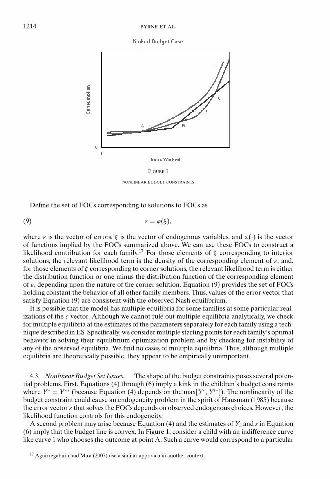
FIGURE 1
NONLINEAR BUDGET CONSTRAINTS
Define the set of FOCs corresponding to solutions to FOCs as
ε = ϕ(ξ),(9)
where ε is the vector of errors, ξ is the vector of endogenous variables, and ϕ(·) is the vectorof functions implied by the FOCs summarized above. We can use these FOCs to construct alikelihood contribution for each family.17 For those elements of ξ corresponding to interiorsolutions, the relevant likelihood term is the density of the corresponding element of ε, and,for those elements of ξ corresponding to corner solutions, the relevant likelihood term is eitherthe distribution function or one minus the distribution function of the corresponding elementof ε, depending upon the nature of the corner solution. Equation (9) provides the set of FOCsholding constant the behavior of all other family members. Thus, values of the error vector thatsatisfy Equation (9) are consistent with the observed Nash equilibrium.
It is possible that the model has multiple equilibria for some families at some particular real-izations of the ε vector. Although we cannot rule out multiple equilibria analytically, we checkfor multiple equilibria at the estimates of the parameters separately for each family using a tech-nique described in ES. Specifically, we consider multiple starting points for each family’s optimalbehavior in solving their equilibrium optimization problem and by checking for instability ofany of the observed equilibria. We find no cases of multiple equilibria. Thus, although multipleequilibria are theoretically possible, they appear to be empirically unimportant.
4.3. Nonlinear Budget Set Issues. The shape of the budget constraints poses several poten-tial problems. First, Equations (4) through (6) imply a kink in the children’s budget constraintswhere Y∗ = Y∗∗ (because Equation (4) depends on the max[Y∗, Y∗∗]). The nonlinearity of thebudget constraint could cause an endogeneity problem in the spirit of Hausman (1985) becausethe error vector ε that solves the FOCs depends on observed endogenous choices. However, thelikelihood function controls for this endogeneity.
A second problem may arise because Equation (4) and the estimates of Yi and s in Equation(6) imply that the budget line is convex. In Figure 1, consider a child with an indifference curvelike curve 1 who chooses the outcome at point A. Such a curve would correspond to a particular
17 Aguirregabiria and Mira (2007) use a similar approach in another context.
FAMILIES’ ELDER CARE DECISIONS 1215
realization of the ε vector. However, if the child had a realization of the ε vector resulting in curve2, any point between B and C would be preferable to point A. We need to rule out situationssimilar to curve 2 in Figure 1.
Third, we observe children at corner solutions. For these children, there must be no valueof the errors satisfying the inequalities in the relevant FOCs that cause the child to move toa different segment of the budget constraint. The leading case for such a problem is a childproviding no financial help for formal care. This implies that εXi must be greater than equationTH
i . Theoretically, for large enough εXi, the value of consumption would increase, possiblycausing the child to move from a budget segment with low hours of work to one with high hoursof work. However, as εXi increases, εLi can increase to keep the child (and her spouse) on theobserved budget segment.
We used the estimated parameter vector (displayed in Table 8) to measure the empiricalimportance of the second and third potential problem. For each child in each family at aninterior solution, we computed the value of ε consistent with the observed choice. For each childin each family at a corner solution, we simulated 10 values of ε consistent with the observedchoice. Conditional on ε, we allowed the child to optimize over all of her choice variables. Wecounted the number of times that the child chose something other than the observed choice.Over the 335,700 choices made, there were no deviations between observed choices and optimalchoices conditional on ε. Thus, although there may be a theoretical problem caused by kinkedbudget sets, it is not an important problem empirically.
5. DATA
We use the 1993 wave of the AHEAD data set to estimate our model. AHEAD is a nationallyrepresentative longitudinal data set designed to facilitate study of Americans aged 70 and older.Its emphasis on the joint dynamics of health, family characteristics, income, and wealth makesit a particularly rich source of information on families’ decisions concerning care for elderlyrelatives, especially in light of its high response rate (over 80%). Although the 1993 wave containsonly noninstitutionalized individuals, the exclusion of nursing home residents is not terriblyproblematic given our focus on informal and formal home health care. Moreover, althoughAHEAD oversamples blacks, Hispanics, and Florida residents, this oversampling causes noestimation bias because our analysis treats race/ethnicity and residential location as exogenous.
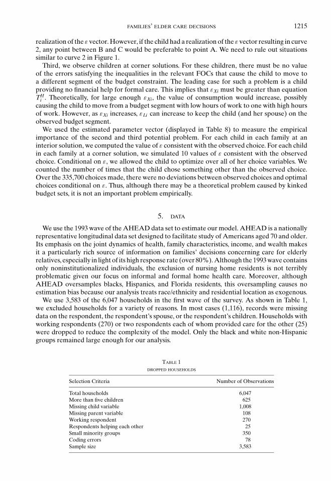
We use 3,583 of the 6,047 households in the first wave of the survey. As shown in Table 1,we excluded households for a variety of reasons. In most cases (1,116), records were missingdata on the respondent, the respondent’s spouse, or the respondent’s children. Households withworking respondents (270) or two respondents each of whom provided care for the other (25)were dropped to reduce the complexity of the model. Only the black and white non-Hispanicgroups remained large enough for our analysis.
TABLE 1DROPPED HOUSEHOLDS
Selection Criteria Number of Observations
Total households 6,047More than five children 625Missing child variable 1,008Missing parent variable 108Working respondent 270Respondents helping each other 25Small minority groups 350Coding errors 78Sample size 3,583
1216 BYRNE ET AL.
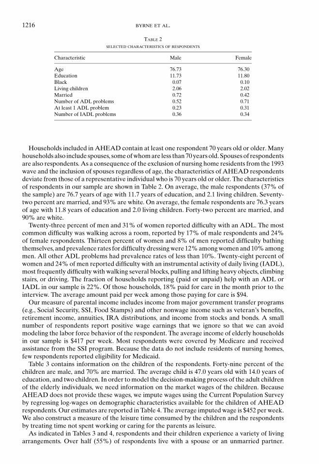
TABLE 2SELECTED CHARACTERISTICS OF RESPONDENTS
Characteristic Male Female
Age 76.73 76.30Education 11.73 11.80Black 0.07 0.10Living children 2.06 2.02Married 0.72 0.42Number of ADL problems 0.52 0.71At least 1 ADL problem 0.23 0.31Number of IADL problems 0.36 0.34
Households included in AHEAD contain at least one respondent 70 years old or older. Manyhouseholds also include spouses, some of whom are less than 70 years old. Spouses of respondentsare also respondents. As a consequence of the exclusion of nursing home residents from the 1993wave and the inclusion of spouses regardless of age, the characteristics of AHEAD respondentsdeviate from those of a representative individual who is 70 years old or older. The characteristicsof respondents in our sample are shown in Table 2. On average, the male respondents (37% ofthe sample) are 76.7 years of age with 11.7 years of education, and 2.1 living children. Seventy-two percent are married, and 93% are white. On average, the female respondents are 76.3 yearsof age with 11.8 years of education and 2.0 living children. Forty-two percent are married, and90% are white.
Twenty-three percent of men and 31% of women reported difficulty with an ADL. The mostcommon difficulty was walking across a room, reported by 17% of male respondents and 24%of female respondents. Thirteen percent of women and 8% of men reported difficulty bathingthemselves, and prevalence rates for difficulty dressing were 12% among women and 10% amongmen. All other ADL problems had prevalence rates of less than 10%. Twenty-eight percent ofwomen and 24% of men reported difficulty with an instrumental activity of daily living (IADL),most frequently difficulty with walking several blocks, pulling and lifting heavy objects, climbingstairs, or driving. The fraction of households reporting (paid or unpaid) help with an ADL orIADL in our sample is 22%. Of those households, 18% paid for care in the month prior to theinterview. The average amount paid per week among those paying for care is $94.
Our measure of parental income includes income from major government transfer programs(e.g., Social Security, SSI, Food Stamps) and other nonwage income such as veteran’s benefits,retirement income, annuities, IRA distributions, and income from stocks and bonds. A smallnumber of respondents report positive wage earnings that we ignore so that we can avoidmodeling the labor force behavior of the respondent. The average income of elderly householdsin our sample is $417 per week. Most respondents were covered by Medicare and receivedassistance from the SSI program. Because the data do not include residents of nursing homes,few respondents reported eligibility for Medicaid.
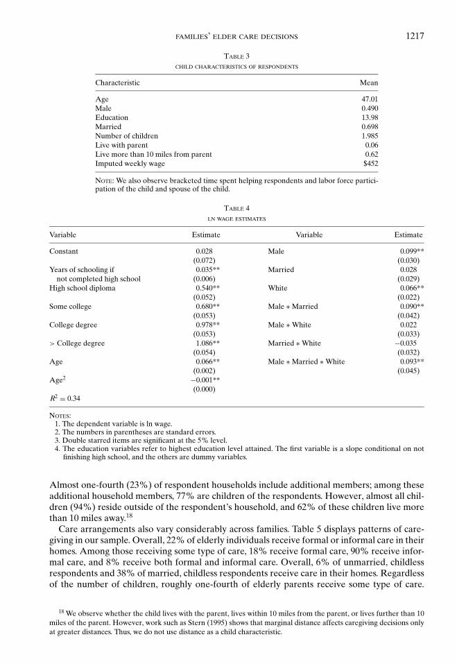
Table 3 contains information on the children of the respondents. Forty-nine percent of thechildren are male, and 70% are married. The average child is 47.0 years old with 14.0 years ofeducation, and two children. In order to model the decision-making process of the adult childrenof the elderly individuals, we need information on the market wages of the children. BecauseAHEAD does not provide these wages, we impute wages using the Current Population Surveyby regressing log-wages on demographic characteristics available for the children of AHEADrespondents. Our estimates are reported in Table 4. The average imputed wage is $452 per week.We also construct a measure of the leisure time consumed by the children and the respondentsby treating time not spent working or caring for the parents as leisure.
As indicated in Tables 3 and 4, respondents and their children experience a variety of livingarrangements. Over half (55%) of respondents live with a spouse or an unmarried partner.
FAMILIES’ ELDER CARE DECISIONS 1217
TABLE 3CHILD CHARACTERISTICS OF RESPONDENTS
Characteristic Mean
Age 47.01Male 0.490Education 13.98Married 0.698Number of children 1.985Live with parent 0.06Live more than 10 miles from parent 0.62Imputed weekly wage $452
NOTE: We also observe bracketed time spent helping respondents and labor force partici-pation of the child and spouse of the child.
TABLE 4LN WAGE ESTIMATES
Variable Estimate Variable Estimate
Constant 0.028 Male 0.099**(0.072) (0.030)
Years of schooling if 0.035** Married 0.028not completed high school (0.006) (0.029)
High school diploma 0.540** White 0.066**(0.052) (0.022)
Some college 0.680** Male ∗ Married 0.090**(0.053) (0.042)
College degree 0.978** Male ∗ White 0.022(0.053) (0.033)
> College degree 1.086** Married ∗ White −0.035(0.054) (0.032)
Age 0.066** Male ∗ Married ∗ White 0.093**(0.002) (0.045)
Age2 −0.001**(0.000)
R2 = 0.34
NOTES:1. The dependent variable is ln wage.2. The numbers in parentheses are standard errors.3. Double starred items are significant at the 5% level.4. The education variables refer to highest education level attained. The first variable is a slope conditional on not
finishing high school, and the others are dummy variables.
Almost one-fourth (23%) of respondent households include additional members; among theseadditional household members, 77% are children of the respondents. However, almost all chil-dren (94%) reside outside of the respondent’s household, and 62% of these children live morethan 10 miles away.18
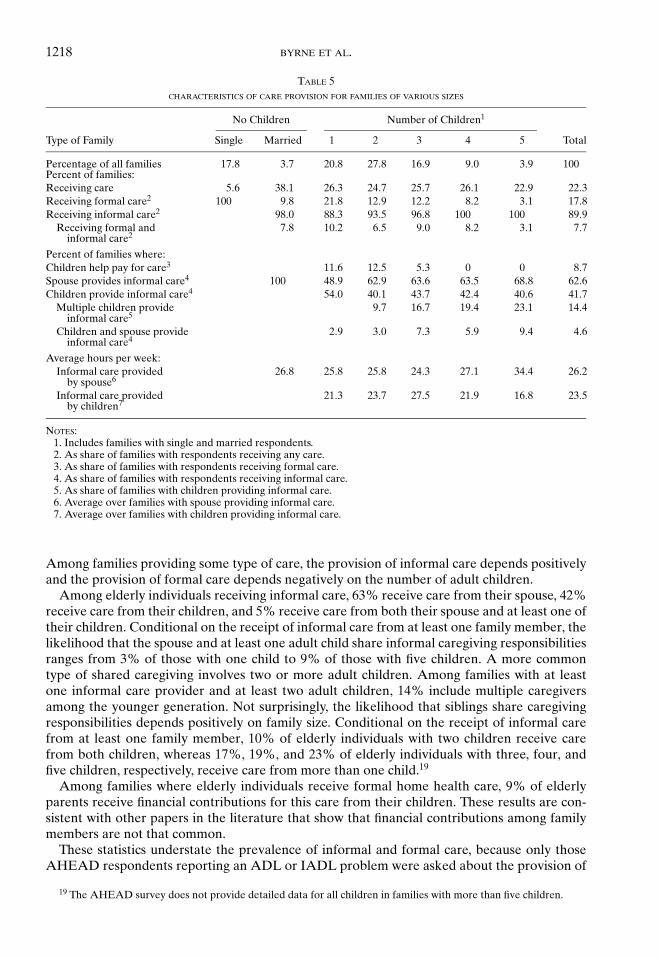
Care arrangements also vary considerably across families. Table 5 displays patterns of care-giving in our sample. Overall, 22% of elderly individuals receive formal or informal care in theirhomes. Among those receiving some type of care, 18% receive formal care, 90% receive infor-mal care, and 8% receive both formal and informal care. Overall, 6% of unmarried, childlessrespondents and 38% of married, childless respondents receive care in their homes. Regardlessof the number of children, roughly one-fourth of elderly parents receive some type of care.
18 We observe whether the child lives with the parent, lives within 10 miles from the parent, or lives further than 10miles of the parent. However, work such as Stern (1995) shows that marginal distance affects caregiving decisions onlyat greater distances. Thus, we do not use distance as a child characteristic.
1218 BYRNE ET AL.
TABLE 5CHARACTERISTICS OF CARE PROVISION FOR FAMILIES OF VARIOUS SIZES
No Children Number of Children1
Type of Family Single Married 1 2 3 4 5 Total
Percentage of all families 17.8 3.7 20.8 27.8 16.9 9.0 3.9 100Percent of families:Receiving care 5.6 38.1 26.3 24.7 25.7 26.1 22.9 22.3Receiving formal care2 100 9.8 21.8 12.9 12.2 8.2 3.1 17.8Receiving informal care2 98.0 88.3 93.5 96.8 100 100 89.9
Receiving formal and 7.8 10.2 6.5 9.0 8.2 3.1 7.7informal care2
Percent of families where:Children help pay for care3 11.6 12.5 5.3 0 0 8.7Spouse provides informal care4 100 48.9 62.9 63.6 63.5 68.8 62.6Children provide informal care4 54.0 40.1 43.7 42.4 40.6 41.7
Multiple children provide 9.7 16.7 19.4 23.1 14.4informal care5
Children and spouse provide 2.9 3.0 7.3 5.9 9.4 4.6informal care4
Average hours per week:Informal care provided 26.8 25.8 25.8 24.3 27.1 34.4 26.2
by spouse6
Informal care provided 21.3 23.7 27.5 21.9 16.8 23.5by children7
NOTES:1. Includes families with single and married respondents.2. As share of families with respondents receiving any care.3. As share of families with respondents receiving formal care.4. As share of families with respondents receiving informal care.5. As share of families with children providing informal care.6. Average over families with spouse providing informal care.7. Average over families with children providing informal care.
Among families providing some type of care, the provision of informal care depends positivelyand the provision of formal care depends negatively on the number of adult children.
Among elderly individuals receiving informal care, 63% receive care from their spouse, 42%receive care from their children, and 5% receive care from both their spouse and at least one oftheir children. Conditional on the receipt of informal care from at least one family member, thelikelihood that the spouse and at least one adult child share informal caregiving responsibilitiesranges from 3% of those with one child to 9% of those with five children. A more commontype of shared caregiving involves two or more adult children. Among families with at leastone informal care provider and at least two adult children, 14% include multiple caregiversamong the younger generation. Not surprisingly, the likelihood that siblings share caregivingresponsibilities depends positively on family size. Conditional on the receipt of informal carefrom at least one family member, 10% of elderly individuals with two children receive carefrom both children, whereas 17%, 19%, and 23% of elderly individuals with three, four, andfive children, respectively, receive care from more than one child.19
Among families where elderly individuals receive formal home health care, 9% of elderlyparents receive financial contributions for this care from their children. These results are con-sistent with other papers in the literature that show that financial contributions among familymembers are not that common.
These statistics understate the prevalence of informal and formal care, because only thoseAHEAD respondents reporting an ADL or IADL problem were asked about the provision of
19 The AHEAD survey does not provide detailed data for all children in families with more than five children.
FAMILIES’ ELDER CARE DECISIONS 1219
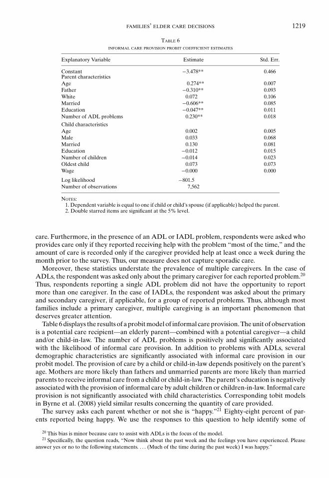
TABLE 6INFORMAL CARE PROVISION PROBIT COEFFICIENT ESTIMATES
Explanatory Variable Estimate Std. Err.
Constant −3.478** 0.466Parent characteristicsAge 0.274** 0.007Father −0.310** 0.093White 0.072 0.106Married −0.606** 0.085Education −0.047** 0.011Number of ADL problems 0.230** 0.018
Child characteristicsAge 0.002 0.005Male 0.033 0.068Married 0.130 0.081Education −0.012 0.015Number of children −0.014 0.023Oldest child 0.073 0.073Wage −0.000 0.000
Log likelihood −801.5Number of observations 7,562
NOTES:1. Dependent variable is equal to one if child or child’s spouse (if applicable) helped the parent.2. Double starred items are significant at the 5% level.
care. Furthermore, in the presence of an ADL or IADL problem, respondents were asked whoprovides care only if they reported receiving help with the problem “most of the time,” and theamount of care is recorded only if the caregiver provided help at least once a week during themonth prior to the survey. Thus, our measure does not capture sporadic care.
Moreover, these statistics understate the prevalence of multiple caregivers. In the case ofADLs, the respondent was asked only about the primary caregiver for each reported problem.20
Thus, respondents reporting a single ADL problem did not have the opportunity to reportmore than one caregiver. In the case of IADLs, the respondent was asked about the primaryand secondary caregiver, if applicable, for a group of reported problems. Thus, although mostfamilies include a primary caregiver, multiple caregiving is an important phenomenon thatdeserves greater attention.
Table 6 displays the results of a probit model of informal care provision. The unit of observationis a potential care recipient—an elderly parent—combined with a potential caregiver—a childand/or child-in-law. The number of ADL problems is positively and significantly associatedwith the likelihood of informal care provision. In addition to problems with ADLs, severaldemographic characteristics are significantly associated with informal care provision in ourprobit model. The provision of care by a child or child-in-law depends positively on the parent’sage. Mothers are more likely than fathers and unmarried parents are more likely than marriedparents to receive informal care from a child or child-in-law. The parent’s education is negativelyassociated with the provision of informal care by adult children or children-in-law. Informal careprovision is not significantly associated with child characteristics. Corresponding tobit modelsin Byrne et al. (2008) yield similar results concerning the quantity of care provided.
The survey asks each parent whether or not she is “happy.”21 Eighty-eight percent of par-ents reported being happy. We use the responses to this question to help identify some of
20 This bias is minor because care to assist with ADLs is the focus of the model.21 Specifically, the question reads, “Now think about the past week and the feelings you have experienced. Please
answer yes or no to the following statements. . . . (Much of the time during the past week) I was happy.”
1220 BYRNE ET AL.
the parameters in our structural model. Identification is discussed in more detail later. A pro-bit model in Byrne et al. (2008) indicates that married individuals are more likely to respondaffirmatively to this question than are unmarried individuals, men are more likely to respond af-firmatively than are women, and whites are more likely to respond affirmatively than are blacks.Moreover, years of education are positively associated with happiness, whereas the number ofADL problems is negatively associated with happiness.
Finally, we construct a number of state-specific variables. These variables include a pricelevel (Bureau of Economic Analysis, 1999), the cost of home health care,22 and the av-erage home health care state subsidy (US. Department of Health and Human Services,1992).
6. ESTIMATION STRATEGY
6.1. Empirical Specification. In order to complete the specification of the model, wespecify the variation of “parameters” across individuals within a family and the joint den-sity of the errors. First, assume that αjik in Equation (1) is a function of parent and childcharacteristics,
α j ik =
exp{W 0
jδ∗α + W 0
kδ∗∗α
}if i = 0
exp{W 0
jδ∗α + Wikδ
∗∗∗α
}if i > 0,
(10)
where W 0j is a vector of parent j ( j = m, p) characteristics, W0
k is a vector of characteristics of thespouse (i.e., k �= j), and Wik is a vector of child characteristics for child i (k = c) and her spouse(k = s). Also, assume that log µ is a constant, and the Zj terms in Equation (1) are functions ofparent characteristics,
Zj = exp{W 0
jδz}.(11)
Next, assume that, in Equations (2) and (3), log β10, log β20, and β30k are constant across families(with β30k = 1), that log β1i (=log β11), log β2i (=log β21), and log β3ik (=log β31) for i > 0 areconstant across families and children within each family, and that
β4 j ik =
W0jkδ
∗β4 + W 0
kδ∗∗β4 if i = 0
Wjikδ∗∗∗β4 + Wikδ
∗∗∗∗β4 if i > 0
.(12)
The terms β30k and β4 j0k cannot be identified separately (except perhaps by functional form)because a parent’s leisure time is determined jointly with her caregiving time. Thus, we set β30k =1 with no loss in generality. Also increasing the constant term in each β term simultaneouslyhas no effect on the FOCs . Thus, we set β2i = 1. For the joint density of the errors, weassume
22 We used two sources of data, Census (1990) and Bureau of Labor Statistics (1998), to interpolate wages for homehealth aid workers in 1993.
FAMILIES’ ELDER CARE DECISIONS 1221
εXi = exp{ηXi },ηXi ∼ i idN
(0, σ 2
ηX
),
εLik ={
exp {ηLik} for i > 0
1 for i = 0,
(ηLic
ηLis
)∼ i idN
(0, σ 2
ηL
(1 ρL
ρL 1
)),
(εt j ic
εt j is
)∼ i idN
(0, σ 2
ηt
(1 ρt
ρt 1
)),
εt j0k ∼ i idN(0, σ 2
ηt
)for j �= k = m, p,
εui ∼ i idN(0, σ 2
u
).
(13)
Based on preliminary results and economic intuition, we restricted the effects of many pa-rameters in order to estimate the effects of the explanatory variables. In general, we restricteda parameter using economic reasoning if, after controlling for the relevant actions, the charac-teristic would not be expected to influence the health production function or utility function inthe manner indicated by the parameter. For example, we would not expect the education of thechild to affect how much the child enjoys caring for her parent, after controlling for the amountof care provided; therefore we restrict the child education characteristic corresponding to theparameter δ∗∗∗∗
β4 (see Equation (12)). In contrast, the number of ADL problems experiencedby the parent probably influences the parent’s utility associated with caregiving; thus we donot restrict the number of ADLs characteristic corresponding to the parameter δ∗
β4. We cannotidentify the constant terms in δ∗
α separately from δ∗∗α or δ∗∗∗
α ; hence, we restrict the constant termsfor δ∗∗
α and δ∗∗∗α .
6.2. The Likelihood Function. The set of parameters to estimate is
θ = (δα, log µ, δz, β0, log β10, log β20, log β11, log β21, log β31, δβ4,
γ, σ 2ηX, σ 2
ηL, σ 2ηt , σ
2u , ρη, ρt
),
(14)
and the set of data for observation n = 1, 2, . . , N is
{[tmik, tpik, Lik, wik, Wi , aik]k∈c,s , Hi , Yi , pXi
}In
i=1
and
{tm0p, tp0m, H0, H, u0, Y0, pX0, q, W 0
m, W 0p, a0p, a0m
}.
The variable t jik is time spent caring for parent j by family member ik. As a result of data issues,we measure time in fractions of a week and we use a discrete measure of t jik in computing thelikelihood function. Its construction is discussed in the Appendix. The variable Hi = 1 iff playeri paid for care:23
Hi = 1 (Hi > 0) .
23 The data do not provide enough information to actually determine if H0 = 1. We assume that, if paid care isprovided, then some of it is paid for by the parents, causing H0 = 1.
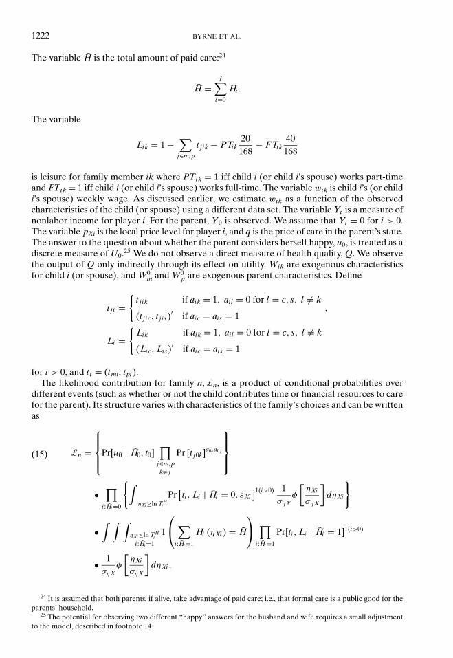
1222 BYRNE ET AL.
The variable H is the total amount of paid care:24
H =I∑
i=0
Hi .
The variable
Lik = 1 −∑
j∈m,p
t jik − PTik20168
− FTik40
168
is leisure for family member ik where PTik = 1 iff child i (or child i’s spouse) works part-timeand FTik = 1 iff child i (or child i’s spouse) works full-time. The variable wik is child i’s (or childi’s spouse) weekly wage. As discussed earlier, we estimate wik as a function of the observedcharacteristics of the child (or spouse) using a different data set. The variable Yi is a measure ofnonlabor income for player i. For the parent, Y0 is observed. We assume that Yi = 0 for i > 0.The variable pXi is the local price level for player i, and q is the price of care in the parent’s state.The answer to the question about whether the parent considers herself happy, u0, is treated as adiscrete measure of U0.25 We do not observe a direct measure of health quality, Q. We observethe output of Q only indirectly through its effect on utility. Wik are exogenous characteristicsfor child i (or spouse), and W0
m and W0p are exogenous parent characteristics. Define
t ji ={
t jik if aik = 1, ail = 0 for l = c, s, l �= k
(t jic, t jis)′ if aic = ais = 1,
Li ={
Lik if aik = 1, ail = 0 for l = c, s, l �= k
(Lic, Lis)′ if aic = ais = 1
for i > 0, and t i = (tmi, tpi ).The likelihood contribution for family n, £n, is a product of conditional probabilities over
different events (such as whether or not the child contributes time or financial resources to carefor the parent). Its structure varies with characteristics of the family’s choices and can be writtenas
£n =
Pr[u0 | H0, t0]
∏j∈m,pk�= j
Pr [t j0k]a0ka0 j
•∏
i :Hi =0
{∫ηXi ≥ln TH
i
Pr[ti , Li | Hi = 0, εXi
]1(i>0) 1σηX
φ
[ηXi
σηX
]dηXi
}
•∫ ∫ ∫
ηXi ≤ln THi
i :Hi =1
1
∑
i :Hi =1
Hi (ηXi ) = H
∏
i :Hi =1
Pr[ti , Li | Hi = 1]1(i>0)
• 1σηX
φ
[ηXi
σηX
]dηXi ,
(15)
24 It is assumed that both parents, if alive, take advantage of paid care; i.e., that formal care is a public good for theparents’ household.
25 The potential for observing two different “happy” answers for the husband and wife requires a small adjustmentto the model, described in footnote 14.
FAMILIES’ ELDER CARE DECISIONS 1223
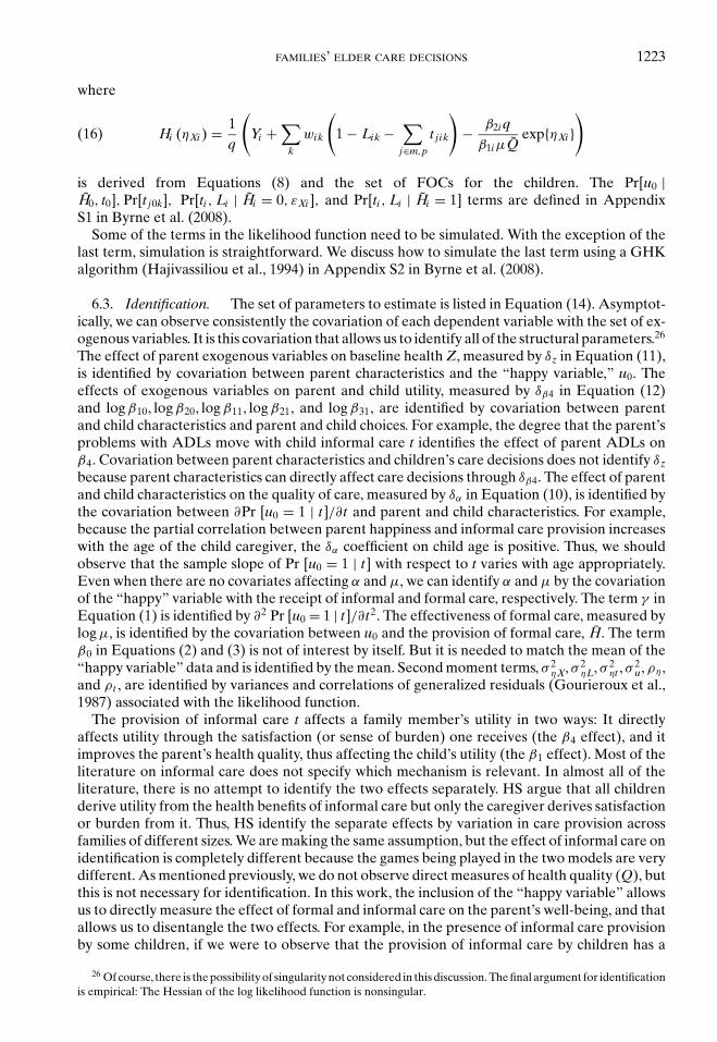
where
Hi (ηXi ) = 1q
(Yi +
∑k
wik
(1 − Lik −
∑j∈m,p
t jik
)− β2i q
β1iµQexp{ηXi }
)(16)
is derived from Equations (8) and the set of FOCs for the children. The Pr[u0 |H0, t0], Pr[t j0k], Pr[ti , Li | Hi = 0, εXi ], and Pr[ti , Li | Hi = 1] terms are defined in AppendixS1 in Byrne et al. (2008).
Some of the terms in the likelihood function need to be simulated. With the exception of thelast term, simulation is straightforward. We discuss how to simulate the last term using a GHKalgorithm (Hajivassiliou et al., 1994) in Appendix S2 in Byrne et al. (2008).
6.3. Identification. The set of parameters to estimate is listed in Equation (14). Asymptot-ically, we can observe consistently the covariation of each dependent variable with the set of ex-ogenous variables. It is this covariation that allows us to identify all of the structural parameters.26
The effect of parent exogenous variables on baseline health Z, measured by δz in Equation (11),is identified by covariation between parent characteristics and the “happy variable,” u0. Theeffects of exogenous variables on parent and child utility, measured by δβ4 in Equation (12)and log β10, log β20, log β11, log β21, and log β31, are identified by covariation between parentand child characteristics and parent and child choices. For example, the degree that the parent’sproblems with ADLs move with child informal care t identifies the effect of parent ADLs onβ4. Covariation between parent characteristics and children’s care decisions does not identify δz
because parent characteristics can directly affect care decisions through δβ4. The effect of parentand child characteristics on the quality of care, measured by δα in Equation (10), is identified bythe covariation between ∂Pr [u0 = 1 | t]/∂t and parent and child characteristics. For example,because the partial correlation between parent happiness and informal care provision increaseswith the age of the child caregiver, the δα coefficient on child age is positive. Thus, we shouldobserve that the sample slope of Pr [u0 = 1 | t] with respect to t varies with age appropriately.Even when there are no covariates affecting α and µ, we can identify α and µ by the covariationof the “happy” variable with the receipt of informal and formal care, respectively. The term γ inEquation (1) is identified by ∂2 Pr [u0 = 1 | t]/∂t2. The effectiveness of formal care, measured bylog µ, is identified by the covariation between u0 and the provision of formal care, H. The termβ0 in Equations (2) and (3) is not of interest by itself. But it is needed to match the mean of the“happy variable” data and is identified by the mean. Second moment terms, σ 2
ηX, σ 2ηL, σ 2
ηt , σ2u, ρη,
and ρ t , are identified by variances and correlations of generalized residuals (Gourieroux et al.,1987) associated with the likelihood function.
The provision of informal care t affects a family member’s utility in two ways: It directlyaffects utility through the satisfaction (or sense of burden) one receives (the β4 effect), and itimproves the parent’s health quality, thus affecting the child’s utility (the β1 effect). Most of theliterature on informal care does not specify which mechanism is relevant. In almost all of theliterature, there is no attempt to identify the two effects separately. HS argue that all childrenderive utility from the health benefits of informal care but only the caregiver derives satisfactionor burden from it. Thus, HS identify the separate effects by variation in care provision acrossfamilies of different sizes. We are making the same assumption, but the effect of informal care onidentification is completely different because the games being played in the two models are verydifferent. As mentioned previously, we do not observe direct measures of health quality (Q), butthis is not necessary for identification. In this work, the inclusion of the “happy variable” allowsus to directly measure the effect of formal and informal care on the parent’s well-being, and thatallows us to disentangle the two effects. For example, in the presence of informal care provisionby some children, if we were to observe that the provision of informal care by children has a
26 Of course, there is the possibility of singularity not considered in this discussion. The final argument for identificationis empirical: The Hessian of the log likelihood function is nonsingular.
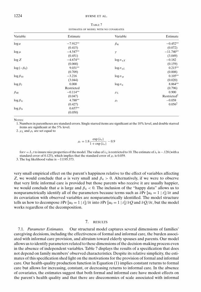
1224 BYRNE ET AL.
TABLE 7ESTIMATES OF MODEL WITH NO COVARIATES
Variable Estimate Variable Estimate
log α −7.912∗∗ β4i −0.452∗∗(0.415) (0.072)
log µ −4.547∗∗ γ −11.740∗∗(0.451) (3.049)
log Z −4.674∗∗ log σηX −0.182(0.068) (0.159)
log (−β0) 9.031∗∗ log σηL 0.215∗∗(0.709) (0.008)
log β10 −3.216 log σηt 0.105∗∗(3.044) (0.020)
log β2 0.000 log σ u 8.864∗∗Restricted (0.796)
β40 −0.114∗∗ ρL 0.900(0.047) Restricted2
log β1i 4.788∗∗ ρt −0.058(0.427) 0.0562
log β3i 0.657∗∗(0.050)
NOTES:1. Numbers in parentheses are standard errors. Single starred items are significant at the 10% level, and double starred
items are significant at the 5% level.2. ρL and ρt are set equal to
ρr = 1.8exp {λr }
1 + exp {λr } − 0.9
for r = L, t to insure nice properties of the model. The value of λL is restricted to 10. The estimate of λt is −.128 (with astandard error of 0.125), which implies that the standard error of ρt is 0.059.
3. The log likelihood value is −11195.373.
very small empirical effect on the parent’s happiness relative to the effect of variables affectingZ, we would conclude that α is very small and β4 > 0. Alternatively, if we were to observethat very little informal care is provided but those parents who receive it are usually happier,we would conclude that α is large and β4 < 0. The inclusion of the “happy data” allows us tononparametrically identify all of the parameters because terms such as ∂Pr [u0 = 1 | t]/∂t andits covariation with observed variables are nonparametrically identified. The model structuretells us how to decompose ∂Pr [u0 = 1 | t]/∂t into ∂Pr [u0 = 1 | t]/∂ Q and ∂ Q/∂t , but the modelworks regardless of the decomposition.
7. RESULTS
7.1. Parameter Estimates. Our structural model captures several dimensions of families’caregiving decisions, including the effectiveness of formal and informal care, the burden associ-ated with informal care provision, and altruism toward elderly spouses and parents. Our modelallows us to identify parameters related to these dimensions of the decision-making process evenin the absence of independent variables. Table 7 displays the results of a specification that doesnot depend on family members’ observed characteristics. Despite its relative simplicity, the esti-mates of this specification shed light on the motivations for the provision of formal and informalcare. Our health-quality production function in Equation (1) implies constant returns to formalcare but allows for increasing, constant, or decreasing returns to informal care. In the absenceof covariates, the estimates suggest that both formal and informal care have modest effects onthe parent’s health quality and that there are diseconomies of scale associated with informal
FAMILIES’ ELDER CARE DECISIONS 1225
care. Moreover, the estimates suggests that not only is informal care relatively ineffective butits provision tends to be burdensome. These results may explain why few family members pro-vide care for elderly individuals. However, the results of this simple version of the model implythat adult children and children-in-law care about their parents’ health quality, suggesting thataltruism may play an important role in the provision of informal and formal care.
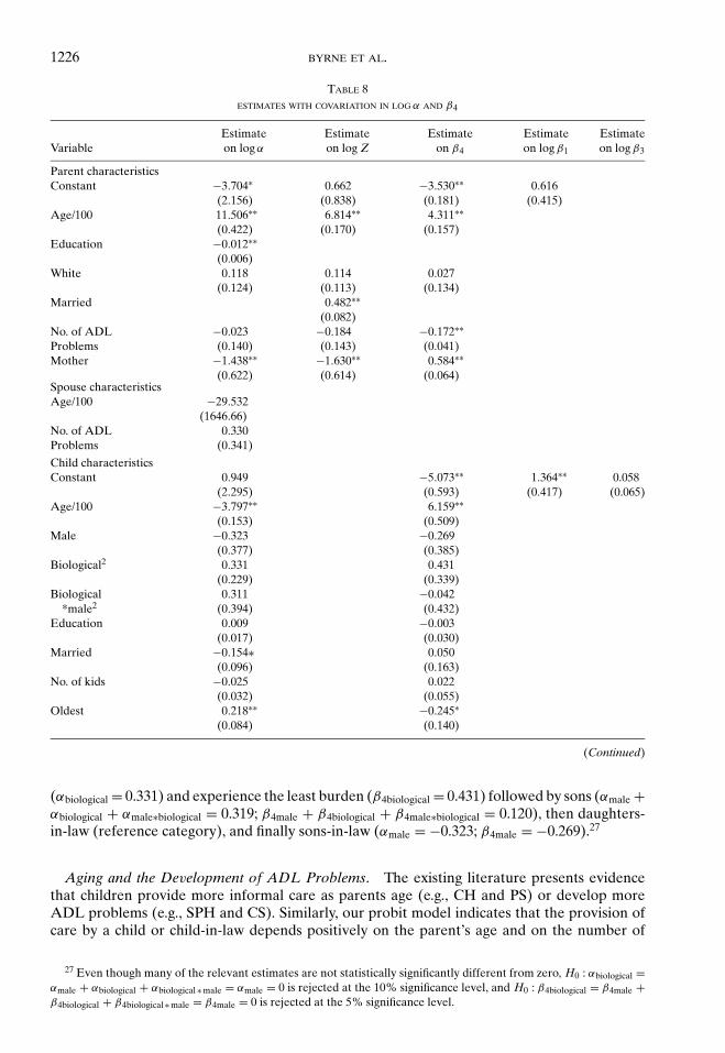
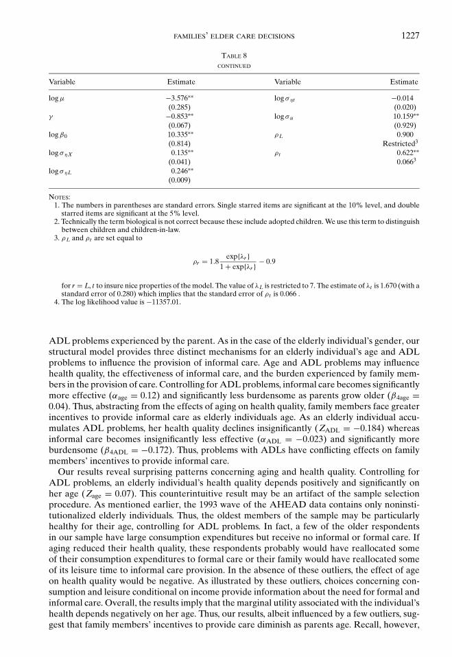
Another version of our model allows the α and Z terms in Equation (1) and the β4 termin Equations (2) and (3) to depend on covariates. This specification allows family members’characteristics to affect both the quality of care provided and the burden associated with care-giving. In addition, this specification allows elderly individuals’ characteristics to affect theirhealth quality and, in turn, all family members’ utility. A child or child-in-law’s provision ofcare depends on the parent’s health quality, the effectiveness of informal care, and the burdenassociated with caregiving. An elderly individual’s utility depends on the effectiveness of carebut not on her children’s caregiving burden. Thus, we can identify the effect of characteristicssuch as the parent’s age on the burden associated with informal care provision from the effect ofthe same characteristic on the quality of informal care. Table 8 presents the results of our modelwith covariates, and Table 9 displays the first two moments of relevant model characteristics. Alikelihood-ratio test rejects the model without covariates in favor of the model with covariates.
Gender. Our structural model provides three distinct mechanisms for an elderly individual’sgender to influence the provision of informal care. Specifically, our model allows for the possi-bility that health quality, the effectiveness of informal care, and the burden associated with itsprovision differ for elderly men and women. Controlling for age, race, marital status, and thenumber of ADL problems, our results suggest that elderly men experience significantly greaterhealth quality than do elderly women prior to any formal or informal care decisions (Zmother =−1.630). Thus, the marginal utility associated with the mother’s health quality exceeds themarginal utility associated with the father’s health quality. In turn, children face greater incen-tives to provide care for mothers than for fathers, abstracting from the effects of gender on thequality of care and the burden associated with its provision. Moreover, our results suggest thatinformal care provided to mothers (wives) is significantly less burdensome than care provided tofathers (husbands) (β4mother = 0.584), again providing children with greater incentive to spendtime caring for elderly mothers than fathers. Similarly, our probit results of informal care pro-vision indicate that mothers are significantly more likely than fathers to receive informal carefrom children or children-in-law, and HS report that families value care provided for mothersmore than care provided for fathers. However, the results of our structural model suggest thatinformal care provided to mothers (wives) is significantly less effective (αmother = −1.438) thaninformal care provided to fathers (husbands). This gender difference may shed light on PS’ find-ing that daughters are more likely to provide care for fathers than mothers. Overall the resultsof our structural model suggest that elderly women may have greater caregiving needs thando elderly men; although care provided to mothers is significantly less burdensome than careprovided to fathers, it is significantly less effective. The complex relationship between genderand motives for informal care provision may contribute to the conflicting evidence presented inthe literature.
Child gender also plays a role in family caregiving. ES, CS, and SPH find that, all else equal,daughters are significantly more likely than sons to provide care, whereas SPH’s findings indicatethat sons provide significantly more care than do daughters. Our structural model allows boththe effectiveness of informal care and the burden associated with its provision to differ by childgender. The model also distinguishes between children and children-in-law. In our raw data,7.0% of daughters provide informal care, compared to 4.0% of sons, 1.6% of daughters-in-law, and 0.8% of sons-in-law. These differences suggest that the quality of care, the burdenassociated with its provision, and/or opportunity costs may differ by gender; similarly, childrenmay provide higher quality care and experience less burden than their spouses. In fact, theresults of our structural model indicate that children provide higher quality care and experienceless burden than do children-in-law. In particular, daughters provide the highest quality care
1226 BYRNE ET AL.
TABLE 8ESTIMATES WITH COVARIATION IN LOG α AND β4
Estimate Estimate Estimate Estimate EstimateVariable on log α on log Z on β4 on log β1 on log β3
Parent characteristicsConstant −3.704∗ 0.662 −3.530∗∗ 0.616
(2.156) (0.838) (0.181) (0.415)Age/100 11.506∗∗ 6.814∗∗ 4.311∗∗
(0.422) (0.170) (0.157)Education −0.012∗∗
(0.006)White 0.118 0.114 0.027
(0.124) (0.113) (0.134)Married 0.482∗∗
(0.082)No. of ADL −0.023 −0.184 −0.172∗∗Problems (0.140) (0.143) (0.041)Mother −1.438∗∗ −1.630∗∗ 0.584∗∗
(0.622) (0.614) (0.064)Spouse characteristicsAge/100 −29.532
(1646.66)No. of ADL 0.330Problems (0.341)
Child characteristicsConstant 0.949 −5.073∗∗ 1.364∗∗ 0.058
(2.295) (0.593) (0.417) (0.065)Age/100 −3.797∗∗ 6.159∗∗
(0.153) (0.509)Male −0.323 −0.269
(0.377) (0.385)Biological2 0.331 0.431
(0.229) (0.339)Biological 0.311 −0.042
*male2 (0.394) (0.432)Education 0.009 −0.003
(0.017) (0.030)Married −0.154∗ 0.050
(0.096) (0.163)No. of kids −0.025 0.022
(0.032) (0.055)Oldest 0.218∗∗ −0.245∗
(0.084) (0.140)
(Continued)
(αbiological = 0.331) and experience the least burden (β4biological = 0.431) followed by sons (αmale +αbiological + αmale∗biological = 0.319; β4male + β4biological + β4male∗biological = 0.120), then daughters-in-law (reference category), and finally sons-in-law (αmale = −0.323; β4male = −0.269).27
Aging and the Development of ADL Problems. The existing literature presents evidencethat children provide more informal care as parents age (e.g., CH and PS) or develop moreADL problems (e.g., SPH and CS). Similarly, our probit model indicates that the provision ofcare by a child or child-in-law depends positively on the parent’s age and on the number of
27 Even though many of the relevant estimates are not statistically significantly different from zero, H0 : αbiological =αmale + αbiological + αbiological ∗ male = αmale = 0 is rejected at the 10% significance level, and H0 : β4biological = β4male +β4biological + β4biological ∗ male = β4male = 0 is rejected at the 5% significance level.
FAMILIES’ ELDER CARE DECISIONS 1227
TABLE 8CONTINUED
Variable Estimate Variable Estimate
log µ −3.576∗∗ log σηt −0.014(0.285) (0.020)
γ −0.853∗∗ log σ u 10.159∗∗(0.067) (0.929)
log β0 10.335∗∗ ρL 0.900(0.814) Restricted3
log σηX 0.135∗∗ ρt 0.622∗∗(0.041) 0.0663
log σηL 0.246∗∗(0.009)
NOTES:1. The numbers in parentheses are standard errors. Single starred items are significant at the 10% level, and double
starred items are significant at the 5% level.2. Technically the term biological is not correct because these include adopted children. We use this term to distinguish
between children and children-in-law.3. ρL and ρt are set equal to
ρr = 1.8exp{λr }
1 + exp{λr } − 0.9
for r = L, t to insure nice properties of the model. The value of λL is restricted to 7. The estimate of λt is 1.670 (with astandard error of 0.280) which implies that the standard error of ρt is 0.066 .
4. The log likelihood value is −11357.01.
ADL problems experienced by the parent. As in the case of the elderly individual’s gender, ourstructural model provides three distinct mechanisms for an elderly individual’s age and ADLproblems to influence the provision of informal care. Age and ADL problems may influencehealth quality, the effectiveness of informal care, and the burden experienced by family mem-bers in the provision of care. Controlling for ADL problems, informal care becomes significantlymore effective (αage = 0.12) and significantly less burdensome as parents grow older (β4age =0.04). Thus, abstracting from the effects of aging on health quality, family members face greaterincentives to provide informal care as elderly individuals age. As an elderly individual accu-mulates ADL problems, her health quality declines insignificantly (ZADL = −0.184) whereasinformal care becomes insignificantly less effective (αADL = −0.023) and significantly moreburdensome (β4ADL = −0.172). Thus, problems with ADLs have conflicting effects on familymembers’ incentives to provide informal care.
Our results reveal surprising patterns concerning aging and health quality. Controlling forADL problems, an elderly individual’s health quality depends positively and significantly onher age (Zage = 0.07). This counterintuitive result may be an artifact of the sample selectionprocedure. As mentioned earlier, the 1993 wave of the AHEAD data contains only noninsti-tutionalized elderly individuals. Thus, the oldest members of the sample may be particularlyhealthy for their age, controlling for ADL problems. In fact, a few of the older respondentsin our sample have large consumption expenditures but receive no informal or formal care. Ifaging reduced their health quality, these respondents probably would have reallocated someof their consumption expenditures to formal care or their family would have reallocated someof its leisure time to informal care provision. In the absence of these outliers, the effect of ageon health quality would be negative. As illustrated by these outliers, choices concerning con-sumption and leisure conditional on income provide information about the need for formal andinformal care. Overall, the results imply that the marginal utility associated with the individual’shealth depends negatively on her age. Thus, our results, albeit influenced by a few outliers, sug-gest that family members’ incentives to provide care diminish as parents age. Recall, however,
1228 BYRNE ET AL.
that these implications abstract from the effects of aging on the effectiveness of informal careand the burden associated with its provision.
Our model also allows for the spouse’s age and ADL problems to influence the effectivenessof informal care. Neither of these relationships approaches statistical significance.
Children’s Ages and Parity. In addition, our model allows for the age of a child and her parity(whether she is the oldest child) to influence the effectiveness of informal care and the burden as-sociated with its provision. Consistent with the results presented in HS, neither the age of a childnor her parity is significantly associated with the provision of informal care in our probit model.Our structural model reveals a more complex relationship between a child’s age and the provi-sion of informal care, namely, that children provide significantly less effective care (αchildage =−0.04) but experience significantly less burden (β4childage = 0.06) as they age. The reduction inquality may be attributable to diminished health and energy of children as they age, whereasthe reduction in burden may be attributable to the reduced demands on adult children’s timeas their own children reach adulthood and leave home. (Our model controls for an adult child’sfamily size but not the ages of her children.) Controlling for age, our structural model indicatesthat oldest children provide significantly more effective care (αoldest = 0.218) but experiencesignificantly greater burden (β4oldest = −0.245) than their siblings. Thus, an adult child’s age andparity both have ambiguous effects on her incentives to provide informal care.
Marriage and Family Size. An elderly individual’s marital status influences the family’s caredecisions. Consistent with other studies (e.g., HS, ES, CS, and PS), our probit model indicatesthat married individuals are less likely to receive informal care from their children or children-in-law than are unmarried individuals. This result suggests that marriage enhances health and/orthat married individuals are more likely to rely on their spouses than on their children for theprovision of care. Our structural model provides support for both of these explanations. Marriedindividuals enjoy significantly greater health than do their unmarried counterparts prior to anyformal or informal care decisions (Zmarried = 0.482). The model does not directly allow for thepossibility that an elderly individual’s marital status influences the effectiveness of informalcare or the burden associated with its provision. However, the model allows for the quality andburden associated with informal care to differ for spouses and children. Although, on average,children are more effective caregivers than are spouses (the mean log α is greater for childrenthan for spouses), they tend to experience greater burden (the mean β4 is almost 36 times largerfor children than for spouses). This discrepancy in caregiving burden contributes to spouses’greater propensity to provide care. For example, our parameter estimates indicate that, in about80% of families with a married elderly individual and one adult child, the elderly individual’sspouse is more likely than her child and/or child-in-law to provide care.
Adult children’s family structure may also influence care decisions. Our structural modelallows for an adult child’s marital status and family size to influence both the effectiveness ofcare and the burden associated with its provision. Consistent with SPH’s finding that marriedchildren provide less care for their elderly parents than do unmarried children, our resultsindicate that married children provide significantly less effective care (αmarried = 0.154) thantheir unmarried counterparts. However, marital status is not significantly related to caregivingburden. Surprisingly, an adult child’s family size is not significantly related to her caregivingeffectiveness or burden.
Education. Previous studies (e.g., HS and ES) use education as a proxy for income and at-tribute the greater reliance on formal care instead of informal care among more highly educatedindividuals to an income effect. Similarly, our probit model indicates that parental education isnegatively associated with informal care provision by children or children-in-law. In our struc-tural model, family members make caregiving decisions as part of a broader constrained max-imization problem. Thus, our model and data disentangle the effects of income and education.Specifically, our model allows for the possibility that the effectiveness of informal care depends
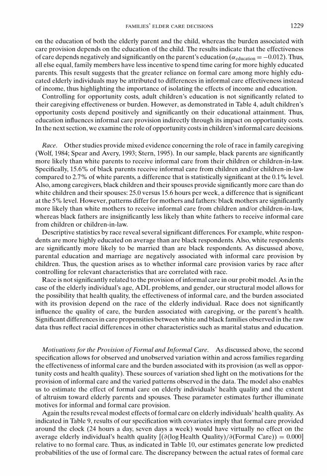
FAMILIES’ ELDER CARE DECISIONS 1229
on the education of both the elderly parent and the child, whereas the burden associated withcare provision depends on the education of the child. The results indicate that the effectivenessof care depends negatively and significantly on the parent’s education (αeducation =−0.012). Thus,all else equal, family members have less incentive to spend time caring for more highly educatedparents. This result suggests that the greater reliance on formal care among more highly edu-cated elderly individuals may be attributed to differences in informal care effectiveness insteadof income, thus highlighting the importance of isolating the effects of income and education.
Controlling for opportunity costs, adult children’s education is not significantly related totheir caregiving effectiveness or burden. However, as demonstrated in Table 4, adult children’sopportunity costs depend positively and significantly on their educational attainment. Thus,education influences informal care provision indirectly through its impact on opportunity costs.In the next section, we examine the role of opportunity costs in children’s informal care decisions.
Race. Other studies provide mixed evidence concerning the role of race in family caregiving(Wolf, 1984; Spear and Avery, 1993; Stern, 1995). In our sample, black parents are significantlymore likely than white parents to receive informal care from their children or children-in-law.Specifically, 15.6% of black parents receive informal care from children and/or children-in-lawcompared to 2.7% of white parents, a difference that is statistically significant at the 0.1% level.Also, among caregivers, black children and their spouses provide significantly more care than dowhite children and their spouses: 25.0 versus 15.6 hours per week, a difference that is significantat the 5% level. However, patterns differ for mothers and fathers: black mothers are significantlymore likely than white mothers to receive informal care from children and/or children-in-law,whereas black fathers are insignificantly less likely than white fathers to receive informal carefrom children or children-in-law.
Descriptive statistics by race reveal several significant differences. For example, white respon-dents are more highly educated on average than are black respondents. Also, white respondentsare significantly more likely to be married than are black respondents. As discussed above,parental education and marriage are negatively associated with informal care provision bychildren. Thus, the question arises as to whether informal care provision varies by race aftercontrolling for relevant characteristics that are correlated with race.
Race is not significantly related to the provision of informal care in our probit model. As in thecase of the elderly individual’s age, ADL problems, and gender, our structural model allows forthe possibility that health quality, the effectiveness of informal care, and the burden associatedwith its provision depend on the race of the elderly individual. Race does not significantlyinfluence the quality of care, the burden associated with caregiving, or the parent’s health.Significant differences in care propensities between white and black families observed in the rawdata thus reflect racial differences in other characteristics such as marital status and education.
Motivations for the Provision of Formal and Informal Care. As discussed above, the secondspecification allows for observed and unobserved variation within and across families regardingthe effectiveness of informal care and the burden associated with its provision (as well as oppor-tunity costs and health quality). These sources of variation shed light on the motivations for theprovision of informal care and the varied patterns observed in the data. The model also enablesus to estimate the effect of formal care on elderly individuals’ health quality and the extentof altruism toward elderly parents and spouses. These parameter estimates further illuminatemotives for informal and formal care provision.
Again the results reveal modest effects of formal care on elderly individuals’ health quality. Asindicated in Table 9, results of our specification with covariates imply that formal care providedaround the clock (24 hours a day, seven days a week) would have virtually no effect on theaverage elderly individual’s health quality [(∂(log Health Quality)/∂(Formal Care)) = 0.000]relative to no formal care. Thus, as indicated in Table 10, our estimates generate low predictedprobabilities of the use of formal care. The discrepancy between the actual rates of formal care
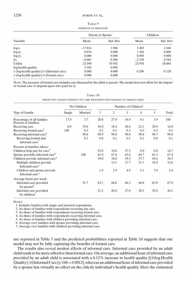
1230 BYRNE ET AL.
TABLE 9MOMENTS OF BEHAVIOR
Parent or Spouse Children
Variable Mean Std. Dev Mean Std. Dev
log α −17.814 1.966 3.403 1.044log β1 0.616 0.000 1.364 0.000log β3 0.000 0.000 0.058 0.000β4 −0.061 0.366 −2.194 0.544Utility 23.590 19.952 23.970 18.065log health quality 5.102 0.984∂ (log health quality)/∂ (informal care) 0.000 0.000 0.206 0.129∂ (log health quality)/∂ (formal care) 0.000 0.000
NOTE: The measure of formal care includes care financed by the child or parent. The model does not allow for the impactof formal care to depend upon who paid for it.
TABLE 10PREDICTED CHARACTERISTICS OF CARE PROVISION FOR FAMILIES OF VARIOUS SIZES
No Children Number of Children1
Type of Family Single Married 1 2 3 4 5 Total
Percentage of all families 17.8 3.7 20.8 27.9 16.9 9.1 3.9 100Percent of families:Receiving care 0.0 33.6 16.0 18.4 20.4 22.1 20.9 16.0Receiving formal care2 100 0.3 0.2 0.3 0.3 0.3 0.3 0.3Receiving informal care2 99.8 99.9 99.8 99.8 99.8 99.7 99.8
Receiving formal and 0.1 0.0 0.1 0.1 0.1 0.0 0.1informal care2
Percent of families where:Children help pay for care3 25.0 10.0 37.5 0.0 0.0 14.7Spouse provides informal care4 100 61.9 67.8 63.6 64.7 61.3 67.4Children provide informal care4 39.0 34.0 39.3 37.7 43.6 34.5
Multiple children provide 13.1 17.7 21.7 16.9 12.6Informal care5
Children and spouse provide 1.9 2.9 4.9 5.1 7.0 3.4Informal care4
Average hours per week:Informal care provided 91.7 63.1 68.8 64.3 66.8 63.9 67.9
by spouse6
Informal care provided 21.2 26.0 27.6 30.3 29.0 26.1by children7
NOTES:1. Includes families with single and married respondents.2. As share of families with respondents receiving any care.3. As share of families with respondents receiving formal care.4. As share of families with respondents receiving informal care.5. As share of families with children providing informal care.6. Average over families with spouse providing informal care.7. Average over families with children providing informal care.
use reported in Table 5 and the predicted probabilities reported in Table 10 suggests that ourmodel may not be fully capturing the benefits of formal care.
The results also reveal modest effects of informal care. Informal care provided by an adultchild tends to be more effective than formal care. On average, an additional hour of informal careprovided by an adult child is associated with a 0.12% increase in health quality [(∂(log HealthQuality)/∂(Informal Care))/168=0.0012], whereas an additional hour of informal care providedby a spouse has virtually no effect on the elderly individual’s health quality. Here the estimated
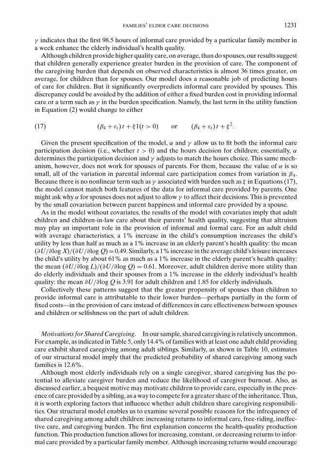
FAMILIES’ ELDER CARE DECISIONS 1231
γ indicates that the first 98.5 hours of informal care provided by a particular family member ina week enhance the elderly individual’s health quality.
Although children provide higher quality care, on average, than do spouses, our results suggestthat children generally experience greater burden in the provision of care. The component ofthe caregiving burden that depends on observed characteristics is almost 36 times greater, onaverage, for children than for spouses. Our model does a reasonable job of predicting hoursof care for children. But it significantly overpredicts informal care provided by spouses. Thisdiscrepancy could be avoided by the addition of either a fixed burden cost in providing informalcare or a term such as γ in the burden specification. Namely, the last term in the utility functionin Equation (2) would change to either
(β4 + εt ) t + ξ1(t > 0) or (β4 + εt ) t + ξ 2.(17)
Given the present specification of the model, α and γ allow us to fit both the informal careparticipation decision (i.e., whether t > 0) and the hours decision for children; essentially, α
determines the participation decision and γ adjusts to match the hours choice. This same mech-anism, however, does not work for spouses of parents. For them, because the value of α is sosmall, all of the variation in parental informal care participation comes from variation in β4.Because there is no nonlinear term such as γ associated with burden such as ξ in Equations (17),the model cannot match both features of the data for informal care provided by parents. Onemight ask why α for spouses does not adjust to allow γ to affect their decisions. This is preventedby the small covariation between parent happiness and informal care provided by a spouse.
As in the model without covariates, the results of the model with covariates imply that adultchildren and children-in-law care about their parents’ health quality, suggesting that altruismmay play an important role in the provision of informal and formal care. For an adult childwith average characteristics, a 1% increase in the child’s consumption increases the child’sutility by less than half as much as a 1% increase in an elderly parent’s health quality: the mean(∂U/∂log X)/(∂U/∂log Q) = 0.49. Similarly, a 1% increase in the average child’s leisure increasesthe child’s utility by about 61% as much as a 1% increase in the elderly parent’s health quality:the mean (∂U/∂log L)/(∂U/∂log Q) = 0.61. Moreover, adult children derive more utility thando elderly individuals and their spouses from a 1% increase in the elderly individual’s healthquality: the mean ∂U/∂log Q is 3.91 for adult children and 1.85 for elderly individuals.
Collectively these patterns suggest that the greater propensity of spouses than children toprovide informal care is attributable to their lower burden—perhaps partially in the form offixed costs—in the provision of care instead of differences in care effectiveness between spousesand children or selfishness on the part of adult children.
Motivations for Shared Caregiving. In our sample, shared caregiving is relatively uncommon.For example, as indicated in Table 5, only 14.4% of families with at least one adult child providingcare exhibit shared caregiving among adult siblings. Similarly, as shown in Table 10, estimatesof our structural model imply that the predicted probability of shared caregiving among suchfamilies is 12.6%.
Although most elderly individuals rely on a single caregiver, shared caregiving has the po-tential to alleviate caregiver burden and reduce the likelihood of caregiver burnout. Also, asdiscussed earlier, a bequest motive may motivate children to provide care, especially in the pres-ence of care provided by a sibling, as a way to compete for a greater share of the inheritance. Thus,it is worth exploring factors that influence whether adult children share caregiving responsibili-ties. Our structural model enables us to examine several possible reasons for the infrequency ofshared caregiving among adult children: increasing returns to informal care, free-riding, ineffec-tive care, and caregiving burden. The first explanation concerns the health-quality productionfunction. This production function allows for increasing, constant, or decreasing returns to infor-mal care provided by a particular family member. Although increasing returns would encourage
1232 BYRNE ET AL.
the reliance on a single caregiver, decreasing returns would encourage shared caregiving. In lightof strong evidence of decreasing returns to informal care provided by a particular family member(γ is significantly less than 0), concerns about the quality of care do not explain the infrequencyof shared caregiving.
The second explanation for the lack of shared caregiving concerns the possibility of free-riding.The infrequency of shared caregiving could be attributable to free-riding if adult siblings’ infor-mal care decisions were negatively correlated (see CS for a discussion of the issue). However, thesimulated informal care decisions of children are nearly independent of one another, suggestingthat free-riding is not prevalent.28 The low correlations between siblings’ care probabilities occurbecause other phenomena such as elderly parents’ preferences for shared caregiving counteractadult children’s incentives to free-ride on one another. More technically, the latent utility of anelderly parent is concave with respect to the informal care provided by individual children (asmeasured by the correlation of the “happy” variable with informal care provided by a particularchild).29
The third and fourth explanations for the lack of shared caregiving concern children’s mo-tivations to provide care in terms of their effectiveness in the caregiving role, as measured byα and γ , and the burden experienced in the provision of care, as measured by β4 + εt . Theestimate of γ and the distributions of α and β4 + εt imply low probabilities that a particularchild provides informal care. As mentioned above, on average, an additional hour of informalcare provided by a particular child is associated with a 0.12% increase in the elderly parent’shealth quality. The modest returns to informal care afford children with little motivation to pro-vide care, especially in light of the burden associated with caregiving. Our results suggest thatthe majority—97.3%—of adult children consider caregiving burdensome. Collectively, theseresults suggest that individual children have little incentive to provide informal care for elderlyparents. Moreover, as discussed above, the simulated informal care decisions of children ap-proach independence. Thus, the probability that two (or more) adult siblings share caregivingresponsibilities may be approximated by the product of two (or more) small probabilities.
A final explanation for the lack of shared caregiving, not captured by our structural model,concerns the fixed costs of informal care provision. The presence of fixed costs including traveltime to an elderly parent’s home may contribute to the infrequency of shared caregiving observedin the raw data. However, the similarity of the actual and predicted probabilities of sharedcaregiving reported in Tables 5 and 10, respectively, indicate that the omission of fixed costsfrom the model does not severely limit the model’s ability to predict shared caregiving. Asdiscussed above, the omission of fixed costs may have greater implications for our estimatedintergenerational differences in caregiving burden.
7.2. Decompositions. Differences in opportunity costs, caregiving effectiveness, and care-giving burden between sons and daughters contribute to daughters’ greater likelihood of pro-viding informal care for elderly parents. In order to better understand the relative importanceof these three factors, we examine their separate and joint effects on adult children’s like-lihood of providing informal care. In addition to the overall probability that an adult childprovides informal care conditional on the child’s gender, number of siblings, and marital status,Table 11 displays corresponding conditional probabilities that isolate the effects of opportunitycosts, quality of care, and caregiving burden. For all family sizes, the benchmark is an unmarrieddaughter. For example, consider families that consist of only one unmarried adult child. As
28 Using a hypothesis test described in Checkovich and Stern (2002), we simulated each family 10 times with antitheticacceleration (for a total of 20 times per family) and then computed the Nash equilibrium. Although the resulting ρ j
statistics are significant for families with two, four, or five children, none would be significant if the number of observationswere the same as in the relevant subsample. Thus, based on the actual sample sizes, we cannot reject the null hypothesisthat adult children’s behavior is independent.
29 In effect, if we were to estimate a probit model of the “happy” variable that included an individual child’s informalcare in quadratic form, the coefficient on the linear term would be positive and that on the quadratic term would benegative.
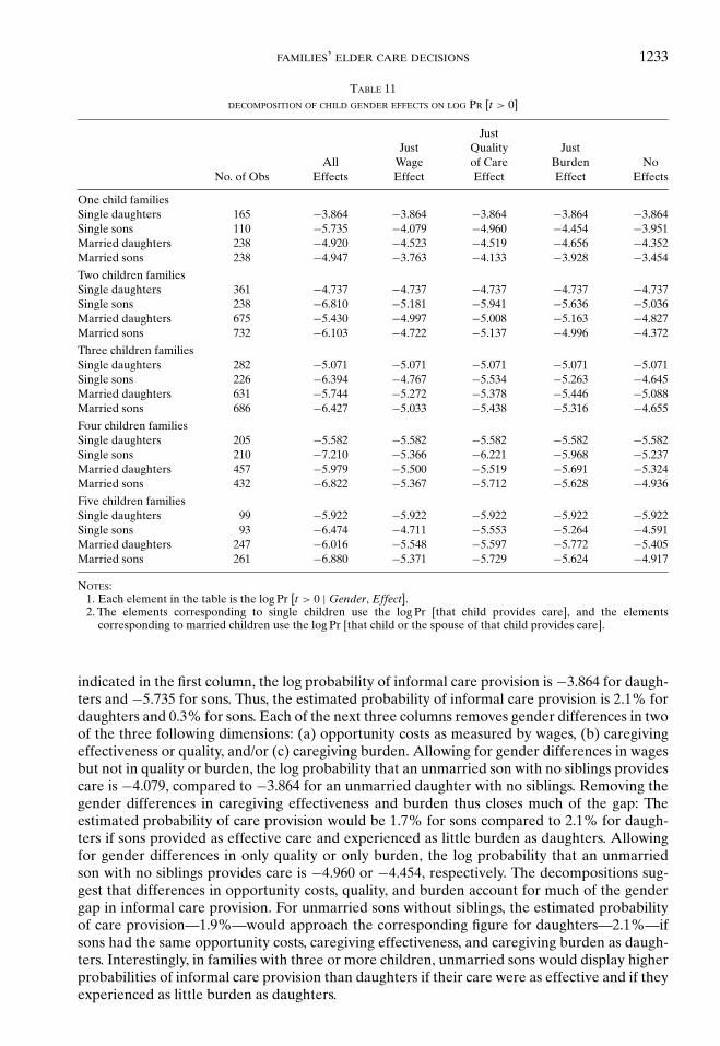
FAMILIES’ ELDER CARE DECISIONS 1233
TABLE 11DECOMPOSITION OF CHILD GENDER EFFECTS ON LOG PR [t > 0]
JustJust Quality Just
All Wage of Care Burden NoNo. of Obs Effects Effect Effect Effect Effects
One child familiesSingle daughters 165 −3.864 −3.864 −3.864 −3.864 −3.864Single sons 110 −5.735 −4.079 −4.960 −4.454 −3.951Married daughters 238 −4.920 −4.523 −4.519 −4.656 −4.352Married sons 238 −4.947 −3.763 −4.133 −3.928 −3.454
Two children familiesSingle daughters 361 −4.737 −4.737 −4.737 −4.737 −4.737Single sons 238 −6.810 −5.181 −5.941 −5.636 −5.036Married daughters 675 −5.430 −4.997 −5.008 −5.163 −4.827Married sons 732 −6.103 −4.722 −5.137 −4.996 −4.372
Three children familiesSingle daughters 282 −5.071 −5.071 −5.071 −5.071 −5.071Single sons 226 −6.394 −4.767 −5.534 −5.263 −4.645Married daughters 631 −5.744 −5.272 −5.378 −5.446 −5.088Married sons 686 −6.427 −5.033 −5.438 −5.316 −4.655
Four children familiesSingle daughters 205 −5.582 −5.582 −5.582 −5.582 −5.582Single sons 210 −7.210 −5.366 −6.221 −5.968 −5.237Married daughters 457 −5.979 −5.500 −5.519 −5.691 −5.324Married sons 432 −6.822 −5.367 −5.712 −5.628 −4.936
Five children familiesSingle daughters 99 −5.922 −5.922 −5.922 −5.922 −5.922Single sons 93 −6.474 −4.711 −5.553 −5.264 −4.591Married daughters 247 −6.016 −5.548 −5.597 −5.772 −5.405Married sons 261 −6.880 −5.371 −5.729 −5.624 −4.917
NOTES:1. Each element in the table is the log Pr [t > 0 | Gender, Effect].2. The elements corresponding to single children use the log Pr [that child provides care], and the elements
corresponding to married children use the log Pr [that child or the spouse of that child provides care].
indicated in the first column, the log probability of informal care provision is −3.864 for daugh-ters and −5.735 for sons. Thus, the estimated probability of informal care provision is 2.1% fordaughters and 0.3% for sons. Each of the next three columns removes gender differences in twoof the three following dimensions: (a) opportunity costs as measured by wages, (b) caregivingeffectiveness or quality, and/or (c) caregiving burden. Allowing for gender differences in wagesbut not in quality or burden, the log probability that an unmarried son with no siblings providescare is −4.079, compared to −3.864 for an unmarried daughter with no siblings. Removing thegender differences in caregiving effectiveness and burden thus closes much of the gap: Theestimated probability of care provision would be 1.7% for sons compared to 2.1% for daugh-ters if sons provided as effective care and experienced as little burden as daughters. Allowingfor gender differences in only quality or only burden, the log probability that an unmarriedson with no siblings provides care is −4.960 or −4.454, respectively. The decompositions sug-gest that differences in opportunity costs, quality, and burden account for much of the gendergap in informal care provision. For unmarried sons without siblings, the estimated probabilityof care provision—1.9%—would approach the corresponding figure for daughters—2.1%—ifsons had the same opportunity costs, caregiving effectiveness, and caregiving burden as daugh-ters. Interestingly, in families with three or more children, unmarried sons would display higherprobabilities of informal care provision than daughters if their care were as effective and if theyexperienced as little burden as daughters.
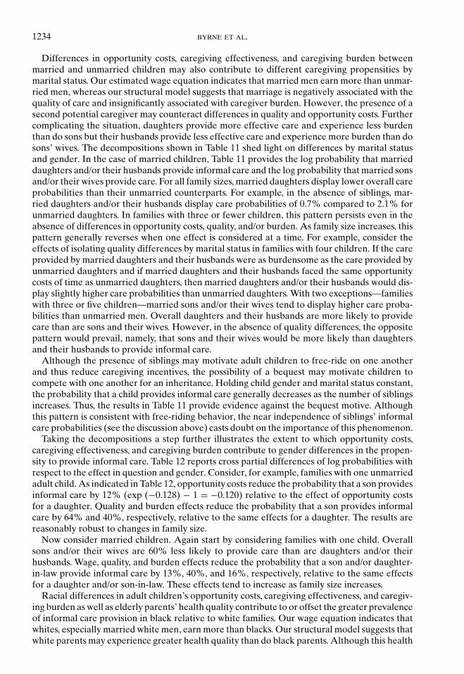
1234 BYRNE ET AL.
Differences in opportunity costs, caregiving effectiveness, and caregiving burden betweenmarried and unmarried children may also contribute to different caregiving propensities bymarital status. Our estimated wage equation indicates that married men earn more than unmar-ried men, whereas our structural model suggests that marriage is negatively associated with thequality of care and insignificantly associated with caregiver burden. However, the presence of asecond potential caregiver may counteract differences in quality and opportunity costs. Furthercomplicating the situation, daughters provide more effective care and experience less burdenthan do sons but their husbands provide less effective care and experience more burden than dosons’ wives. The decompositions shown in Table 11 shed light on differences by marital statusand gender. In the case of married children, Table 11 provides the log probability that marrieddaughters and/or their husbands provide informal care and the log probability that married sonsand/or their wives provide care. For all family sizes, married daughters display lower overall careprobabilities than their unmarried counterparts. For example, in the absence of siblings, mar-ried daughters and/or their husbands display care probabilities of 0.7% compared to 2.1% forunmarried daughters. In families with three or fewer children, this pattern persists even in theabsence of differences in opportunity costs, quality, and/or burden. As family size increases, thispattern generally reverses when one effect is considered at a time. For example, consider theeffects of isolating quality differences by marital status in families with four children. If the careprovided by married daughters and their husbands were as burdensome as the care provided byunmarried daughters and if married daughters and their husbands faced the same opportunitycosts of time as unmarried daughters, then married daughters and/or their husbands would dis-play slightly higher care probabilities than unmarried daughters. With two exceptions—familieswith three or five children—married sons and/or their wives tend to display higher care proba-bilities than unmarried men. Overall daughters and their husbands are more likely to providecare than are sons and their wives. However, in the absence of quality differences, the oppositepattern would prevail, namely, that sons and their wives would be more likely than daughtersand their husbands to provide informal care.
Although the presence of siblings may motivate adult children to free-ride on one anotherand thus reduce caregiving incentives, the possibility of a bequest may motivate children tocompete with one another for an inheritance. Holding child gender and marital status constant,the probability that a child provides informal care generally decreases as the number of siblingsincreases. Thus, the results in Table 11 provide evidence against the bequest motive. Althoughthis pattern is consistent with free-riding behavior, the near independence of siblings’ informalcare probabilities (see the discussion above) casts doubt on the importance of this phenomenon.
Taking the decompositions a step further illustrates the extent to which opportunity costs,caregiving effectiveness, and caregiving burden contribute to gender differences in the propen-sity to provide informal care. Table 12 reports cross partial differences of log probabilities withrespect to the effect in question and gender. Consider, for example, families with one unmarriedadult child. As indicated in Table 12, opportunity costs reduce the probability that a son providesinformal care by 12% (exp (−0.128) − 1 = −0.120) relative to the effect of opportunity costsfor a daughter. Quality and burden effects reduce the probability that a son provides informalcare by 64% and 40%, respectively, relative to the same effects for a daughter. The results arereasonably robust to changes in family size.
Now consider married children. Again start by considering families with one child. Overallsons and/or their wives are 60% less likely to provide care than are daughters and/or theirhusbands. Wage, quality, and burden effects reduce the probability that a son and/or daughter-in-law provide informal care by 13%, 40%, and 16%, respectively, relative to the same effectsfor a daughter and/or son-in-law. These effects tend to increase as family size increases.
Racial differences in adult children’s opportunity costs, caregiving effectiveness, and caregiv-ing burden as well as elderly parents’ health quality contribute to or offset the greater prevalenceof informal care provision in black relative to white families. Our wage equation indicates thatwhites, especially married white men, earn more than blacks. Our structural model suggests thatwhite parents may experience greater health quality than do black parents. Although this health
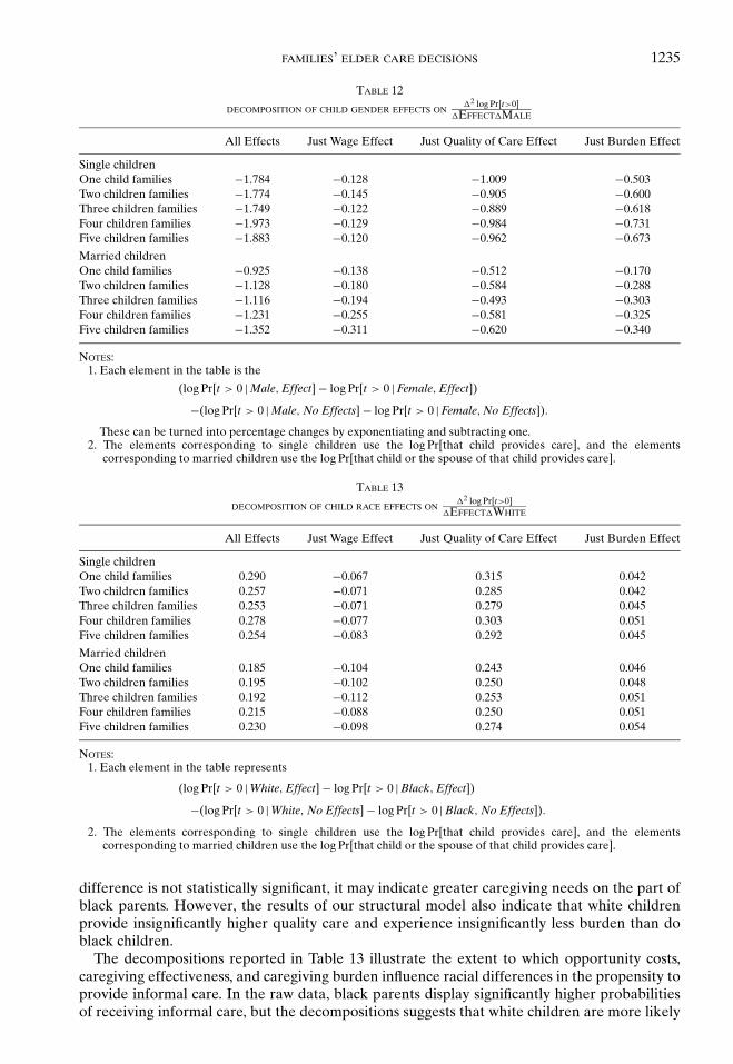
FAMILIES’ ELDER CARE DECISIONS 1235
TABLE 12
DECOMPOSITION OF CHILD GENDER EFFECTS ON�2 log Pr[t>0]
�EFFECT�MALE
All Effects Just Wage Effect Just Quality of Care Effect Just Burden Effect
Single childrenOne child families −1.784 −0.128 −1.009 −0.503Two children families −1.774 −0.145 −0.905 −0.600Three children families −1.749 −0.122 −0.889 −0.618Four children families −1.973 −0.129 −0.984 −0.731Five children families −1.883 −0.120 −0.962 −0.673
Married childrenOne child families −0.925 −0.138 −0.512 −0.170Two children families −1.128 −0.180 −0.584 −0.288Three children families −1.116 −0.194 −0.493 −0.303Four children families −1.231 −0.255 −0.581 −0.325Five children families −1.352 −0.311 −0.620 −0.340
NOTES:1. Each element in the table is the
(log Pr[t > 0 | Male, Effect] − log Pr[t > 0 | Female, Effect])
−(log Pr[t > 0 | Male, No Effects] − log Pr[t > 0 | Female, No Effects]).
These can be turned into percentage changes by exponentiating and subtracting one.2. The elements corresponding to single children use the log Pr[that child provides care], and the elements
corresponding to married children use the log Pr[that child or the spouse of that child provides care].
TABLE 13
DECOMPOSITION OF CHILD RACE EFFECTS ON�2 log Pr[t>0]
�EFFECT�WHITE
All Effects Just Wage Effect Just Quality of Care Effect Just Burden Effect
Single childrenOne child families 0.290 −0.067 0.315 0.042Two children families 0.257 −0.071 0.285 0.042Three children families 0.253 −0.071 0.279 0.045Four children families 0.278 −0.077 0.303 0.051Five children families 0.254 −0.083 0.292 0.045
Married childrenOne child families 0.185 −0.104 0.243 0.046Two children families 0.195 −0.102 0.250 0.048Three children families 0.192 −0.112 0.253 0.051Four children families 0.215 −0.088 0.250 0.051Five children families 0.230 −0.098 0.274 0.054
NOTES:1. Each element in the table represents
(log Pr[t > 0 | White, Effect] − log Pr[t > 0 | Black, Effect])
−(log Pr[t > 0 | White, No Effects] − log Pr[t > 0 | Black, No Effects]).
2. The elements corresponding to single children use the log Pr[that child provides care], and the elementscorresponding to married children use the log Pr[that child or the spouse of that child provides care].
difference is not statistically significant, it may indicate greater caregiving needs on the part ofblack parents. However, the results of our structural model also indicate that white childrenprovide insignificantly higher quality care and experience insignificantly less burden than doblack children.
The decompositions reported in Table 13 illustrate the extent to which opportunity costs,caregiving effectiveness, and caregiving burden influence racial differences in the propensity toprovide informal care. In the raw data, black parents display significantly higher probabilitiesof receiving informal care, but the decompositions suggests that white children are more likely
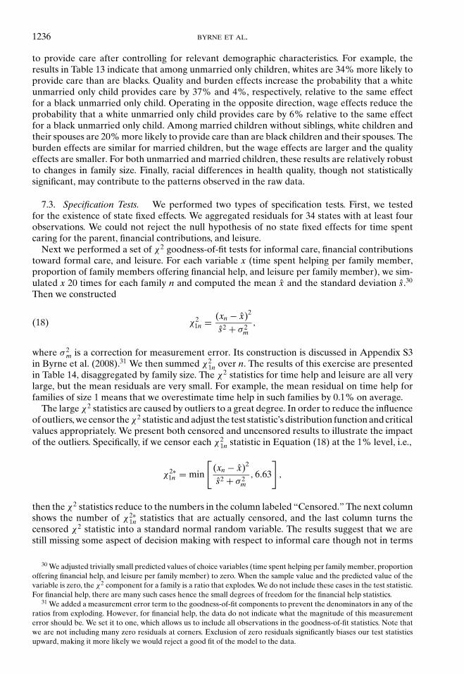
1236 BYRNE ET AL.
to provide care after controlling for relevant demographic characteristics. For example, theresults in Table 13 indicate that among unmarried only children, whites are 34% more likely toprovide care than are blacks. Quality and burden effects increase the probability that a whiteunmarried only child provides care by 37% and 4%, respectively, relative to the same effectfor a black unmarried only child. Operating in the opposite direction, wage effects reduce theprobability that a white unmarried only child provides care by 6% relative to the same effectfor a black unmarried only child. Among married children without siblings, white children andtheir spouses are 20% more likely to provide care than are black children and their spouses. Theburden effects are similar for married children, but the wage effects are larger and the qualityeffects are smaller. For both unmarried and married children, these results are relatively robustto changes in family size. Finally, racial differences in health quality, though not statisticallysignificant, may contribute to the patterns observed in the raw data.
7.3. Specification Tests. We performed two types of specification tests. First, we testedfor the existence of state fixed effects. We aggregated residuals for 34 states with at least fourobservations. We could not reject the null hypothesis of no state fixed effects for time spentcaring for the parent, financial contributions, and leisure.
Next we performed a set of χ2 goodness-of-fit tests for informal care, financial contributionstoward formal care, and leisure. For each variable x (time spent helping per family member,proportion of family members offering financial help, and leisure per family member), we sim-ulated x 20 times for each family n and computed the mean x and the standard deviation s.30
Then we constructed
χ21n = (xn − x)2
s2 + σ 2m
,(18)
where σ 2m is a correction for measurement error. Its construction is discussed in Appendix S3
in Byrne et al. (2008).31 We then summed χ21n over n. The results of this exercise are presented
in Table 14, disaggregated by family size. The χ2 statistics for time help and leisure are all verylarge, but the mean residuals are very small. For example, the mean residual on time help forfamilies of size 1 means that we overestimate time help in such families by 0.1% on average.
The large χ2 statistics are caused by outliers to a great degree. In order to reduce the influenceof outliers, we censor the χ2 statistic and adjust the test statistic’s distribution function and criticalvalues appropriately. We present both censored and uncensored results to illustrate the impactof the outliers. Specifically, if we censor each χ2
1n statistic in Equation (18) at the 1% level, i.e.,
χ2∗1n = min
[(xn − x)2
s2 + σ 2m
, 6.63
],
then the χ2 statistics reduce to the numbers in the column labeled “Censored.” The next columnshows the number of χ2∗
1n statistics that are actually censored, and the last column turns thecensored χ2 statistic into a standard normal random variable. The results suggest that we arestill missing some aspect of decision making with respect to informal care though not in terms
30 We adjusted trivially small predicted values of choice variables (time spent helping per family member, proportionoffering financial help, and leisure per family member) to zero. When the sample value and the predicted value of thevariable is zero, the χ2 component for a family is a ratio that explodes. We do not include these cases in the test statistic.For financial help, there are many such cases hence the small degrees of freedom for the financial help statistics.
31 We added a measurement error term to the goodness-of-fit components to prevent the denominators in any of theratios from exploding. However, for financial help, the data do not indicate what the magnitude of this measurementerror should be. We set it to one, which allows us to include all observations in the goodness-of-fit statistics. Note thatwe are not including many zero residuals at corners. Exclusion of zero residuals significantly biases our test statisticsupward, making it more likely we would reject a good fit of the model to the data.
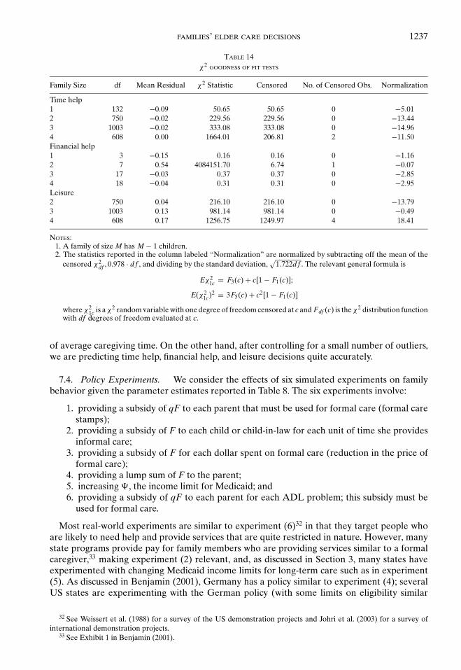
FAMILIES’ ELDER CARE DECISIONS 1237
TABLE 14χ2 GOODNESS OF FIT TESTS
Family Size df Mean Residual χ2 Statistic Censored No. of Censored Obs. Normalization
Time help1 132 −0.09 50.65 50.65 0 −5.012 750 −0.02 229.56 229.56 0 −13.443 1003 −0.02 333.08 333.08 0 −14.964 608 0.00 1664.01 206.81 2 −11.50Financial help1 3 −0.15 0.16 0.16 0 −1.162 7 0.54 4084151.70 6.74 1 −0.073 17 −0.03 0.37 0.37 0 −2.854 18 −0.04 0.31 0.31 0 −2.95Leisure2 750 0.04 216.10 216.10 0 −13.793 1003 0.13 981.14 981.14 0 −0.494 608 0.17 1256.75 1249.97 4 18.41
NOTES:1. A family of size M has M − 1 children.2. The statistics reported in the column labeled “Normalization” are normalized by subtracting off the mean of the
censored χ2df , 0.978 · df , and dividing by the standard deviation,
√1.722df . The relevant general formula is
Eχ21c = F3(c) + c[1 − F1(c)];
E(χ21c)2 = 3F5(c) + c2[1 − F1(c)]
where χ21c is a χ2 random variable with one degree of freedom censored at c and Fdf (c) is the χ2 distribution function
with df degrees of freedom evaluated at c.
of average caregiving time. On the other hand, after controlling for a small number of outliers,we are predicting time help, financial help, and leisure decisions quite accurately.
7.4. Policy Experiments. We consider the effects of six simulated experiments on familybehavior given the parameter estimates reported in Table 8. The six experiments involve:
1. providing a subsidy of qF to each parent that must be used for formal care (formal carestamps);
2. providing a subsidy of F to each child or child-in-law for each unit of time she providesinformal care;
3. providing a subsidy of F for each dollar spent on formal care (reduction in the price offormal care);
4. providing a lump sum of F to the parent;5. increasing �, the income limit for Medicaid; and6. providing a subsidy of qF to each parent for each ADL problem; this subsidy must be
used for formal care.
Most real-world experiments are similar to experiment (6)32 in that they target people whoare likely to need help and provide services that are quite restricted in nature. However, manystate programs provide pay for family members who are providing services similar to a formalcaregiver,33 making experiment (2) relevant, and, as discussed in Section 3, many states haveexperimented with changing Medicaid income limits for long-term care such as in experiment(5). As discussed in Benjamin (2001), Germany has a policy similar to experiment (4); severalUS states are experimenting with the German policy (with some limits on eligibility similar
32 See Weissert et al. (1988) for a survey of the US demonstration projects and Johri et al. (2003) for a survey ofinternational demonstration projects.
33 See Exhibit 1 in Benjamin (2001).
1238 BYRNE ET AL.
to those in experiment (6)). We have found no examples in the literature providing subsidiessimilar to experiment (3).
Given the small marginal product of formal and informal care on Q implied by the parameterestimates in Table 8, almost all of the policy experiments would have essentially no effect onbehavior. Experiment (1) suggests that formal care stamps would have little impact on expen-ditures for formal care. Most families without formal care expenditures prior to the experimentwould exhaust their formal care stamps but spend no out of pocket funds on formal care. To alarge degree, those with formal care expenditures would replace their own expenditures withprogram expenditures with little effect on the level of formal care or informal care.34
Experiments (2) and (3) essentially reduce the price of informal and formal care. However,because the family resources expended on both are small and both marginal products are small,the effects of the subsidy would be small. Experiment (4) indicates that a lump sum subsidyto the parent would be used to supplement consumption. This is similar to results discussed inBenjamin (2001). Thus, a lump sum subsidy would have very little effect on formal or informalcare or the health (Q) of the parent. Experiments (5) and (6) are small deviations of experiment(1) and would have similar though smaller effects.
Overall, the results of these experiments suggest that variation in state Medicaid policy wouldhave little effect on long-term care decisions. The average policy results are very small becausemost families are at a corner solution and it would take a very expensive policy to move themaway from the corner. For the most part, the proposed policies result in an increase in utilityfor those who were already providing formal and/or informal care and little change in behavioramong everyone else. These results are consistent with results in ES where no significant state ef-fects were found but inconsistent with Cutler and Sheiner (1993) that found small macro effects.We measure the effect of policy changes given that respondents reside in the community and,hence, under some situations, underestimate the effect of changes in policy on community-basedcaregiving. For example, policy changes with regard to Medicaid income limits or subsidies forhome health care may imply different choices for community-based care versus institutionaliza-tion. Institutional care may be a decision under some policy parameters, whereas other policyparameters may induce families to care for the elderly parent at home.
8. CONCLUSIONS
We develop and estimate a game-theoretic model of families’ decisions concerning the provi-sion of informal and formal home health care for elderly individuals. In addition to consumptionand leisure, a family member’s utility depends on the health quality of elderly relatives as wellas her own provision of informal care. Each individual or married couple makes caregivingdecisions conditional on the decisions of the other family members. We use the FOCs of themodel to solve for the errors as relatively simple functions of the parameters and construct thecorresponding likelihood function.
The structure of the model allows us to distinguish among several underlying explanationsfor patterns in care provision. In particular, caregiver burden, caregiving effectiveness, and op-portunity costs vary within and across families. Also, the model allows for both self-interest andaltruism in the sense that family members value their own consumption and leisure as well as thehealth quality of their elderly relatives. Our results suggest that most family members, especiallychildren and children-in-law, consider caregiving burdensome, that informal care, especially careprovided by a spouse, has a small effect on health quality, and that children care about theirparents’ health quality. Thus, the tendency of spouses instead of adult children to provide care isattributable to the lower burden experienced by spouses in the caregiving role instead of differ-ences in care effectiveness between spouses and children or selfishness on the part of children.Apparently, the closer bonds between parents and their own children than between parents andchildren-in-law enhance the quality of care and diminish the burden experienced by members
34 See Pezzin et al. (1996) for similar results.
FAMILIES’ ELDER CARE DECISIONS 1239
of the younger generation. As expected, children with higher opportunity costs of time exhibitlower caregiving probabilities than their siblings or peers. Interestingly, however, we find thatthe greater reliance on formal care among more highly educated elderly individuals is due todifferences in care effectiveness instead of income.
The structure of the model sheds light on the roles of gender, marital status, family size, andrace. Overall, daughters display higher care probabilities than do sons. Our decompositions sug-gest that differences in opportunity costs, quality, and burden account for much of the gendergap in informal care provision. Unmarried daughters display higher overall care probabilitiesthan their married counterparts, regardless of family size. In relatively small families, this pat-tern persists even in the absence of differences in opportunity costs, quality, and/or burden.Overall, daughters and their husbands are more likely to provide care than are sons and theirwives. However, in the absence of quality differences, the opposite pattern would prevail. Racialdifferences in adult children’s opportunity costs and elderly parents’ health quality contributeto the greater prevalence of informal care provision in black relative to white families, offsettingdifferences in quality and burden of care.
Goodness-of-fit tests show that our model fits the data fairly well. In addition, we fail to rejectthe hypothesis that there is no additional variation across states not captured in the model. Thisresult suggests that our simplification of the Medicaid benefit structure performs well.
The structural nature of the estimates enables us to perform policy experiments similar tothose proposed by policymakers. For example, we simulate the provision of a lump sum that canbe spent only on care as well as price subsidies for informal and formal home health care. Asa result of the relative ineffectiveness of both forms of care, we find little effect of these policychanges.
Although our results yield important insights concerning families’ elder care decisions, sev-eral limitations are worth noting. First, the 1993 wave of AHEAD data does not include anynursing home residents. The inclusion of nursing home residents in subsequent waves will enableus to investigate the effects of proposed or actual policies on the use of institutional care. Forexample, subsidies for home health care may induce some families to care for the elderly athome instead of an institution. Second, the survey instrument used in subsequent waves elicitsmore information about caregivers, enabling us to further improve our model. Third, our useof a static model obscures the dynamic aspects of families’ care decisions. The availability ofpanel data will enable us to estimate a dynamic extension of our structural model. Using severalwaves of AHEAD data, future work will explore whether family members specialize accordingto their comparative advantages in market production, caregiving, or other forms of nonmarketproduction or whether siblings take turns providing informal care. If children take turns care-giving, the use of panel data will enable us to examine possible causes of this behavior includingburnout. Finally, our current work does not adequately address differences by race. In futurework, we plan to estimate separate models by race to examine the extent to which characteristicssuch as child gender operate differently by race.
APPENDIX: CONSTRUCTION OF CHILD CARING TIME
A key issue in estimation concerns the interpretation of data on caregiving time t jik. In thesurvey, there are two relevant questions:
1) How many days per week does the helper provide help?2) How many hours per day does the helper provide help on days when she helps?
Although the responses to the second question provide a continuous measure of hours perday, responses to the first question are categorical: (a) every day, (b) several times a week, (c)once per week, (d) less than once per week, and (e) never. We can use the answers to these two
1240 BYRNE ET AL.
questions to construct a “pseudo” continuous variable:
t jik =
7π j ik/168 if she helps every day
3.5π j ik/168 if she helps several times a week
π j ik/168 if she helps once per week
0.5π j ik/168 if she helps less than once per week
0 if she never helps,
(A.1)
where π jik is the answer to the second question.35
Unfortunately, the AHEAD respondents were asked about help from children only if theyhad an ADL or IADL problem. This feature of the survey design may bias the amount ofreported care downwards. However, it is reasonable to assume that parents needing care fromchildren are likely to have an ADL or IADL, and, at the time we constructed our data, therewere no better data available.
REFERENCES
AGUIRREGABIRIA, V., AND P. MIRA, “Sequential Estimation of Dynamic Discrete Games with MultipleEquilibria,” Econometrica 75 (2007), 1–53.
BARBER, C. E., “Burden and Family Care of the Elderly,” in S. J. Bahr and E. T. Peterson, eds., Aging andthe Family (Lexington, MA: Lexington Books, 1989).
BENJAMIN, A., “Consumer-Directed Services at Home: A New Model for Persons with Disabilities,” HealthAffairs 20 (2001), 80–95.
BERNHEIM, D., A. SHLEIFER, AND L. SUMMERS, “The Strategic Bequest Motive,” Journal of Political Economy93 (1985), 1045–76.
BOAZ, R. F., AND J. HU, “Determining the Amount of Help Used by Disabled Elderly Persons at Home:The Role of Coping Resources,” Journals of Gerontology, Series B: Psychological Sciences and SocialSciences 52 (1997), S317-24.
BOERSCH-SUPAN, A., L. KOTLIKOFF, AND J. MORRIS, “The Dynamics of Living Arrangements of the Elderly,”NBER Working Paper 2787, 1988.
BUREAU OF ECONOMIC ANALYSIS, http://www.bea.doc.gov/bea/regional/data.htm, 1999.BUREAU OF LABOR STATISTICS, State Occupational Employment Statistics Survey, http://stats.bls.gov/
oeshome.htm, 1998.BYRNE, D., M. GOEREE, B. HIEDEMANN, AND S. STERN, “Income Eligibility Criteria for Medicaid,”
http://faculty.virginia.edu/stevenstern/resint/ltcstf/medicaideligibility.pdf, 2003.——, ——, ——, AND ——, “Appendices and Supplementary Tables for Formal Home Health Care,
Informal Care, and Family Decision-Making,” http://faculty.virginia.edu/stevenstern/resint/ltcstf/hrssupplement.html, 2008.
CANTOR, M. H., “Strain among Caregivers: A Study of Experience in the United States,” The Gerontologist23 (1983), 597–604.
CENSUS OF POPULATION AND HOUSING, “Earnings by Occupation and Education (SSTF22),”http://govinfo.kerr.orst.edu/earn-stateis.html, 1990.
CHECKOVICH, T., AND S. STERN, “Shared Caregiving Responsibilities of Adult Siblings with Elderly Parents,”Journal of Human Resources 37 (2002), 441–78.
CONGRESSIONAL RESEARCH SERVICE: SUBCOMMITTEE ON HEALTH AND THE ENVIRONMENT, Medicaid SourceBook: Background Data and Analysis. (Washington, DC: U.S. Government Printing Office, 1993).
COUCH, K. A., M. C. DALY, AND D. A. WOLF, “Time? Money? Both? The Allocation of Resources to OlderParents,” Demography 36 (1999), 219–32.
CUTLER, D., AND L. SHEINER, “Policy Options for Long-Term Care,” NBER Working Paper 4302, 1993.DIWAN, S., C. BERGER, AND E. MANNS, “Composition of the Home Care Service Package: Predictors of
Type, Volume, and Mix of Services Provided to Poor and Frail Older People,” The Gerontologist 37(1997), 169–81.
35 Alternatively, we could have set up bracketed amounts that are truer to the nature of the first question. Usingthe brackets is much harder, and it adds precision only for two of the five categories. These two occur for 949 helpersout of a total of 3,144 helpers (30.1%). Stern (1994) shows that the added precision gained by treating the variable asbracketed is very small in a similar problem.
FAMILIES’ ELDER CARE DECISIONS 1241
ENGERS, M., AND S. STERN, “Long-Term Care and Family Bargaining,” International Economic Review 43(2002), 73–114.
ETTNER, S. L., “The Opportunity Costs of Elder Care,” Journal of Human Resources 31 (1996), 189–205.FRANKFATHER, D., M. J. SMITH, AND F. G. CARO, Family Care of the Elderly: Public Initiatives and Private
Obligations (Lexington, MA: Lexington Books, 1981).GOURIEROUX, C., A. MONFORT, E. RENAULT, AND A. TROGNON, “Generalized Residuals,” Journal of Econo-
metrics 34 (1987), 5–32.HAJIVASSILIOU, V., D. MCFADDEN, AND P. RUUD, “Simulation of Multivariate Normal Rectangle Probabilities
and Their Derivatives: Theoretical and Computational Results,” Discussion Paper No. 1021R, CowlesFoundation, Yale University, 1994.
HAUSMAN, J., “The Econometrics of Nonlinear Budget Sets,” Econometrica 53 (1985), 1255–82.HIEDEMANN, B., AND S. STERN, “Strategic Play among Family Members When Making Long-Term Care
Decisions,” Journal of Economic Behavior and Organization 40 (1999), 29–57.HOERGER, T. J., G. A. PICONE, AND F. A. SLOAN, “Public Subsidies, Private Provision of Care and Living
Arrangements of the Elderly,” Review of Economics and Statistics 78 (1996), 428–40.HOROWITZ, A., “Family Caregiving to the Frail Elderly,” Annual Review of Gerontology and Geriatrics 6
(1985), 194–246.JOHNSON, C. L., “Dyadic Family Relations and Social Support,” The Gerontologist 23 (1983), 377–83.——, AND D. J. CATALANO, “Childless Elderly and Their Family Supports,” The Gerontologist 21 (1981),
612–18.JOHRI, M., F. BELAND, AND H. BERGMAN, “International Experiments in Integrated Care for the Elderly: A
Synthesis of the Evidence,” International Journal of Geriatric Psychiatry 18 (2003), 222–35.KOTLIKOFF, L. J., AND J. N. MORRIS, “Why Don’t the Elderly Live with Their Children? A New Look,” in
D. A. Wise, ed., Issues in the Economics of Aging (Chicago: University of Chicago Press, 1990).LEE, G., J. DWYER, AND R. COWARD, “Residential Location and Proximity to Children Among Impaired
Elderly Parents,” Rural Sociology 55 (1990), 579–89.MACK, K., AND L. THOMPSON, “A Decade of Informal Caregiving: Are Today’s Informal Caregivers Different
than Informal Caregivers a Decade Ago?” Data Profile (Washington, DC: Center on an Aging Society,2004), http://www.aging-society.org.
MACKEN, C., “A Profile of Functionally Impaired Elderly Persons Living in the Community,” Health CareFinancing Review 7 (1986), 33–50.
MANTON, K., AND X. L. GU, “Changes in the Prevalence of Chronic Disability in the United States Blackand Nonblack Population above Age 65 from 1982 to 1999,” Proceedings of the National Academy ofSciences of the United States of America 98 (2001), 6354–59.
MATTHEWS, S. H., AND T. T. ROSNER, “Shared Filial Responsibility: The Family as the Primary Caregiver,”Journal of Marriage and the Family 50 (1988), 185–95.
MCGARRY, K., “Inter Vivos Transfers and Intended Bequests,” Journal of Public Economics 73 (1999),321–51.
MILLER, B., AND A. MONTGOMERY, “Family Caregivers and Limitations in Social Activities,” Research onAging 12 (1990), 72–93.
NATIONAL CENTER FOR HEALTH STATISTICS, Health, United States, 1995 (Hyattsville, MD, 1996).NORGARD, T., AND W. RODGERS, “Patterns of In-Home Care Among Elderly Black and White Americans,”
Journals of Gerontology, Series B: Psychological Sciences and Social Sciences 52 (1997), 93–101.NORTON, E., AND C. VAN HOUTVEN, “Intervivos Transfers and Exchange,” Southern Economic Journal 73
(2006), 157–72.PEZZIN, L., P. KEMPER, AND J. RESCHOVSKY, “Does Publicly Provided Home Care Substitute for Family
Care? Experimental Evidence with Endogenous Living Arrangements,” Journal of Human Resources31 (1996), 650–76.
PEZZIN, L. E., AND B. S. SCHONE, “The Allocation of Resources in Intergenerational Households: AdultChildren and Their Elderly Parents,” American Economic Review 87 (1997), 460–64.
——, AND ——, “Intergenerational Household Formation, Female Labor Supply and Informal Caregiving:A Bargaining Approach,” Journal of Human Resources 34 (1999), 475–503.
SCHOONOVER, C. B., E. M. BRODY, C. HOFFMAN, AND M. H. KLEBAN, “Parent Care and GeographicallyDistant Children,” Research on Aging 10 (1988), 472–92.
SLOAN, F. A., G. PICONE, AND T. J. HOERGER, “The Supply of Children’s Time To Disabled Elderly Parents,”Economic Inquiry 35 (1997): 295–308.
SPEAR, A., AND R. AVERY, “Who Helps Whom in Older Parent-Child Families,” Journal of Gerontology 48(1993), S64–S73.
SPECTOR, W. D., J. A. FLEISHMAN, L. E. PEZZIN, AND B. C. SPILLMAN, “The Characteristics of Long-TermCare Users,” in G. S. Wunderlich and P. O. Kohler, eds., Improving the Quality of Long-Term Care(Washington, DC: National Academies Press, 2001).
STERN, S., “Two Dynamic Discrete Choice Estimation Problems and Simulation Method Solutions,” Reviewof Economics and Statistics 76 (1994), 695–702.
1242 BYRNE ET AL.
——, “Estimating Family Long-Term Care Decisions in the Presence of Endogenous Child Characteristics,”The Journal of Human Resources 30 (1995), 551–80.
STOLLER, E. P., AND L. L. EARL, “Help with the Activities of Everyday Life: Sources of Support for theNon-Institutionalized Elderly,” The Gerontologist 23 (1983), 64–70.
U.S. CENSUS BUREAU, “U.S. Interim Projections by Age, Sex, Race, and Hispanic Origin,” Table 2a.http://www.census.gov/ipc/www/usinterimproj/, 2004.
U.S. DEPARTMENT OF HEALTH AND HUMAN SERVICES, HEALTH CARE FINANCING ADMINISTRATION, State ProfileData System: Characteristics of Medicaid State Programs, Volume 1. (Washington, DC, 1992).
——, 2000 National Health Expenditures. http://www.hcfa.gov/stats/NHE-OAct/, 2000.WEISSERT, W., C. CREADY, AND J. PAWELAK, “The Past and Future of Home- and Community-Based Long-
Term Care,” The Milbank Quarterly 66 (1988), 309–88.WHITE-MEANS, S. I., “The Demands of Persons with Disabilities for Home Health Care and the Economic
Consequences for Informal Caregivers,” Social Science Quarterly 78 (1997), 955–72.WOLF, D., “Kin Availability and the Living Arrangements of Older Women,” Social Science Research 13
(1984), 72–89.——, AND B. SOLDO, “Household Composition Choices of Older Unmarried Women,” Demography 25
(1988), 387–403.