Form factors for deformed spheroids in stokes flow

Form Factors for Deformed Spheroids in Stokes Flow

VIVIAN OBRIEN The Johns Hopkins University, Silver Spring, Maryland

Closed analytic Stokes flow solutions for general shapes are quite improbable, but semi- analytic numerical procedures allow flow calculations for a variety of shapes. The change in drag with change in shape from a sphere, here expressed in terms of a form factor, is discussed and compared to empirical shape factors developed from sedimentation experiments.

Stokes flow describes the slow motions of small particles, for instance macromolecules in biological systems, fallout from an atomic blast or silt in a river. Theory for a sphere is well-known, but real life particles are seldom spherical. A semi-analytical computer program has been developed for steady uniform flow past a wide variety of deformed spheroids (1). The results can be applied im- mediately to sedimentation problems, and, with that in view, the form factor for Stokes drag is investigated and compared to conventional shape factors.

ANALYSIS

Table 1 is the background for the calculation. Assume slow steady simple axisymmetric flow of incompressible fluid and the equations of motion reduce to Stokes stream function equation ( 2 ) . The equation and its general solution ( 3 ) have been known a long time. The form of solution was given by Savic ( 4 ) where the function is a Gegenbauer polynomial of order n and index (- $ ) . Apply the general solution to the problem of uniform flow past deformed spheroids. At to the solution is required to approach (r)2/2 sin2 8, the uniform flow term. Coeffi-

cients for powers of r greater than two are zero. Viscous nonslip at the body boundary requires ur = ve = 0. The existence of the unique solution for an arbitrary closed body of revolution can be proved, but it would require an infinity of terms, in general. For the semiandytical calculations a finite number of terms is taken as a com- promise. The coefficients of + are computed by matching boundary conditions at a finite number of points of the body contour. The contour is given here in the normal- ized form of unit circle plus a deformation, Figure 1. The deformation need not be small but as the magnitude of the deformation approaches zero, results should reduce to the recent analyses for slightly distorted spheroids (5, 6).

Table 2 shows the steps in the calculation scheme. Given a deformed contour, m values of 8 are chosen. The input is either T (8) read in from a polar plot or r calculated by a formula. The velocity boundary conditions lead to a set of simultaneous equations for the coefficients, a matrix in the machine. Each stagnation point contrib- utes one equation to the set, 2m + 2 equations in all, The equation set is solved by an iterative matrix inversion, yielding the coefficients. By using the values of the coeffi-

TABLE 1. EQUATIONS AND BOUNDARY CONDITIONS

Steady Stokes flow equation in a2 1 - p2 a 2 spherical polar coordinates (2 ) -+--) r2 ap2 !#=o $ = stream function

General solution ( 3 , 4 )

Boundary conditions

,u = cos 6 W

lii = S Cn-'/z ( p ) (unrn + bnra+2 + cnr-n+1 + dnr-*+3) C,-% ( p ) = Gegenbauer polynomial n=2

1. Uniform flow at infinity

Page 870

2. Zero velocity at rigid body surface 1 a$ u7 = -- = 0 rz a@

body

November, 1968

8 5 .90 .95

Deformed Spheroid I I + ~ ( e ) Fig. 1. Contour of a porticle.

cients, +, is calculated for the body points used in the computation. The stream function should be zero, but, of course, is not exactly so for the approximate solution. The accuracy is given by the order of $. The $ value is also checked at intermediate body points not used in calculation. Values of stream function, velocity and vorticity can be computed at field points, usually several hundred. The output gives all information necessary to plot the complete flow field. The dimensional drag value is given simply by the coefficient bz multiplied by (4 TT 7 a U ) (1 ) . (Here 7) = fluid viscosity, a = equatorial radius, U = velocity).

The only grossly deformed spheroids for which complete analytic results are known are ellipsoids (7, 8). Fig- ure 2 shows a comparison of drag values from the computer program and exact analytic ones. The drag ratio d is drag of the deformed body divided by drag of the sphere 6 w 7) a U. The deviations between the approximate values and the exact ones are the order of magnitude of

TABLE 2. COMPUTER PROGRAM

INPUT a. Read in r( ej ) , 0 < j 4 m

b. Calculater(B,) = 1 + f € k p k K

k = l

2( m + 1) simultaneous linear equations MATRIX (r

Solve for 2m + 2 coefficients in j i I I I I

SOLVE

CHECK Is + = 0 at ej; other e on body?

COMPUTE Compute $( r , e), velocity and/or vorticity

Read out information OUTPUT

0 Calculated (m=10)

Prolate Ellipsoids

1.05 1.10 L.15 1.20

Drag Ratio, d

Fig. 2. Drag ratios for ellipsoids.

the + check, confirming the computed accuracy. As can be seen, the calculations with m = 10 do not give accept- able results, $ - 0 (10.3, for oblate ellipsoids of high eccentricity. For these very deformed spheres the series converges slowly and not enough terms have been kept for a good approximation. Actually the use of a spherical solution is not quite appropriate; better results could be expected if a spheroidal series solution were used instead (1). All results reported here are for m = 10 (22 x 23 matrix) using only single precision arithmetic and spherical polar solutions.' For an m this size a single body case averages about 0.001 hr. of machine time on the IBM 7094. The $ checks were O(lO-3) for almost all the bodies shown. Spheroidal solutions [Appendix I (1 ) ] require hypergeometric series with imaginary arguments and thus complex arithmetic inversion routines. When these are programmed double precision arithmetic should also be included. Questions of optimum programming, accuracy, etc. for grossly deformed spheroids awaits numerical experiments using improved programs.

Now consider new bodies for which no analytic soh- tions are known. Figure 3 shows a class of bodies formed when deformations are proportional to cos2 e or @-square deformations. The bodies resemble the prolate and oblate ellipsoids inscribed. Here E is the axial deformation, the amount of squeezing or stretching the sphere. The drag

1- i-7 t -t-7 r-11

I - --_^I -2 2 6

161, Deformation Parameter

Fig. 3. Bodies with p-square deformations.

Tabular material has been deposited as document NAPS-00106 with the American Documentation Institute, Photoduplication Service, Library of Congress, Washington, 25, D.C and may be obtained for $3.00 for photoprints or $1.00 for 35-mm. n&xofilrn.

Vol. 14, No. 6 AlChE Journal Page 871

magnitude of deformotion, E

Fig. 4. Drag ratios for bodies with even p-square deformations.

d

1.06

ratio of these bodies is shown in Figure 4 as a function of t. The drag ratio predicted on the basis of Brenner’s linear perturbation analysis ( 5 ) is also shown. The ratios should agree near E = 0 and they do. Since the undeformed sphere has unit drag ratio, the drag ratio minus 1 can be considered the drag change due to the deformation. Call it form factor f ; this shows there is a positive f for deformed spheroids larger than the unit sphere, nega- tive f for bodies smaller than the sphere.

The drag curve in Figure 4 is for symmetrical p-square deformations, front and back deformed equally. The program can handle deformations without this symmetry. A number of cases were run with e l , denoting front hemisphere deformation, e2 the back. Table 3 shows the chart of form factor, f , calculated for the various p2 deformations. The values on the diagonal where €1 = €2 were shown on the previous figure. Antisymmetrical deformations, €1 = - €2, give values on the opposite diagonal. Form factors f for bodies with only one hemisphere deformed lie within the cross. Figure 5 illustrates the drag curves and the corresponding linear perturbation lines.

Figure 6 shows more body classes considered in the

.

E2 -0.5

+ 0.5 0.047 +0.4 0.027 +0.3 0.009 +0.2 -0.007 +0.1 -0.020

0 -0.031 -0.1 -0.041 -0.2 -0.048 -0.3 -0.054 -0.4 -0.057 -0.5 -0.059

f

06

-.02

.I .2 .3 .4 C

Fig. 5. Drag ratios for bodies with various p-square deformations.

Spheroids with p (cos 0 ) deformations

Fig. 6. Other deformed spheroids used in program.

TABLE 3. FORM FACTORS FOR MU-SQUARE DEFORMATION, f (p2: €1, c 2 )

€1 -0.4 -0.3 -0.2 -0.1 0 +0.1 +0.2

0.050 0.031 0.013

-0.003 -0.016 -0.027 -0.037 -0.044

-0.054 -0.050

-0.057

0.054 0.059 0.035 0.040 0.018 0.023 0.002 0.008

-0.011 -0.005 -0.022 -0.016 -0.032 -0.025 -0.039 -0.033 -0.045 -0.039 -0.050 -0.044 -0.054 -0.048

0.066 0.047 0.030 0.015 0.002

-0.009 -0.018 -0.025 -0.032 -0.037 ,-0.041

0.075 0.056 0.039 0.024 0.011 0

-0.009 -0.016 4 . 0 2 2 -0.027 -0.031

0.086 0.067 0.050 0.035 0.022 0.011 0.002

-0.005 -0.011 -0.016 -0.020

0.098 0.079 0.063 0.048 0.035 0.024 0.015 0.008 0.002

-0.003 -0.007

+0.3

0.111 0.093 0.077 0.063 0.050 0.039 0.030 0.023 0.018 0.013 0.009

+0.4 +0.5

0.127 0.145 0.109 0.127 0.093 0.111 0.079 0.098 0.067 0.086 0.056 0.075 0.047 0.066 0.040 0.059 0.035 0.054 0.031 0.050 0.027 0.047

(last figure may be in error near edges of chart)

Page 872 AlChE Journal November, 1968

i 8 I I -4 -.3 -.2 -.I 0 .I .2 .3 4 . 5

c

Fig. 7. Drag ratios for bodies with p deformations.

program. At the top are cos 0 (or p) deformations. The center is a limacon; the term hemi-limacon has been coined for the side shapes. Deformed bodies below cor- respond to various deformations in p , quite a variety of shapes. Figure 7 shows drag ratios for p deformations, and also the linear perturbation lines which agree for small deformations. Complete results are available for every body represented by a point on the drag curves. A way of illustrating the results for a single body is the streamline plot as shown in Figure 8. The streamlines of the sphere are shown for comparison.

goo

9 = 0.062, 0.125, 0 . 2 5 0.50

Fig. 8. Streamlines for a deformed spheroidal body.

Conceptually the program could be run for completely arbitrary bodies of revolution, read in directly from a polar plot, for instance. However, with the present program there was loss of accuracy with grossly deformed spheroids, body contour,s with discontinuities in slope, and contours that were locally concave. Accuracy could be improved somewhat by taking more points and by judici- ous choice of 6 values. Yet very accurate results were limited mostly to smooth convex bodies with deformations up to (say) 30% of the undeformed radius, thus elimi- nating many bodies of interest. Modification of the program to ensure the most accurate evaluation of matrix elements and writing the program in terms of the general spheroidal solutions could enlarge the scope considerably. Even the limitation to axisymmetric bodies can be re- moved and a similar technique used with the three- dimensional solution of Acrivos and Taylor ( 6 ) . Exten- sion to include the first-order effect in Reynolds number was shown in principle several years ago (9).

SHAPE FACTORS

How do the results relate to the conventional way of looking at nonspherical particles in sedimentary flow? The drag ratio d shown here is just the shape factor considered by Fuchs ( l o ) , or Happel and Brenner (11). Thus the present computer program allows direct evaluation of the shape factor for moderately deformed spheroids. Improvements to the program would allow inclu- sion of more grossly deformed particles.

I t is often easy to compute the drag ratio, but is it possible that there is a simpler geometric way to predict rl for deformed spheroids? Consider a deformed body with an inscribed sphere and a circumscribed sphere. By a theorem of Hill and Power (12), the Stokes drag of the body is bounded above by the Stokes drag of the outer sphere, from below by the inner sphere drag. The geometric factors with the same bounds relative to inscribed and circumscrfbed spheres are volume and cross- sectional area (not perimeter, or surface area).

Long ago attempts were made to estimate the drag of a nonspherical particle with the drag of a sphere with equal volume, sometimes called the equivalent sphere. This was not too successful, as shown by experiments (13, 1 4 ) and the comparison with ellipsoid theory in Figure 9. The drag curve for the equivalent spheres lies within the upper and lower bounds determined by the circumscribed and inscribed spheres, but it does not follow the ellipsoid drag curve very well. Efforts have been made to include empirical sphericity factors (related to the surface area of the particle), circularity factors (related to the projected area normal to the direction

I / l----- I /

- 5 - 4 - 3 - 2 - 1 0 I 2 3 4 5 6 c , axial deformation

Fig. 9. Drag curve for equivalent spheres vs exact analytic drag curve for ellipsoids.


, 1 \ \ I ,I 2 2o Body Contour Within Circle Body Contour Outride Circle

I5

Ellipse (exact)

. * Ellipsoids (exact) - 0 Various Y' deformations

m Pear shape

0 "Super circle"

05

10 Upper Bound Lover Bound

Fig. 10. Correlation of form foctor f with change in cross-sectional area.

of motion), and so on to get a better fit with experimental data (14) . They have no theoretical basis.

The numerical analyses furnish information to inspect geometric factors upon a firm basis. Direct attention to rl - 1 = f , the form factor, showing the change in drag ratio due to the change in shape. Cross-sectional area can be correlated with form factor f for these axisymmetric bodies. That is, there is good correlation of f with a change in cross-sectional area due to the change in shape, Figure 10. If the deformed body is wholly within the undeformed sphere, or wholly without, the difference in area between the body contour and the unit circle can be related approximately by f = 0.b- ' AA, AA being the change in area. The figure shows the results for a large number of bodies whose drag (and thereby f ) were calculated by the computer program. Note the correlation is almost perfect for true ellipsoids. I t is fairly good for bodies that resemble ellipsoids of small eccentricity but poorer for larger, nonellipsoidal deformations. The worst correlation occurs for three super-circle contours with height equal to diameter, bodies with deformations y(p2 - p4) that do not resemble ellipsoids at all. [For y = 0.285 the cross section can hardly be distinguished from Hein's super-circle defined in Cartesian coordinates as x5/2 f $I2 = 1, (H)]. Even if the body is not wholly without the undeformed sphere, the form factor correlation with area change is not unreasonable, as shown by the pear-shape bodies (deformation proportional to p + f ) . However, the correlation is not good enough for prediction purposes.

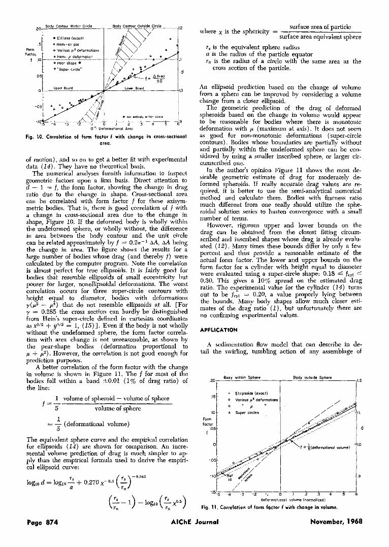
A better correlation of the form factor with the change in volume is shown in Figure 11. The f for most of the bodies fall within a band 20.01 (1% of drag ratio) of the line:

1 volume of spheroid - volume of sphere f = -

5 volume of sphere

1 _ - - (deformational volume) 5

The equivalent sphere curve and the empirical correlation for ellipsoids (14 ) are shown for comparison, An incre- mental volume prediction of drag is much simpler to apply than the empirical formula used to derive the empirical ellipsoid curve:

-0.345 f S

a loglo d = loglo - + 0.270 x-O.5 (:)

(: - 1) - log10 (: .0.5)

surface area of particle surface area equivalent sphere

where x is the sphericity =

r , is the equivalent sphere radius a is the radius of the particle equator r, is the radius of a circle with the same area as the

cross section of the particle.

An ellipsoid prediction based on the change of volume from a sphere can be improved by considering a volume change from a closer ellipsoid.

The geometric prediction of the drag of deformed spheroids based on the change in volume would appear to be reasonable for bodies where there is monotonic deformation with p (maximum at axis). I t does not seem as good for non-monotonic deformations ( super-circle contours) . Bodies whose boundaries are partially without and partially within the undeformed sphere can be considered by using a smaller inscribed sphere, or larger circumscribed one.

In the author's opinion Figure 11 shows the most de- sirable geometric estimate of drag for moderately deformed spheroids. If really accurate drag values are required, it is better to use the semi-analytical numerical method and calculate them. Bodies with fineness ratio much different from one really should utilize the spheroidal solution series to hasten convergence with a small number of terms.

However, rigorous upper and lower bounds on the drag can be obtained from the closest fitting circumscribed and inscribed shapes whose drag is already evaluated (12). Many times these bounds differ by only a few percent and thus provide a reasonable estimate of the actual form factor. The lower and upper bounds on the form factor for a cylinder with height equal to diameter were evaluated using a super-circle shape: 0.18 6 feyl 4 0.30. This gives a 10% spread on the estimated drag ratio. The experimental value for the cylinder (14) turns out to be fcyl = 0.20, a value properly lying between the bounds, Many body shapes allow much closer estimates of the drag ratio ( l ) , but unfortunately there are no confirming experimental values.

APPLICATION

A sedimentation flow model that can describe in de- tail the swirling, tumbling action of any assemblage of

/ -15L5 -4 13 -i -i C, '1 i! i 4 i li

deformationol volume (narm.alizedl

Fig. 1 1 . Correlation of form foctor f with chonge in volume.

Page 874 AlChE Journal November, 1968

particles of arbitrary shape(s) falling at any average Reynolds number is a very long range goal from a theoretical point of view. The present model is rather re- stricted, steady Stokes flow of a single particle, but it does have application to a number of sedimentation problems studied in the laboratory. The numerical results and geometrical predictions are directly applicable to sedimentation experiments in the Stokes velocity range, say Reyn- olds number below 0.1. When a dense particle is falling at its terminal velocity in an unlimited viscous fluid under the influence of the earth’s gravitational field the steady drag force satisfies

d r a g = 6 r q a U ( l + f ) ==g(volume),hp

for N R e = - a pf very small 11

where subscript p denotes the particle, f the fluid, g = gravitational acceleration and 4 = pp - pf, the density difference. The terminal velocity of a sphere is given by the well-known formula (11 )

2g (hp)sa2

91, U d a ) =

For deformed spheroidal particles falling in the axial direction

where rs is the radius of the sphere with equivalent volume. From these expressions it is easy to see the settling factor for particles of the same volume, and the same density difference is

rs 1 - U K = - - - -

U s ( r s ) a 1 + f The settling factor K is a constant dependent only on particle shape (for axial motion) but it depends on both rs/a and form factor f .

Absolutely steady rectilinear vertical motion in the gravity field is only possible for that limited class of bodies where the net sum of viscous tangential forces and torques permits it (5). The theory assumes the particles fall with axes vertical. Oblate spheroids of uniform density will tend to this orientation naturally, but a prolate spheroid will tend to fall sideways unless its center of mass is lower than its center of hydrodynamic reaction (5). However, in most situations the extent of the sidewise displacement is undetectable relative to the vertical one and then the axial flow model should be valid.

The experimental data must also take into account the influence of the walls of the container, an effect that can be surprisingly large. The practice of using Ladenburg’s results for a sphere in a cylinder (16) to correct the data as if the particle were an equivalent sphere is wrong in principle. First-order corrections, valid when the container diameter is very large compared to the particle diameter, can be evaluated (1 7) . However, an extrapola- tion to zero particle diameter ratio is an easier and per- fectly valid procedure for accurate data.

Three-dimensional particles, or spheroidal ones in a different orientation have different form factors, yet to be determined analytically in any generality. Estimates can sometimes be made relative to ellipsoidal particles (11).

CONCLUSION

A modern computer program has made feasible the

calculation of Stokes flow past a variety of body shapes. The present program allows drag calculations to better than 1% accuracy for smooth, moderately deformed spheroids. Improvements to the program, requiring more machine time, would allow the calculation of flow fields past more grossly deformed bodies. Time spent in a search for geometrical predictions of change of drag with change of shape, albeit successful in some instances, might better be spent in computing form factors for classes of body shapes.

ACKNOWLEDGMENT

This work was supported by the Naval Ordnance Systems Command, Department of the Navy under contract NOW

The AD1 Material “Spherical Stokes Solutions for Egg- Shapes’’ has been developed by Mary Lynam, Applied Physics Laboratory.

62-0604-C.

NOTATION

a

A d

f g = gravitational acceleration (cm./sq.sec.) K = settling factor n, m = indices in numerical calculations r = radius (cm.) rS = radius of equivalent sphere (cm.) U = velocity (cm./sec.)

Greek Letters E

11 e = polar angle

p JI = Stokes stream function

= radius of uncleformed sphere, equatorial radius

= area of axial cross section (sq.cm.) = drag ratio, drag of particle divided by drag of

= form factor, change of drag ratio due to shape

(cm. 1

undeformed sphere

= deformation parameter, usually axial deformation = viscosity of fluid (poise)

= COS e = density of fluid (g./cc.)

LITERATURE CITED

1.

2. 3.

4.

5. 6. 7. 8.

9.

10.

11.

12.

13. 14.

O’Brien, V., Appl. Phys. Lab., Rept. TG-716, Johns Hop- kins Univ., Silver Spring, Mar land (1965). Stokes, G. G., Tram. Cambride Phil. SOC., 9, 8 (1851). Sampson, R. A., Phil. Trans. Roy. Soc., A182, 449 (1891). Savic, P., Nut. Res. Council Can., Rept. No. MT-22 (1953). Brenner, H., Chent. Engr. Sci., 19,519 (1964). Acrivos, A., and T. D. Taylor, ibid., 445 (1964). Oberbeck, A,, 1. Reine Angew. Math., 81, 62 (1876). Payne, L. E., and W. H. Pell, J . Fluid Mech., 7, 529 ( 1960). OBrien, V., Appl. IPhys. Lab., CM-1003, Johns Hopkins Univ., Silver Spring, Maryland ( 1961 ). Fuchs, N. A., “The Mechanics of Aerosols,” Macmillan, New York, ( 1964 ) . Happel, J., and H . Brenner, “Low Reynolds Number Hydrodynamics,” Prentice-Hall, Englewood Cliffs, N. J. p. 223 ( 1965 ) . Hill, R., and G. Power, Quart. 1. Mech. Appl. Math., 9.313 (1956). Kunkel,’ W. B:, 1. Appl. Phys., 19, 1056 (1948). Heiss, J. R., and J. Coull, Chem. Engr. Prog., 48, 133 ( 1952).

15. Gardner, M., Sci. Amer., 213, 222 (1965). 16. Ladenberg, R., Ann. Phys., 23, 447 (1907). 17. Brenner, H., 1. Fluid Mech., 12, 35 (1962); 18, 144

( 1964). Manuscript receiced May 29, 1967; reuision receiced October 23,

1967; paper accepted October 25, 1967.


Documents

Form factors for deformed spheroids in stokes flow