Embed Size (px)
Citation preview
Review
Forks in the Road: Choices in Proceduresfor Designing Wildland LinkagesPAUL BEIER,∗§ DANIEL R. MAJKA,∗‡ AND WAYNE D. SPENCER†∗School of Forestry and Merriam-Powell Center for Environmental Research, Northern Arizona University,Flagstaff, AZ 86011-5018, U.S.A.†Conservation Biology Institute, 815 Madison Avenue, San Diego, CA 92116, U.S.A.
Abstract: Models are commonly used to identify lands that will best maintain the ability of wildlife to move
between wildland blocks through matrix lands after the remaining matrix has become incompatible with
wildlife movement. We offer a roadmap of 16 choices and assumptions that arise in designing linkages to
facilitate movement or gene flow of focal species between 2 or more predefined wildland blocks. We recommend
designing linkages to serve multiple (rather than one) focal species likely to serve as a collective umbrella for all
native species and ecological processes, explicitly acknowledging untested assumptions, and using uncertainty
analysis to illustrate potential effects of model uncertainty. Such uncertainty is best displayed to stakeholders
as maps of modeled linkages under different assumptions. We also recommend modeling corridor dwellers
(species that require more than one generation to move their genes between wildland blocks) differently
from passage species (for which an individual can move between wildland blocks within a few weeks). We
identify a problem, which we call the subjective translation problem, that arises because the analyst must
subjectively decide how to translate measurements of resource selection into resistance. This problem can be
overcome by estimating resistance from observations of animal movement, genetic distances, or interpatch
movements. There is room for substantial improvement in the procedures used to design linkages robust to
climate change and in tools that allow stakeholders to compare an optimal linkage design to alternative
designs that minimize costs or achieve other conservation goals.
Keywords: connectivity, linkage, reserve design, uncertainty analysis, wildlife corridor
Bifurcaciones en el Camino: Opciones de Procedimientos para el Diseno de Enlaces de Tierras Silvestres
Resumen: Los modelos son utilizados comunmente para identificar tierras que mantengan la habilidad
de la vida silvestre para moverse entre bloques de tierras silvestres a traves de una matriz de tierras que
habıan sido incompatibles con el movimiento de vida silvestre. Ofrecemos 16 opciones y supuestos que se
originan en el diseno de enlaces para facilitar el movimiento o el flujo de genes de especies focales entre 2
o mas bloques de tierras silvestres predefinidos. Recomendamos el diseno de enlaces que sirvan a multiples
(y solo a una) especies focales que funjan como una sombrilla colectiva para todas las especies nativas y
los procesos ecologicos, que explıcitamente admitan supuestos no comprobados y que utilicen analisis de
incertidumbre para ilustrar efectos potenciales de la incertidumbre del modelo. La mejor forma de mostrar
tal incertidumbre a los interesados es mediante mapas de los enlaces modelados bajo diferentes suposiciones.
Tambien recomendamos modelar a habitantes de corredores (especies que requieren mas de una generacion
para mover sus genes entre bloques de tierra silvestre) de manera diferente que las especies pasajeras (un
individuo se puede mover entre bloques de tierras silvestres en unas cuantas semanas). Identificamos un
problema, que denominamos el problema de traduccion subjetiva, que surge porque un analista debe de-
cidir subjetivamente como traducir medidas de seleccion de recursos a resistencia. Este problema puede ser
§email [email protected]‡Current address: The Nature Conservancy, 1510 E Fort Lowell Road, Tucson, AZ 85719, U.S.A.Paper submitted March 20, 2007; revised manuscript accepted January 24, 2008.
836Conservation Biology, Volume 22, No. 4, 836–851C©2008 Society for Conservation BiologyDOI: 10.1111/j.1523-1739.2008.00942.x
Beier et al. 837
sobrepuesto mediante la estimacion de la resistencia a partir de observaciones de movimientos de animales,
distancias geneticas o movimientos entre fragmentos. Hay espacio para la mejora sustancial de los proced-
imientos utilizados para disenar enlaces robustos ante el cambio climatico y en herramientas que permiten
que los interesados comparen un diseno optimo con disenos alternativos que minimicen costos o alcancen
otras metas de conservacion.
Palabras Clave: analisis de sensibilidad, conectividad, corredor de vida silvestre, enlace, diseno de reservas
Introduction
Wildlife linkages can mitigate the impacts of habitat frag-mentation on wildlife populations and biodiversity (Beier& Noss 1998; Haddad et al. 2003). Designing a linkage in-volves identifying specific lands that will best maintainthe ability of wildlife to move between wildland blockseven if the remaining land (matrix) becomes inhospitableto wildlife movement. Modeling, such as least-cost analy-sis, is at the heart of most approaches to linkage design(but see Noss and Daly [2006] for seat-of-the-pants ap-proaches and Fleury and Brown [1997] for an approachderived from first principles of conservation biology).Modeling approaches are especially important when thepotential linkage is not fully constrained by urbanizationor other irreversible barriers, when the linkage is de-signed for multiple focal species, or when planners needto provide a transparent, rigorous rationale for a linkagedesign.
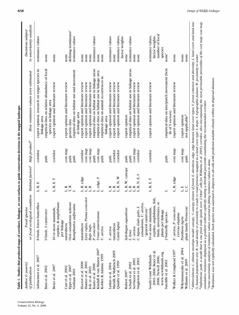
Ironically, many linkage designs lack the transparencythat should be a key advantage of a modeling approach.Key assumptions are often unstated and alternative ap-proaches are rarely mentioned. For example, in each of24 recent studies in which researchers used GIS proce-dures to identify connective habitats (Table 1), the ap-proach seemed reasonable, but each approach was differ-ent. Some of these differences reflect the different goalsof each effort, but some differences may reflect ignoranceof alternatives. Few of these studies explored sensitivityof the linkage design to alternatives.
We have helped produce 31 linkage designs for land-scapes in Arizona and southern California (South CoastWildlands 2003–2006; Beier et al. 2006, 2007). In our ex-perience, stakeholder discomfort with a poorly definedor justified model can result in objections to the entireapproach (Table 2). Conservation biologists should there-fore structure and explain their models in a way that ad-dresses, or at least acknowledges, key assumptions and al-ternatives. Explicitly recognizing choices along the roadto linkage design is essential to creating more rigorousconservation prescriptions.
Here we offer a roadmap of the assumptions andchoices involved in designing linkages for focal speciesbetween 2 or more wildlands. Thus we did not con-sider simulated annealing approaches (Andelman et al.1999; Possingham et al. 2000) or spatially explicit pop-
ulation models (Carroll et al. 2003) that take a broaderapproach to reserve design, simultaneously prioritizingland both for core-habitat blocks and linkages betweenthem. Because conservation biologists often are facedwith designing a linkage to connect 2 fixed reserve ar-eas, we addressed a family of approaches appropriate inmany landscapes. We concentrated on focal-species ap-proaches, rather than approaches intended to promotegeneral ecological connectivity (Hoctor et al. 2000; Carret al. 2002; Marulli & Mallarach 2005) or to encompass en-vironmental gradients or processes (Rouget et al. 2006).These latter approaches emphasize naturalness of landcover and may be more appropriate for depicting a coarseregional network than for designing a specific linkage.
Developing our procedures (South Coast Wildlands2003–2006; Beier et al. 2006, 2007) has been a tortuousjourney, with many decision points, or forks, encoun-tered along the road to linkage design. In some cases weexplored several paths before settling on one. At otherforks lack of time or data propelled us along a particularpath, leaving us wondering how different the resultantlinkage design would be at the end of a path not taken.A framework for linkage design can facilitate sharing oflessons and reduce the risk that a practitioner will takea particular fork without noticing alternative, and po-tentially better, options. We outline the questions facingthe analyst, describe and evaluate the ways analysts haveanswered these questions, and suggest better answers.Ultimately, we hope this framework will make linkagedesigns more defensible and successful.
The Basic Elements of Linkage Design
We define a corridor as a swath of land intended to al-low passage by a particular wildlife species between 2or more wildland areas. We use the term linkage to de-note connective land intended to promote movement ofmultiple focal species or propagation of ecosystem pro-cesses. We also use linkage as a generic term when thedistinction is unnecessary.
All published linkage designs for focal species (Table1) follow the same basic steps (Fig. 1). First stakehold-ers define their biological goals by identifying the land-scape and focal species. Then the analyst develops an
Conservation Biology
Volume 22, No. 4, 2008
838 Design of Wildlife Linkages
Tabl
e1.
Stud
ies
that
prod
uced
map
sof
corr
idor
s,lin
kage
s,or
cost
surf
aces
togu
ide
cons
erva
tion
deci
sion
sin
the
map
ped
land
scap
e.
Au
thor
&yea
r(s)
Foca
lsp
eci
es
Deci
sion
ssu
bje
ct
of
pu
bli
cati
on
or
foca
leco
logic
alco
ndit
ion
Ha
bit
at
fact
ors
aM
ap
pro
du
ctb
How
resi
sta
nce
va
lues
were
est
ima
ted
tou
nce
rta
inty
an
aly
sis
Ad
riae
nse
net
al.2
007
8b
ird
s,fo
rest
bu
tter
flie
sL,
R,E
corr
ido
rex
per
to
pin
ion
,res
earc
ho
nta
rget
spec
ies
inlin
kage
area
resi
stan
ceva
lues
Ban
iet
al.2
002
9b
ird
s,3
carn
ivo
res
Lp
ath
emp
iric
ald
ata
on
rela
tive
abu
nd
ance
of
foca
lsp
ecie
sin
linka
gear
ean
on
e
Bei
eret
al.2
007
10o
rm
ore
mam
mal
s,re
pti
les,
&am
ph
ibia
ns
per
linka
ge
L,R
,E,T
corr
ido
rex
per
to
pin
ion
and
liter
atu
rere
view
no
ne
Car
ret
al.2
002
nat
ura
lnes
sL,
Rco
stm
apex
per
to
pin
ion
and
liter
atu
rere
view
no
ne
Epp
set
al.2
007
Ovis
can
aden
sis
nels
on
iT
,Rp
ath
gen
etic
dat
ad
efin
ing
term
inu
sesc
Gra
ham
2001
Ra
mph
ast
os
sulf
ura
tus
Lp
ath
emp
iric
ald
ata
on
hab
itat
use
and
mo
vem
ent
inlin
kage
area
resi
stan
ceva
lues
Ho
cto
ret
al.2
000
nat
ura
lnes
sL,
R,e
dge
corr
ido
rex
per
to
pin
ion
and
liter
atu
rere
view
no
ne
Hu
nte
ret
al.2
003
Lyn
xru
fus,
Pu
ma
con
colo
rL,
Rco
stm
apex
per
to
pin
ion
and
liter
atu
rere
view
no
ne
Joly
etal
.200
3B
ufo
bu
foL,
Rco
stm
apex
per
to
pin
ion
and
liter
atu
rere
view
no
ne
Kau
tzet
al.2
006
P.co
nco
lor
Lp
ath
emp
iric
ald
ata
on
hab
itat
use
inlin
kage
area
sre
sist
ance
valu
esK
ind
all&
van
Man
en20
07U
rsu
sa
meri
can
us
L,ed
ge,F
cost
map
emp
iric
ald
ata
on
hab
itat
use
inlin
kage
area
no
ne
Ko
ble
r&
Ad
amic
1999
U.a
rcto
sL
pat
hem
pir
ical
dat
ao
nan
imal
occ
urr
ence
sin
linka
gear
ean
on
e
Lark
inet
al.2
004
U.a
rcto
sL,
Rp
ath
exp
ert
op
inio
nan
dlit
erat
ure
revi
ewre
sist
ance
valu
esM
aru
lli&
Mal
lara
ch20
05n
atu
raln
ess
L,R
corr
ido
rex
per
to
pin
ion
and
liter
atu
rere
view
no
ne
Qu
inb
yet
al.1
999
Ca
nis
lupu
sL,
R,N
,Wco
rrid
or
exp
ert
op
inio
nan
dlit
erat
ure
revi
ewre
sist
ance
valu
es,
fact
or
wei
ghts
Ru
ber
t20
07Sylv
ila
gu
sa
qu
ati
cus
L,R
,W,c
ano
py
pat
hex
per
to
pin
ion
no
ne
Sch
adt
etal
.200
2L.ly
nx
L,R
pat
hem
pir
ical
dat
ao
nh
abit
atu
sein
linka
gear
eas
resi
stan
ceva
lues
Serv
hee
net
al.2
001
U.a
rcto
sL,
Rco
stm
apex
per
to
pin
ion
and
liter
atu
rere
view
no
ne
Sin
glet
on
etal
.200
2C
.lu
pu
s,G
ulo
gu
lo,L.
can
aden
sis,
U.a
rcto
s,“g
ener
alca
rniv
ore
”
L,R
,N,E
,Sco
rrid
or
exp
ert
op
inio
nan
dlit
erat
ure
revi
ewn
on
e
Sou
thC
oas
tW
ildla
nd
s20
03–2
006;
Bei
eret
al.
2006
;New
ell2
006;
ww
w.s
cwild
lan
ds.
org
10o
rm
ore
mam
mal
s,re
pti
les,
amp
hib
ian
s,fi
sh,
bir
ds,
inve
rteb
rate
s,o
rp
lan
tsp
erlin
kage
L,R
,E,T
corr
ido
rex
per
to
pin
ion
and
liter
atu
rere
view
resi
stan
ceva
lues
,fa
cto
rw
eigh
ts,
nu
mb
ero
ffo
cal
spec
ies
Sutc
liffe
etal
.200
32
bu
tter
fly
spec
ies
Lp
ath
emp
iric
ald
ata
on
inte
rpat
chm
ove
men
t(b
est
fit
of
5ve
cto
rs)
no
nec
Wal
ker
&C
raig
hea
d19
97U
.a
rcto
s,P
.co
nco
lor,
Cerv
us
ela
ph
us
L,R
,ed
geco
stm
apex
per
to
pin
ion
and
liter
atu
rere
view
no
ne
Wik
ram
anay
ake
etal
.200
4P
an
thera
tigri
sL,
Eco
stm
apex
per
to
pin
ion
no
ne
Will
iam
set
al.2
005
pla
nt
fam
ilyP
rota
ceae
L,C
pat
hn
ot
app
licab
led
no
ne
aA
bbre
via
tion
s:C
,cl
ima
teen
velo
pe
model;
can
opy,%
can
opy
closu
reof
fore
st;E
,ele
va
tion
;edge,edge
betw
een
lan
dco
ver
types;
F,fo
rest
coh
esi
on
an
ddiv
ers
ity;L,la
nd
cover
an
dla
nd
use
;
N,h
um
an
popu
lati
on
size;R
,ro
ad
den
sity
or
pro
xim
ity
toro
ads
or
roa
dpre
sen
cem
apped
as
ala
nd
cover
type;S,sl
ope;T,to
pogra
ph
icfe
atu
re;W
,pro
xim
ity
tow
ate
r.bD
efi
nit
ion
s:pa
th,a
swa
thth
at
ison
epix
el
wid
e(p
ixels
were
2.9
-km
2ce
lls
for
Wil
lia
ms
et
al.
20
05
);co
rrid
or,
slic
een
com
pa
ssin
gth
em
ost
perm
ea
ble
perc
en
tile
sof
the
cost
ma
p;co
stm
ap,
cum
ula
tive
resi
sta
nce
dis
pla
yed
as
agra
die
nt
wit
hou
texpli
citl
yst
ati
ng
ath
resh
old
perc
en
tile
con
stit
uti
ng
the
reco
mm
en
ded
corr
idor.
cSom
eu
nce
rta
inty
an
aly
sis
of
resi
sta
nce
va
lues
occ
urr
ed
infi
ttin
gre
sist
an
ceva
lues
toda
ta.
dR
esi
sta
nce
wa
sn
ot
expli
citl
yca
lcu
late
d.E
ach
speci
es
wa
sa
ssu
med
todis
pers
eto
all
cells
wit
hpre
dic
ted
suit
able
clim
ate
wit
hin
its
dis
pers
aldis
tan
ce.
Conservation Biology
Volume 22, No. 4, 2008
Beier et al. 839
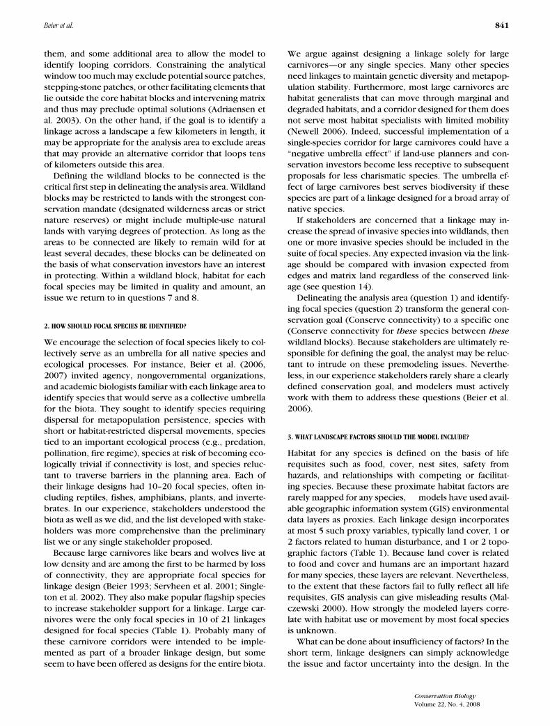
Table 2. Objections that may arise to focal-species approaches to linkage design when assumptions and choices are not clearly explained.∗
Relevant questionsObjection (Table 3)
A linkage designed to conserve focal species may fail to conserve ecological processes. 2, 11, 15A corridor designed for 1 or 2 large carnivores (often highly mobile habitat generalists) probably will not
serve other species.2
The model uncritically assumes that animals use the same rules to make movement decisions as they use toselect habitat.
5, 9
Animals choose habitat and make movement decisions on the basis of availability of food and mates and safetyfrom predators and hazards, but the model is derived from a few factors widely available in GIS format.
3
Because climate change will change the land-cover map used in the model, the linkage design will fail. 15The least-cost model always produces a “best” route, but the best may not be good enough to allow
movement and gene flow.14
Basing GIS models on movement is not appropriate for species that need several generations to move theirgenes through a linkage.
9
A linkage may facilitate movement of invasive species. 2, 11, 16The expense of implementing the linkage design outweighs its benefits. 14Least-cost modeling ignores some plants, insects, and birds whose movement cannot be modeled in this
framework.14
∗Linkage designers can address most issues by addressing relevant questions (second column).
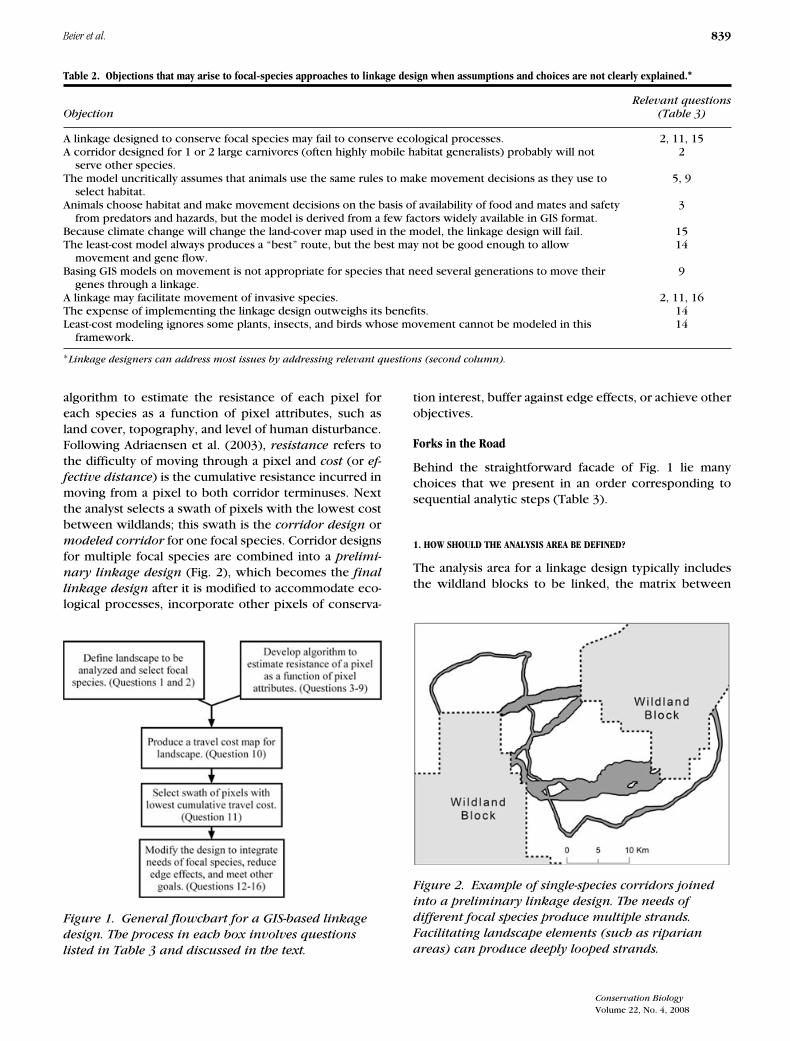
algorithm to estimate the resistance of each pixel foreach species as a function of pixel attributes, such asland cover, topography, and level of human disturbance.Following Adriaensen et al. (2003), resistance refers tothe difficulty of moving through a pixel and cost (or ef-
fective distance) is the cumulative resistance incurred inmoving from a pixel to both corridor terminuses. Nextthe analyst selects a swath of pixels with the lowest costbetween wildlands; this swath is the corridor design ormodeled corridor for one focal species. Corridor designsfor multiple focal species are combined into a prelimi-
nary linkage design (Fig. 2), which becomes the final
linkage design after it is modified to accommodate eco-logical processes, incorporate other pixels of conserva-
Figure 1. General flowchart for a GIS-based linkage
design. The process in each box involves questions
listed in Table 3 and discussed in the text.
tion interest, buffer against edge effects, or achieve otherobjectives.
Forks in the Road
Behind the straightforward facade of Fig. 1 lie manychoices that we present in an order corresponding tosequential analytic steps (Table 3).
1. HOW SHOULD THE ANALYSIS AREA BE DEFINED?
The analysis area for a linkage design typically includesthe wildland blocks to be linked, the matrix between
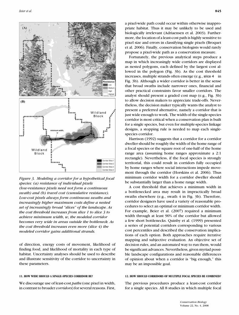
Figure 2. Example of single-species corridors joined
into a preliminary linkage design. The needs of
different focal species produce multiple strands.
Facilitating landscape elements (such as riparian
areas) can produce deeply looped strands.
Conservation Biology
Volume 22, No. 4, 2008
840 Design of Wildlife Linkages
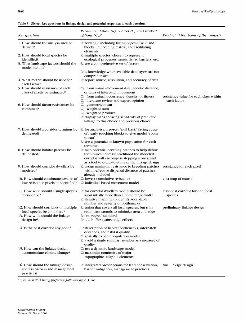
Table 3. Sixteen key questions in linkage design and potential responses to each question.
Recommendation (R), choices (C), and rankedKey question options (Cn)∗ Product at this point of the analysis
1. How should the analysis area bedefined?
R: rectangle including facing edges of wildlandblocks, intervening matrix, and facilitatingelements
2. How should focal species beidentified?
R: multiple species, chosen to representecological processes, sensitivity to barriers, etc.
3. What landscape factors should themodel include?
R: use a comprehensive set of factors
R: acknowledge when available data layers are notcomprehensive
4. What metric should be used foreach factor?
R: report source, resolution, and accuracy of data
5. How should resistance of eachclass of pixels be estimated?
C1: from animal-movement data, genetic distance,or rates of interpatch movement
C2: from animal occurrence, density, or fitnessC3: literature review and expert opinion
resistance value for each class withineach factor
6. How should factor resistances becombined?
C1: geometric meanC2: weighted sumC3: weighted productR: display maps showing sensitivity of predicted
linkage to this choice and previous choice
7. How should a corridor terminus bedelineated?
R: for analysis purposes, “pull back” facing edgesof nearly touching blocks to give model “roomto run”
R: use a potential or known population for eachterminus
8. How should habitat patches bedelineated?
R: map potential breeding patches to help defineterminuses, increase likelihood the modeledcorridor will encompass stepping stones, andas a tool to evaluate utility of the linkage design
9. How should corridor dwellers bemodeled?
R: assign minimum resistance to breeding patcheswithin effective dispersal distance of patchesalready included
resistance for each pixel
10. How should continuous swaths oflow-resistance pixels be identified?
C: lowest cumulative resistanceC: individual-based movement model
cost map of matrix
11. How wide should a single-speciescorridor be?
R: for corridor dwellers, width should besubstantially more than a home range width
least-cost corridor for one focalspecies
R: iterative mapping to identify acceptablenumber and severity of bottlenecks
12. How should corridors of multiplefocal species be combined?
R: union that covers all focal species, but trimredundant strands to minimize area and edge
preliminary linkage design
13. How wide should the linkagedesign be?
R: “no regret” standardR: add buffer against edge effects
14. Is the best corridor any good? C: description of habitat bottlenecks, interpatchdistances, and habitat quality
C: spatially explicit population modelR: avoid a single summary number as a measure of
quality15. How can the linkage design
accommodate climate change?C: use a dynamic landscape modelC: maximize continuity of major
topographic–edaphic elements
16. How should the linkage designaddress barriers and managementpractices?
R: integrated prescriptions for land conservation,barrier mitigation, management practices
final linkage design
∗n, rank, with 1 being preferred, followed by 2, 3, etc.
Conservation Biology
Volume 22, No. 4, 2008
Beier et al. 841
them, and some additional area to allow the model toidentify looping corridors. Constraining the analyticalwindow too much may exclude potential source patches,stepping-stone patches, or other facilitating elements thatlie outside the core habitat blocks and intervening matrixand thus may preclude optimal solutions (Adriaensen etal. 2003). On the other hand, if the goal is to identify alinkage across a landscape a few kilometers in length, itmay be appropriate for the analysis area to exclude areasthat may provide an alternative corridor that loops tensof kilometers outside this area.
Defining the wildland blocks to be connected is thecritical first step in delineating the analysis area. Wildlandblocks may be restricted to lands with the strongest con-servation mandate (designated wilderness areas or strictnature reserves) or might include multiple-use naturallands with varying degrees of protection. As long as theareas to be connected are likely to remain wild for atleast several decades, these blocks can be delineated onthe basis of what conservation investors have an interestin protecting. Within a wildland block, habitat for eachfocal species may be limited in quality and amount, anissue we return to in questions 7 and 8.
2. HOW SHOULD FOCAL SPECIES BE IDENTIFIED?
We encourage the selection of focal species likely to col-lectively serve as an umbrella for all native species andecological processes. For instance, Beier et al. (2006,2007) invited agency, nongovernmental organizations,and academic biologists familiar with each linkage area toidentify species that would serve as a collective umbrellafor the biota. They sought to identify species requiringdispersal for metapopulation persistence, species withshort or habitat-restricted dispersal movements, speciestied to an important ecological process (e.g., predation,pollination, fire regime), species at risk of becoming eco-logically trivial if connectivity is lost, and species reluc-tant to traverse barriers in the planning area. Each oftheir linkage designs had 10–20 focal species, often in-cluding reptiles, fishes, amphibians, plants, and inverte-brates. In our experience, stakeholders understood thebiota as well as we did, and the list developed with stake-holders was more comprehensive than the preliminarylist we or any single stakeholder proposed.
Because large carnivores like bears and wolves live atlow density and are among the first to be harmed by lossof connectivity, they are appropriate focal species forlinkage design (Beier 1993; Servheen et al. 2001; Single-ton et al. 2002). They also make popular flagship speciesto increase stakeholder support for a linkage. Large car-nivores were the only focal species in 10 of 21 linkagesdesigned for focal species (Table 1). Probably many ofthese carnivore corridors were intended to be imple-mented as part of a broader linkage design, but someseem to have been offered as designs for the entire biota.
We argue against designing a linkage solely for largecarnivores—or any single species. Many other speciesneed linkages to maintain genetic diversity and metapop-ulation stability. Furthermore, most large carnivores arehabitat generalists that can move through marginal anddegraded habitats, and a corridor designed for them doesnot serve most habitat specialists with limited mobility(Newell 2006). Indeed, successful implementation of asingle-species corridor for large carnivores could have a“negative umbrella effect” if land-use planners and con-servation investors become less receptive to subsequentproposals for less charismatic species. The umbrella ef-fect of large carnivores best serves biodiversity if thesespecies are part of a linkage designed for a broad array ofnative species.
If stakeholders are concerned that a linkage may in-crease the spread of invasive species into wildlands, thenone or more invasive species should be included in thesuite of focal species. Any expected invasion via the link-age should be compared with invasion expected fromedges and matrix land regardless of the conserved link-age (see question 14).
Delineating the analysis area (question 1) and identify-ing focal species (question 2) transform the general con-servation goal (Conserve connectivity) to a specific one(Conserve connectivity for these species between these
wildland blocks). Because stakeholders are ultimately re-sponsible for defining the goal, the analyst may be reluc-tant to intrude on these premodeling issues. Neverthe-less, in our experience stakeholders rarely share a clearlydefined conservation goal, and modelers must activelywork with them to address these questions (Beier et al.2006).
3. WHAT LANDSCAPE FACTORS SHOULD THE MODEL INCLUDE?
Habitat for any species is defined on the basis of liferequisites such as food, cover, nest sites, safety fromhazards, and relationships with competing or facilitat-ing species. Because these proximate habitat factors arerarely mapped for any species, so models have used avail-able geographic information system (GIS) environmentaldata layers as proxies. Each linkage design incorporatesat most 5 such proxy variables, typically land cover, 1 or2 factors related to human disturbance, and 1 or 2 topo-graphic factors (Table 1). Because land cover is relatedto food and cover and humans are an important hazardfor many species, these layers are relevant. Nevertheless,to the extent that these factors fail to fully reflect all liferequisites, GIS analysis can give misleading results (Mal-czewski 2000). How strongly the modeled layers corre-late with habitat use or movement by most focal speciesis unknown.
What can be done about insufficiency of factors? In theshort term, linkage designers can simply acknowledgethe issue and factor uncertainty into the design. In the
Conservation Biology
Volume 22, No. 4, 2008
842 Design of Wildlife Linkages
long term, the scientific community can encourage devel-opment of maps of soils, rock outcrops, permanent watersources, and other factors known to affect habitat use byfocal species. In our work in the southwestern UnitedStates, these factors are important for focal species suchas pronghorn (Antilocapra americana), bighorn (Ovis
canadensis), prairie dogs (Cynomys sp.), and many rep-tiles. With reliable coverages of such features, modelscould be improved immediately.
4. WHAT METRIC SHOULD BE USED FOR EACH FACTOR?
Once factors are chosen, the analyst must chooseresistance-relevant metrics for each factor. Metrics can becategorical (e.g., land-cover types, topographic classes)or continuous (e.g., elevation, distance from water). Inmost models (Table 1), each continuous variable (e.g.,elevation) is converted into a categorical variable witha handful of classes (e.g., below, within, and above thepublished elevational limits of the species). Land-coverdata may be available in a layer with 20–30 coarse classes(National Land Cover Database in the United States) or70–100 classes (National Gap Analysis Program data lay-ers in the United States).
Most wildlife habitat studies in which these maps wereused present the data as if they represented reality (Glenn& Ripple 2004). Nevertheless, classification accuracy istypically 60% to 80% (Yang et al. 2001), and digital mapsdeveloped from different remotely sensed images pro-duce markedly different depictions of vegetation (Glenn& Ripple 2004). We recommend that practitioners re-port resolution, accuracy, and source for land-cover data.We have found it useful to lump GAP classes into 25–50 classes because the GAP accuracy assessments indi-cate that many errors involve confusion between closelyrelated land covers. Pooling these closely related typesincreases the classification accuracy of the map.
In most linkage designs, human disturbance was mea-sured by road density within a moving window. Unfor-tunately, despite the seeming scale invariance of lengthper length squared, the calculated value of road densitychanges nonintuitively with the size of the moving win-dow (D. R. Majka, unpublished data). Thus, it is difficult toreliably estimate resistance for road density classes, andpublished estimates of animal occurrence with respectto road density cannot be translated to a different-sizedmoving window. Distance to the nearest road avoids thisproblem and may be a more appropriate road-related met-ric of human disturbance. We discourage the practice ofcreating a separate class for road pixels that contain apotential crossing structure (e.g., bridge, culvert) and as-signing a low resistance to those pixels. This practiceforces the modeled corridor through the crossing struc-ture, even when the structure is located in otherwisepoor habitat. Thus it prevents the planner from identify-ing optimal locations for road-crossing structures.
Models can include one or more topographic metrics,such as elevation, aspect, insolation, slope, ruggedness,or topographic position, all of which are derived from acommon set of digital elevation data. Some topographicmetrics (e.g., elevation and aspect) probably affect ani-mal movement by determining land cover, or (for poik-ilotherms) by influencing the thermal environment ofthe species. Other topographic metrics such as rugged-ness and topographic position may directly affect ani-mal movements. Topographic position can be estimatedby classifying pixels into any number of classes, such asslope, ridgetop, or valley bottom (algorithms providedby J. Jenness [http://www.jennessent.com/]). The algo-rithms for ruggedness and topographic position requirespecifying window size (scale). Although it is appealingto model topography from the perspective of the focalspecies, the scale at which organisms assess topographyis usually unknown. More important, most cost valuesare assigned by making inferences from scientific publi-cations, which usually report animal response to topog-raphy as it was perceived by the human researcher. Dick-son and Beier (2007) illustrate the use of topographicposition and discuss the issue of window size and otherprocedural decisions. We encourage uncertainty anal-ysis to address how these decisions affect a modeledcorridor.
5. HOW SHOULD RESISTANCE OF EACH CLASS OF PIXELS BE ESTIMATED?
Setting resistance values is “the link between the non-ecological GIS information and the ecological-behavioralaspects of the mobility of the organism or process” (Adri-aensen et al. 2003:234). As such it has received moreattention from linkage designers than any other issue wediscuss here.
Resistance of each class of land use, topography, orhuman disturbance is usually determined on the basisof expert opinion and literature review. Clevenger et al.(2002) emphasize the poor performance of expert opin-ion if it is not combined with literature review. In allpublished linkage designs, practitioners assigned scoreson an arbitrary scale (typically 0 to 1, or 1 to 100). Be-cause most of the relevant literature is on habitat userather than animal movement (Chetkiewicz et al. 2006),one end of the scale reflects low resistance and high habi-tat quality, and the other end of the scale reflects highresistance and low habitat quality. In other words, one setof scores is interpreted as both a resistance model and ahabitat-suitability model. This complementarity betweenresistance and habitat suitability reflects the assumptionthat animals choose travel routes on the basis of the samefactors they use to choose habitat (Chetkiewicz et al.2006). Although this seems reasonable, it may not alwaysbe true. For instance, Horskins et al. (2006) demonstratedthat one corridor failed to provide gene flow for 2 speciesthat occurred and probably bred within the corridor.
Conservation Biology
Volume 22, No. 4, 2008
Beier et al. 843
Following Walker and Craighead (1997), we urge linkagedesigners to explicitly state this as a crucial assumptionand acknowledge that the assumption is untested.
Four types of empirical data (species occurrences, an-imal movement paths, interpatch movement rates, andgenetic patterns among patches) can be analyzed in aresource-selection framework to provide estimates of re-sistance better than estimates from literature review andexpert opinion. Unfortunately, resistance estimates de-rived from each type of data are subject to considerableuncertainty. Because this uncertainty is central to the in-terpretation of all resistance-based models, we address itin a separate section (“Subjective Translation and OtherProblems”).
Several designers have used uncertainty analyses toassess the impact of uncertainty in resistance estimates(Quinby et al. 1999; Schadt et al. 2002; Larkin et al. 2004;Newell 2006; Adriaensen et al. 2007). The results of mostof these studies suggest that the location of the mod-eled corridor does not change significantly as long as therank order of resistance values is assumed correct. Nev-ertheless, Schadt et al. (2002) attributed much of thisinsensitivity to the lack of alternative corridor locationsin their highly urbanized potential linkage areas. In anextensive uncertainty analysis of the approach used byBeier et al. (2006), Newell (2006) found that modeledcorridors were stable for 5 of 8 focal species in a large (50× 35 km) potential linkage area relatively unconstrainedby existing urbanization.
Uncertainty analysis can estimate the impact of uncer-tainty only for a particular focal species and landscape.Perhaps after many such analyses, general rules will be es-tablished about the types of species and landscapes thatare insensitive to uncertainty. Until then we recommendthat corridor designers routinely incorporate uncertaintyanalysis and present maps of model results under themost strongly divergent estimates of resistance, as Quinbyet al. (1999) did.
6. HOW SHOULD FACTOR RESISTANCES BE COMBINED?
To estimate the overall resistance of a pixel, the analystmust combine resistance due to land cover with resis-tance due to human disturbance and other factors. To doso, the analyst must choose an arithmetic operation andassign a weight to each factor.
Most linkage designers have used a weighted sum tocombine factor resistances, but Singleton et al. (2002)used a weighted product and Beier et al. (2007) useda weighted geometric mean. The geometric mean bet-ter reflects situations in which one factor limits wildlifemovement in a way that cannot be compensated for by alower resistance for another factor (U.S. Fish & WildlifeService 1981).
Regardless of arithmetic operation, each factor is as-signed a weight reflecting its contribution to the overall
resistance of a pixel. In all published linkage designs,weights seem to have been assigned solely by expertopinion. The expert’s task is complicated by the fact thata factor’s weight reflects not only its importance, but alsothe factor’s range of variation and units of measurement(Malczewski 2000). Use of a common scale (e.g., resis-tance units of 1–100) for each factor is common practicein least-cost modeling and eliminates differences amongfactors in range and units of measurement. Nevertheless,this presupposes that the resistance values for each fac-tor were assigned in a way that compensates for differ-ences among factors in range and units of measurement.Lacking evidence for this presupposition, we recommendthat uncertainty analysis consider the simultaneous im-pact of uncertainty in both weights and class resistancescores, as was done by Quinby et al. (1999) and Newell(2006).
Although uncertainty analysis is a helpful short-term so-lution, in the future we hope that empirical, multivariateresource-selection studies will directly estimate weightsand resistances and will suggest the proper way to com-bine factor resistances. Such studies could also revealimportant interactions between factors.
7. HOW SHOULD A CORRIDOR TERMINUS BE DELINEATED?
A terminus is that part of a wildland block that formsor anchors one end of a modeled corridor. A terminuscan be defined as a point (pixel), a linear edge (e.g., thewildland boundary), or a patch (e.g., a patch of high-quality focal-species habitat within the wildland block).There can be more than one potential terminus in eachwildland block.
Some linkage designs use each wildland block in its en-tirety as a terminus for each single-species analysis. Never-theless, in our experience this procedure sometimes pro-duces a corridor that connects to a part of the wildlandblock far from any potential habitat for the focal species.This unreasonable result can be avoided by restrictingterminuses to patches of known or potential breedinghabitat (next section) within each wildland block.
Because distance is an important part of algorithmsthat are based on effective distance, in cases in which2 wildland blocks nearly touch at one or more loca-tions, these algorithms tend to identify the narrowestgap as the best corridor, even if the modeled corridoris low in habitat value or movement potential. To avoidthis problem, we recommend giving the model “room torun” by identifying terminuses well inside the wildlandblocks, behind parallel lines a few kilometers apart. Evenif this modification does not change the modeled cor-ridor for any focal species, it will demonstrate that themodeled corridor is not merely an artifact of boundaryproximity.
Conservation Biology
Volume 22, No. 4, 2008
844 Design of Wildlife Linkages
8. HOW SHOULD HABITAT PATCHES BE DELINEATED?
Habitat patches are areas of habitat that can support re-production by the focal species; they may occur withinwildland blocks or matrix. Although linkage design doesnot require delineation of habitat patches, in our experi-ence it is useful to delineate habitat patches as steppingstones within the matrix (next section), as terminuseswithin the wildland blocks (previous section), and asuseful metrics for assessing functionality of a modeledlinkage design (see question 14).
To delineate habitat patches, the analyst must specify asuitability threshold for habitat quality, the minimum areaof suitable habitat necessary to sustain a breeding pair orpopulation, and how nonhabitat pixels (at patch edges orislets within a patch) affect habitat quality (e.g., via edgeeffects). South Coast Wildlands (2003–2006), SouthernRockies Ecosystem Project (2005), Beier et al. (2007),and Girvetz and Greco (2007) illustrate procedures toidentify pixels that are “good enough, big enough, andclose enough together” to function as a habitat patch. Todate, there has been no formal uncertainty analysis to de-termine how uncertainty in each of these 3 proceduresaffects either the map of habitat patches or the modeledcorridor. Although we advocate such uncertainty analy-sis, we believe the procedures currently in use providereasonable patch maps and that using these maps is bet-ter than ignoring the distribution of breeding habitat inthe planning area.
9. HOW SHOULD CORRIDOR DWELLERS BE MODELED?
An unstated assumption in many corridor models is thatan individual animal can move between wildland blocksin a single movement event of a few hours to a fewweeks. Beier and Loe (1992) called such animals pas-sage species and pointed out that other focal species—corridor dwellers—require more than one generation tomove their genes between wildland blocks. They basedtheir distinction on an interaction between the speciesand the landscape; thus, a particular species would bea passage species if the habitat blocks were within dis-persal distance, but would be a corridor dweller in an-other landscape with habitat blocks more than one dis-persal distance away. Corridor dwellers must find suitablebreeding opportunities within the linkage.
To model movement by corridor dwellers, Wikra-manayake et al. (2004), Beier et al. (2007), and Adriaensenet al. (2007) assigned the lowest resistance value tohabitat patches (previous section). We recommend thisprocedure when modeling a species with a few habitatpatches imbedded in a matrix dominated by poor habi-tat. In such situations the procedure tends to produce acorridor that links those patches in stepping-stone fash-ion. Nevertheless, if the habitat quality in a large fractionof the matrix is near the threshold between suitable and
unsuitable, a slight decrease in the threshold can causemost of the matrix to be mapped as a habitat patch, re-sulting in a highly linear corridor that fails to include thehighest-quality habitat. In these situations we discourageuse of this procedure unless the analyst is confident thatthe threshold is precisely known.
The procedures of Wikramanayake et al. (2004) andBeier et al. (2007) could be improved by assigningthe lowest resistance value only to potential breedingpatches within effective dispersal distance of other po-tential breeding patches in the linkage. Nevertheless, “ef-fective dispersal distance” in this context means dispersaldistance in suboptimal habitat, and such data are avail-able for only a few species. Even if such data (i.e., afrequency distribution of dispersal distances) were avail-able, the data would not allow the analyst to infer theexact threshold at which interpatch connectivity is lost.A rigorous but data-hungry approach is suggested by vanLangevelde (2000), who estimated this threshold distancefrom a time series of patch occupancy.
10. HOW SHOULD CONTINUOUS SWATHS OF LOW-RESISTANCE
PIXELS BE IDENTIFIED?
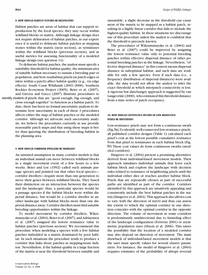
Low-resistance pixels may not form a continuous swath(Fig. 3). To identify well-connected low-resistance pixels,all published corridor designs (Table 1) calculated eachpixel’s cost as the lowest possible cumulative resistancefrom that pixel to terminuses in each habitat block (Fig.3). These cost values do form continuous swaths (mod-eled corridors).
Hargrove et al. (2004) present a promising alternativederived from individual-based movement models. Theirapproach simulates individual animals that leave eachhabitat block and explore the landscape with decisionrules related to resistance of neighboring pixels until theindividual either dies or reaches another habitat block.Pixels that are repeatedly chosen as part of successfulpaths are identified as part of the corridor. Corridorsidentified by this approach are intuitively appealing andconsistently include the best habitat patches in the ma-trix (Hargrove et al. 2004). This approach also allows costto vary with the direction of travel and thus can assessthe extent to which the optimal corridor in one direc-tion coincides with the optimal corridor in the oppositedirection. The volume of movement in some corridorsis predominantly unidirectional due to funneling effectof the landscape configuration (Ferreras 2001) or asym-metric population sizes (Dixon et al. 2006). This raisesthe possibility that the location of a modeled corridormay also depend on direction of movement. The maindrawback of individual-based movement models is thatthe user must specify values for several elusive param-eters. For instance, the model of Hargrove et al. (2004)requires estimates of the probability of abrupt reversal
Conservation Biology
Volume 22, No. 4, 2008
Beier et al. 845
Figure 3. Modeling a corridor for a hypothetical focal
species: (a) resistance of individual pixels
(low-resistance pixels need not form a continuous
swath) and (b) travel cost (cumulative resistance).
Low-cost pixels always form continuous swaths and
increasingly higher maximum costs define a nested
set of increasingly broad “slices” of the landscape. As
the cost threshold increases from slice 1 to slice 3 to
achieve minimum width, w, the modeled corridor
becomes very wide in areas outside the bottleneck. As
the cost threshold increases even more (slice 4) the
modeled corridor gains additional strands.
of direction, energy costs of movement, likelihood offinding food, and likelihood of mortality in each type ofhabitat. Uncertainty analyses should be used to describeand illustrate sensitivity of the corridor to uncertainty inthese parameters.
11. HOW WIDE SHOULD A SINGLE-SPECIES CORRIDOR BE?
We discourage use of least-cost paths (one pixel in width,in contrast to broader corridors) for several reasons. First,
a pixel-wide path could occur within otherwise inappro-priate habitat. Thus it may be unlikely to be used andbiologically irrelevant (Adriaensen et al. 2003). Further-more, the location of a least-cost path is highly sensitive topixel size and errors in classifying single pixels (Broquetet al. 2006). Finally, conservation biologists would rarelypropose a pixel-wide path as a conservation measure.
Fortunately, the previous analytical steps produce amap in which increasingly wide corridors are displayedas nested polygons, each defined by the largest cost al-lowed in the polygon (Fig. 3b). As the cost thresholdincreases, multiple strands often emerge (e.g., swath 3 inFig. 3b). Although a wider corridor is better in the sensethat broad swaths include narrower ones, financial andother practical constraints favor smaller corridors. Theanalyst should present a graded cost map (e.g., Fig. 3b)to allow decision makers to appreciate trade-offs. Never-theless, the decision maker typically wants the analyst topresent a preferred alternative, namely a corridor that isjust wide enough to work. The width of the single-speciescorridor is most critical when a conservation plan is builtfor a single species, but even for multiple-species linkagedesigns, a stopping rule is needed to map each single-species corridor.
Harrison (1992) suggests that a corridor for a corridordweller should be roughly the width of the home range ofa focal species or the square root of one-half of the homerange area (assuming home ranges approximate a 2:1rectangle). Nevertheless, if the focal species is stronglyterritorial, this could result in corridors fully occupiedby home ranges where social interactions impede move-ment through the corridor (Horskins et al. 2006). Thusminimum corridor width for a corridor dweller shouldbe substantially larger than a home range width.
A cost threshold that achieves a minimum width ina bottlenecked area may result in impractically broadswaths elsewhere (e.g., swath 4 in Fig. 3b). Therefore,corridor designers have used a variety of reasonable pro-cedures to select an optimal or minimum corridor width.For example, Beier et al. (2007) required a minimumwidth through at least 90% of the corridor but alloweda few short bottlenecks. Quinby et al. (1999) presenteda series of potential corridors corresponding to variouscost percentiles and described the conservation implica-tions of each option. Both approaches require iterativemapping and subjective evaluation. An objective set ofdecision rules, and an automated way to run them, wouldbe significant advances. Nevertheless, given myriad possi-ble landscape configurations and reasonable differencesof opinion about when a corridor is “big enough,” thismay be an impossible goal.
12. HOW SHOULD CORRIDORS OF MULTIPLE FOCAL SPECIES BE COMBINED?
The previous procedures produce a least-cost corridorfor a single species. All 8 studies in which multiple focal
Conservation Biology
Volume 22, No. 4, 2008
846 Design of Wildlife Linkages
species were used (Table 1) present separate maps foreach focal taxon. Only Singleton et al. (2002), Beier et al.(2006, 2007), and Adriaensen et al. (2007) joined thesingle-species corridors into a multiple-species linkagedesign. Singleton et al. (2002) used the median resistancevalue for each pixel type across the 4 focal species to de-velop a “general carnivore model.” We discourage thisapproach, or other types of model averaging, becausethe general linkage may encompass none of the single-species corridors. Beier et al. (2006) took the union of allpixels included in one or more single-species corridor.Although this procedure fulfilled its goal of “no speciesleft behind,” it risked being larger than needed and thusneedlessly expensive. To remedy this, Beier et al. (2007)trimmed pixels that served only one species as long asthe deletion did not significantly affect corridor length oraverage habitat quality for that species. South Coast Wild-lands (2003–2006) and Beier et al. (2007) also enlargedthe multispecies linkage to include species-specific habi-tat patches if such an addition decreased the interpatchdistances that dispersers would need to cross. Their trim-ming and adding procedures were subjective and onlyweakly quantitative. We encourage others to developmore rigorous procedures to minimize acquisition costs(area) and management costs (edge) without degradingthe ability of the linkage design to serve all focal species.
13. HOW WIDE SHOULD THE LINKAGE BE?
Wide linkages are beneficial because they provide formetapopulations of linkage-dwelling species (includingthose not used as focal species); reduce pollution intoaquatic linkages; reduce edge effects due to pets, light-ing, noise, nest predation, nest parasitism, and invasivespecies; provide an opportunity to conserve ecologicalprocesses such as natural fire regimes; and help the biotarespond to climate change. For these reasons, some or allstrands of the linkage design should be wide enough toprovide these benefits. Negative edge effects are biologi-cally significant at distances of up to 300 m in terrestrialsystems (25 studies summarized by Environmental LawInstitute [2003]) and 50 m in aquatic systems (88 studiesin the same review). We recommend the use of thesedistances as buffers added to the edges of a draft linkagedesign to minimize edge effects in the modeled linkage.In some situations, topographic features such as steepcliffs alongside a canyon-bottom linkage may block edgeeffects, reducing the need for a buffer. None of the de-signs in Table 1 rigorously justified a minimum widthneeded to conserve ecological processes because appar-ently there is no relevant literature.
Real-estate developers seeking government approvalfor their plans typically frame this question as, How nar-row a linkage strand might possibly be useful to the fo-cal species? Perhaps because they spend so much timenegotiating with developers, some government planners
frame the question the same way. In our view this is anal-ogous to asking an engineer, What are the fewest numberof rivets that might keep this wing on the airplane? Weurge linkage designers to reframe the question as, What isthe narrowest width that is not likely to be regretted afterthe adjacent area is converted to human uses? Althoughthis no-regret standard is subjective, corridor designershave to draw the line somewhere, and we have found ithelpful to reframe the issue this way.
14. IS THE BEST CORRIDOR ANY GOOD?
Least-cost procedures of GIS will always produce a least-cost corridor or path—even if the best is entirely inad-equate for the focal species. Therefore linkage designsshould assess how well the linkage design serves eachspecies and how connectivity provided by the linkage af-ter development compares with other benchmarks (suchas connectivity under existing conditions, an alternativelinkage design, or conversion of all matrix land to humanuses). A conventional estimate of cost-weighted distanceis a poor assessment metric because it does not indicatethe level of interpatch movement or gene flow.
Until reliable resistance measures are developed, link-age designers must provide conservation investors andother stakeholders with meaningful descriptions of howwell the linkage design is expected to serve each focalspecies. For example, Larkin et al. (2004) report the num-ber of road crossings and the number and severity of bot-tlenecks in alternative corridors. Beier et al. (2007) pro-vide frequency distributions of species-specific habitatquality in the linkage design and describe the longest dis-tances an individual animal would have to move betweenpotential breeding patches. In cases in which the inter-patch distances exceeded the estimated dispersal abil-ity of the species, South Coast Wildlands (2003–2006)and Beier et al. (2007) acknowledge that the linkage de-sign probably would not provide meaningful connectivityfor that species. South Coast Wildlands (2003–2006) andBeier et al. (2007) also used these descriptors to evaluatelinkage utility for species (some birds, plants, and volantinsects) for which habitat patches could be mapped butwhose interpatch movement could not be modeled. Fur-thermore, they added patches of suitable habitat to thelinkage design when such addition significantly reducedthe length of interpatch dispersal movements requiredfor one of these species.
J. Jenness recently developed an ArcMap extension(http://www.corridordesign.org/) that generates statis-tics on bottlenecks, interpatch distances, habitat qual-ity, and other metrics for any linkage design polygon ofinterest to stakeholders. These statistics can help conser-vation investors compare the biological optimum in a setof parcels meeting a cost constraint or other conservationgoal.
Conservation Biology
Volume 22, No. 4, 2008
Beier et al. 847
15. HOW CAN THE LINKAGE DESIGN ACCOMMODATE CLIMATE CHANGE?
All least-cost models include natural vegetation as a keydriver; vegetation in turn is determined largely by climate,soils, and topography. Within the next 50 years, one ofthese factors, climate, will change enough to cause majorshifts and reassembly of vegetation communities (Inter-governmental Panel on Climate Change 2001: Section5.2.2.2). Williams et al. (2005) designed a linkage to al-low endemic plants to shift their geographic range in re-sponse to climate change. Their procedure modeled suit-able habitat at intervals of a decade and identified spatiallyand temporally contiguous chains of 2.9-km2 grid cellswith suitable habitat. Beier et al. (2006, 2007) assumedthat a diversity of topographic elements (combinations ofelevation, slope, and aspect, such as high-elevation flats,north-facing slopes, or lowland flats) would support rel-atively continuous strands of whatever native vegetationcommunities will be present after climate change. Theytherefore evaluated their linkage designs for continuityof major topographic elements and expanded the link-age design to increase such continuity as needed. Theirprocedure would be improved by considering soil typein addition to topography and by the use of an objectivemultivariate procedure to identify the major edaphic–topographic elements in a region. There is enormousroom for innovation on this important issue.
16. HOW SHOULD THE LINKAGE DESIGN ADDRESS BARRIERS
AND MANAGEMENT PRACTICES?
We advocate that linkage designs should comprehen-sively address land conservation, barrier mitigation, andland management practices. Unfortunately, most pub-lished linkage designs have one product, namely a maphighlighting lands for conservation. There is a largelyseparate literature on wildlife-friendly highway crossingstructures and other mitigations for highways and canals(e.g., National Highway Cooperative Research Program2004; National Research Council 2005; Ventura County2005; online proceedings of the International Confer-ences on Ecology and Transportation [www.icoet.net/]).Conserving land will not create a functional linkage ifmajor barriers are not mitigated, an excellent crossingstructure will not create a functional linkage if the adja-cent land is urbanized, and an integrated project of landacquisition and highway mitigation could be jeopardizedby inappropriate practices (e.g., predator control, fenc-ing, artificial night lighting).
South Coast Wildlands (2003–2006) and Beier et al.(2007) used field observations to develop fine-scale rec-ommendations for crossing structures and managementpractices to restore native vegetation and minimize theimpact of exotic species, fences, pets, livestock, and arti-ficial night lighting. In our experience this is the sectionof the report most avidly read and used by managers. Ac-
cordingly, the main body of each of our reports consistsof a short (approximately 5 pages) description of how thelinkage design will serve focal species (question 14) and10–20 pages of management recommendations (question16). Everything else is relegated to lengthy appendices.Georeferenced photographs help illustrate important rec-ommendations.
Management recommendations are especially impor-tant where people already live in or adjacent to thelinkage design and must be engaged as its stewards. Anemerging issue is how to mitigate the impact of solid-steelfences, mowed strips, and stadium lighting designed todiscourage human traffic on international borders.
Subjective Translation and Other Issuesin Estimating Resistance
We introduce the term subjective translation to label animportant problem that affects most resistance estimates.The problem is that resource selection metrics are usuallytranslated into resistance estimates in a subjective way.The problem is most obvious for estimates derived fromthe literature and expert opinion, in which the analyst as-signs a resistance score to each resource state by extrap-olating from the literature on resource selection. Studiesof resource selection produce results such as a rankedlist of resource classes, probability of the species occur-ring in each class, a ratio or difference between use andavailability of each class, number of animal occurrencesin each class, or the mean distance from animal locationsto the nearest occurrence of each class (Millspaugh &Marzluff 2001). If the focal animal is twice as likely tooccur in pixel type A as in pixel type B, it is tempting toinfer that B has twice the resistance of A. Nevertheless,such inference is valid only if the relationship betweenresistance and probability of occurrence is a linear, ratherthan exponential, logarithmic, or other function. Thereis no objective basis for choosing any one of these func-tions. Indeed, few linkage analysts even state how theytranslate resource-selection metrics into resistance. Evenwhen they do (e.g., Ferreras 2001), the decision remainssubjective.
Empirical data collected in the landscape of interestshould provide a better basis than literature review forestimating resistance of various pixel classes, but sometypes of empirical data are still subject to the subjectivetranslation problem. We considered 4 types of empiri-cal data: species occurrence, animal movement, rates ofinterpatch movement, and genetic distances among pop-ulations. Kobler and Adamic (1999), Ferreras (2001), Baniet al. (2002), and Adriaensen et al. (2007) estimated re-sistance of land-use classes on the basis of empirical dataon occurrence or abundance of focal species in eachland-use class. Their approaches, and other approaches
Conservation Biology
Volume 22, No. 4, 2008
848 Design of Wildlife Linkages
derived from resource-selection studies in the region ofinterest, improve on literature review or expert opin-ion because they use animal observations in the linkageplanning area, but they are still affected by the subjective-translation problem.
Data on animal movement in the linkage area can yieldresistance estimates free of subjective translation. Gra-ham (2001) used data on daily movements of Keel-billedToucans (Ramphastos sulfuratus) to assign resistancescores to 3 coarse land-cover classes. Graham’s approachcould be improved by including a more formal estima-tion procedure, a larger number of resource classes, anddata on individuals moving between patches of breed-ing habitat (rather than daily movement within a homerange).
If interpatch movement rates are a function of the resis-tance of each pixel type in the matrix between patches,multivariate methods can identify the set of resistancevalues (a vector in matrix algebra) that best explainsobserved movement rates. Nevertheless, Sutcliffe et al.(2003) noted 2 difficulties. First, unless the researchersamples the entire geographic range of the metapopu-lation, estimates will be distorted due to (unmeasured)movements from patches outside the study area butwithin the interacting group of patches. Second, if theresistance vector includes 3 or more classes, it may beimpossible to solve for a single best vector. Sutcliffe et al.(2003) addressed this problem by starting with a handfulof likely vectors derived from ecological knowledge ofthe focal species and determining which of these vec-tors was most consistent with observed rates of inter-patch movement. Similarly, Verbeylen et al. (2003) usedan information-theory approach to select which of 36potential resistance vectors was most consistent with ob-served occupancy of putative sink patches. These ad hocprocedures were reasonable, but it is impossible to knowwhether the set of test vectors included the true vector orto obtain a unique mathematical solution if the numberof resistances exceeds the number of patch pairs withdata.
Epps et al. (2005) used genetic distances among pop-ulations to estimate the resistance that highways poseto movement by bighorn sheep by assigning each pixelof the matrix to 1 of 2 resistance classes (one for thehighway, one for all other matrix pixels). Gerlach andMusolf (2000) similarly estimated resistance of a river tomovement of bank voles (Clethrionomys glareolus) withgenetic distances and a binary map. Epps et al. (2007) it-eratively tested slope thresholds to estimate how steepa pixel had to be to facilitate gene flow among bighornpopulations. These approaches have the same advantagesand problems as the approach that uses data on inter-patch movements. One additional complication is thatgenetic patterns reflect landscape pattern over an inde-terminate number of generations; thus, they are difficultto interpret when new roads or land uses have recently
changed the landscape (Berry et al. 2005; Epps et al.2007).
RIGOROUS ESTIMATES OF RESISTANCE
Resistance estimates based on animal movement, inter-patch movement, and genetic distances have biologicalmeaning, such that a 50% increase in resistance corre-sponds with a 50% decrease in movement. Resistanceestimates determined on the basis of interpatch move-ments have the advantage of reflecting a more relevanttype of movement, namely, between-patch movement.Resistance determined on the basis of gene flow is mostrelevant because it reflects movement that resulted ingene flow. The advantages of resistances estimated frominterpatch movement or genetic distance are offset by thecomputational difficulties of estimating long vectors froma single map (above). Until these computational issuesare resolved, analysis of movement (e.g., of radio-taggedanimals) may be an expedient empirical approach.
Analysts can improve on the pioneering efforts of Sut-cliffe et al. (2003), Verbeylen et al. (2003), and Epps etal. (2007) in 2 ways. First, they should develop routinesthat explore more of the potential vector space and ef-ficiently search for an optimal solution. Second, insteadof evaluating pixelwide paths produced by each vector,they should evaluate all possible interpatch paths withmodels derived from circuit theory (McRae 2006; McRae& Beier 2007).
The subjective translation problem clouds the biologi-cal interpretation of resistance estimates derived from lit-erature review and expert opinion or determined on thebasis of species occurrence. Researchers based almost alldesigns in Table 1 on these less reliable types of resis-tance estimates because of time and funding constraints.In the future, more rigorous estimates should become thenorm. Once the computational issues are resolved, datacollection and analysis can be completed in as few as 3years, and the cost would be vanishingly small comparedwith the amount conservation investors are wagering onthe validity of the corridor design (S.A. Morrison & W.M.Boyce, unpublished).
Uncertainty Analysis
We have called for uncertainty analysis several times inthis paper. The basic idea is to determine how much thecorridor or linkage design changes when various optionsare chosen. We call attention to 3 issues in uncertaintyanalyses.
First, there are many possible interactions amongchoices. A small handful of options at each of the 16choices described here will generate more combinationsthan anyone can feasibly subject to a sensitivity analysis
Conservation Biology
Volume 22, No. 4, 2008
Beier et al. 849
(but see McCarthy et al. 1995). Therefore, most analy-ses will consider only 1 choice, or at most 3 choices incombination, holding other factors constant. This sort ofanalysis cannot reveal how the results would differ underdifferent combinations of the other factors. Nevertheless,even a constrained analysis can suggest steps needed toreduce uncertainty and provide stakeholders with use-ful information. Any design robust to some assumptionsis superior to a best guess that is not accompanied byuncertainty analysis.
Second, because uncertainty analysis is landscape spe-cific, its results cannot be extrapolated to other land-scapes. In any particular landscape, stakeholders mayonly want to know if a particular linkage design is robustto its assumptions, in which case generalizability is notan issue. Nevertheless, to advance the science of conser-vation planning, we recommend conducting uncertaintyanalyses on a diverse spectrum of artificial or real land-scapes to identify the types of landscapes for which anapproach is appropriate.
Third, the main questions for uncertainty analysis arehow a choice affects the location of a modeled corridor orlinkage and how well the design serves each focal species.Errors probably tend to be compounded through the pro-cesses reflected in the first 11 decision points. As a result,each single-species corridor is probably less robust thanconservation biologists would like. Nevertheless, the pro-cesses reflected in the last 5 questions probably mitigatesome error and uncertainty in the individual species mod-els. In particular, adding focal species and widening thelinkage to minimize edge effects or as a hedge againstclimate change will tend to decrease the risk that habitatimportant to any individual species is poorly covered bythe linkage design.
Conclusions
Burgman et al. (2005) argue that choice of model frame(deciding what aspects of reality to model or ignore) isthe most important type of uncertainty affecting conser-vation planning and that robust conservation plans mustexamine the choices, biases, and assumptions inherentin the model frame. We have called attention to severalquestions and assumptions that deserve serious atten-tion. For instance, the idea that terrestrial animals choosemovement routes using the same rules they use to selecthabitat seems reasonable. Nevertheless, Horskins et al.(2006) documented that a corridor with suitable habitatfails to promote gene flow, and Haddad and Tewksbury(2005) documented that low-quality habitat linkages pro-mote wildlife movement. Although these results do notfalsify this assumption, they do suggest that it is not uni-versally true. We urge conservation biologists to be hon-est about uncertainties and assumptions, work to reduce
uncertainty where possible, and describe the impact ofuncertainty on the linkage design.
At only a few decision points do we feel confidentin knowing the “right choice.” For instance, we recom-mend the use of multiple instead of single focal species,special procedures for corridor dwellers in patchy land-scapes, and considering the impact of climate change.But for most junctures, we have merely put up a roadsign warning of an approaching intersection and whatsort of hazards might lie there. We believe that the great-est progress will be made by building resistance modelson the basis of factors that are comprehensive and de-veloping an objective, biologically meaningful measureof resistance. We hope our roadmap will facilitate learn-ing, provoke discussion and new approaches, improvethe science of linkage design, and ultimately conservebiodiversity in a world increasingly dominated by humanactivity.
Acknowledgments
An ArcGIS Toolbox with many of these GIS procedures,parameterized models for about 25 species (limited tovegetation types occurring in Arizona), and tools tocompare alternative linkage polygons are available freeat www.corridordesign.org. The designs produced bySouth Coast Wildlands were supported by The WildlandsConservancy, Resources Legacy Fund Foundation, TheCalifornia Resources Agency, U.S. Forest Service, The Na-ture Conservancy, California State Parks, U.S. NationalPark Service, Santa Monica Mountains Conservancy, Con-servation Biology Institute, San Diego State UniversityField Stations, Southern California Wetlands RecoveryProject, Mountain Lion Foundation, California State ParksFoundation, Environment Now, Anza Borrego Founda-tion, Summerlee Foundation, Zoological Society of SanDiego, and South Coast Wildlands. The South Coast Wild-lands approach was developed by P.B., C. Cabanero, K.Daly, C. Luke, K. Penrod, E. Rubin, and W.S. The ArizonaMissing Linkages Project was supported by Arizona Gameand Fish Department, Arizona Department of Transporta-tion, U.S. Fish and Wildlife Service, U.S. Forest Service,Federal Highway Administration, Bureau of Land Manage-ment, Wildlands Project, and Northern Arizona Univer-sity. Over the past 5 years, we discussed these ideas withA. Atkinson, T. Bayless, C. Cabanero, L. Chattin, M. Clark,K. Crooks, K. Daly, B. Dickson, R. Fisher, E. Garding, M.Glickfeld, N. Haddad, J. Jenness, S. Loe, T. Longcore, C.Luke, L. Lyren, B. McRae, S. Morrison, S. Newell, R. Noss,K. Penrod, E. J. Remson, S. Riley, E. Rubin, R. Sauvajot,D. Silver, J. Stallcup, and M. White. We especially thankthe many government agents, conservationists, and fun-ders who conserve linkages and deserve the best possiblescience.
Conservation Biology
Volume 22, No. 4, 2008
850 Design of Wildlife Linkages
Literature Cited
Adriaensen, F., J. P. Chardon, G. deBlust, E. Swinnen, S. Villalba, H.Gulinck, and E. Matthysen. 2003. The application of ‘least-cost’modeling as a functional landscape model. Landscape and UrbanPlanning 64:233–247.
Adriaensen, F., M. Githiru, J. Mwang’ombe, E. Matthysen, and L. Lens.2007. Restoration and increase of connectivity among fragmentedforest patches in the Taita Hills, Southeast Kenya. Part II technicalreport, CEPF project 1095347968. University of Gent, Gent, Bel-gium.
Andelman, S., I. Ball, F. Davis, and D. Stoms. 1999. SITES Version 1.0: ananalytic toolbox for designing ecoregional conservation portfolios.The Nature Conservancy, Boise, Idaho.
Bani, L., M. Baietto, L. Bottoni, and R. Massa. 2002. The use of focalspecies in designing a habitat network for a lowland area of Lom-bardy, Italy. Conservation Biology 16:826–831.
Beier, P. 1993. Determining minimum habitat areas and corridors forcougars. Conservation Biology 7:94–108.
Beier, P., K. Penrod, C. Luke, W. Spencer, and C. Cabanero. 2006.South Coast missing linkages: restoring connectivity to wildlands inthe largest metropolitan area in the United States. Pages 555–586 inK. R. Crooks and M. A. Sanjayan, editors. Connectivity conservation.Cambridge University Press, Cambridge, United Kingdom.
Beier, P., D. R. Majka, and T. Bayless. 2007. Linkage designs for Arizona’smissing linkages. Arizona Game and Fish Department, Phoenix.Available from http://arizona.corridordesign.org/ (accessed January2008).
Beier, P., and R. F. Noss. 1998. Do habitat corridors provide connectiv-ity? Conservation Biology 12:1241–1252.
Beier, P., and S. Loe. 1992. A checklist for evaluating impacts to wildlifemovement corridors. Wildlife Society Bulletin 20:434–440.
Berry, O., M. D. Tocher, D. M. Gleeson, and S. D. Sarre. 2005. Ef-fect of vegetation matrix on animal dispersal: genetic evidencefrom a study of endangered skinks. Conservation Biology 19:855–864.
Broquet, T., N. Ray, E. Petit, J. M. Fryxell, and F. Burel. 2006. Geneticisolation by distance and landscape connectivity in the Americanmarten Martes americana. Landscape Ecology 21:877–889.
Burgman, M. A., D. B. Lindenmayer, and J. Elith. 2005. Managing land-scapes for conservation under uncertainty. Ecology 86:2007–2017.
Carr, M. H., T. D. Hoctor, C. Goodison, P. D. Zwick, J. Green, P. Her-nandez, C. McCain, J. Teisinger, and K. Whitney. 2002. Final report.Southeastern ecological framework. The GeoPlan Center, Universityof Florida, Gainesville.
Carroll, C., R. F. Noss, P. C. Paquet, and N. H. Schumaker. 2003. Useof population viability analysis and reserve selection algorithms inregional conservation plans. Ecological Applications 13:1773–1789.
Chetkiewicz, C.-L. B., C. C. St. Clair, and M. S. Boyce. 2006. Corridorsfor conservation: integrating pattern and process. Annual Review ofEcology Evolution and Systematics 37:317–342.
Clevenger, A. P., J. Wierzchowski, B. Chruszcz, and K. Gunson. 2002.GIS-directed, expert-based models for identifying wildlife habitatlinkages and planning mitigation passages. Conservation Biology16:503–514.
Dickson, B. G., and P. Beier. 2007. Quantifying the influence of topo-graphic position on cougar movement in southern California USA.Journal of Zoology (London) 271:270–277.
Dixon, J. D., M. K. Oli, M. C. Wooten, T. H. Eason, J. W. McCown, andD. Paetkau. 2006. Effectiveness of a regional corridor in connectingtwo Florida black bear populations. Conservation Biology 20:155–162.
Epps, C. W., P. Palsboell, J. D. Wehausen, G. K. Roderick, R. Ramey,and D. R. McCullough. 2005. Highways block gene flow and causea rapid decline in genetic diversity of desert bighorn sheep. EcologyLetters 8:1029–1038.
Epps, C. W., J. D. Wehausen, V. C. Bleich, S. G. Torres, and J. S.
Brashares. 2007. Optimizing dispersal and corridor models usinglandscape genetics. Journal of Applied Ecology 44:714–724.
Environmental Law Institute. 2003. Conservation thresholds for landuse planners. Environmental Law Institute, Washington, D.C. Avail-able from www.elistore.org (accessed January 2008).
Ferreras, P. 2001. Landscape structure and asymmetrical inter-patchconnectivity in a metapopulation of the endangered Iberian lynx.Biological Conservation 100:125–136.
Fleury, A. M., and R. D. Brown. 1997. A framework for the design ofwildlife conservation corridors with specific application to south-western Ontario. Landscape and Urban Planning 37:163–186.
Gerlach, G., and K. Musolf. 2000. Fragmentation of landscape as acause for genetic subdivision in bank voles. Conservation Biology14:1066–1074.
Girvetz, E. H., and S. E. Greco. 2007. How to define a patch: a spa-tial model for hierarchically delineating organism-specific habitatpatches. Landscape Ecology 22:1131–1142.
Glenn, E. M., and W. J. Ripple. 2004. On using digital maps to assesswildlife habitat. Wildlife Society Bulletin 32:852–860.
Graham, C. 2001. Factors influencing movement patterns of Keel-billedToucans in a fragmented tropical landscape in southern Mexico.Conservation Biology 15:1789–1798.
Haddad, N. M., D. R. Bowne, A. Cunningham, B. J. Danielson, D. J.Levey, S. Sargent, and T. Spira. 2003. Corridor use by diverse taxa.Ecology 84:609–615.
Haddad, N. M., and J. J. Tewksbury. 2005. Low-quality habitat corri-dors as movement conduits for two butterfly species. EcologicalApplications 15:250–257.
Hargrove, W. W., F. M. Hoffman, and R. A. Efroymson. 2004. A prac-tical map-analysis tool for detecting potential dispersal corridors.Landscape Ecology 20:361–373.
Harrison, R. L. 1992. Toward a theory of inter-refuge corridor design.Conservation Biology 6:293–295.
Hoctor, T. S., M. H. Carr, and P. D. Zwick. 2000. Identifying a linkedreserve system using a regional landscape approach: the FloridaEcological Network. Conservation Biology 14:984–1000.
Horskins, K., P. B. Mather, and J. C. Wilson. 2006. Corridors and con-nectivity: when use and function do not equate. Landscape Ecology21:641–655.
Hunter, R. D., R. N. Fisher, and K. R. Crooks. 2003. Landscape-level connectivity in coastal southern California USA as assessedthrough carnivore habitat suitability. Natural Areas Journal 23:302–314.
Intergovernmental Panel on Climate Change. 2001. Climate Change2001: synthesis. Third assessment report. U.N. Environment Pro-gram, Geneva.
Joly, P., S. Morand, and A. Cohas. 2003. Habitat fragmentation and am-phibian conservation: building a tool for assessing landscape matrixconnectivity. C. R. Biologies 326:S132–S139.
Kautz, R., et al. 2006. How much is enough? Landscape level conser-vation for the Florida panther. Biological Conservation 130:118–133.
Kindall, J. L., and F. T. van Manen. 2007. Identifying habitat linkagesfor American black bears in North Carolina USA. Journal of WildlifeManagement 71:487–495.
Kobler, A., and M. Adamic. 1999. Brown bears in Slovenia: identify-ing locations for construction of wildlife bridges across highways.In G. Evink, P. Garrett, and D. Zeigler, editors. Proceedings of In-ternational Conference on Ecology and Transportation. Availablefrom http://www.icoet.net/ICOWET/99proceedings.asp (accessedJanuary 2008).
Larkin, J. L., D. S. Maehr, T. S. Hoctor, M. A. Orlando, and K. Whitney.2004. Landscape linkages and conservation planning for the blackbear in west-central Florida. Animal Conservation 7:23–34.
Malczewski, J. 2000. On the use of weighted linear combination methodin GIS: common and best practice approaches. Transactions in GIS4:5–22.
Conservation Biology
Volume 22, No. 4, 2008
Beier et al. 851
Marulli, J., and J. M. Mallarach. 2005. A GIS methodology for assessingecological connectivity: application to the Barcelona metropolitanarea. Landscape and Urban Planning 71:243–262.
McRae, B. 2006. Isolation by resistance: a model of gene flow in hetero-geneous landscapes. Evolution 60:1551–1561.
McRae, B. H., and P. Beier. 2007. Circuit theory predicts gene flow inplant and animal populations. Proceedings of the National Academyof Sciences of the United States of America 104:19885–19890.
McCarthy, M. A., M. A. Burgman, and S. Ferson. 1995. Sensitivity analysisfor models of population viability. Biological Conservation 73:93–100.
Millspaugh, J. J., and J. M. Marzluff. 2001. Radio tracking and animalpopulations. Academic Press, San Diego, California.
Morrison, S. A., and W. M Boyce. 2008. Implementing corridors in aconnectivity endgame: some lessons from mountain lions. Conser-vation Biology: In press.
National Highway Cooperative Research Program. 2004. Environmentalstewardship practices, procedures, and policies for highway con-struction and maintenance. Transportation Research Board, Wash-ington, D.C.
National Research Council (NRC). 2005. Assessing and managing theecological impacts of paved roads. NRC Press, Washington, D.C.
Newell, S. L. 2006. An evaluation of a science-based approach to habitatlinkage design. MS thesis. Northern Arizona University, Flagstaff,Arizona.
Noss, R. F., and K. M. Daly. 2006. Incorporating connectivity into broad-scale conservation planning. Pages 587–619 in K. R. Crooks andM. A. Sanjayan, editors. Connectivity conservation, Cambridge Uni-versity Press, Cambridge, United Kingdom.
Possingham, H. P., I. R. Ball, and S. Andelman. 2000. Mathematicalmethods for identifying reserve networks. Pages 291–306 in S. Fer-son and M. Burgman, editors. Quantitative methods for conservationbiology. Springer-Verlag, New York.
Quinby, P., S. Trombulak, T. Lee, J. Lane, M. Henry, R. Long, and P.MacKay. 1999. Opportunities for wildlife habitat connectivity be-tween Algonquin Provincial Park and the Adirondack Park. AncientForest Exploration and Research, Powassan, Ontario, Canada.
Rouget, M., R. M. Cowling, A. T. Lombard, A. T. Knight, and G. H. Kerley.2006. Designing large-scale conservation corridors for pattern andprocess. Conservation Biology 20:549–561.
Rubert, L. 2007. Identifying habitat suitability and potential linkages forswamp rabbit conservation in southern Illinois. MS thesis. SouthernIllinois University, Carbondale, Illinois.
Schadt, S., F. Knauer, P. Kaczensky, E. Revilla, T. Wiegand, and L.Trep. 2002. Rule-based assessment of suitable habitat and patchconnectivity for the Eurasian lynx. Ecological Applications 12:1469–1483.
Servheen, C., J. S. Walker, and P. Sandstrom. 2001. Identification andmanagement of linkage zones for grizzly bears between the largeblocks of public land in the northern Rocky Mountains. Proceedingsof International Conference on Ecology and Transportation 161–179.
Singleton, P. H., W. L. Gaines, and J. F. Lehmkuhl. 2002. Landscapepermeability for large carnivores in Washington: a geographic infor-mation system weighted-distance and least-cost corridor assessment.Research Paper PNW-RP-549. U.S. Forest Service Pacific NorthwestResearch Station, Portland, Oregon.
South Coast Wildlands. 2003–2006. Linkage designs for the South CoastEcoregion of California. Available from scwildlands.org (accessedJanuary 2008).
Southern Rockies Ecosystem Project. 2005. Linking Colorado’s land-scapes: a statewide assessment of wildlife linkages, phase I report.Southern Rockies Ecosystem Project, Denver, Colorado.
Sutcliffe, O. L., V. Bakkestuen, G. Fry, and O. D. Stabbetorp. 2003.Modelling the benefits of farmland restoration: methodology andapplication to butterfly movement. Landscape and Urban Planning63:15–31.
U.S. Fish and Wildlife Service. 1981. Standards for the development ofsuitability index models. Division of Ecological Services, Govern-ment Printing Office, Washington, D.C.
van Langevelde, F. 2000. Scale of habitat connectivity and colonizationin fragmented nuthatch populations. Ecography 23:614–622.
Ventura County. 2005. Guidelines for safe wildlife passage. VenturaCounty Planning Division, Ventura, California.
Verbeylen, G., L. De Bruyn,.F Adriaensen, and E. Matthysen. 2003. Doesmatrix resistance influence red squirrel (Sciurus vulgaris L. 1758)distribution in an urban landscape? Landscape Ecology 18:791–805.
Walker, R., and L. Craighead. 1997. Analyzing wildlife movement corri-dors in Montana using GIS. 1997. In Proceedings of the 1997 Inter-national ESRI Users conference. Environmental Sciences ResearchInstitute, Redlands, California. Available from http://gis.esri.com/ li-brary/userconf/proc97/proc97/to150/pap116/p116.htm (accessedJanuary 2008).
Wikramanayake, E., M. McKnight, E. Dinerstein, A. Joshi, B. Gurung,and D. Smith. 2004. Designing a conservation landscape for tigersin human-dominated ecosystems. Conservation Biology 18:839–844.
Williams, P., L. Hannah, S. Andelman, G. Midgley, M. Araujo, G. Hughes,L. Manne, E. Martinez-Meyer, and R. Pearson. 2005. Planning for cli-mate change: identifying minimum-dispersal corridors for the capeProtaceae. Conservation Biology 19:1063–1074.
Yang, L., S. V. Stehman, J. H. Smith, and J. D. Wickham. 2001. Thematicaccuracy of MRLC land cover for the eastern United States. RemoteSensing of Environment 76:418–422.
Conservation Biology
Volume 22, No. 4, 2008


![Grand Forks herald (Grand Forks, N.D.). 1917-12-01 [p ]. · Grand Forks herald (Grand Forks, N.D.). 1917-12-01 [p ]](https://img.pdfslide.us/doc/110x75/5e9b4cea4169af71771cee98/grand-forks-herald-grand-forks-nd-1917-12-01-p-grand-forks-herald-grand.jpg)