Embed Size (px)
Citation preview
Greenhouse Gas Management Institute, Verra
Forest Guidance
Guidance for assessing the greenhouse gas impacts of forest policies
May 2018
How to quantify the GHG impacts
____________________________________________________________
ESTIMATING THE BASELINE SCENARIO AND EMISSIONS When using the emissions approach, estimating the GHG impacts of a policy requires a reference case,
or baseline scenario, against which impacts are estimated. The baseline scenario represents what would
have happened in the absence of the policy intervention. Baseline emissions and removals are estimated
according to the most likely baseline scenario that includes credible assumptions on land use, land-use
changes and, timber management practices, and the associated emissions and removals that would have
occurred without the implementation of the policy.
The guidance in this chapter can be used for determining the baseline scenario and estimating emissions
ex-ante or ex-post. Estimating baseline emissions is optional; users can calculate the GHG impacts of the
policy directly, without explicitly determining separate baseline and policy scenarios, using the activity
data approach. In such cases, users can skip to Chapter 8.
Figure 7.1: Overview of the steps in the chapter
Checklist of key recommendations
Identify the intended policy outcomes and target drivers
Stratify land by land-use category
Estimate the area of land in each stratum
Estimate the carbon stock change (e.g., emission factor) for each carbon pool in each land
stratum
Calculate the cumulative GHG emissions and removals for the baseline scenario over the
assessment period
Determine the baseline scenario
(Section 7.1)
Determine and estimate the baseline emissions
(Section 7.2)
ICAT Forest Guidance, May 2018
2
Determine the baseline scenario
The most likely baseline scenario is determined by drivers that are affecting emissions and carbon stocks.
This step requires identifying parameters for these drivers and making reasonable assumptions about
their most likely values in the absence of the policy.
When determining the baseline scenario, consider how the sector would have developed without the
policy. For example:
What mitigation practices or technologies would be implemented in the absence of the policy?
Are there existing or planned policies, other than the policy being assessed that would likely have
an impact on GHG emissions for the forestry sector?
Are there non-policy drivers (e.g., market trends or non-anthropogenic processes) or other
sectoral trends that should be reflected in the baseline scenario? For example:
o Changes in the demand for harvested wood products
o Improvements in timber and forest management practices
o Land-use change (e.g., natural regeneration)
o Trends in the agriculture sector
o Trends in biofuel production
o Trends in development (e.g., settlements and infrastructure)
To the extent possible, users should identify a single baseline scenario that is considered to be the most
likely. In certain cases, multiple baseline options may seem equally plausible. Users can develop multiple
baselines, each based on different sets of assumptions, rather than just one set. This approach produces
a range of possible emission reductions scenarios. Users can then conduct a sensitivity analysis to see
how the results vary depending on the selection of baseline scenario. More guidance about conducting a
sensitivity analysis is provided in Chapter 12 of the Policy and Action Standard.
Users that are assessing the sustainable development, transformational or other GHG impacts of the
policy should use the same underlying assumptions about macroeconomic conditions, demographics and
other non-policy drivers. For example, if GDP is a macro-economic condition needed for assessing both
the job impacts and economic development impacts of an agriculture policy, users should use the same
assumed value for GDP over time for both assessments.
7.1.1 Approaches to determining the baseline scenario
This section describes the various approaches to determining the most likely baseline scenario. There are
multiple ways to project the baseline scenario, ranging from simple to complex. Depending on the
availability and quality of forecasting data, any of the following of approaches can be used for determining
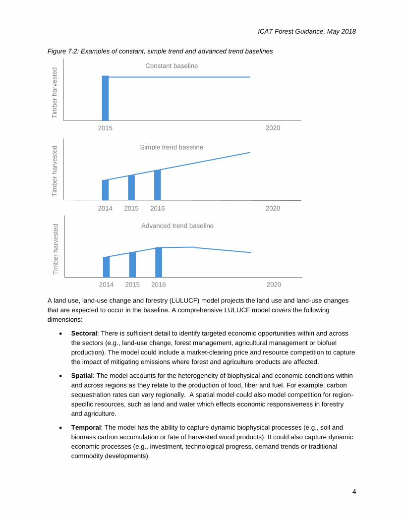
the baseline scenario. Figure 7.2 illustrates the different baseline approaches.
Constant baseline
This approach assumes there will be no change in land use, land cover or forest management practices
during the baseline period with respect to the situation prior to policy implementation. It represents the
simplest approach as only historical data is required. Either the most recent available data, or an average
ICAT Forest Guidance, May 2018
3
of the data from at least three years prior to the start of the policy implementation, can be used to quantify
the baseline parameters. This approach then assumes the parameters are held constant for the
assessment period and the baseline is the continuation of the current or historical situation. For example,
land will remain degraded under the baseline scenario. This baseline approach is the easiest to estimate,
however assessments based on a constant baseline may be less accurate.
Simple trend baseline
This baseline scenario approach assumes that land use, land cover and forest management practices will
evolve in the same way as they have in the past. This approach typically uses a linear or exponential
extrapolation of the historical trend for each baseline parameter. Users can employ a statistical regression
analysis to estimate trends. This approach can be easy to implement but it does not include any
assumptions about future policy measures or future mitigation actions. This approach should use
historical data from 5 to 10 years prior to the implementation of the policy. More data points will
strengthen the regression analysis. For example, land-use change in the future can be estimated by
assuming that the same rate change prior to policy implementation continues in the baseline.
Advanced trend baseline
This approach models the future evolution of the key drivers of emissions and factors in the impact of
many interacting elements, including trends in macroeconomic conditions, demographics and other non-
policy drivers.
A modeled baseline can be top-down or bottom-up:
Top-down model: This models how the economy or other exogenous factors (e.g.,
macroeconomic and demographic conditions) will impact the forestry sector. For example, the
approach may model how population growth will impact land use and then uses population
forecasts to predict baseline land-use change.
Bottom-up model: This approach models the interaction of key drivers on specific land use,
land-use change and forest management practices. It can offer a more detailed projection of
specific GHG sources and carbon pools. This approach will likely require detailed data such as
forest inventory, drivers of land-use change or specific timber or forest management practices. It
is suitable in countries where emissions from this sector are small or where their economic output
is modest, because the expected trends in macroeconomic and demographic conditions may not
be a good indicator of land use or land-use change.
ICAT Forest Guidance, May 2018
4
Figure 7.2: Examples of constant, simple trend and advanced trend baselines
A land use, land-use change and forestry (LULUCF) model projects the land use and land-use changes
that are expected to occur in the baseline. A comprehensive LULUCF model covers the following
dimensions:
Sectoral: There is sufficient detail to identify targeted economic opportunities within and across
the sectors (e.g., land-use change, forest management, agricultural management or biofuel
production). The model could include a market-clearing price and resource competition to capture
the impact of mitigating emissions where forest and agriculture products are affected.
Spatial: The model accounts for the heterogeneity of biophysical and economic conditions within
and across regions as they relate to the production of food, fiber and fuel. For example, carbon
sequestration rates can vary regionally. A spatial model could also model competition for region-
specific resources, such as land and water which effects economic responsiveness in forestry
and agriculture.
Temporal: The model has the ability to capture dynamic biophysical processes (e.g., soil and
biomass carbon accumulation or fate of harvested wood products). It could also capture dynamic
economic processes (e.g., investment, technological progress, demand trends or traditional
commodity developments).
2014 2020
Tim
ber
harv
este
d
2015 2016
Simple trend baseline
2015 2020
Tim
ber
harv
este
d Constant baseline
2014 2020
Tim
ber
harv
este
d
2015 2016
Advanced trend baseline
ICAT Forest Guidance, May 2018
5
LULUCF models can be categorised according to their functional and methodological aspects, as follows:
Statistical or econometric
Spatial interaction models
Optimisation models (which include linear, dynamic, hierarchical and non-linear programmes,
such as utility maximisation models and multi-criteria decision-making models)
Integrated models (gravity, simulation and entry-exit models)
Models based on natural sciences
Models based on GIS
Models based on the Markov Chain (MAPS, 2015)
There are a number of existing models which can be used to project an advanced trend baseline. For
example, the Global Biosphere Management Model (GLOBIOM) is an economic partial equilibrium model
of the competition for global land use. In GLOBIOM, the demand for land is modeled based on
exogenously specified regional drivers (including gross domestic product (GDP) growth, population
growth, evolution of food diets and global bioenergy demand), and local characteristics of the land. Brazil
has considered a model that includes the dynamics of land use that will be affected by competition and
scale. It provides the results of land allocation to different regions and biomasses in the country, thereby
projecting the type of natural vegetation that is converted (deforested) into agricultural land. The
projections are based on country level plans up to 2030 (MAPS, 2015).
7.1.2 Data Sources
Multiple types of data can be used to develop baseline scenarios, including top-down and bottom-up:
Top-down data: Macro-level data or statistics collected at the jurisdictional or sectoral level.
Examples include economic data on milk or meat consumption, land use maps, population and
GDP. In some cases, top-down data are aggregated from bottom-up data sources.
Bottom-up data: Data that are measured, monitored or collected at the facility, entity or project
level. Examples include agricultural or livestock census data on current and/or historical livestock
population, species, feed intake or land-use categories classified by climate region, soil type and
management.
The key parameters for estimating baseline emissions and removals in forests are:
Activity data: Hectares of forest land remaining forest land, non-forest land converted to forest
land, forest land converted to non-forest land.
Carbon stock change factor: The net change in carbon stocks per hectare of land, which can
also be expressed as CO2 emissions and removals per hectare of land. The carbon stock change
represents the emission factor for a land use or land management.
Existing data that has been collected for other assessments (including from national GHG inventories,
National Communications and Biennial Update Reports), which are prepared following IPCC guidelines,
can be used for determining the baseline scenario and estimating baseline emissions and removals.
ICAT Forest Guidance, May 2018
6
Where relevant, it may be important to use data that is consistent with national or sub-national level
sectoral baselines. Sources of data for the key parameters include:
Forest Cover maps and regionally specific data
Country-level data from NAMA and low carbon development programmes
Country-level REDD+ reporting or studies (e.g., national or subnational REDD+ forest reference
emission levels (FRELs) or forest reference levels (FRLs))
Global Forest Watch (GFW)1, US Geological Survey (USGS)2, FAO databases3
7.1.3 Choosing the approach to determine the baseline scenario
The choice of approach to determine the baseline scenario depends on users’ resources, capacity,
access to data, availability of models and methodologies, and the parameters that are expected to
change. A constant baseline is the simplest option and may be appropriate when parameters are
considered likely to remain stable over time. A simple trend baseline is most appropriate if the change in
baseline parameter values is expected to remain stable over time. Advanced trend baseline approaches
may yield more accurate results than other approaches, since they take into account various drivers that
affect conditions over time. However, more complex baselines will only be more accurate if the underlying
data and methods used to model the impacts of drivers are robust. Users should use methods and data
that yield the most accurate results within a given context, based on the resources and data available.
Estimate baseline emissions
This section provides guidance on estimating baseline emissions. It provides suggestions for identifying
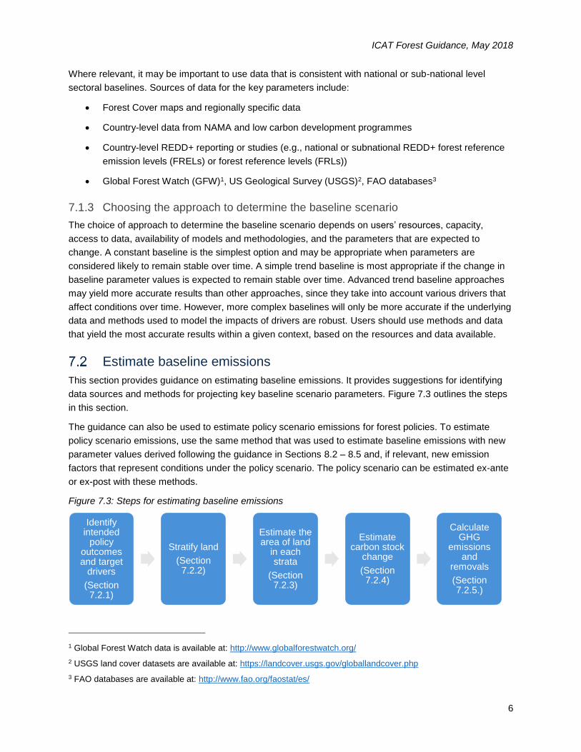
data sources and methods for projecting key baseline scenario parameters. Figure 7.3 outlines the steps
in this section.
The guidance can also be used to estimate policy scenario emissions for forest policies. To estimate
policy scenario emissions, use the same method that was used to estimate baseline emissions with new
parameter values derived following the guidance in Sections 8.2 – 8.5 and, if relevant, new emission
factors that represent conditions under the policy scenario. The policy scenario can be estimated ex-ante
or ex-post with these methods.
Figure 7.3: Steps for estimating baseline emissions
1 Global Forest Watch data is available at: http://www.globalforestwatch.org/
2 USGS land cover datasets are available at: https://landcover.usgs.gov/globallandcover.php
3 FAO databases are available at: http://www.fao.org/faostat/es/
Identify intended
policy outcomes and target
drivers
(Section 7.2.1)
Stratify land
(Section 7.2.2)
Estimate the area of land
in each strata
(Section 7.2.3)
Estimate carbon stock
change
(Section 7.2.4)
Calculate GHG
emissions and
removals
(Section 7.2.5.)
ICAT Forest Guidance, May 2018
7
Changes in land use can lead to an increase or decrease in forest carbon. For example, conversion of
cropland to forest land results in a net increase of forest carbon. Conversely, cropland converted to
forests land (deforestation) results in net losses of forest carbon. Where land use remains the same over
time (e.g., forest land remaining forest land), changes in management (e.g., increasing the minimum age
of cutting thresholds) can result in net increases or decreases in forest carbon. Policy impacts on forest
carbon are estimated in terms of how the policy changes land use and management.
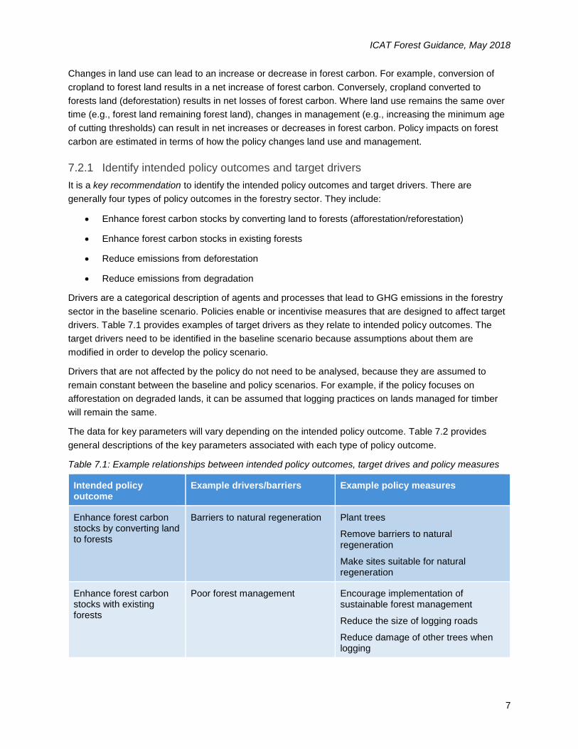
7.2.1 Identify intended policy outcomes and target drivers
It is a key recommendation to identify the intended policy outcomes and target drivers. There are
generally four types of policy outcomes in the forestry sector. They include:
Enhance forest carbon stocks by converting land to forests (afforestation/reforestation)
Enhance forest carbon stocks in existing forests
Reduce emissions from deforestation
Reduce emissions from degradation
Drivers are a categorical description of agents and processes that lead to GHG emissions in the forestry
sector in the baseline scenario. Policies enable or incentivise measures that are designed to affect target
drivers. Table 7.1 provides examples of target drivers as they relate to intended policy outcomes. The
target drivers need to be identified in the baseline scenario because assumptions about them are
modified in order to develop the policy scenario.
Drivers that are not affected by the policy do not need to be analysed, because they are assumed to
remain constant between the baseline and policy scenarios. For example, if the policy focuses on
afforestation on degraded lands, it can be assumed that logging practices on lands managed for timber
will remain the same.
The data for key parameters will vary depending on the intended policy outcome. Table 7.2 provides
general descriptions of the key parameters associated with each type of policy outcome.
Table 7.1: Example relationships between intended policy outcomes, target drives and policy measures
Intended policy outcome
Example drivers/barriers Example policy measures
Enhance forest carbon stocks by converting land to forests
Barriers to natural regeneration Plant trees
Remove barriers to natural regeneration
Make sites suitable for natural regeneration
Enhance forest carbon stocks with existing forests
Poor forest management Encourage implementation of sustainable forest management
Reduce the size of logging roads
Reduce damage of other trees when logging
ICAT Forest Guidance, May 2018
8
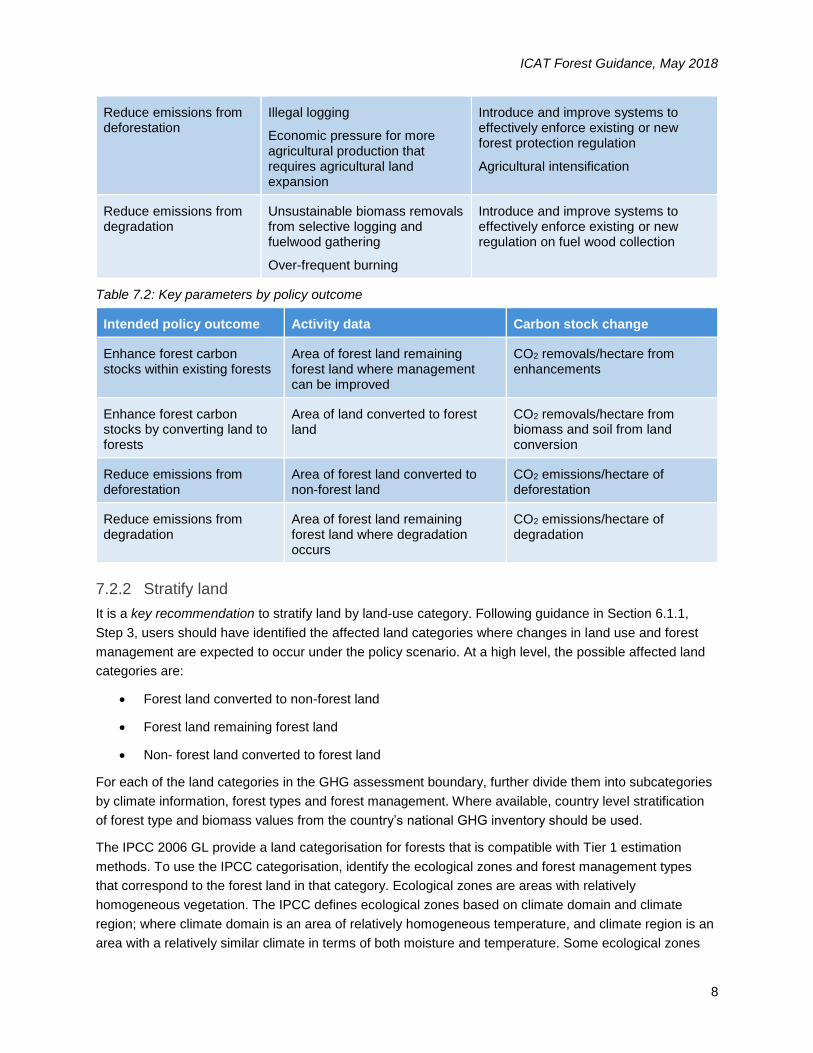
Reduce emissions from deforestation
Illegal logging
Economic pressure for more agricultural production that requires agricultural land expansion
Introduce and improve systems to effectively enforce existing or new forest protection regulation
Agricultural intensification
Reduce emissions from degradation
Unsustainable biomass removals from selective logging and fuelwood gathering
Over-frequent burning
Introduce and improve systems to effectively enforce existing or new regulation on fuel wood collection
Table 7.2: Key parameters by policy outcome
Intended policy outcome Activity data Carbon stock change
Enhance forest carbon stocks within existing forests
Area of forest land remaining forest land where management can be improved
CO2 removals/hectare from enhancements
Enhance forest carbon stocks by converting land to forests
Area of land converted to forest land
CO2 removals/hectare from biomass and soil from land conversion
Reduce emissions from deforestation
Area of forest land converted to non-forest land
CO2 emissions/hectare of deforestation
Reduce emissions from degradation
Area of forest land remaining forest land where degradation occurs
CO2 emissions/hectare of degradation
7.2.2 Stratify land
It is a key recommendation to stratify land by land-use category. Following guidance in Section 6.1.1,
Step 3, users should have identified the affected land categories where changes in land use and forest
management are expected to occur under the policy scenario. At a high level, the possible affected land
categories are:
Forest land converted to non-forest land
Forest land remaining forest land
Non- forest land converted to forest land
For each of the land categories in the GHG assessment boundary, further divide them into subcategories
by climate information, forest types and forest management. Where available, country level stratification
of forest type and biomass values from the country’s national GHG inventory should be used.
The IPCC 2006 GL provide a land categorisation for forests that is compatible with Tier 1 estimation
methods. To use the IPCC categorisation, identify the ecological zones and forest management types
that correspond to the forest land in that category. Ecological zones are areas with relatively
homogeneous vegetation. The IPCC defines ecological zones based on climate domain and climate
region; where climate domain is an area of relatively homogeneous temperature, and climate region is an
area with a relatively similar climate in terms of both moisture and temperature. Some ecological zones
ICAT Forest Guidance, May 2018
9
are, for example: tropical rain forest, subtropical humid forest, temperate oceanic forest and boreal
coniferous forest. IPCC definitions of ecological zones according to climate domain and climate region
are provided in Table 4.1 of the IPCC 2006 GL, Volume 4, Chapter 4.
Within each ecological zone, further define subcategories of forest land in terms of how the forests are
managed. The IPCC provides two categories for this: natural and plantation forest. Natural forests are
generally naturally re-growing stands with reduced or minimum human intervention. Plantation forests are
intensively managed (including planted, managed, harvested and replanted). The IPCC provides Tier 1
estimated biomass values for natural and plantation forests for all ecological zones (Table 4.12 of the
IPCC 2006 GL, Volume 4, Chapter 4). Use the IPCC biomass values and information about forest
management and forest biomass in your country to develop criteria for classifying forests into natural and
plantation and document the criteria you have used.
The subcategories outlined above (i.e., ecological zone and management type), are recommended
because they are compatible with using IPCC Tier 1 emission factors for estimating the carbon in forest
biomass. The land categorisation can be done differently where Tier 2 emission factors are available or a
derived Tier 2 estimate of CO2 emissions/removals for each land category can be calculated. Where the
policy aims to reduce forest degradation, higher approaches and tiers should be used to capture
changes. Higher approach and tier methods require more data, but can yield a more accurate GHG
impacts assessment. Users should consider the objectives of the policy when selecting which method to
use.
7.2.3 Estimate the area of land in each stratum
It is a key recommendation to estimate the area of land in each stratum. Land area can be derived from
national data sources that are widely accepted among policymakers and endorsed by the government.
Potential data sources include remote sensed and aerial imagery, ministry of agriculture or forests,
national agricultural or forest research institutes, and international agencies (e.g., FAO). Relevant land
area data compiled for the national GHG inventory is also a relevant data source. These data sources will
typically provide information on historical and current land area.
There are several resources that detail how to develop land area estimates for forest carbon monitoring:
IPCC 2003 Good Practice Guidelines for Land Use, Land-Use Change and Forestry4
IPCC 2006 GL for AFOLU, Volume 45
Global Observation of Forest Cover and Land Dynamics (GOFC GOLD) Sourcebook6
Winrock Standard Operating Procedures for Terrestrial Carbon Measurement 20167
Global Forest Observation Initiative methods and guidance documentation8
4 Available at: http://www.ipcc-nggip.iges.or.jp/public/gpglulucf/gpglulucf.html
5 Available at: http://www.ipcc-nggip.iges.or.jp/public/2006gl/vol4.html
6 Available at: http://www.gofcgold.wur.nl/redd/
7 Available at: http://www.leafasia.org/tools/winrock-standard-operating-procedures-terrestrial-carbon-measurementfield-sop-manual
8 Available at: http://www.gfoi.org/methods-guidance/
ICAT Forest Guidance, May 2018
10
These resources can be used to estimate a time series of land area for the baseline assessment. The
time series is the number or hectares of land in each land stratum each year of the assessment period.
Any of the approaches discussed in Section 7.1 can be used to project the hectares of land over time
based on current and historical data.
7.2.4 Estimate carbon stock change
It is a key recommendation to estimate the carbon stock change (i.e., emission factor) for each carbon
pool in each land stratum. At a minimum, the carbon stock change for the living aboveground and
belowground biomass (living biomass) pool should be estimated. For afforestation/reforestation and
reduced deforestation activities, carbon stock change for dead organic matter and soil carbon pools can
also be estimated where these pools are included in the GHG assessment boundary.
When deciding which pools to estimate the carbon stock change for, users may encounter trade-offs
between the principle of accuracy and the cost of collecting data. Conservativeness can serve as a
moderator to accuracy in order to balance costs while maintaining the credibility the GHG estimate. Users
can rely on existing data and methods for estimating carbon stock change including the following:
National forest inventories
Subnational or regional forest inventory datasets
Independent relevant or regional scientific studies or datasets
Values published in scientific literature
Values provided in the IPCC 2006 GL
The guidance below is for estimating carbon stock change based on the living biomass carbon pool only.
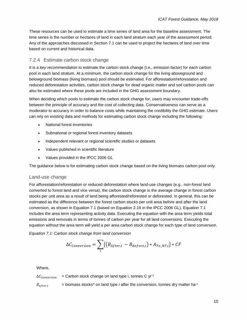
Land-use change
For afforestation/reforestation or reduced deforestation where land-use changes (e.g., non-forest land
converted to forest land and vice versa), the carbon stock change is the average change in forest carbon
stocks per unit area as a result of land being afforested/reforested or deforested. In general, this can be
estimated as the difference between the forest carbon stocks per unit area before and after the land
conversion, as shown in Equation 7.1 (based on Equation 2.16 in the IPCC 2006 GL). Equation 7.1
includes the area term representing activity data. Executing the equation with the area term yields total
emissions and removals in terms of tonnes of carbon per year for all land conversions. Executing the
equation without the area term will yield a per area carbon stock change for each type of land conversion.
Equation 7.1: Carbon stock change from land conversion
∆𝐶𝐶𝑜𝑛𝑣𝑒𝑟𝑠𝑖𝑜𝑛 = ∑{(𝐵𝐴𝑓𝑡𝑒𝑟,𝑖 − 𝐵𝐵𝑒𝑓𝑜𝑟𝑒,𝑖) ∗ 𝐴𝑇𝑜_𝑁𝐹,𝑖} ∗ 𝐶𝐹
𝑖
Where,
∆𝐶𝐶𝑜𝑛𝑣𝑒𝑟𝑠𝑖𝑜𝑛 = Carbon stock change on land type i, tonnes C yr-1
𝐵𝐴𝑓𝑡𝑒𝑟,𝑖 = biomass stocks* on land type i after the conversion, tonnes dry matter ha-1
ICAT Forest Guidance, May 2018
11
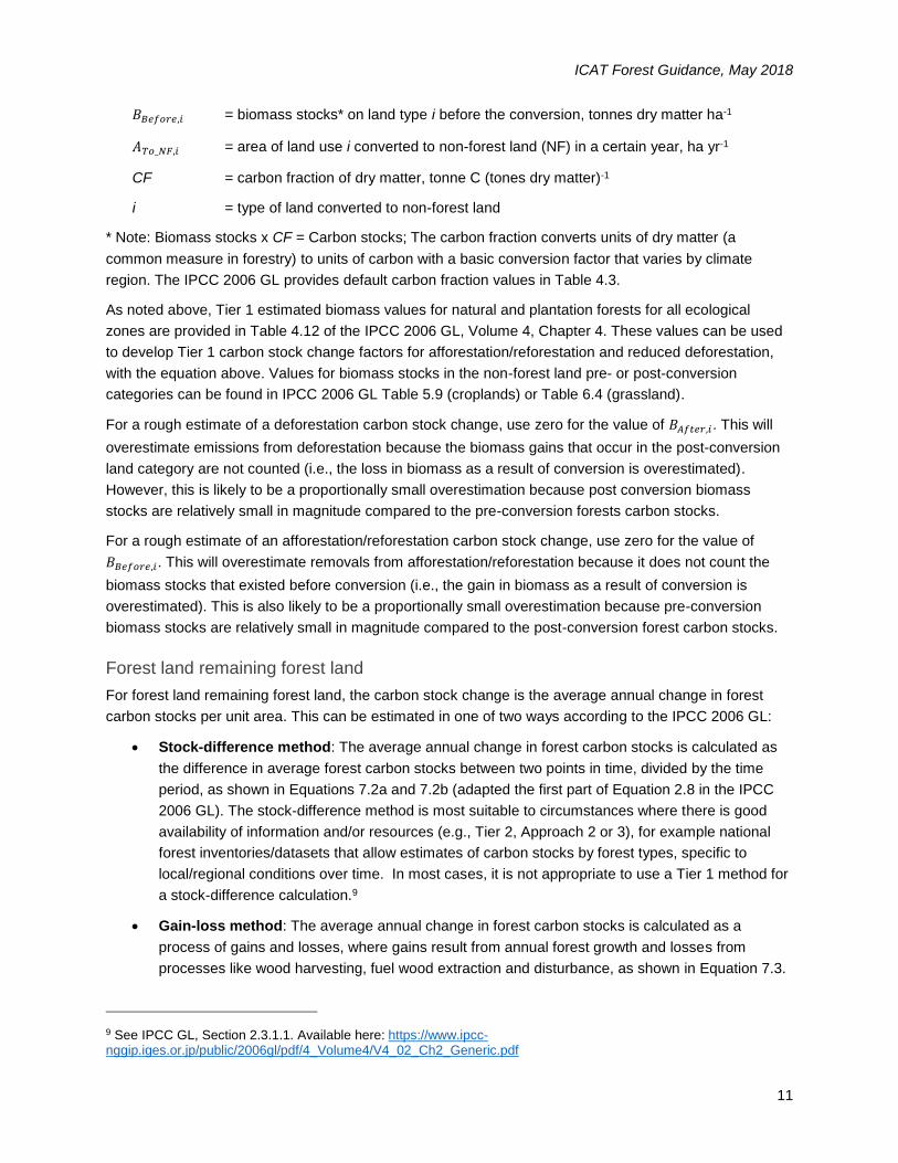
𝐵𝐵𝑒𝑓𝑜𝑟𝑒,𝑖 = biomass stocks* on land type i before the conversion, tonnes dry matter ha-1
𝐴𝑇𝑜_𝑁𝐹,𝑖 = area of land use i converted to non-forest land (NF) in a certain year, ha yr-1
CF = carbon fraction of dry matter, tonne C (tones dry matter)-1
i = type of land converted to non-forest land
* Note: Biomass stocks x CF = Carbon stocks; The carbon fraction converts units of dry matter (a
common measure in forestry) to units of carbon with a basic conversion factor that varies by climate
region. The IPCC 2006 GL provides default carbon fraction values in Table 4.3.
As noted above, Tier 1 estimated biomass values for natural and plantation forests for all ecological
zones are provided in Table 4.12 of the IPCC 2006 GL, Volume 4, Chapter 4. These values can be used
to develop Tier 1 carbon stock change factors for afforestation/reforestation and reduced deforestation,
with the equation above. Values for biomass stocks in the non-forest land pre- or post-conversion
categories can be found in IPCC 2006 GL Table 5.9 (croplands) or Table 6.4 (grassland).
For a rough estimate of a deforestation carbon stock change, use zero for the value of 𝐵𝐴𝑓𝑡𝑒𝑟,𝑖. This will
overestimate emissions from deforestation because the biomass gains that occur in the post-conversion
land category are not counted (i.e., the loss in biomass as a result of conversion is overestimated).
However, this is likely to be a proportionally small overestimation because post conversion biomass
stocks are relatively small in magnitude compared to the pre-conversion forests carbon stocks.
For a rough estimate of an afforestation/reforestation carbon stock change, use zero for the value of
𝐵𝐵𝑒𝑓𝑜𝑟𝑒,𝑖. This will overestimate removals from afforestation/reforestation because it does not count the
biomass stocks that existed before conversion (i.e., the gain in biomass as a result of conversion is
overestimated). This is also likely to be a proportionally small overestimation because pre-conversion
biomass stocks are relatively small in magnitude compared to the post-conversion forest carbon stocks.
Forest land remaining forest land
For forest land remaining forest land, the carbon stock change is the average annual change in forest
carbon stocks per unit area. This can be estimated in one of two ways according to the IPCC 2006 GL:
Stock-difference method: The average annual change in forest carbon stocks is calculated as
the difference in average forest carbon stocks between two points in time, divided by the time
period, as shown in Equations 7.2a and 7.2b (adapted the first part of Equation 2.8 in the IPCC
2006 GL). The stock-difference method is most suitable to circumstances where there is good
availability of information and/or resources (e.g., Tier 2, Approach 2 or 3), for example national
forest inventories/datasets that allow estimates of carbon stocks by forest types, specific to
local/regional conditions over time. In most cases, it is not appropriate to use a Tier 1 method for
a stock-difference calculation.9
Gain-loss method: The average annual change in forest carbon stocks is calculated as a
process of gains and losses, where gains result from annual forest growth and losses from
processes like wood harvesting, fuel wood extraction and disturbance, as shown in Equation 7.3.
9 See IPCC GL, Section 2.3.1.1. Available here: https://www.ipcc-nggip.iges.or.jp/public/2006gl/pdf/4_Volume4/V4_02_Ch2_Generic.pdf
ICAT Forest Guidance, May 2018
12
The gain-loss method is most suitable for circumstances when countries do not have time series
information on activity data and emission factors to assess by stock-difference method.
Both the stock-difference and gain-loss methods are executed with the area term (activity data) in the
equations, which yields total change in carbon stocks for all land strata in forest land remaining forest
land. Therefore the carbon stock change is embedded in the quantification of total emissions and
removals.
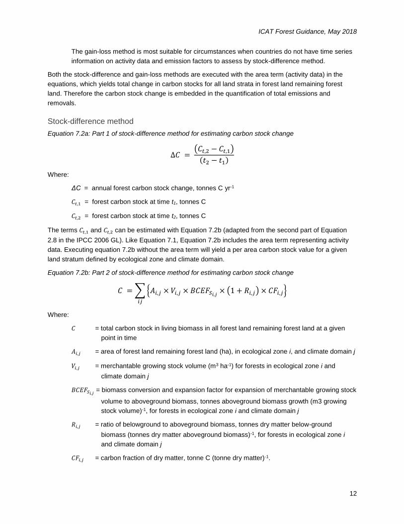
Stock-difference method
Equation 7.2a: Part 1 of stock-difference method for estimating carbon stock change
∆𝐶 = (𝐶𝑡,2 − 𝐶𝑡,1)
(𝑡2 − 𝑡1)
Where:
ΔC = annual forest carbon stock change, tonnes C yr-1
𝐶𝑡,1 = forest carbon stock at time t1, tonnes C
𝐶𝑡,2 = forest carbon stock at time t2, tonnes C
The terms 𝐶𝑡,1 and 𝐶𝑡,2 can be estimated with Equation 7.2b (adapted from the second part of Equation
2.8 in the IPCC 2006 GL). Like Equation 7.1, Equation 7.2b includes the area term representing activity
data. Executing equation 7.2b without the area term will yield a per area carbon stock value for a given
land stratum defined by ecological zone and climate domain.
Equation 7.2b: Part 2 of stock-difference method for estimating carbon stock change
𝐶 = ∑ {𝐴𝑖,𝑗 × 𝑉𝑖,𝑗 × 𝐵𝐶𝐸𝐹𝑆𝑖,𝑗× (1 + 𝑅𝑖,𝑗) × 𝐶𝐹𝑖,𝑗}
𝑖𝑗
Where:
𝐶 = total carbon stock in living biomass in all forest land remaining forest land at a given
point in time
𝐴𝑖,𝑗 = area of forest land remaining forest land (ha), in ecological zone i, and climate domain j
𝑉𝑖,𝑗 = merchantable growing stock volume (m3 ha-1) for forests in ecological zone i and
climate domain j
𝐵𝐶𝐸𝐹𝑆𝑖,𝑗 = biomass conversion and expansion factor for expansion of merchantable growing stock
volume to aboveground biomass, tonnes aboveground biomass growth (m3 growing
stock volume)-1, for forests in ecological zone i and climate domain j
𝑅𝑖,𝑗 = ratio of belowground to aboveground biomass, tonnes dry matter below-ground
biomass (tonnes dry matter aboveground biomass)-1, for forests in ecological zone i
and climate domain j
𝐶𝐹𝑖,𝑗 = carbon fraction of dry matter, tonne C (tonne dry matter)-1.
ICAT Forest Guidance, May 2018
13
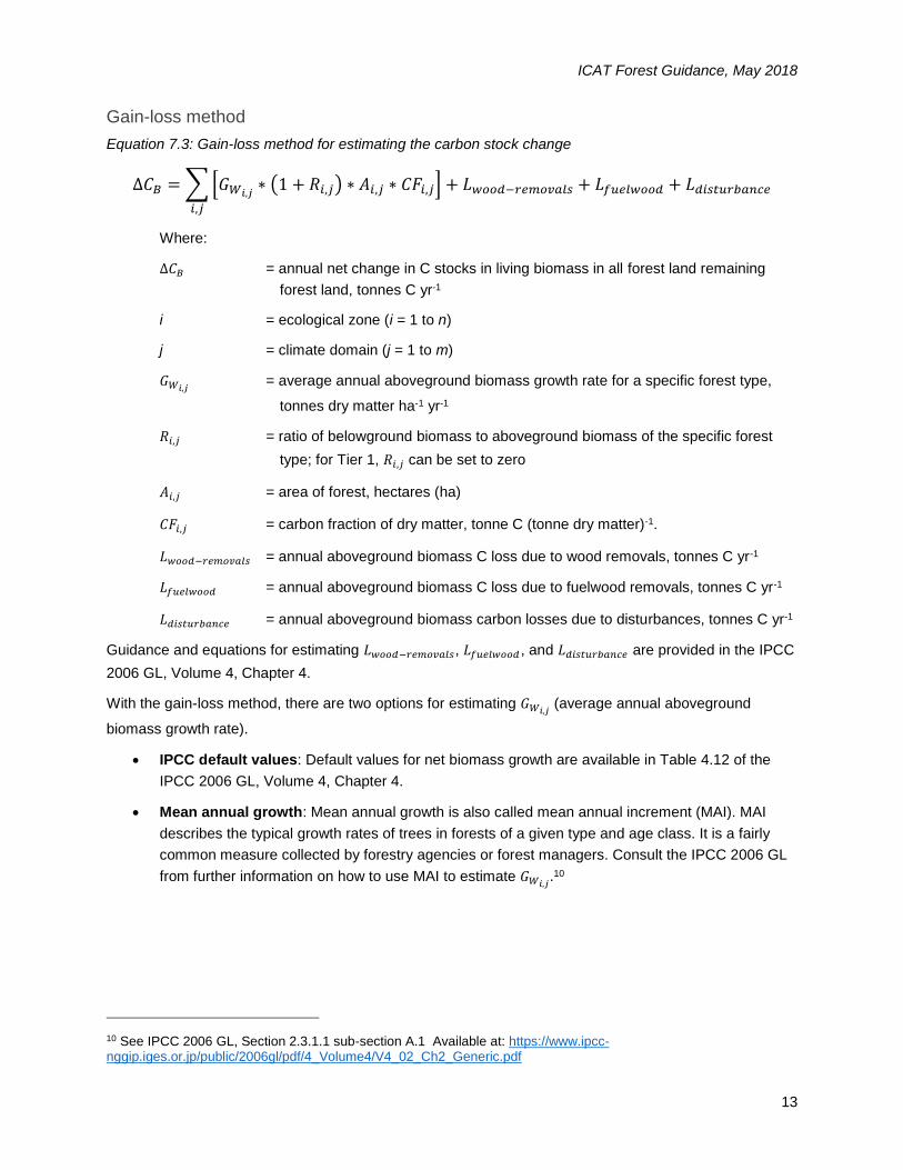
Gain-loss method
Equation 7.3: Gain-loss method for estimating the carbon stock change
∆𝐶𝐵 = ∑ [𝐺𝑊𝑖,𝑗∗ (1 + 𝑅𝑖,𝑗) ∗ 𝐴𝑖,𝑗 ∗ 𝐶𝐹𝑖,𝑗] + 𝐿𝑤𝑜𝑜𝑑−𝑟𝑒𝑚𝑜𝑣𝑎𝑙𝑠 + 𝐿𝑓𝑢𝑒𝑙𝑤𝑜𝑜𝑑 + 𝐿𝑑𝑖𝑠𝑡𝑢𝑟𝑏𝑎𝑛𝑐𝑒
𝑖,𝑗
Where:
∆𝐶𝐵 = annual net change in C stocks in living biomass in all forest land remaining
forest land, tonnes C yr-1
i = ecological zone (i = 1 to n)
j = climate domain (j = 1 to m)
𝐺𝑊𝑖,𝑗 = average annual aboveground biomass growth rate for a specific forest type,
tonnes dry matter ha-1 yr-1
𝑅𝑖,𝑗 = ratio of belowground biomass to aboveground biomass of the specific forest
type; for Tier 1, 𝑅𝑖,𝑗 can be set to zero
𝐴𝑖,𝑗 = area of forest, hectares (ha)
𝐶𝐹𝑖,𝑗 = carbon fraction of dry matter, tonne C (tonne dry matter)-1.
𝐿𝑤𝑜𝑜𝑑−𝑟𝑒𝑚𝑜𝑣𝑎𝑙𝑠 = annual aboveground biomass C loss due to wood removals, tonnes C yr-1
𝐿𝑓𝑢𝑒𝑙𝑤𝑜𝑜𝑑 = annual aboveground biomass C loss due to fuelwood removals, tonnes C yr-1
𝐿𝑑𝑖𝑠𝑡𝑢𝑟𝑏𝑎𝑛𝑐𝑒 = annual aboveground biomass carbon losses due to disturbances, tonnes C yr-1
Guidance and equations for estimating 𝐿𝑤𝑜𝑜𝑑−𝑟𝑒𝑚𝑜𝑣𝑎𝑙𝑠, 𝐿𝑓𝑢𝑒𝑙𝑤𝑜𝑜𝑑 , and 𝐿𝑑𝑖𝑠𝑡𝑢𝑟𝑏𝑎𝑛𝑐𝑒 are provided in the IPCC
2006 GL, Volume 4, Chapter 4.
With the gain-loss method, there are two options for estimating 𝐺𝑊𝑖,𝑗 (average annual aboveground
biomass growth rate).
IPCC default values: Default values for net biomass growth are available in Table 4.12 of the
IPCC 2006 GL, Volume 4, Chapter 4.
Mean annual growth: Mean annual growth is also called mean annual increment (MAI). MAI
describes the typical growth rates of trees in forests of a given type and age class. It is a fairly
common measure collected by forestry agencies or forest managers. Consult the IPCC 2006 GL
from further information on how to use MAI to estimate 𝐺𝑊𝑖,𝑗.10
10 See IPCC 2006 GL, Section 2.3.1.1 sub-section A.1 Available at: https://www.ipcc-nggip.iges.or.jp/public/2006gl/pdf/4_Volume4/V4_02_Ch2_Generic.pdf
ICAT Forest Guidance, May 2018
14
Further resources
Comprehensive guidance on estimating forest carbon stock changes in all carbon pools can be found in
numerous resources.
IPCC 2003 Good Practice Guidelines for Land Use, Land-Use Change and Forestry
IPCC 2006 GL for AFOLU, Volume 4
Global Observation of Forest Cover and Land Dynamics (GOFC GOLD) Sourcebook
Winrock Standard Operating Procedures for Terrestrial Carbon Measurement 2016
Global Forest Observation Initiative (GFOI) Methods and Guidance Documentation
The GOFC GOLD Sourcebook and GFOI Methods and Guidance Documentation are particularly relevant
resources for estimating carbon stock change for multiple carbon pools for enhancing carbon stocks
through afforestation/reforestation, enhancing carbon stocks through management, deforestation, and
degradation. Where existing higher-tier data is available (including emission factors, biomass values or
land stratification), such data can be used to increase accuracy and completeness of the estimate.
7.2.5 Calculate GHG emissions and removals
It is a key recommendation to calculate the cumulative GHG emissions and removals for the baseline
scenario over the assessment period. Estimate annual carbon stock change for each land stratum each
year in the baseline scenario using area data and carbon stock change equations provided above for
land-use change (afforestation/reforestation and reduced deforestation) and forest land remaining forest
land. Sum annual carbon stock change by stratum across all land strata to yield net annual carbon stock
change on lands in the GHG assessment boundary.
Finally, sum the annual carbon stock changes for all years in the assessment period to yield cumulative
carbon stock change in the baseline scenario. Convert the cumulative carbon stock change to GHG
emissions expressed as tonnes of CO2e by multiplying the cumulative carbon stock change by 44/12 and
by -1. This yields total cumulative CO2e emissions (positive) or removals (negative) for the baseline.
ICAT Forest Guidance, May 2018
15
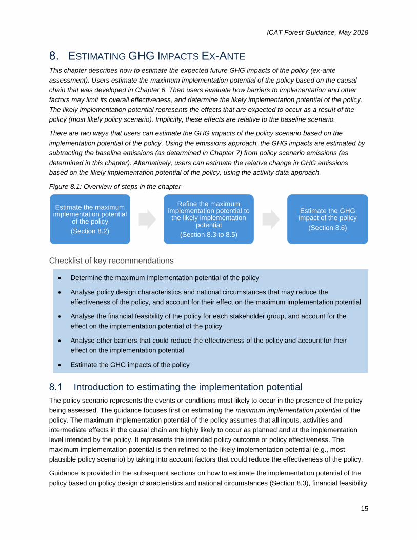
ESTIMATING GHG IMPACTS EX-ANTE This chapter describes how to estimate the expected future GHG impacts of the policy (ex-ante
assessment). Users estimate the maximum implementation potential of the policy based on the causal
chain that was developed in Chapter 6. Then users evaluate how barriers to implementation and other
factors may limit its overall effectiveness, and determine the likely implementation potential of the policy.
The likely implementation potential represents the effects that are expected to occur as a result of the
policy (most likely policy scenario). Implicitly, these effects are relative to the baseline scenario.
There are two ways that users can estimate the GHG impacts of the policy scenario based on the
implementation potential of the policy. Using the emissions approach, the GHG impacts are estimated by
subtracting the baseline emissions (as determined in Chapter 7) from policy scenario emissions (as
determined in this chapter). Alternatively, users can estimate the relative change in GHG emissions
based on the likely implementation potential of the policy, using the activity data approach.
Figure 8.1: Overview of steps in the chapter
Checklist of key recommendations
Determine the maximum implementation potential of the policy
Analyse policy design characteristics and national circumstances that may reduce the
effectiveness of the policy, and account for their effect on the maximum implementation potential
Analyse the financial feasibility of the policy for each stakeholder group, and account for the
effect on the implementation potential of the policy
Analyse other barriers that could reduce the effectiveness of the policy and account for their
effect on the implementation potential
Estimate the GHG impacts of the policy
Introduction to estimating the implementation potential
The policy scenario represents the events or conditions most likely to occur in the presence of the policy
being assessed. The guidance focuses first on estimating the maximum implementation potential of the
policy. The maximum implementation potential of the policy assumes that all inputs, activities and
intermediate effects in the causal chain are highly likely to occur as planned and at the implementation
level intended by the policy. It represents the intended policy outcome or policy effectiveness. The
maximum implementation potential is then refined to the likely implementation potential (e.g., most
plausible policy scenario) by taking into account factors that could reduce the effectiveness of the policy.
Guidance is provided in the subsequent sections on how to estimate the implementation potential of the
policy based on policy design characteristics and national circumstances (Section 8.3), financial feasibility
Estimate the maximum implementation potential
of the policy
(Section 8.2)
Refine the maximum implementation potential to the likely implementation
potential
(Section 8.3 to 8.5)
Estimate the GHG impact of the policy
(Section 8.6)
ICAT Forest Guidance, May 2018
16
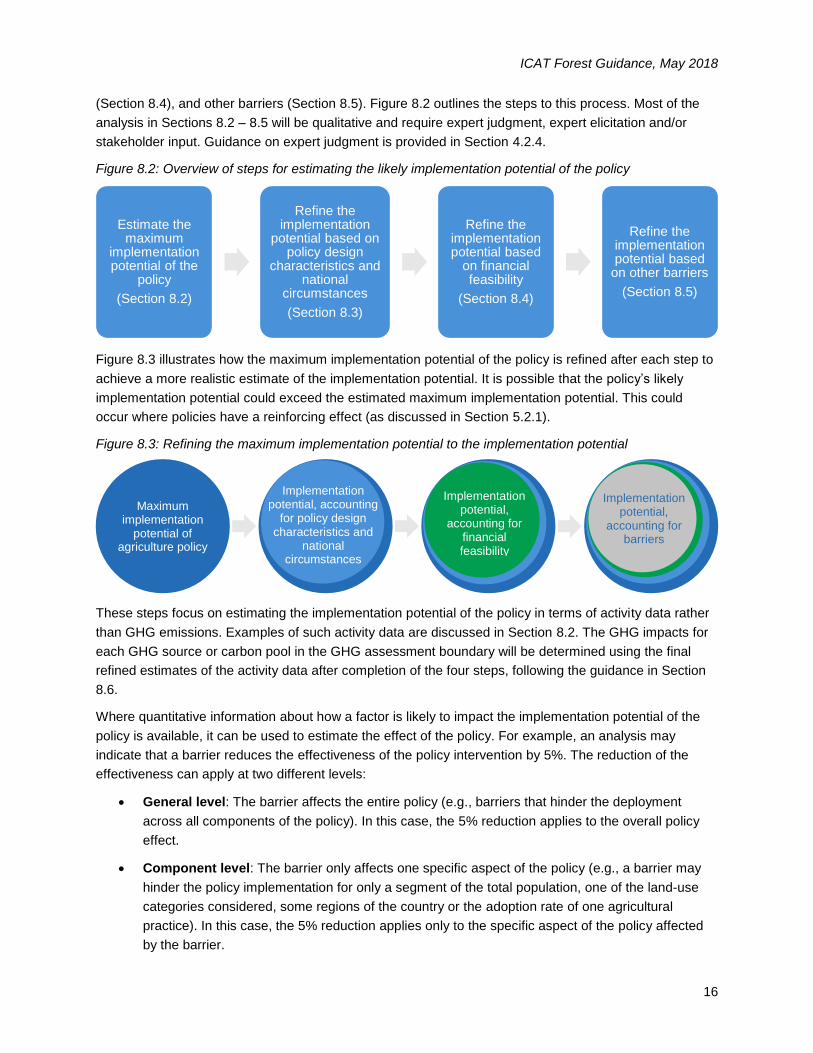
(Section 8.4), and other barriers (Section 8.5). Figure 8.2 outlines the steps to this process. Most of the
analysis in Sections 8.2 – 8.5 will be qualitative and require expert judgment, expert elicitation and/or
stakeholder input. Guidance on expert judgment is provided in Section 4.2.4.
Figure 8.2: Overview of steps for estimating the likely implementation potential of the policy
Figure 8.3 illustrates how the maximum implementation potential of the policy is refined after each step to
achieve a more realistic estimate of the implementation potential. It is possible that the policy’s likely
implementation potential could exceed the estimated maximum implementation potential. This could
occur where policies have a reinforcing effect (as discussed in Section 5.2.1).
Figure 8.3: Refining the maximum implementation potential to the implementation potential
These steps focus on estimating the implementation potential of the policy in terms of activity data rather
than GHG emissions. Examples of such activity data are discussed in Section 8.2. The GHG impacts for
each GHG source or carbon pool in the GHG assessment boundary will be determined using the final
refined estimates of the activity data after completion of the four steps, following the guidance in Section
8.6.
Where quantitative information about how a factor is likely to impact the implementation potential of the
policy is available, it can be used to estimate the effect of the policy. For example, an analysis may
indicate that a barrier reduces the effectiveness of the policy intervention by 5%. The reduction of the
effectiveness can apply at two different levels:
General level: The barrier affects the entire policy (e.g., barriers that hinder the deployment
across all components of the policy). In this case, the 5% reduction applies to the overall policy
effect.
Component level: The barrier only affects one specific aspect of the policy (e.g., a barrier may
hinder the policy implementation for only a segment of the total population, one of the land-use
categories considered, some regions of the country or the adoption rate of one agricultural
practice). In this case, the 5% reduction applies only to the specific aspect of the policy affected
by the barrier.
Estimate the maximum
implementation potential of the
policy
(Section 8.2)
Refine the implementation
potential based on policy design
characteristics and national
circumstances
(Section 8.3)
Refine the implementation potential based
on financial feasibility
(Section 8.4)
Refine the implementation potential based
on other barriers
(Section 8.5)
Implementation potential,
accounting for financial feasibility
Implementation potential, accounting
for policy design characteristics and
national circumstances
Implementation potential,
accounting for barriers
Maximum implementation
potential of agriculture policy
ICAT Forest Guidance, May 2018
17
To the extent possible, identify a single policy scenario that is considered to be the most likely. In certain
cases, multiple policy scenario options may seem equally plausible. Users can develop multiple policy
scenarios, each based on different sets of assumptions, rather than just one set. This approach produces
a range of possible emission reductions scenarios. Users can then conduct a sensitivity analysis to see
how the results vary depending on the selection of policy scenario options. More guidance about
conducting a sensitivity analysis is provided in Chapter 12 of the Policy and Action Standard.
An example is used to demonstrate how to estimate the implementation potential of a policy. A
description of the example is provided in Box 8.1. The implementation potential of the example policy is
assessed on the basis of the estimated number of hectares of land on which the policy will be
implemented.
Box 8.1: Example of forest policy for national or subnational level GHG mitigation
The government is considering the option of promoting sustainable forest management and
afforestation/reforestation through the introduction of a payment for ecosystem services (PES)
programme combined with a new tax legislated for users of ecosystem services. Government officials
are in the initial phase of the policy development process and need to consider all aspects relating to
legislating, designing and implementing the policy intervention. It is expected that the national
legislative body will enact a new tax for all users of ecosystem services (primarily for water and
hydroelectric utilities, but other sectors may be included such as tourism companies). The national
taxing agency will collect the tax, which will fund a new PES programme (estimated to be about 1-2%
annual revenue) to provide programme incentives, as well as administrative and operational expenses.
The goals for the PES programme are to 1) expand SFM activities and 2) promote A/R through tree
planting or natural regeneration.
Further details on the policy can be found in Section 5.1.
Determine the maximum implementation potential
It is a key recommendation to determine the maximum implementation potential of the policy. For each
GHG source or carbon pool in the GHG assessment boundary, choose a type of activity data to assess
the implementation potential of the policy. The type of activity data chosen should be a parameter that is
expected to change as a result of the policy (e.g., hectares of forest land prevented from being converted
to cropland), and be used to estimate GHG impacts. Therefore the activity data serves as a proxy for the
policy outcome. The maximum implementation potential is expressed in terms of activity data. Table 8.1
provides examples of the types of activity data to consider.
Table 8.1: Examples of types of activity data for analysing implementation potential
GHG source or carbon pool
Policy Activity Data
Biomass and soil carbon
Incentives for sustainable forest management
Payments for afforestation/reforestation
Hectares of forest land prevented from being converted to non-forest land
Hectares of forest land remaining forest land where management is improved

ICAT Forest Guidance, May 2018
18
Technical assistance to improve management
Introducing and improving systems to effectively enforce existing or new environmental regulation
Hectares of forest land remaining forest land where sustainable forest management is implemented
Hectares of cropland converted to forest land
Hectares of grassland converted to forest land
The maximum implementation potential can be estimated based on a number of elements. The options
include using a mitigation goal, expected adoption of practices or technologies, financial considerations,
land area and other resource potential, and expert judgment. Each element is further explained below.
The maximum implementation potential can be estimated using a single element or a combination of
elements. A combination will likely yield a better estimate.
8.2.1 Mitigation goal
When there is an intended level of mitigation and/or an explicit goal for the policy, the goal along with
other details of the policy can be used to estimate the maximum implementation potential. A mitigation
goal may include, among other things, the target amount of emission reductions to be reduced or carbon
stocks enhanced as a result of the policy, the targeted amount of land area or adoption rate, or the total
expected emission reductions and removals from a specific GHG source or carbon pool. The mitigation
goal may not be in the same units as the activity data, and additional information from surveys and
national statistics may be needed to estimate how the goal will translate into actions or land areas. For
example, an explicit goal for a forest policy could be to increase the minimum diameter cutting threshold
on all publicly managed timber forests by 2020.
Using a stated goal as the main indication of intended policy outcomes or policy effectiveness can be
highly uncertain. At a minimum, the mitigation goal needs to be specific enough to reflect an intended
level of mitigation.
8.2.2 Adoption of practices or technologies
The expected level of adoption of the practice or technology that is targeted by the policy can be used to
estimate the maximum implementation potential. The main assumption would be that targeted
stakeholders will fully engage voluntarily, or fully comply where the policy is mandatory.
Information about stakeholders can be identified from the causal chain, policy description, and other
sources. It can be used to infer the amount of land area or number of livestock affected by the policy,
such as:
The stakeholders targeted by the policy
The average sized parcel of land owned or utilised by a stakeholder group
The typical amount of forest products extracted or crops produced per person
The number of cattle or other animals managed by stakeholders in a specific region
ICAT Forest Guidance, May 2018
19
8.2.3 Financial considerations
Comparing the cost of implementing mitigation practices or using technology (e.g., $/head to provide a
feed supplement to livestock) to the total financing available for the policy can be used to estimate the
maximum implementation potential. Information on the unit cost of implementing new technologies or
practices might be available through studies that have been commissioned and funded by the
government, an international organisation or academia. Where unit cost information is not available, other
sources can be used as a first approximation, including the following:
Consultations with stakeholders on costs in different parts of the country and for different
activities (such information could also be derived from scientific journals)
Figures obtained from other marginal abatement cost curve models or from articles or studies
published in scientific journals
Where unit cost figures are derived from global data, journals or studies relating to other countries, users
should ensure that unit cost information is suitable or representative of national circumstances.
Users also need an indication of the financial resources that will be allocated to a specific policy from the
national budget and other funding sources (e.g., private sector, national or international donors, or
international or regional funds) to estimate implementation potential from financial data. This information
may be available from the description of inputs developed in Section 6.1.1, Step 2.
The unit cost combined with total investment level can be used to estimate maximum potential
implementation levels. For example if a policy includes plans to invest USD 1 million in reforestation and it
costs USD 100 per hectare to implement, the maximum implementation level of the policy can be
estimated as 10,000 hectares of reforestation. Ideally this value would be reconciled with an estimate of
maximum available area of land for reforestation using land area data to ensure that it is realistic to
assume at least 10,000 hectares could be reforested.
Note that this analysis focuses on policy-level financing (e.g., national and sectoral-level). Guidance is
provided in Section 8.3 for how to assess the financial feasibility of a policy from the perspective of
landowners.
8.2.4 Land area and other resource potential
Analysing the availability of land is another way to estimate maximum implementation potential, meaning
identifying the total area of land upon which there is technical potential for a specific mitigation practice or
land-use change to occur. The assumption would be that all available land is affected by the change in
management or land use as a result of the policy. For example, if a policy aims to convert highly
degraded pasture to productive silvopastoral systems, and there are 50,000 hectares of highly degraded
pasture within the policy jurisdiction, assume the policy will result in 50,000 hectares of pasture used for
silvopasture.
To use this approach for estimating maximum implementation potential, information on current land
management and land uses is needed. Such data can be found in or derived from the following sources:
National land cadastre
National agricultural census data
Land-use titles
ICAT Forest Guidance, May 2018
20
Local or regional land registration offices
Farmer or logger associations
Logging permits
Timber-harvesting statistics
Analysing the technical potential of other resources besides land area can be used to estimate adoption
rates for new practices or technologies. For policies that reduce emissions from enteric fermentation, the
total number of livestock in the country or the total number of ranchers could be used to analyse the
maximum implementation potential. For example, if a policy seeks to increase use of feed supplements in
dairy cattle, it can be assumed that all dairy cattle within the policy jurisdiction will receive the feed
supplements as a result of the policy.
8.2.5 Expert judgment
Expert judgment can be paired with any of the approaches above to derive an informed estimate of the
maximum implementation potential. Sector specialists (e.g., farmers, ranchers, foresters, scientists who
study the technologies or practices promoted by a policy, statisticians, and government staff familiar with
the policy) can help to fill gaps in available data or provide a range for the maximum implementation
potential. Experts can also help users identify suitable values of the policy outcome or policy
effectiveness from estimated ranges. When consulting experts, information can be obtained through an
expert elicitation process (described in Section 4.2.4).
8.2.6 Example of determining maximum implementation potential
The PES policy has the goal to engage stakeholders in voluntary contracts with the Ministry of
Environment to provide ecosystem services on a total of 60% of private forest lands and 25% of low
productivity cropland over 10 years. The policy specifically intends to implement sustainable forest
management on private forest land and afforestation/reforestation activities on cropland. The maximum
implementation potential is determined for the policy activities on each land category.
Based on data from the latest national forest census, the total area of privately owned forest land in the
country is 250,000 hectares; 60% of this area is 150,000 hectares. From national agriculture statistics it is
known that the total area of low productivity cropland is 240,000 hectares; 25% of that is 60,000 hectares.
Therefore, over 10 years, the goal of the policy is for 150,000 more hectares of forest land remaining
forest land be brought into sustainable forest management and 60,000 more hectares of cropland be
converted to forest land as a result of the policy. The values can be annualised evenly over 10 years
(e.g., 15,000 hectare per year for 10 years), annualised following a non-linear trend based on estimated
timing of implementation, or considered cumulatively (i.e., 150,000 hectares total over 10 years). The land
areas (150,000 and 60,000 hectares, respectively) are considered as the maximum possible land areas
for policy intervention.
Additional information in the policy design indicates that to meet the goal of converting cropland to forest
land, the policy aims to promote three types of practices: general tree planting, tree planting with
endangered species, and natural regeneration, with land owner payments for each practice of USD 1,000
per hectare, USD 1,500 per hectare, and USD 500 per hectare, respectively. Discussion with programme
managers in the Ministry of the Environment indicate that they believe most of the budget should go to
funding natural regeneration because of its relatively low cost and comparable benefits to the other

ICAT Forest Guidance, May 2018
21
practices and only a small share should fund tree planting with endangered species, with the remaining
funding going to general tree planting. Based on these priorities, the total amount of land where each
practice will be adopted as a result of the policy was estimated. Table 8.2 below provides the maximum
potential estimated land areas affected by the policy, by practice, cumulatively for the 20-year
assessment period.
Table 8.2: Example of maximum implementation potential
Policy activity Maximum implementation potential (in ha)
SFM 150,000
Tree planting general 15,000
Natural regeneration 40,000
Tree planting with endangered species 5,000
Account for policy design characteristics and national circumstances
It is a key recommendation to analyse policy design characteristics and national circumstances that may
reduce the effectiveness of the policy, and account for their effect on the maximum implementation
potential.
Section 8.3.1 provides a method for analysing policy design characteristics and national circumstance
(Step 1) and estimating their effect on maximum implementation potential (Step 2). Section 8.3.2provides
some further guidance to help with this analysis. Section 8.3.3 provides a worked example to illustrate the
steps.
8.3.1 Method for accounting for policy design characteristics and national circumstances
Step 1: Analyse policy design characteristics and national circumstances
Compile information on the policy design characteristics and national circumstances using the questions
provided in Table 8.3. The questions relate to the effect of policy design characteristics and national
circumstances on policy effectiveness. The questions can be revised or further questions can be added,
as needed, to ensure that the analysis is relevant to the policy and national circumstances.
Information can be gathered through expert elicitations with administration and government experts that
are directly or indirectly involved in the policy under consideration, desk reviews and stakeholder
consultations. Refer to the ICAT Stakeholder Participation Guidance (Chapter 8) for further information on
designing and conducting consultations with stakeholders.
ICAT Forest Guidance, May 2018
22
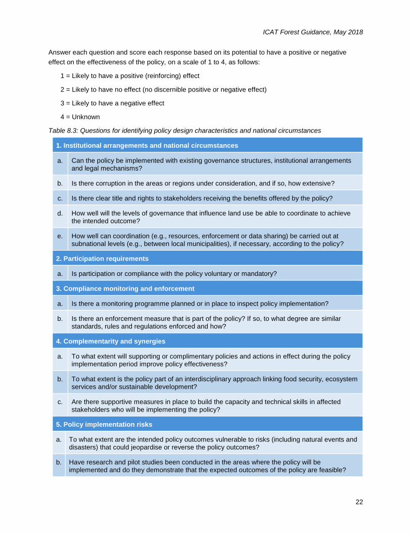
Answer each question and score each response based on its potential to have a positive or negative
effect on the effectiveness of the policy, on a scale of 1 to 4, as follows:
1 = Likely to have a positive (reinforcing) effect
2 = Likely to have no effect (no discernible positive or negative effect)
3 = Likely to have a negative effect
4 = Unknown
Table 8.3: Questions for identifying policy design characteristics and national circumstances
1. Institutional arrangements and national circumstances
a. Can the policy be implemented with existing governance structures, institutional arrangements and legal mechanisms?
b. Is there corruption in the areas or regions under consideration, and if so, how extensive?
c. Is there clear title and rights to stakeholders receiving the benefits offered by the policy?
d. How well will the levels of governance that influence land use be able to coordinate to achieve the intended outcome?
e. How well can coordination (e.g., resources, enforcement or data sharing) be carried out at subnational levels (e.g., between local municipalities), if necessary, according to the policy?
2. Participation requirements
a. Is participation or compliance with the policy voluntary or mandatory?
3. Compliance monitoring and enforcement
a. Is there a monitoring programme planned or in place to inspect policy implementation?
b. Is there an enforcement measure that is part of the policy? If so, to what degree are similar standards, rules and regulations enforced and how?
4. Complementarity and synergies
a. To what extent will supporting or complimentary policies and actions in effect during the policy implementation period improve policy effectiveness?
b. To what extent is the policy part of an interdisciplinary approach linking food security, ecosystem services and/or sustainable development?
c. Are there supportive measures in place to build the capacity and technical skills in affected stakeholders who will be implementing the policy?
5. Policy implementation risks
a. To what extent are the intended policy outcomes vulnerable to risks (including natural events and disasters) that could jeopardise or reverse the policy outcomes?
b. Have research and pilot studies been conducted in the areas where the policy will be implemented and do they demonstrate that the expected outcomes of the policy are feasible?
ICAT Forest Guidance, May 2018
23
Step 2: Evaluate the overall distribution of scores and estimate the effect on maximum implementation potential
Once policy design characteristics and national circumstances have been analysed and scored, evaluate
the overall distribution of scores:
A distribution with many scores of 1 or 2 indicates less need to refine the estimated maximum
implementation potential of the policy.
A distribution with many scores of 3 or 4 could suggest a downward adjustment of the maximum
implementation potential or gathering more information and reassessing the impact, especially for
scores of 4.
Carefully review each score of 3. Consider and, if possible, estimate to what extent the factor will
decrease policy effectiveness. Describe and justify the reduction. In addition, look for crucial problems
that have the potential to render the policy ineffective. If even one crucial problem is identified, it is
recommended to reconsider the policy design. It is recommended to identify, where possible, potential
corrective action to minimise the negative impacts. For example after following the guidance in this
section the user may reduce the geographic scope of impact, reduce the expected adoption rates or
delay the timing of the implementation of a policy.
For scores of 4, attempt to gather enough information to assess the effect of the factor. If that is not
possible, it is conservative to assume it will have a negative effect.
A positive impact may reinforce the implementation of the policy through, for example, synergetic effects
between policies. Where a situation may increase policy effectiveness, it is conservative to not estimate
any potential positive impact or make any positive adjustments to the expected policy outcomes.
8.3.2 Considerations for accounting for policy design characteristics and national circumstances
This section describes a number of considerations to bear in mind when following the steps in Section
8.3.1.
Institutional arrangements and national circumstances
Institutional arrangements are formal or informal legal and procedural agreements between agencies
executing a policy. They can include arrangements between government agencies or with government
and non-government or private sector agencies. National circumstances are the conditions present in the
country. They include, among others, the government structure, population profile, cultural context,
geographic profile, climate profile and the structure of the economy.
Lack of a governance structure, coordination between national and subnational levels or legal basis for
providing incentives to stakeholders are critical considerations that can inhibit the successful
implementation of the policy if not addressed appropriately. In countries without established institutional
arrangements or an effective legal framework to secure the cooperation between different government
levels and the involvement of key stakeholders (including private, public or non-governmental), policies
will likely be limited in their effectiveness.
Many ministries or other government agencies often have difficulties in hiring and retaining new staff
primarily due to budgetary and administrative constraints. Where staff and infrastructure (e.g., offices,
ICAT Forest Guidance, May 2018
24
equipment, vehicles or fuel) necessary for the policy implementation are not in place prior to policy
implementation, policy implementation may not move forward as expected, reducing the effectiveness of
the policy.
Corruption in national or subnational government structures can also play a detrimental role in the
implementation of the policy. Corrupt practices may involve politicians, local leaders, governmental and/or
non-governmental actors and result in implementation problems relating to land concessions, the
allocation of contracts (e.g., favouring friends or relatives), allowing illegal practices (e.g., logging without
permits), and misuse of funds intended for the policy.
Participation requirements
Participating in the policy, by people or organisations, can be voluntary or mandatory. Voluntary
participation relies on the willingness of stakeholders to respond to a policy, offers flexibility in terms of
who participates and how, and can involve less oversight and enforcement. In the absence of strong
incentives, voluntary participation is unlikely to result in high participation and is more likely to result in a
policy whose impacts are indistinguishable from the baseline scenario. Other factors that can help or
hamper participation include effective communications and training for target stakeholder groups.
Mandatory participation can be accompanied with specific obligations and can be enforced through strict
procedures, including penalties for cases of non-compliance. Mandatory participation works better in
cases where the progress of the policy implementation can be effectively monitored and enforced.
However, bribery and corruption could reduce the potential impact of the policy.
Compliance monitoring and enforcement
Monitoring and enforcement are mechanisms to compel stakeholders to comply with a policy. Monitoring
is the process of inspecting that the policy is being implemented and enforcement is an action taken
against those who are not in conformance with the policy. The policy may include measures to monitor
and/or enforce policy implementation.
When stakeholders understand that policy implementation will be monitored, it is more likely that
implementation will occur. If monitoring procedures are already in place or are planned (e.g., due to the
existence of other similar policies or projects in a region), this should be taken into account, as it can help
ensure that the policy is implemented effectively. In the absence of monitoring procedures, the policy may
not be implemented as effectively as expected.
Local enforcement agencies and other stakeholders should be consulted to determine the likelihood that
standards, rules or laws will be enforced. The likelihood of enforcement (e.g., 90% chance of
enforcement) should then be used to refine the implementation potential of the policy (e.g., reduce the
impact by 10%). If penalties for non-conformance with the policy are minor, enforcement may not be as
effective at ensuring compliance.
Complementarity and synergies
GHG mitigation policies that contribute to local sustainable development and promote better local
conditions are far more acceptable to local communities and usually have a far better chance of uptake
and success (e.g., policies that have health benefits due to reduction of local air pollution, reduce loss of
ICAT Forest Guidance, May 2018
25
biodiversity, address desertification issues, protect water resources or improve food security for poor
communities).
The implementation of GHG mitigation policies can be positively or negatively affected by other
complementary policies. For example, a policy to reduce water pollution from agricultural runoff may drive
changes in land management that reduce fertiliser use and increase use of cover crops, which are
practices that can reduce N2O emissions from soils and increase soil carbon sequestration.
Interventions that provide education and technical assistance do not reduce GHG emissions directly.
However, they may be pivotal in developing the capacity of land managers to implement new
technologies and practices that reduce GHG emissions. Therefore, the presence of such interventions
can be synergistic with GHG mitigation policies.
Policy implementation risks
Agriculture and forest productivity are greatly impacted by weather conditions, climate and water. Food,
forests and wood production are often impacted by natural events and disasters. For example, forest
fires, floods, droughts, extreme weather events (e.g., hurricanes and tornadoes), diseases and pests can
have negative consequences.
The assessment should consider the effect of natural events and disasters. If areas that are known to be
prone to extreme conditions are included in the geographic scope of the policy, the expected
implementation potential of the policy should be reduced because the policy will likely be ineffective in
those areas. However, even if there is no previous history of disaster risk, users may still consider
reducing the implementation potential of the policy to account for unanticipated disasters.
The evaluation should also consider the risk that the policy will not be as successful as anticipated at
reducing GHG emissions as a result of limited data and research. For example, where research and pilot
studies have not been conducted in the areas where the policy will be implemented there is risk that
implementation and/or impacts of the policy will be hampered by lack of experience and proof of concept,
and this could reduce policy effectiveness.
8.3.3 Example of accounting for policy design characteristics and national circumstances
The screening questions from Table 8.3 were reviewed and policy design characteristics and national
circumstances were analysed (Step 1). The participation requirements category is evaluated from the
perspective of voluntary participants in SFM and A/R, as well as from users of ecosystem services. An
additional question was added to reflect this. Extensive consultation with experts resulted in responses
and scores shown in Table 8.4.
Table 8.4: Example of accounting for policy design characteristics and national circumstances
1. Institutional arrangements and national circumstances Score
a. Can the policy be implemented with existing governance structures, institutional arrangements or legal mechanisms?
Sufficient governance structures are in place to oversee the policy implementation.
2
b. Is there corruption in the areas or regions under consideration, and if yes, how extensive? 3
ICAT Forest Guidance, May 2018
26
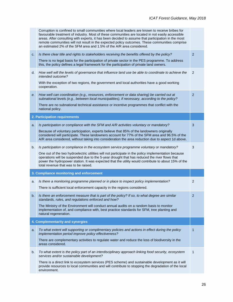
Corruption is confined to small communities where local leaders are known to receive bribes for favourable treatment of industry. Most of these communities are located in not easily accessible areas. After consulting with experts, it has been decided to assume that participation in the most remote communities will not result in the expected policy outcomes. These communities comprise an estimated 2% of the SFM area and 1.5% of the A/R area considered.
c. Is there clear title and rights to stakeholders receiving the benefits offered by the policy?
There is no legal basis for the participation of private sector in the PES programme. To address this, the policy defines a legal framework for the participation of private land owners.
2
d. How well will the levels of governance that influence land use be able to coordinate to achieve the intended outcome?
With the exception of two regions, the government and local authorities have a good working cooperation.
2
e. How well can coordination (e.g., resources, enforcement or data sharing) be carried out at subnational levels (e.g., between local municipalities), if necessary, according to the policy?
There are no subnational technical assistance or incentive programmes that conflict with the national policy.
2
2. Participation requirements
a. Is participation or compliance with the SFM and A/R activities voluntary or mandatory?
Because of voluntary participation, experts believe that 85% of the landowners originally considered will participate. These landowners account for 77% of the SFM area and 96.5% of the
A/R area considered, without taking into consideration the area reduction due to aspect 1d above.
3
b. Is participation or compliance in the ecosystem service programme voluntary or mandatory?
One out of the two hydroelectric utilities will not participate in the policy implementation because operations will be suspended due to the 5-year drought that has reduced the river flows that power the hydropower station. It was expected that the utility would contribute to about 15% of the total revenue that was to be raised.
3
3. Compliance monitoring and enforcement
a. Is there a monitoring programme planned or in place to inspect policy implementation?
There is sufficient local enforcement capacity in the regions considered.
2
b. Is there an enforcement measure that is part of the policy? If so, to what degree are similar standards, rules, and regulations enforced and how?
The Ministry of the Environment will conduct annual audits on a random basis to monitor implementation of, and compliance with, best practice standards for SFM, tree planting and natural regeneration.
2
4. Complementarity and synergies
a. To what extent will supporting or complimentary policies and actions in effect during the policy implementation period improve policy effectiveness?
There are complementary activities to regulate water and reduce the loss of biodiversity in the areas considered.
1
b. To what extent is the policy part of an interdisciplinary approach linking food security, ecosystem
services and/or sustainable development?
There is a direct link to ecosystem services (PES scheme) and sustainable development as it will provide resources to local communities and will contribute to stopping the degradation of the local environment.
1
ICAT Forest Guidance, May 2018
27
c. Are there supportive measures in place to build the capacity and technical skills in affected stakeholders who will be implementing the policy?
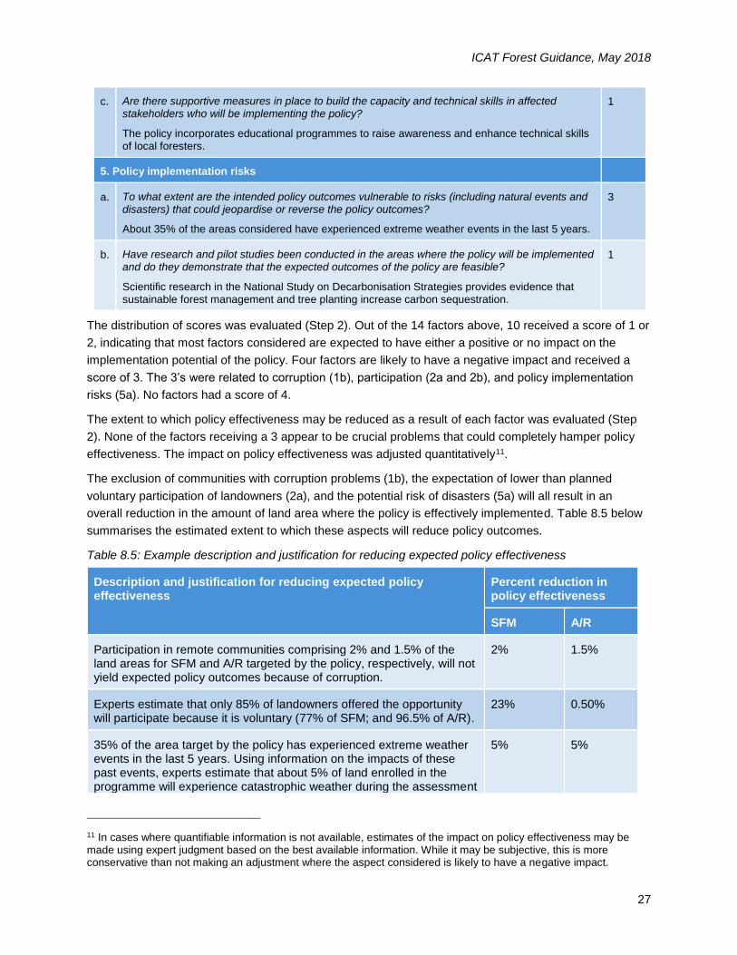
The policy incorporates educational programmes to raise awareness and enhance technical skills of local foresters.
1
5. Policy implementation risks
a. To what extent are the intended policy outcomes vulnerable to risks (including natural events and disasters) that could jeopardise or reverse the policy outcomes?
About 35% of the areas considered have experienced extreme weather events in the last 5 years.
3
b. Have research and pilot studies been conducted in the areas where the policy will be implemented and do they demonstrate that the expected outcomes of the policy are feasible?
Scientific research in the National Study on Decarbonisation Strategies provides evidence that sustainable forest management and tree planting increase carbon sequestration.
1
The distribution of scores was evaluated (Step 2). Out of the 14 factors above, 10 received a score of 1 or
2, indicating that most factors considered are expected to have either a positive or no impact on the
implementation potential of the policy. Four factors are likely to have a negative impact and received a
score of 3. The 3’s were related to corruption (1b), participation (2a and 2b), and policy implementation
risks (5a). No factors had a score of 4.
The extent to which policy effectiveness may be reduced as a result of each factor was evaluated (Step
2). None of the factors receiving a 3 appear to be crucial problems that could completely hamper policy
effectiveness. The impact on policy effectiveness was adjusted quantitatively11.
The exclusion of communities with corruption problems (1b), the expectation of lower than planned
voluntary participation of landowners (2a), and the potential risk of disasters (5a) will all result in an
overall reduction in the amount of land area where the policy is effectively implemented. Table 8.5 below
summarises the estimated extent to which these aspects will reduce policy outcomes.
Table 8.5: Example description and justification for reducing expected policy effectiveness
Description and justification for reducing expected policy effectiveness
Percent reduction in policy effectiveness
SFM A/R
Participation in remote communities comprising 2% and 1.5% of the land areas for SFM and A/R targeted by the policy, respectively, will not yield expected policy outcomes because of corruption.
2% 1.5%
Experts estimate that only 85% of landowners offered the opportunity will participate because it is voluntary (77% of SFM; and 96.5% of A/R).
23% 0.50%
35% of the area target by the policy has experienced extreme weather events in the last 5 years. Using information on the impacts of these past events, experts estimate that about 5% of land enrolled in the programme will experience catastrophic weather during the assessment
5% 5%
11 In cases where quantifiable information is not available, estimates of the impact on policy effectiveness may be made using expert judgment based on the best available information. While it may be subjective, this is more conservative than not making an adjustment where the aspect considered is likely to have a negative impact.
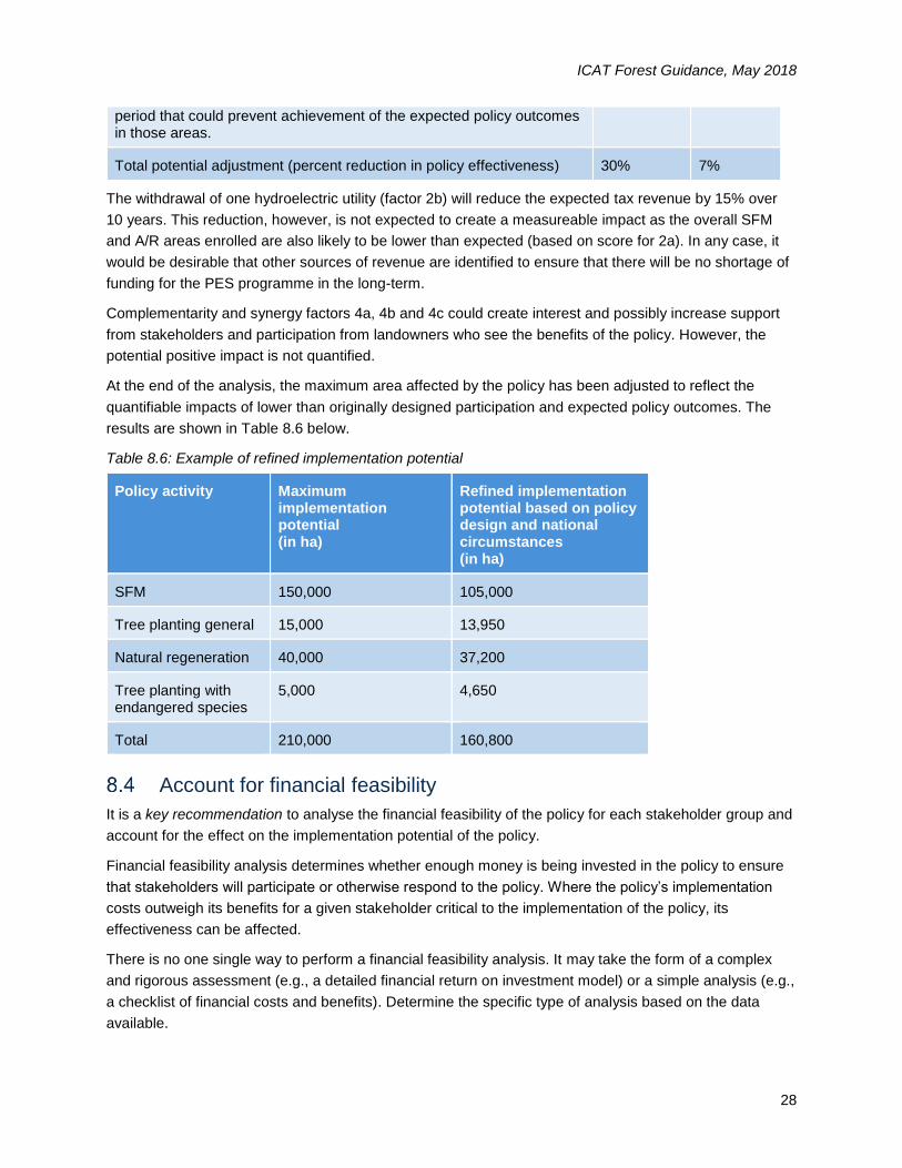
ICAT Forest Guidance, May 2018
28
period that could prevent achievement of the expected policy outcomes in those areas.
Total potential adjustment (percent reduction in policy effectiveness) 30% 7%
The withdrawal of one hydroelectric utility (factor 2b) will reduce the expected tax revenue by 15% over
10 years. This reduction, however, is not expected to create a measureable impact as the overall SFM
and A/R areas enrolled are also likely to be lower than expected (based on score for 2a). In any case, it
would be desirable that other sources of revenue are identified to ensure that there will be no shortage of
funding for the PES programme in the long-term.
Complementarity and synergy factors 4a, 4b and 4c could create interest and possibly increase support
from stakeholders and participation from landowners who see the benefits of the policy. However, the
potential positive impact is not quantified.
At the end of the analysis, the maximum area affected by the policy has been adjusted to reflect the
quantifiable impacts of lower than originally designed participation and expected policy outcomes. The
results are shown in Table 8.6 below.
Table 8.6: Example of refined implementation potential
Policy activity Maximum implementation potential (in ha)
Refined implementation potential based on policy design and national circumstances (in ha)
SFM 150,000 105,000
Tree planting general 15,000 13,950
Natural regeneration 40,000 37,200
Tree planting with endangered species
5,000 4,650
Total 210,000 160,800
Account for financial feasibility
It is a key recommendation to analyse the financial feasibility of the policy for each stakeholder group and
account for the effect on the implementation potential of the policy.
Financial feasibility analysis determines whether enough money is being invested in the policy to ensure
that stakeholders will participate or otherwise respond to the policy. Where the policy’s implementation
costs outweigh its benefits for a given stakeholder critical to the implementation of the policy, its
effectiveness can be affected.
There is no one single way to perform a financial feasibility analysis. It may take the form of a complex
and rigorous assessment (e.g., a detailed financial return on investment model) or a simple analysis (e.g.,
a checklist of financial costs and benefits). Determine the specific type of analysis based on the data
available.
ICAT Forest Guidance, May 2018
29
Sources of information for conducting financial feasibility are, in order of preference:
Existing calculations of the costs and benefits of policies for an individual stakeholder that were
done during the policy design phase (as long as these are deemed reliable)
Implementation cost analyses
Exiting national cost studies
Global cost studies
Expert judgment based on assessments or desk review
In the absence of other available resources, guidance is provided in the sections below for performing a
basic cost analysis. Section 8.4.1 provides a method for analysing financial feasibility. Section 8.4.2
provides some further guidance to help with this analysis. Section 8.4.3 provides a worked example to
illustrate the steps.
Before starting the cost analysis, some questions to consider are:
Do some stakeholders bear significant new net costs under the proposed policy? If so, which
ones and what are the costs?
Do some stakeholders realise significant new net financial gain under the proposed policy? If so,
which ones and what are the gains?
What goods and services are produced commercially from lands that are the target of the policy,
both before and after policy implementation? Is production likely to increase or decrease as a
result of the policy?
Is the policy potentially in conflict with economic development?
Will the policy strengthen important supply chains?
8.4.1 Method for accounting for financial feasibility
Step 1: Identify stakeholder groups to analyse
In Section 6.1.1, users identified the stakeholders of the policy. Those stakeholders are the focus of this
analysis, in particular stakeholders that implement changes in practices, technologies or land use in
response to the policy. Each stakeholder group should be included in the financial feasibility analysis and
the net costs and benefits for each group considered separately. Where there is not sufficient data and
information to analyse all stakeholder groups separately, at minimum include the following groups in the
analysis:
Stakeholders with official land tenure rights or de facto control of lands addressed by the policy
Stakeholders that use the lands addressed by the policy but have limited actual control over the
lands
It can be difficult to distinguish between stakeholders with official tenure to land and stakeholders that use
the lands affected by the policy without tenure. In such cases, focus on the main stakeholder group that
expected to implement the mitigation measures.
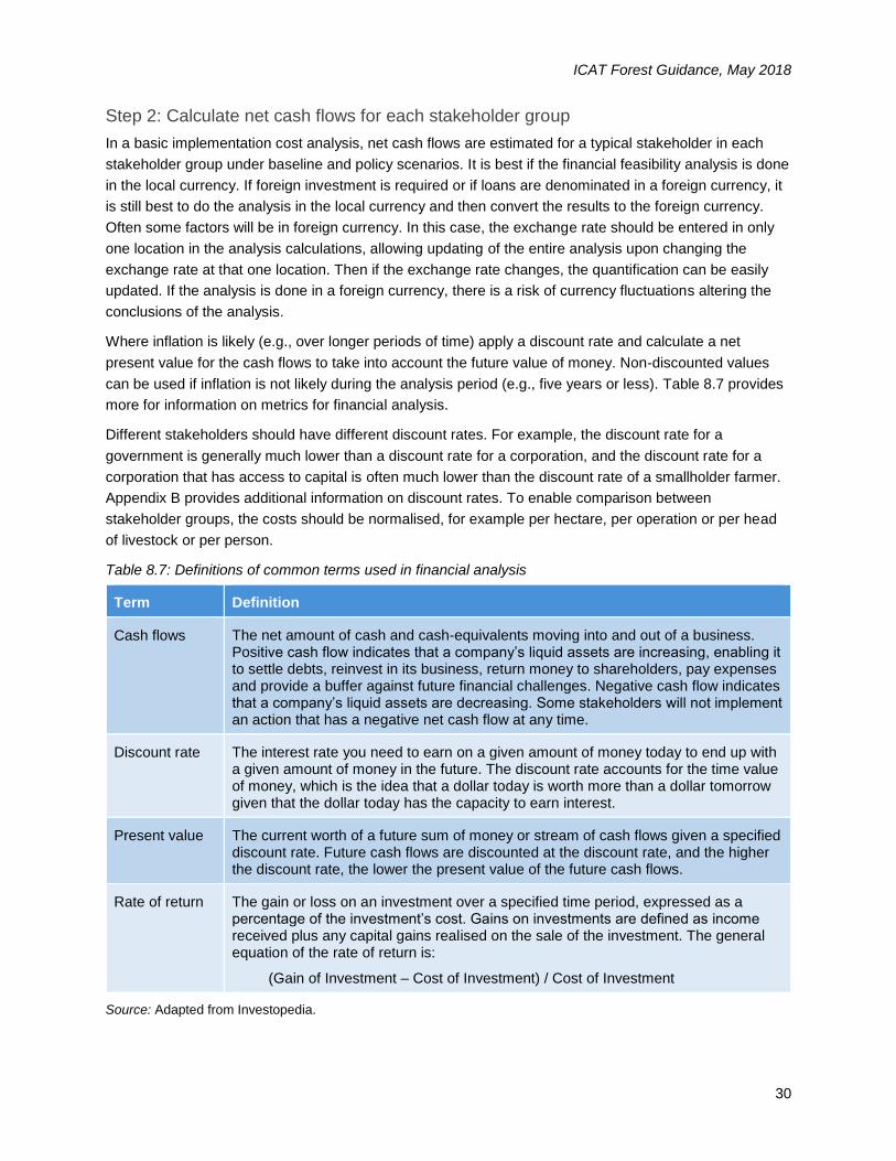
ICAT Forest Guidance, May 2018
30
Step 2: Calculate net cash flows for each stakeholder group
In a basic implementation cost analysis, net cash flows are estimated for a typical stakeholder in each
stakeholder group under baseline and policy scenarios. It is best if the financial feasibility analysis is done
in the local currency. If foreign investment is required or if loans are denominated in a foreign currency, it
is still best to do the analysis in the local currency and then convert the results to the foreign currency.
Often some factors will be in foreign currency. In this case, the exchange rate should be entered in only
one location in the analysis calculations, allowing updating of the entire analysis upon changing the
exchange rate at that one location. Then if the exchange rate changes, the quantification can be easily
updated. If the analysis is done in a foreign currency, there is a risk of currency fluctuations altering the
conclusions of the analysis.
Where inflation is likely (e.g., over longer periods of time) apply a discount rate and calculate a net
present value for the cash flows to take into account the future value of money. Non-discounted values
can be used if inflation is not likely during the analysis period (e.g., five years or less). Table 8.7 provides
more for information on metrics for financial analysis.
Different stakeholders should have different discount rates. For example, the discount rate for a
government is generally much lower than a discount rate for a corporation, and the discount rate for a
corporation that has access to capital is often much lower than the discount rate of a smallholder farmer.
Appendix B provides additional information on discount rates. To enable comparison between
stakeholder groups, the costs should be normalised, for example per hectare, per operation or per head
of livestock or per person.
Table 8.7: Definitions of common terms used in financial analysis
Term Definition
Cash flows The net amount of cash and cash-equivalents moving into and out of a business. Positive cash flow indicates that a company’s liquid assets are increasing, enabling it to settle debts, reinvest in its business, return money to shareholders, pay expenses and provide a buffer against future financial challenges. Negative cash flow indicates that a company’s liquid assets are decreasing. Some stakeholders will not implement an action that has a negative net cash flow at any time.
Discount rate The interest rate you need to earn on a given amount of money today to end up with a given amount of money in the future. The discount rate accounts for the time value of money, which is the idea that a dollar today is worth more than a dollar tomorrow given that the dollar today has the capacity to earn interest.
Present value The current worth of a future sum of money or stream of cash flows given a specified discount rate. Future cash flows are discounted at the discount rate, and the higher the discount rate, the lower the present value of the future cash flows.
Rate of return The gain or loss on an investment over a specified time period, expressed as a percentage of the investment’s cost. Gains on investments are defined as income received plus any capital gains realised on the sale of the investment. The general equation of the rate of return is:
(Gain of Investment – Cost of Investment) / Cost of Investment
Source: Adapted from Investopedia.
ICAT Forest Guidance, May 2018
31
To estimate net cash flows:
1. Estimate baseline scenario costs and revenues using present day data for a typical stakeholder
that will take part in the policy, repeating this separately for each stakeholder group. Taking into
account how the land area under consideration would be used without the policy (e.g., what is
produced on the land and how much, considering for example, animal farming, croplands, set
asides or logging)
Average cost and revenue figures can be used for groups of land categories. For example, use
average expense and income from all cropland areas (irrespective of the type of the crop); group
together fallow land and set asides and derive average values for those lands; or use national
average timber harvest statistics and prices.
Include costs of inputs and costs of production, in addition to revenues from sale of goods. Key
input costs include raw materials, equipment, labour, permits to operate, and other costs entailed
in producing and selling the goods. For example, in agriculture costs include fertiliser and seed
for crops, cost of fencing for cattle, feed, feed additives and medications. Input costs may include
taxes on operations or land that must be paid from revenues from the sale of goods.12
2. Estimate the baseline scenario net cash flow (i.e., revenues minus costs) over the assessment
period, separately for each stakeholder group.
3. Estimate the policy scenario costs and revenues over the assessment period, separately for each
stakeholder group. This includes determining:
The amount and type of government or private funding committed to implementing the
policy
The cost to the stakeholder to implement the policy
The revenues that the stakeholder will gain from the policy
4. Estimate the net cash flow for a typical stakeholder in the policy scenario, separately for each
stakeholder group
Step 3: Assess financial feasibility
Compare the net cash flow for the baseline scenario with that for the policy scenario to assess financial
feasibility, as follows:
1. Determine whether the total net cash flow for the policy scenario exceeds the net cash flow for
the baseline scenario. This must be the case for the policy to be financially feasible.
2. Determine whether the total net cash flow for the policy scenario is positive. This must be the
case for the policy to be financially feasible.
3. When the net cash flow for the policy scenario is positive, compare the discounted cash flow (net
present value) and rate of return (for the general formula see Table 8.7) in the baseline and policy
12 The European Commission Guide to Cost-Benefit Analysis of Investment Projects can be a useful resource for how to identify costs and revenues, calculate discounted cash flows, and implement other aspects of financial and economic feasibility analysis. Available at: http://ec.europa.eu/regional_policy/sources/docgener/guides/cost/guide2008_en.pdf
ICAT Forest Guidance, May 2018
32
cases. For the policy to be financially feasible, the rate of return on the policy case must be higher
than the baseline rate of return by more than three percentage points.
Repeat this analysis for each stakeholder group identified and all activities covered by the policy.
Step 4: Estimate the extent to which financial aspects will limit policy outcomes
Based on the results of the financial feasibility assessment, decide how the implementation potential of
the policy will be affected, as follows:
Where the policy does not appear to provide sufficient incentive for stakeholders to participate or
otherwise respond to the policy, either reconsider the design of the policy (or the relevant
component of the policy) or refine the implementation potential of the policy.
Where the policy appears to provide sufficient incentive for stakeholders to participation or
otherwise respond to the policy, continue to the next step without revising the implementation
potential of the policy.
8.4.2 Considerations for accounting for financial feasibility
Below are additional considerations when deciding how the implementation potential of the policy will be
affected.
In addition to discounted costs and revenues, the financial analysis should consider the relative
timing of costs and revenues, and the capital needed to achieve these cash flows. If costs occur
before revenues, stakeholders must have access to funds to pay the costs or they may not
behave as expected.
Shifts in timing of returns can be large for afforestation and reforestation. There are considerable
costs in establishing stands of trees, but there may be negligible revenues for years while the
trees grow to have commercial value. As a result, many forestry projects are only financially
feasible with low discount rates. For entities with high discount rates, such as most smallholder
farmers, even modest seasonal delays in revenue relative to expenditures can create a significant
barrier to implementation. Delaying the harvest season can be a barrier to food insecure
households that do not have other crops to eat during the delay.
In general, unless the policy increases net revenue to stakeholders, or reduces their risks, the
policy is unlikely to be adopted voluntarily.
Policies that provide a net financial benefit may have little incentive for adoption if the net gain is
small relative to overall cash flows.
Investors, farmers, landowners and other stakeholders are often risk averse. Some policies offer
stakeholders a positive financial return, yet still fail to be adopted, because stakeholder’s view
returns as too uncertain or risky. For example, they may not be confident payments in the future
will be made, contracts will be honoured, or the policy will have ongoing political and budgetary
support. As a result, assessing simple return on investment alone may not give a reliable
indication of the likelihood of policy adoption. Financial risk can be quantitatively incorporated into
the analysis by increasing stakeholder’s discount rate, or qualitatively considered by consulting
stakeholders on their likely response to specific real-world policy incentives.
ICAT Forest Guidance, May 2018
33
Some changes may have non-obvious costs. For example, a change may involve significant
management labour costs to revise organisational processes or training new workers that are
needed to provide different skills into the organisation.
It may be important to identify other financial considerations and sectoral policies and trends that
may affect the outcome of the financial feasibility of the policy, and to consider whether these
sectoral policies or trends reinforce or counteract the intended implementation (e.g., through price
signals and consumer behaviour).
When a government is considering what policies to adopt, it may also want to consider the financial
effects on society as a whole. However, such an evaluation is beyond the scope of this guidance.13
8.4.3 Example of accounting for financial feasibility
To estimate net cash flows, data on a per-hectare basis are used for annual costs and benefits for land
areas affected by the policy, from the perspective of stakeholders managing the land. For this example, a
cost analysis is conducted for tree planting activities on cropland. This example considers the first 10
years of implementation after the conversion of agricultural land into forest land, representing enough
time to complete a harvest cycle and realise the value of timber from the planted trees.
The costs and revenues for the baseline scenario are estimated in Table 8.8. The baseline scenario
assumes that there will be a continuation of current agricultural production for the next 10 years (constant
baseline). The tables present annual data for Year 1, Years 2-9 and Year 10 of the policy. Negative
numbers represent costs (expenses) and positive numbers represent revenues (income).
Table 8.8: Example calculation of baseline costs and revenues for continuation of agricultural production
Baseline
Annual costs and revenues for Year (USD/ha):
Total
1 2-9* 10
Costs
Farming labour -100 -100 -100
Crop inputs (seed, fertiliser, equipment, fuel) -100 -100 -100
Land cost, taxes and concession fees 0 0 0
Total cost -200 -200 -200
Revenues
Crop revenues 250 250 250
Net farming revenue, undiscounted 50 50 50 500
Net farming revenue, present value 50 [43 – 16] 14 289
* Years 2-9 are not shown for simplicity. Square brackets indicate the range of values during that time period. For
example, [43 -16] means values range from USD 43/ha in Year 2 to USD 16/ha in Year 9
13 A variety of sources are available that provide guidance on estimating net economic effects on society, including EC 2008.
ICAT Forest Guidance, May 2018
34
Table 8.8 provides average present day estimates for costs and revenues per hectare under the baseline
scenario. The costs identified were farming labour, crop inputs (seed, fertiliser, equipment, fuel), and land
cost, taxes and concession fees. The revenues identified include all income from selling the crops. The
cost and revenue were kept constant for all 10 years. Based on these assumptions, a typical farmer has
net annual revenues (or cash flow) of USD 50 per hectare. Applying a discount rate of 15% reduces the
annual revenue from USD 50/ha in Year 1 to USD 14/ha by Year 10.
Next the costs and revenues for the policy scenario are estimated (Table 8.9). Under the policy scenario,
the same cropland area is converted to forest land through general tree planting.
Table 8.9: Example calculation of policy scenario costs and revenues for general tree planting
Policy Scenario: Tree planting general
Annual costs and revenues for Year (USD/ha):
Total
1 2-9* 10
Costs
Planting cost -1,000 0 0
Land costs, taxes and concession fees 0 0 0
Stand management and harvest cost 0 -10 -12,500
Total cost -1,000 -10 -12,500
Revenues
Timber 0 0 15,000
Government payments for planting 1,000 0 0
Government livelihood support 0 0 0
Total revenue 1,000 0 15,000
Net tree planting revenue, $/ha, undiscounted 0 -10 2,500 2,420
Net tree planting revenue, $/ha, present value 0 [-9 – -3] 711 665
* Years 2-9 are not shown for simplicity. Square brackets indicate the range of values during that time period.
Table 8.9 provides average present day estimates for costs and revenues per hectare under the policy
scenario. The costs identified are planting cost for trees, land costs, taxes and concession fees, and
stand management and harvest cost. It is anticipated that the farmer would have planting costs for Year 1
(USD 1,000/ha), stand management costs for Years 2-9 (USD 10/ha), and harvest costs for Year 10
(USD 12,000/ha, assuming a harvest of 50 m3/ha, a harvest cost of USD 100/m3, a processing cost of
USD 50/m3, and transport and tax cost of USD 100/m3)
The revenues identified include government support for the planting of all trees in Year 1 (USD 1,000/ha),
and income from selling the harvested timber in Year 10 (assuming a harvest of 50 m3/ha, and a price of
USD 300/m3).
Comparison of discounted net revenues between the baseline (USD 289/ha) and policy (USD 665/ha)
scenarios indicates that general tree planting activities may be profitable for farmers (Table 8.8 and Table
8.9). The net cash flow in the policy scenario is positive and exceeds the net cash flow for the baseline
scenario. In both cases, the net revenue after 10 years of tree planting would be significantly higher than
the net farming revenue.
ICAT Forest Guidance, May 2018
35
However, yearly cash flow trends in the policy scenario show a net loss of income for 9 out of the 10
years of policy implementation. Because of this, some farmers may decide not to participate. Other
farmers may be able to wait until Year 10 for the revenue from selling the harvested timber and would be
more likely to participate. Without more information or refining of the policy design, participation is likely to
be highly situational and difficult to predict.
Given this uncertainty, the policy design is reconsidered and an alternative scenario explored. The
alternative scenario would be for the government to provide a low-interest rate (e.g., 4%) annual loan
payment to compensate for the lost revenue (USD 50/ha/year) (see Table 8.10). The loan provides the
farmer with annual income (although less than the baseline case) and the total loan value can be repaid
from timber sale revenues in Year 10. If the policy is modified this way, broad participation in the
programme is more likely. Table 8.10 demonstrates the costs and revenues of the redesigned policy for
general tree planting with a low-interest rate loan.
Table 8.10: Calculation of policy scenario costs and revenues for general tree planting with a low-interest rate loan
Policy Scenario: Tree planting general
Annual costs and revenues for Year (USD/ha): Total
1 2-9* 10
Costs
Planting cost -1,000 0 0
Land costs, taxes, concession fees 0 0 0
Stand management & harvest cost 0 -10 -12,500
Total cost -1,000 -10 -12,500
Revenues (with government support)
Timber 0 0 15,000
Government payments for planting 1,000 0 0
Government livelihood support 50 50 -1,300
Total revenue 1,050 50 13,700
Net tree planting revenue, undiscounted 50 40 1,200 1,570
Net tree planting revenue, present value 50 [35 – 13] 341 571
* Years 2-9 are not shown for simplicity. Square brackets indicate the range of values during that time period.
Net cash flow estimates were made for natural regeneration and tree planting with endangered species
for the A/R policy scenario (not shown), using the same constant baseline scenario as in Table 8.8
(continuation of current agricultural production for the next 10 years). Net cash flow estimate were also
made for implementing SFM on privately owned forest land, where the constant baseline is the
continuation of current forest management practices (not shown).
After considering all proposed activities, and adjusting some policy design aspects as described above,
the policy was determined to be financially feasible for general tree planting and tree planting with
endangered species. For SFM and natural regeneration, the policy scenario does not generate more
revenue for landowners. Therefore the policy design was modified further to increase payments for SFM
and natural regeneration maintaining the overall budget level. To achieve this, the area of land targeted
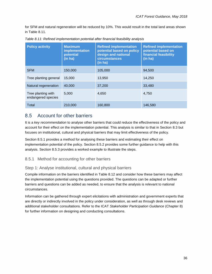
ICAT Forest Guidance, May 2018
36
for SFM and natural regeneration will be reduced by 10%. This would result in the total land areas shown
in Table 8.11.
Table 8.11: Refined implementation potential after financial feasibility analysis
Policy activity Maximum implementation potential (in ha)
Refined implementation potential based on policy design and national circumstances (in ha)
Refined implementation potential based on financial feasibility (in ha)
SFM 150,000 105,000 94,500
Tree planting general 15,000 13,950 14,250
Natural regeneration 40,000 37,200 33,480
Tree planting with endangered species
5,000 4,650 4,750
Total 210,000 160,800 146,580
Account for other barriers
It is a key recommendation to analyse other barriers that could reduce the effectiveness of the policy and
account for their effect on the implementation potential. This analysis is similar to that in Section 8.3 but
focuses on institutional, cultural and physical barriers that may limit effectiveness of the policy.
Section 8.5.1 provides a method for analysing these barriers and estimating their effect on
implementation potential of the policy. Section 8.5.2 provides some further guidance to help with this
analysis. Section 8.5.3 provides a worked example to illustrate the steps.
8.5.1 Method for accounting for other barriers
Step 1: Analyse institutional, cultural and physical barriers
Compile information on the barriers identified in Table 8.12 and consider how these barriers may affect
the implementation potential using the questions provided. The questions can be adapted or further
barriers and questions can be added as needed, to ensure that the analysis is relevant to national
circumstances.
Information can be gathered through expert elicitations with administration and government experts that
are directly or indirectly involved in the policy under consideration, as well as through desk reviews and
additional stakeholder consultations. Refer to the ICAT Stakeholder Participation Guidance (Chapter 8)
for further information on designing and conducting consultations.
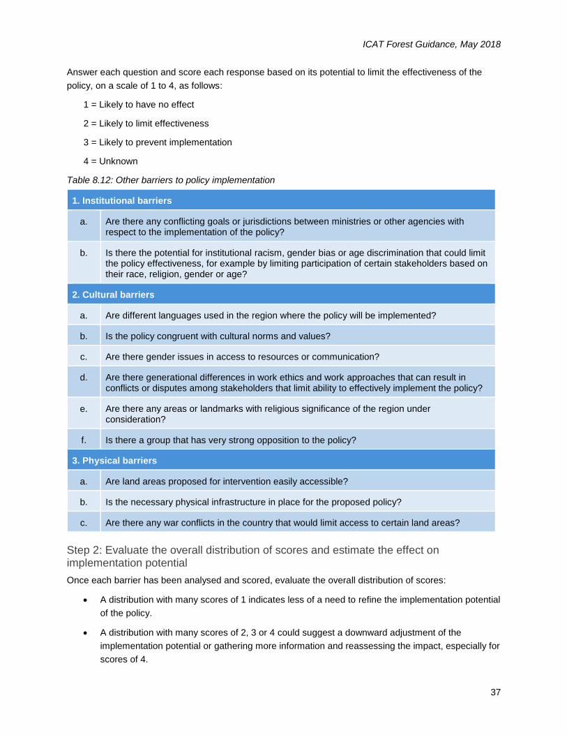
ICAT Forest Guidance, May 2018
37
Answer each question and score each response based on its potential to limit the effectiveness of the
policy, on a scale of 1 to 4, as follows:
1 = Likely to have no effect
2 = Likely to limit effectiveness
3 = Likely to prevent implementation
4 = Unknown
Table 8.12: Other barriers to policy implementation
1. Institutional barriers
a. Are there any conflicting goals or jurisdictions between ministries or other agencies with respect to the implementation of the policy?
b. Is there the potential for institutional racism, gender bias or age discrimination that could limit the policy effectiveness, for example by limiting participation of certain stakeholders based on their race, religion, gender or age?
2. Cultural barriers
a. Are different languages used in the region where the policy will be implemented?
b. Is the policy congruent with cultural norms and values?
c. Are there gender issues in access to resources or communication?
d. Are there generational differences in work ethics and work approaches that can result in conflicts or disputes among stakeholders that limit ability to effectively implement the policy?
e. Are there any areas or landmarks with religious significance of the region under consideration?
f. Is there a group that has very strong opposition to the policy?
3. Physical barriers
a. Are land areas proposed for intervention easily accessible?
b. Is the necessary physical infrastructure in place for the proposed policy?
c. Are there any war conflicts in the country that would limit access to certain land areas?
Step 2: Evaluate the overall distribution of scores and estimate the effect on implementation potential
Once each barrier has been analysed and scored, evaluate the overall distribution of scores:
A distribution with many scores of 1 indicates less of a need to refine the implementation potential
of the policy.
A distribution with many scores of 2, 3 or 4 could suggest a downward adjustment of the
implementation potential or gathering more information and reassessing the impact, especially for
scores of 4.
ICAT Forest Guidance, May 2018
38
Carefully review each score of 2 and 3. For a score of 2 consider and, if possible, estimate to what extent
the barrier will decrease policy effectiveness. Describe and justify the reduction. For a score of 3, the
barrier is considered crucial and has the potential to render the policy ineffective. If even one crucial
barrier is identified, it is recommended to reconsider the policy design and discontinue the impacts
assessment. For scores of 4, attempt to gather enough information to assess the effect of the barrier. If
that is not possible, it is conservative to assume it limits effectiveness.
Consider and determine to what extent the effects of the barriers overlap. An overlapping effect occurs
where one barrier limits implementation in one area and another barrier also limits implementation in the
same area. These overlapping effects should be appropriately accounted for when calculating the
potential effect of all barriers. The combined effect of the barriers together may be greater than or less
than the sum of the individual barriers. If information is available, uncertainty ranges should also be
incorporated in the final results.
During the data-gathering phase, it is recommended that information also be collected on any other
relevant policies in the country that might help overcome specific barriers. Where such policies exist, the
scoring of the barrier effect should be changed accordingly (most likely to a score of 1).
8.5.2 Considerations for accounting for other barriers
Institutional barriers
Conflicting goals between different ministries and other government agencies could result in overlapping
regulation and ambiguous roles and responsibilities of the stakeholders involved. For example, proposed
areas for the policy may overlap with other existing types of area protection (e.g., based on national
policies or international conventions), which could lead to confusing regulations for specific sites.
Institutional barriers relating to discrimination often include racism, gender bias, age discrimination,
favouritism and other selection approaches that are not based on the actual performance of individual
workers. Where discrimination is present, certain stakeholders may not have equal access to the
opportunities afforded by a policy (e.g., incentive payments, technical assistance or education) and this
can limit overall effectiveness. Often such barriers are linked to corrupt practices (addressed in Section
8.3). Safeguards to prevent discrimination can be built into policies. For example, it can be required that
enrolment in programmes such as education opportunities must be diverse in terms of race and gender. If
safeguards against discrimination do not exist, either as part of the policy being analysed or in institutions
involved in implementing the policy, it is possible that discrimination will be a barrier to policy
implementation.
Cultural barriers
The use of language and terminology that is not widely understood by the target stakeholders could be a
crucial cultural barrier as it could result in communications problems causing misunderstandings, mistrust
and non-participation/compliance among the local population. Where language barriers exist and there is
no mechanism in place to overcome them, the effectiveness of the policy is likely to be reduced.
In many countries, the successful implementation of mitigation policies may require consideration of
gender or social class sensitivities to reduce resistance of local communities to the proposed intervention.
Cultural preferences may have more potential for change than physical limits, but change may take time
and almost certainly will benefit from considering existing mechanisms of social influence. There may also
ICAT Forest Guidance, May 2018
39
be generational differences in work ethics and work approaches that have the potential to result in
conflicts between older and younger workers. If the policy is sensitive to such factors, including potential
language barriers, age distribution and cultural norms of stakeholders, they may not present a barrier to
implementation.
In some countries, gender considerations can have a very important effect on the success or failure of
implementation of the policy. It is important to consider who makes decisions about land use actions, and
who has access to information and money. For a policy to be implemented effectively the person who is
responsible for managing land will also need to have the ability to access information and financing to
implement management changes. If they do not, this will likely limit policy effectiveness.
Certain land areas or landmarks have important religious significance for local communities. Policies that
may affect ancestral homes or sacred grounds would be more likely to face resistance from indigenous
peoples and local communities.
Strong opposition to a policy, for example from a particular stakeholder group or political party, could
hamper efforts to secure financing, gain trust, and otherwise implement policy interventions, especially if
that group is influential.
Failure to identify and address cultural barriers will more than likely have detrimental impacts on the policy
implementation. Effective stakeholder participation from early in policy design is important to identify and
address cultural barriers. Refer to the ICAT Stakeholder Participation Guidance for further information
about all elements of effective stakeholder participation for policy design, implementation and evaluation.
Physical barriers
In mountainous countries or countries with inaccessible regions, policies relating to agriculture and forests
should take into account whether certain land areas are remote or are difficult to access. Minimal existing
road networks or insufficient transportation infrastructure would be expected to limit the implementation
potential.
Conflicts in a country (such as civil war or territorial disputes with a neighbouring country) could limit
access to areas that could be considered for policy intervention. Depending on the severity of the conflict,
and to safeguard the welfare of the people involved, certain parts of the country may be excluded until the
conflict is resolved. This would reduce the impact of the policy at least through the time period during
which conflicts remain active, and possibly longer.
8.5.3 Example of accounting for other barriers
The screening questions from Table 8.12 were reviewed (Step 1). Not all of the screening questions were
identified to be relevant and a few of the questions were modified to suit national circumstances. The
barriers under the cultural barriers category related to cultural norms and values (2b), gender issues (2c),
generational differences (2d), and areas of religious significance (2e) were considered collectively. The
barriers under the physical barrier category related accessibility of land area (3a) and availability of
infrastructure (3b) were also considered jointly. With these modifications a total of seven barriers were
considered. In consultation with experts, responses were tabulated and scored in Table 8.13 below.
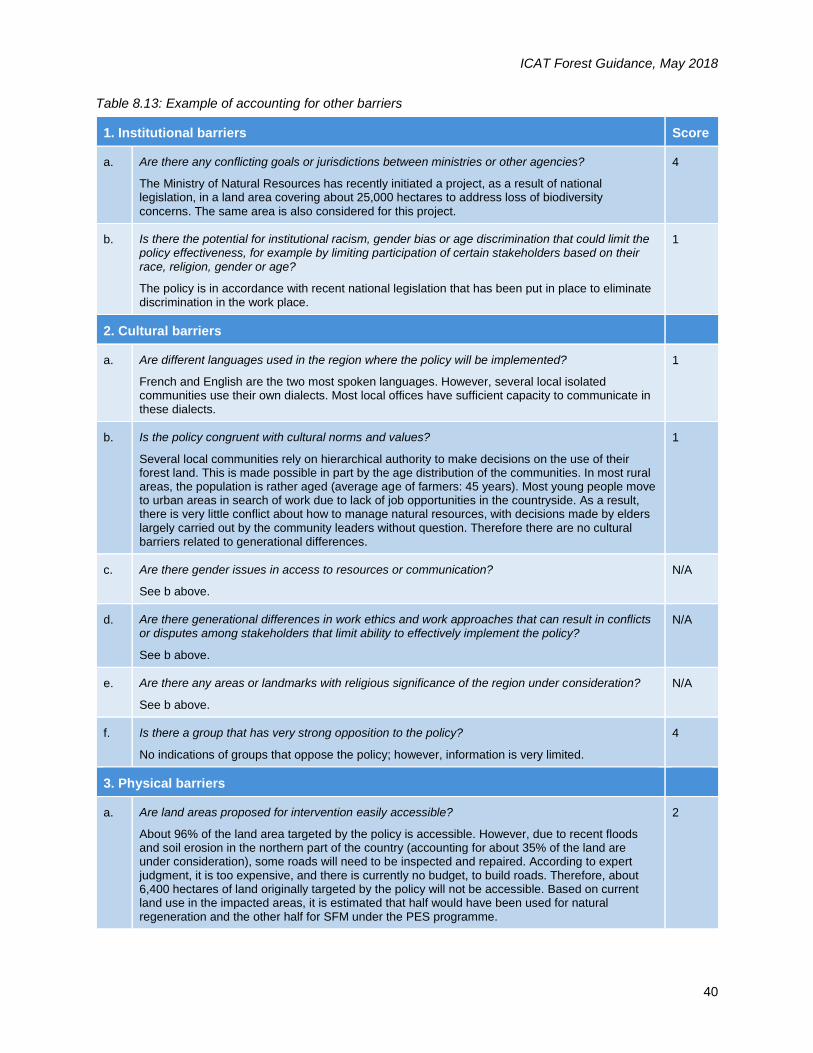
ICAT Forest Guidance, May 2018
40
Table 8.13: Example of accounting for other barriers
1. Institutional barriers Score
a. Are there any conflicting goals or jurisdictions between ministries or other agencies?
The Ministry of Natural Resources has recently initiated a project, as a result of national legislation, in a land area covering about 25,000 hectares to address loss of biodiversity
concerns. The same area is also considered for this project.
4
b. Is there the potential for institutional racism, gender bias or age discrimination that could limit the policy effectiveness, for example by limiting participation of certain stakeholders based on their race, religion, gender or age?
The policy is in accordance with recent national legislation that has been put in place to eliminate discrimination in the work place.
1
2. Cultural barriers
a. Are different languages used in the region where the policy will be implemented?
French and English are the two most spoken languages. However, several local isolated communities use their own dialects. Most local offices have sufficient capacity to communicate in these dialects.
1
b. Is the policy congruent with cultural norms and values?
Several local communities rely on hierarchical authority to make decisions on the use of their forest land. This is made possible in part by the age distribution of the communities. In most rural areas, the population is rather aged (average age of farmers: 45 years). Most young people move to urban areas in search of work due to lack of job opportunities in the countryside. As a result, there is very little conflict about how to manage natural resources, with decisions made by elders largely carried out by the community leaders without question. Therefore there are no cultural barriers related to generational differences.
1
c. Are there gender issues in access to resources or communication?
See b above.
N/A
d. Are there generational differences in work ethics and work approaches that can result in conflicts or disputes among stakeholders that limit ability to effectively implement the policy?
See b above.
N/A
e. Are there any areas or landmarks with religious significance of the region under consideration?
See b above.
N/A
f. Is there a group that has very strong opposition to the policy?
No indications of groups that oppose the policy; however, information is very limited.
4
3. Physical barriers
a. Are land areas proposed for intervention easily accessible?
About 96% of the land area targeted by the policy is accessible. However, due to recent floods and soil erosion in the northern part of the country (accounting for about 35% of the land are under consideration), some roads will need to be inspected and repaired. According to expert judgment, it is too expensive, and there is currently no budget, to build roads. Therefore, about 6,400 hectares of land originally targeted by the policy will not be accessible. Based on current land use in the impacted areas, it is estimated that half would have been used for natural regeneration and the other half for SFM under the PES programme.
2
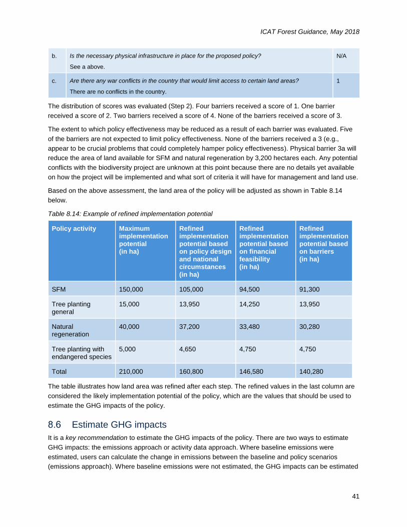
ICAT Forest Guidance, May 2018
41
b. Is the necessary physical infrastructure in place for the proposed policy?
See a above.
N/A
c. Are there any war conflicts in the country that would limit access to certain land areas?
There are no conflicts in the country.
1
The distribution of scores was evaluated (Step 2). Four barriers received a score of 1. One barrier
received a score of 2. Two barriers received a score of 4. None of the barriers received a score of 3.
The extent to which policy effectiveness may be reduced as a result of each barrier was evaluated. Five
of the barriers are not expected to limit policy effectiveness. None of the barriers received a 3 (e.g.,
appear to be crucial problems that could completely hamper policy effectiveness). Physical barrier 3a will
reduce the area of land available for SFM and natural regeneration by 3,200 hectares each. Any potential
conflicts with the biodiversity project are unknown at this point because there are no details yet available
on how the project will be implemented and what sort of criteria it will have for management and land use.
Based on the above assessment, the land area of the policy will be adjusted as shown in Table 8.14
below.
Table 8.14: Example of refined implementation potential
Policy activity Maximum implementation potential (in ha)
Refined implementation potential based on policy design and national circumstances (in ha)
Refined implementation potential based on financial feasibility (in ha)
Refined implementation potential based on barriers (in ha)
SFM 150,000 105,000 94,500 91,300
Tree planting general
15,000 13,950 14,250 13,950
Natural regeneration
40,000 37,200 33,480 30,280
Tree planting with endangered species
5,000 4,650 4,750 4,750
Total 210,000 160,800 146,580 140,280
The table illustrates how land area was refined after each step. The refined values in the last column are
considered the likely implementation potential of the policy, which are the values that should be used to
estimate the GHG impacts of the policy.
Estimate GHG impacts
It is a key recommendation to estimate the GHG impacts of the policy. There are two ways to estimate
GHG impacts: the emissions approach or activity data approach. Where baseline emissions were
estimated, users can calculate the change in emissions between the baseline and policy scenarios
(emissions approach). Where baseline emissions were not estimated, the GHG impacts can be estimated
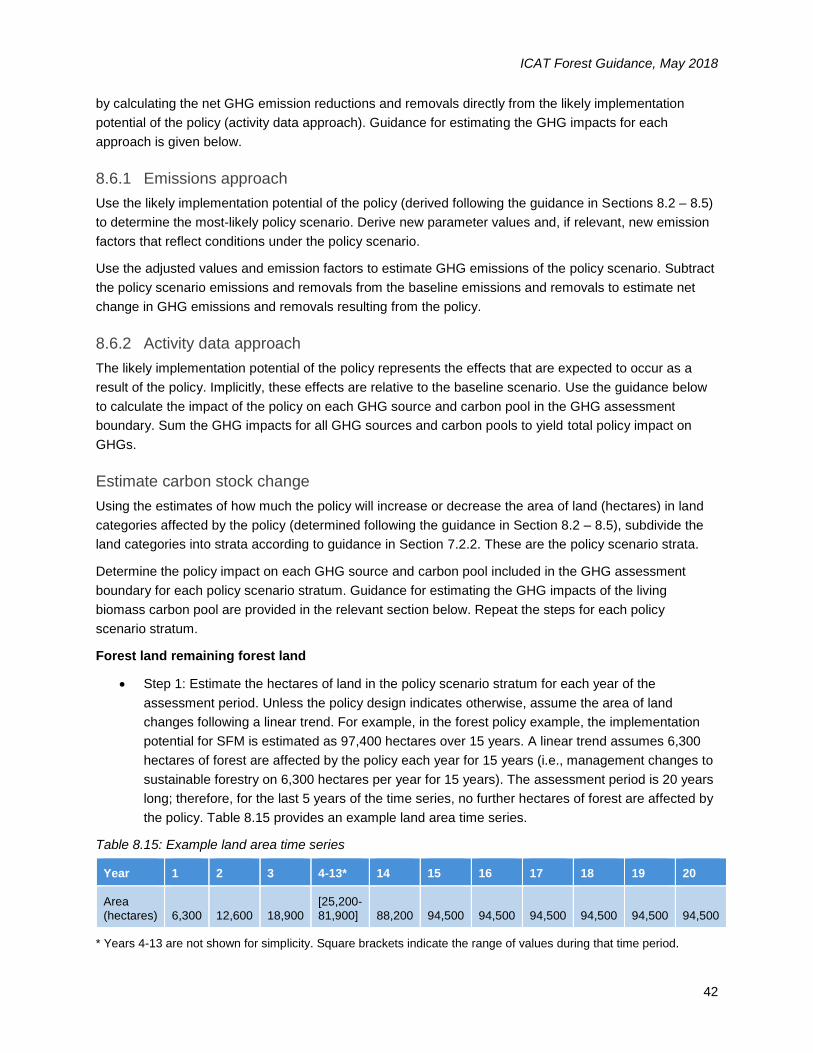
ICAT Forest Guidance, May 2018
42
by calculating the net GHG emission reductions and removals directly from the likely implementation
potential of the policy (activity data approach). Guidance for estimating the GHG impacts for each
approach is given below.
8.6.1 Emissions approach
Use the likely implementation potential of the policy (derived following the guidance in Sections 8.2 – 8.5)
to determine the most-likely policy scenario. Derive new parameter values and, if relevant, new emission
factors that reflect conditions under the policy scenario.
Use the adjusted values and emission factors to estimate GHG emissions of the policy scenario. Subtract
the policy scenario emissions and removals from the baseline emissions and removals to estimate net
change in GHG emissions and removals resulting from the policy.
8.6.2 Activity data approach
The likely implementation potential of the policy represents the effects that are expected to occur as a
result of the policy. Implicitly, these effects are relative to the baseline scenario. Use the guidance below
to calculate the impact of the policy on each GHG source and carbon pool in the GHG assessment
boundary. Sum the GHG impacts for all GHG sources and carbon pools to yield total policy impact on
GHGs.
Estimate carbon stock change
Using the estimates of how much the policy will increase or decrease the area of land (hectares) in land
categories affected by the policy (determined following the guidance in Section 8.2 – 8.5), subdivide the
land categories into strata according to guidance in Section 7.2.2. These are the policy scenario strata.
Determine the policy impact on each GHG source and carbon pool included in the GHG assessment
boundary for each policy scenario stratum. Guidance for estimating the GHG impacts of the living
biomass carbon pool are provided in the relevant section below. Repeat the steps for each policy
scenario stratum.
Forest land remaining forest land
Step 1: Estimate the hectares of land in the policy scenario stratum for each year of the
assessment period. Unless the policy design indicates otherwise, assume the area of land
changes following a linear trend. For example, in the forest policy example, the implementation
potential for SFM is estimated as 97,400 hectares over 15 years. A linear trend assumes 6,300
hectares of forest are affected by the policy each year for 15 years (i.e., management changes to
sustainable forestry on 6,300 hectares per year for 15 years). The assessment period is 20 years
long; therefore, for the last 5 years of the time series, no further hectares of forest are affected by
the policy. Table 8.15 provides an example land area time series.
Table 8.15: Example land area time series
Year 1 2 3 4-13* 14 15 16 17 18 19 20
Area
(hectares)
6,300
12,600
18,900
[25,200-
81,900]
88,200
94,500
94,500
94,500
94,500
94,500
94,500
* Years 4-13 are not shown for simplicity. Square brackets indicate the range of values during that time period.
ICAT Forest Guidance, May 2018
43
Step 2: Calculate the annual carbon stock change for living biomass for the policy scenario
stratum based on the land area time series estimated in Step 1 and the guidance in Section 7.2.4
for forest land remaining forest land. Call this term ∆𝐶𝐵𝑖𝑜𝑚𝑎𝑠𝑠_𝑤𝑖𝑡ℎ 𝑝𝑜𝑙𝑖𝑐𝑦 (units are tonnes C/year).
Step 3: Determine the baseline scenario stratum, which is the most likely stratum if the policy
were not enacted (without policy). The ecological zone in the baseline stratum should be the
same as in the policy scenario stratum. The management category should be different from the
policy scenario stratum. The baseline land area time series is identical to the policy scenario land
area time series developed in Step 1 because it represents the same land as the policy scenario
under an alternative scenario. Calculate the annual carbon stock change in living biomass for the
baseline stratum based on the land area time series estimated in Step 1 and following the
guidance in Section 7.2.4 for forest land remaining forest land. Call this term
∆𝐶𝐵𝑖𝑜𝑚𝑎𝑠𝑠_𝑤𝑖𝑡ℎ𝑜𝑢𝑡 𝑝𝑜𝑙𝑖𝑐𝑦 (units are tonnes C/year).
Step 4: Calculate the cumulative carbon stock change over all years of the assessment period,
separately for the baseline and policy strata.
Step 5: Subtract the baseline cumulative carbon stock change from the policy cumulative carbon
stock change to yield the policy impact on the living biomass carbon pool for the land strata.
Non-forest land converted to forest land
Step 1: Estimate the cumulative hectares of land in the policy scenario stratum for the
assessment period. For example, in the forest policy example, it is estimated that 14,250
hectares of cropland will be converted to forest land through general tree planting as a result of
the policy. Therefore the cumulative hectares of land in the policy scenario stratum for non-forest
land converted to forest land is 14,250 hectares.
Step 2: Calculate the change in forest carbon stocks from land conversion using Equation 7.1 in
Section 7.2.4. Set the area term in Equation 7.1 equal to the hectares of land from Step 1. This
yields the policy impact on the living biomass carbon pool for the land stratum.
Reduced forest land conversion to non-forest land
Step 1: Estimate the cumulative hectares of land in the policy scenario stratum for the
assessment period. For reduced deforestation, this will be the estimated amount of forest land not
converted to non-forest land as a result of the policy.
Step 2: Calculate the change in forest carbon stocks from land conversion using Equation 7.1 in
Section 7.2.4. Set the area term in Equation 7.1 equal to the hectares of land from Step 1.
The result of Equation 7.1 will be the estimated carbon stock loss that would have occurred if
those hectares were deforested. Multiply the result of Equation 7.1 by -1 to convert the outcome
to carbon stock gain because the policy reduced this amount of forest carbon stock loss. This
yields the policy impact on the living biomass carbon pool for the land stratum.
8.6.3 Calculate GHG impacts
Calculate the total policy impact on the living biomass carbon pool by summing the results for all policy
scenario strata. Convert the net carbon stock change to GHG emission reductions or removals,
expressed as tonnes of CO2e, by multiplying by 44/12 and -1. This generates the cumulative policy

ICAT Forest Guidance, May 2018
44
impact in terms of tonnes CO2e emissions (positive) or removals (negative). Divide the cumulative policy
impact by the number of years in the assessment period for the annual GHG impacts of the policy.
Where other GHG sources and carbon pools are included in the GHG assessment boundary, calculate
their impact in terms of CO2e emissions and add to the policy impact on the living biomass carbon pool.
ICAT Forest Guidance, May 2018
45
ESTIMATING GHG IMPACTS EX-POST Ex-post impact assessment is a backward-looking assessment of the GHG impacts achieved by a policy
to date. The GHG impacts can be assessed during the policy implementation period or in the years after
implementation. Ex-post assessment involves evaluating the performance of the policy, and estimating
the impact of the policy by comparing observed policy scenario values (based on monitored data) to ex-
post baseline values. In contrast to ex-ante assessment, which is based on forecasted values, ex-post
assessment involves monitored or observed data collected during the policy implementation period. The
impact of the policy (ex-post) is estimated by subtracting baseline estimates from policy scenario
estimates. Users that are estimating GHG impacts ex-ante only can skip this chapter.
Figure 9.1: Overview of steps in the chapter
Checklist of key recommendations
Estimate or update baseline emissions using observed values for parameters that are not affected
by the policy and estimated values for parameters that are affected by the policy
Ascertain whether the inputs, activities and intermediate effects that were expected to occur
according to the causal chain, actually occurred (if relevant)
Estimate the GHG impacts of the policy over the assessment period for each GHG source and
carbon pool included in the GHG assessment boundary
Estimate or update baseline emissions
It is a key recommendation to estimate or update baseline emissions using observed values for
parameters that are not affected by the policy and estimated values for parameters that are affected by
the policy. The baseline emissions can be estimated following the guidance in Section 7.2. Further
guidance on monitoring parameters is provided in Chapter 10. The baseline and policy scenarios have
the same GHG assessment boundary.
Where the baseline scenario was determined and baseline emissions estimated in a previous ex-ante
impact assessment, this should be updated by replacing estimated values with observed data for non-
policy drivers.
Estimate GHG impacts
Evaluate performance of the policy (if relevant)
The performance of the policy should be evaluated to ensure that the GHG impacts calculated ex-post
can be attributed to policy. To do this, it is a key recommendation to ascertain whether the inputs,
activities and intermediate effects that were expected to occur according to the causal chain, actually
Estimate or update baseline emissions
(Section 9.1)
Estimate GHG impacts
(Section 9.2)
ICAT Forest Guidance, May 2018
46
occurred. For ex-post impact assessments where no previous ex-ante assessment has been conducted
this step can be skipped.
Chapter 10 provides examples of the inputs and activities that should be monitored to evaluate the
performance of the policy. If the user cannot ascertain that the inputs or activities occurred, it is not
possible to attribute GHG impacts to policy implementation.
Users should also examine whether the intermediate effects in the causal chain occurred. It may not be
feasible to monitor all intermediate effects. At minimum, each of the intermediate effects linked to GHG
sources and carbon pools included in the GHG assessment boundary should be monitored with at least
one parameter. Table 6.2 and Table 6.3 in Chapter 6 provide examples of intermediate effects that should
be monitored. If the user cannot confirm that these intermediate effects occurred, it is not possible to
attribute GHG impacts to policy implementation.
Note that inputs, activities and/or intermediate effects may be lower or higher in magnitude than expected
but this does not mean that GHG impacts cannot be attributed to the policy.
Estimate the GHG impact of the policy
It is a key recommendation to estimate the GHG impacts of the policy over the assessment period for
each GHG source and carbon pool included in the GHG assessment boundary. The same methods used
to estimate baseline emissions should be used to estimate policy scenario emissions to allow for
meaningful tracking of performance over time.
Calculate policy scenario emissions using the estimation methods provided in Section 7.2. Use observed,
measured or recently collected activity data, and measured or re-estimated emission factors. Further
guidance on monitoring parameters is provided in Chapter 10.
If using the emissions approach, calculate the GHG impacts of the policy by subtracting baseline
emissions (estimated in Section 9.1) from the ex-post policy scenario emissions for each GHG source
and carbon pool included in the GHG assessment boundary.
If using the activity data approach, calculate the GHG impact of the policy directly, by determining the
actual implementation level using observed, measured, or recently collected data and measure or re-
estimate emission factors. It is not necessary to estimate the GHG emissions of the baseline scenario
when using this approach. Rather, users should follow the guidance in Section 8.6.2 using ex-post activity
data and emission factors. Under this approach, users should carefully consider the policy’s inputs,
activities and intermediate effects that occurred ex-post as a result of policy. Users should report and
justify that the actual implementation level (e.g., the observed change in activity data) is the result of the
policy.