Forest Economics

© Peter Berck 2008,2013, 2014

Forest class notes on Linear Programming and Forests

The Basic Model of Forestry

The control variable is a treatment, a complete harvest is the one we will examine.

Other treatments include Partial harvest or thinning Fertilizing (pays in Sweden) Clearing understory with fire

Objective

We examine Net Present Value Foresters are trained to ask about the

(usually multiple) objectives of owners. Examples: Estate tax payment so as to allow a long

term ownership to continue. (Sweden) Environmental or Aesthetic Water, Wildlife (hunting), visual buffer,

etc.

Time conventions and cut

Type of Site, j: soil, tree species, altitude, etc Many “birthdays”

First is –M. : That is today is day zero. hj(t,s)

t is calendar time s is birthday of stand; t-s is therefore age h is acres harvested

Dj(t-s) is volume per acre

Present value of cut

v(t) is cut at t from all stands and ages V(t) =j s>=-M Dj(t-s) hj(t, s) P(t) is price of standing trees at time t,

called the stumpage price Present value is

( )( ) ( ) ( ) 1

s t

s t

PV t P s V s r

Conservation of acres

Initial Acres = Acres cut over all time Aj(s) = t>s hj(t,s)

s is birthday

Recall: h(current time, birthday)

A(s) are the initial conditions

Cut acres at t re-grow and are recut at a > t s hj(t,s) = a hj(a,t)

Cut at t from all birthdays (s<=t) is what is reborn at t and therefore cut in times a>t.

This is where bio differs from fish.This is Johnson and Scheurman, Model II.

Full Problem

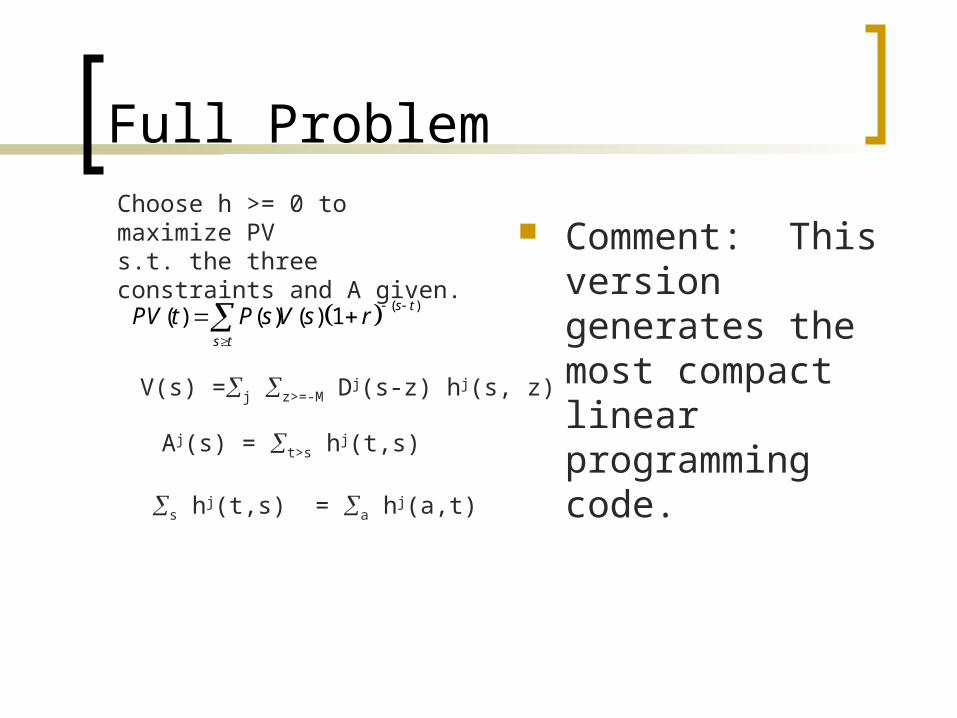
Comment: This version generates the most compact linear programming code.

( )( ) ( ) ( ) 1

s t

s t

PV t P s V s r

V(s) =j z>=-M Dj(s-z) hj(s, z)

Aj(s) = t>s hj(t,s)

s hj(t,s) = a hj(a,t)

Choose h >= 0 to maximize PVs.t. the three constraints and A given.

Easier to understand and program

Add another variable, x(t,s) the number of acres standing at time t of land regenerated at time s.

x is what is left standing at z from stands born in s <= z

x(time, birthday)

xj(z,s) = Aj(s) - t<Z hj(t,s) For stands born before time zero s< 0, A(s) is given. For stands born at zero or later. Let Aj(s) = a hj(s,a)

What is left at time z from what was born at time s = what there was to start, A, less what was cut up till now=time z.

Compact Set Up

The same problem explicitly as an LP in matrix form.

We reduce the number of stands to one, which is fine until there are constraints between stands.

Easier to use x as a vector

Originally we had x(t,s) We find it easier to use Xt=(x(t,t),x(t,t-1),….x(t,t-n-1))’ That is X is now a vector of acres by

age class. We also make n-1 the oldest possible acres.

In what follows A will NOT be the A from before—sorry!

A LP One Stand Example

1 1 1 1

1

0 0 1 1 1 1 1

. . . .1 0 0 0 0

. . . .1

. . . .1

1 1 0 0n n n nt t t t

x x h h

x x h h

X(t+1) =< A(X(t) – h(t)) +Bh(t)= Ax(t) +(B-A) h(t) All in acres.

Stack em: 3 periods

1

2 1

3

1

2

*

0

0

x

xI x

xA I B A

hA I B A

h

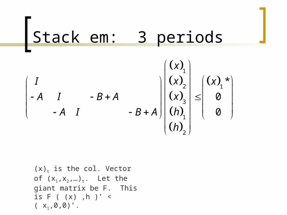
(x)t is the col. Vector of (x1,x2,…)t. Let the giant matrix be F. This is F ( (x) ,h )’ < ( x1,0,0)’.

Stack em: 3 periods

1

2 1

3

1

2

*

0

0

x

xI x

xA I B A

hA I B A

h

F z ≤b

Expanded Objective Function

Let E(s,t) be value of wildlife, etc Y(t) = j s>=-M Dj(t-s) hj(t, s)P(t) +

j s>=-M xj(s,t) Ej(s,t)

Max present value of Y(t).

Objective

/ (1 ) where D is the volume in age class i

E is the value of stock in class i at time t, e.g. for

carbon or spotted owls

G is the vec(G ) and E is vec

max ' ' subject to constra

tit i t

it

it it

G D P r

E

E x G h

ints on

previous slide and x,h 0

LP

Let F be the giant matrix and c be the vector of E’s and G’s Let z = (x,h) and b= (x*(1),0…0)’ ( a ‘ is a transpose)

Max c’z s.t Fz ≤ b (x(1),0…0)’ primal A result from LP is that an equivalent

problem is Min b’ s.t. F’ ≥ c dual

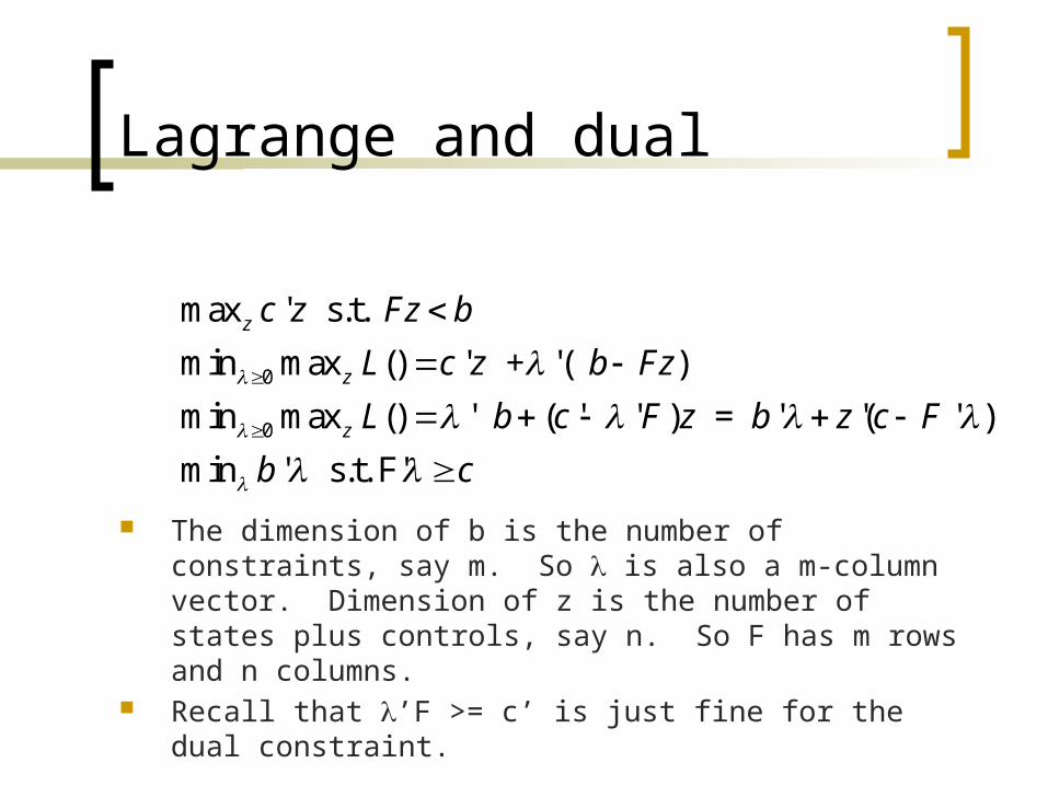
Lagrange and dual

The dimension of b is the number of constraints, say m. So is also a m-column vector. Dimension of z is the number of states plus controls, say n. So F has m rows and n columns.

Recall that ’F >= c’ is just fine for the dual constraint.

0

0

max ' s.t.

min max () ' + '( )

min max () ' ( ' ' ) = ' '( ' )

min ' s.t. F'

z

z

z

c z Fz b

L c z b Fz

L b c F z b z c F

b c

Writing out our probelm

Lets cut this down to size: 3 periods and 3 age classes. So x is just born, one year old, two (or more) years old.

Write out problem and dual. Solve dual for a simple rule. Sketch below

Steps

Write out A and B for 3 age classes. What are the dimensions of A and B?

What are the dimensions of F? I count 9 constraints, one for each age class in

each time period. Group your so that ()1=(age=1,

time=1, a=2, t=1, a=3, time=1). Group your c’s the same way. Recall that the first 3 c’s are the value of

standing stock and the last two the value of harvest.

Using your neat new notation

Write out ’F >= c’ in terms of the A’s and B’s. You should have 5 matrix equations.

.

Dual

One can show that the dual to the simple problem is:

Max( value of cutting, value of leaving alone) Cutting is just Dj(t-s) P + shadow of bare

land at t. Leaving stand is shadow of land one

period older next period.

Expanding the model

When to cut with more constraints?

How much old timber to hold? Costs of not profit max policies

Like don’t cut till CMAI (top of growth curve)

Like hold onto oldgrowth for a while Like have a nondecling flow of timber National Forest Management Act.

More meaning to the model

Types of sites, j different species site classes critical locations

near streams visual buffers

More Constraints Don’t cut type j Keep N% of

forest at age, t-s, > 100

More treatments commercial thin pre-commercial

thin

Biology

Could use stand table. McArdle Bruce Meyer tables for doug fir

Could use stand simulator and then table the results

Must handle changes in stand discretely—possibly as stand with new growth function—eg. After fertilize

This JS model was basis for huge planning exercise for national forests.

Required by RPA (Resources Planning Act of 1974)

Hampered by large numbers of additional constraints on types of land that could be cut and when.

Eventually died of its own weight.

Stochastic

Can be turned into stochastic program. Dixon and Howitt do this by taking linear quadratic approximations and solving them. (AJAE)

Fire, insects, make stochastic advisable if planning is objective.

Valuing stock

Easy: Just add terms to the objective function of the form

X E Where X is stock and E is value Dual now includes added term in E This formulation takes care of carbon

sequestration.

Carbon

Imagine adding 1t co2e to the stock in the DICE model and finding the change in value. That is the price of carbon for each time.

Now imagine cutting a tree and having it release carbon over time while its replacement is growing.

There will be a delta for each time. Got to multiply by the shadow value.

Example:

Price of co2e: 10, 15, 20 in 3 decades.

Cut 1 ton co2e tree in first decade, 20% goes back to atmosphere each decade.

Growth is 2., .3 , .4 tons Net is 0, .1, .2 tons; Hence +$ 5.5 Need to do this over a very long time

to get it right.

Example 2

Plant a forest that burns after 30 years. P = 10, 20, 30. Growth .2, .3, -.5 Does this make you wonder about

what the prices must really mean? Perhaps clearer if rental rate: take out

one unit co2e in yr 1 and put it back in year 2.

Turning JS into a estimating model

Want to know if private and public forest were managed differently and if so what was “optimal” or what the shadow losses were of public management.

Need to estimate future prices and appropriate interest rate.

Hotelling: Derivative of profit function is supply.

( ) ( ) where Q is demand curve.p

CS P Q z dz

How do we get P

Model of previous section has value function J(P1,…,Pn, r) where P are the prices in the n periods and r is the interest rate.

Let CS(Pi) be consumer surplus of i Consider functional Z(P,r) = J + S

CS(Pi) Function takes a minimum where

supply = demand (2nd deriv positive)

Demand

Demand is estimated from time series data. Price and housing starts are most important variables in demand

Forest stock identifies the demand equation.

Now– for each choice of r, using the rule that P mins Z we can find P(r)

Given the Prices, the planning part of the model gives the cut, h.

Residual is predicted less actual cut Min sum sq. resids by varying r This estimates the model

Given the r and the P’s it is a simple matter to value the losses to cmai (small) and to oldgrowth retention, large.

Forest Area/Deforestation

US: Virgin forest to today: less forest

However NE and S. both regrew Large parts of rural US are going back to

forest General trend is for less forest Foster and Rosenzweig look at India

Naïve

Many LDC’s have insufficient land ownership to protect forests Marcos denuded the Phillipines for profit Nepal has problems with marginal ag

taking over forest regions

India

Gross forest statistics like US Area goes down Then up

Why? Market stories require property rights—

FR implicitly assume such. Demand for forest products goes up,

forests should go up. Long run, true Short run could go other way. Not so obvious

FR

Interest is the in the matched dataset of sattelite imagery (historical forest cover) to village surveys.

Find that increased population or expenditure on forest products leads to more forest land.

Wages, ag land prices insignificant New England can be told with wages or time to

regenerate Need relative ag land/ forest land price to do this

in the normal way Also need the product price for forest, don’t have

plausible that more income = more forest

Carbon

Carbon sinks include soil and trees From Sohngen and Mendelson

10% more carbon could be sequestered in forests Either more land Or more intensive management

Unclear how one would keep it tied up in soil or trees

$1-150 per ton are estimates for sequestration

Optimal

To decide what to do need to know the value of carbon sequestration by time period.

S-M model Damage function of carbon stock dStock/dt = emissions – abatement Reducing emissions and abatement are

costly Minimize present value of costs

soln

There is a shadow price of carbon, the marginal value of reducing the stock by one unit. Marginal costs = that

Problem: forestry stores the carbon for a while. Uses rental rate for carbon Interest on value less Price increase Worth investigating==might not be right

Empirical

Melds forest and climate model Gets price for emissions abatement Finds how sequestration changes land

and forest prices Finds equilibrium with higher prices for

forest land (bid up because of sequestration)

Sequestration makes sense, but is less profitable than with no price rise

Other subjects

Employment Trade (and the Lumber Wars) Private non industrial supply Mean reversion of prices Diversity and the need for large

untouched blocks vs. diversity in cut areas

Steps

1. write out the dual constraints, all 5 of them.

2. What is lambda(3)? 3. Now work backwards and get the

other two Remember x and lamda are non-

negative. Also need to make lamda small says the objective function