Forensic Geoscience Database By Richard Hudson · PDF file2.1 Soil Formation iiiiiiivv There are fives important forces that when combined form soil; these are climate, organisms,

A

Forensic Geoscience Database By

Richard Hudson

This watermark does not appear in the registered version - http://www.clicktoconvert.com

http://www.clicktoconvert.com

B

An understanding of the properties and laboratory methods for analysing soil were developed

to aid data analysis. Sample Data was retrieved and analysed to identify soil properties with

high distinguish-ability. The results of this data analysis were used in cohesion with user

demand to establish requirements for a prototype capable of matching a soil sample with the

most probable site the sample came from. The design and implementation of the prototype

were conducted synchronously to establish a working prototype. The prototype was evaluated

to provide future recommendation for the development of further prototypes or a fully

functional system.



C

Table of contents

1. Project Aim 1

1.1 Problem 1

1.2 Problem Owner 1

1.3 Intended Users 1

1.4 Deadline 1

2. The Nature of Soil 2-5

2.1 Soil Formation 2

2.2 Soil Horizons 2-3

2.3 Soil Classification 3

2.4 Soil Maps

3

2.5 Data Gathering and Laboratory

Techniques

3-5

2.51 Gathering the Soil 3

2.52 Methods of Analysis 4

2.521 X-Ray Fluorescence Spectrometry 4

2.522 Loss on Ignition 4

2.523 Soil PH in Water

4

2.524 Soil Carbonate 4

2.525 Chromatography (Colour Analysis) 4-5

2.526 Grain Size 5

2.527 Moisture Content

5

2.6 Forensic Use of Soil 5

3. Data Acquisition

6-9

3.1 Pre-arranged Data

6-7

3.11 Source

6

3.12 Soil Sampling 6

3.13 Grid Coordinates and Location Soil

Type

6-7



D

3.14 Laboratory Methods 7

3.2 Important Methods of Analysis

Indicated by Independent Studies

7-8

3.3 Ideal Data

8

3.4 Issues Surrounding Data 8-9

4. Data Analysis

9

4.1 Introduction

9

4.2 Sample Issues

9-10

4.3 Establishing Distinguish-ability of Soil Properties

9-20

4.31 Soil PH in Water 10

4.32 Soil Carbonate 10-11

4.33 Loss on Ignition

11-12

4.34 X-ray Fluorescence Spectrometry

12-16

4.35 Chromatography 16-20

4.4 Matching

20-26

4.41 Analysis

20-25

4.42 Probable Vs. Actual

25-26

5. Project Management

26-28

5.1 Initial Schedule 26-27

5.11 Performance

26-27

5.12 Major Factor Influencing Performance 27

5.2 Schedule Amendments 26-27

5.21 Amendments

27



E

5.22 Major Factor Influencing

Amendments

27

5.23 Indication of Success

28

5.3 Review Schedule Performance 28

6. Requirements Specification 28

6.1 Requirements Capture Techniques

28

6.2 Techniques Used

28-29

6.3 Overview of Information Collected 29-30

6.31 Functional Requirements

29

6.32 Non- Functional Requirements 29-30

6.33 Use Case Diagram

30

6.4 Requirements List 30-33

6.5 Prototype Minimum Requirements 33-34

6.6 Software 34-35

7. Design/ Implementation 35-38

7.1 Introduction 35

7.2 Data Structure 35-36

7.3 Input 36

7.4 Data Analysis

37

7.5 Output 37-38

7.6 Interface 38

8. Evaluation 39-45

8.1 Testing and Performance 39-43

8.11 Introduction 39

8.12 Test List: Predicted Vs. Actual Results

39-41

8.13 Functional Performance 41-42

8.14 Non-functional Performance 42-43

8.15 User Response 43



F

8.151 Training Schedule (15 minutes)

43

8.152 Interview and Observation of User 43

8.2 Recommendations 44-45

Appendices I -XLIV

Appendix A I

Appendix B. II-VIII

Appendix C IX-XIV

Appendix D XV-XVII

Appendix E XVIII-XX

Appendix F XXI-XXII

Appendix G XXIII

Appendix H XXIV-XXV

Appendix I XXVI-XXVII

Appendix J XXVII

Appendix K XXVIII

Appendix L XXVIII

Appendix M XXIX

Appendix N XXX

Appendix O XXX

Appendix P XXX-XXXI

Appendix Q XXXI

Appendix R XXXI-XXXII

Appendix S XXXII-XXXIV

Appendix T XXXV

Appendix U XXXV

Appendix V XXXVI-XLIV

Bibliography G-H



1

Forensic Geoscience Database

1. Project Aim

1.1 Problem

Produce a demonstrator capable of matching a soil sample with a database holding site

information to determine the most probable site the sample came from.

1.2 Problem Owner

Robert Mortimer a lecturer of Environmental Geochemistry in the Earth Sciences

Department. He holds an interest in which measurements and associated statistical techniques

identify the most reliable match between a soil sample and source site. He requires a solution

to the problem for his intended users.

1.3 Intended Users

The users will be students from the Earth Sciences Department that partake in Robert

Mortimer’s Environmental Geochemistry modules. The students will conduct field studies

that capture soil sample information. This data will be entered into a system that will store

and manipulate the data and attempt to match it to data stored in the system, and output a

credible source site, which they can verify or dismiss.

The solution may be presented to the West Yorkshire Police as an illustration of the forensic

use of soil analysis in solving crime.

1.4 Deadline

28th

April 2004



2

2. The Nature of Soil

2.1 Soil Formationiiiiiiivv

There are fives important forces that when combined form soil; these are climate, organisms,

relief, parent material and time.

The main components of climate are moisture and temperature. The climate affects mineral

weathering and controls the vegetation cover. Organisms includes vegetation, the animal life

in the area, microorganisms and man. Relief is the major topography features (i.e. slope and

aspect). Properties of the parent material that influence soil development include, mineralogy,

composition and texture. Time may influence soil formation in two ways, firstly, soil-forming

factors may vary over time, and secondly, more time may result in further soil transformation.

It is apparent that although evaluated independently, they all interlink to form soil.

2.2 Soil Horizonsviviiviii

When soil is examined, it can comprise of six layers that represent its form at various depths.

The depth of these layers will depend on location. These layers are known as master horizons,

which themselves can be subdivided into specific unique layers.

The topmost horizon is generally the Organic Horizon that consists of fresh decaying plant

residue (i.e. leaves, twigs, moss, etc…). The dark colour of this horizon is a product of the

formation of this partially decomposed organic soil material.

The Top Soil/ Surface Horizon is beneath the Organic Horizon and largely consists of mineral

material. This horizon is usually the most productive layer of soil due to the occurrence of root

activity. It contains larger quantities of decomposed organic matter than other layers of soil;

hence this is a darker colour than the Organic Horizon.

The Sub-surface Horizon follows the Top Soil Horizon and its main feature is the loss of

partially decomposed organic soil material, iron, aluminium and silicate clay leaving a

concentration of silt or sand particles, resulting in a beached white-ish colour. The water that

moves down through this layer is responsible for soluble minerals and nutrients dissolving.

The Sub-Soil Horizon falls under the Sub-surface Horizon and is generally the level that

washed (water passing through Sub-Surface Horizon removes soluble minerals and nutrients)

materials accumulate. It is often lower in organic matter, denser and lighter in colour to the

Top Soil Horizon.

The fifth layer is the Substratum Horizon/ Parent Material, which is a combination of partially

disintegrated parent material and mineral particles.

The lowest Horizon is bedrock.



3

2.3 Soil Classification

It is important to classify soils so that properties may be remembered and relationships

between groups may be understood. Soil classification helps reduce complexity as it helps

organise and simplify soil profiles into soil classes (AKA soil series).

There are two main approaches to soil classification either natural or technical classification.

Natural classification uses intrinsic properties or behaviour of soil as a basis for classification.

Whereas technical classification is more focuses on grouping soil according to use.

The Soil Classification used in England and Wales is that of Avery (1973)ix. This is a natural

classification that consists of ten Soil Groups differentiated by general soil profiles

characteristics according to the arrangement and type of soil horizons. The Soil Groups are

divided into forty-three Groups dependent on the existence of decisive horizons and

composition of soil materials. The Groups are divided into one hundred and three Sub-groups,

again with reference to diagnostic horizon and composition. At the lowest level of abstraction

the Sub-groups are divided into Series that are distinguished according to mineralogy, origin,

texture and profile contrast.

2.4 Soil Maps

A soil map is a map of a designated area that illustrates soil type and its boundaries according

to a soil classification at a specific level of abstraction. For example, a low detailed map may

use Avery’s Soil Groups, where as a highly detailed map may use Avery’s soil series. The

soil types are indicated by a legend. A soil map is usually supplemented with a notebook that

explains the procedures used for soil classification.

2.5 Data Gathering and Laboratory Techniques

2.51 Gathering the Soil

This is usually done manually using a trowel, which is a flat, pointed metal tool with a handle

that allows the geologist to delicately dig and scrape away at layers of matter. A soil pit can

also be dug with the aid of an Auger Boring Machine that is a complex piece of drilling

equipment.

2.52 Methods of Analysis



4

2.521 X-Ray Fluorescence Spectrometry

This method is a form of spectroscopy (“The technique of observing the spectra of visible light

from an object to determine its composition, temperature, density, and speed”x), which is

perfect for the quick and easy measurement of elements within a material. For example, a

XRF Spectrometer could determine the major elemental compositions of a soil sample.

2.522 Loss on Ignitionxi

Loss on Ignition is a method commonly used to establish the organic and carbon content of

sediment. For example, a sample of soil will be weighed before it is ignited (100% weight).

Then put into a furnace at a standard temperature of 1025oC removing residue leaving carbon

and organic content that is expressed as a percentage of the original weight using the

following calculation:

LOI = (sample weight – residue weight) X 100

Sample weight

2.523 Soil PH in Water

This method involves adding a sample of soil to water and mixing the ingredients, which are

tested for a level of PH (“a logarithmic scale used to describe the acidity or alkalinity of a

solution. Water has a neutral pH of 7. A pH below 7 is acidic; a pH above 7 is alkaline”xii

).

2.524 Soil Carbonate

This is a method that enables the carbonate (“a compound containing carbon and oxygen”xiii

)

content of sediment to be calculated in terms of weight.

2.525 Chromatography (Colour Analysis)xiv

A spectrophotometer (“an instrument that measures the amount of light a colour sample

reflects or transmits at each wavelength, producing spectral data”xv

) is used to measure

colour values of sediment, using integrated sphere geometry to produce a numerical

specification for an individual colour.

Colour can be described using three basic components hue (actual colour of an object),

lightness and chroma (vividness/ dullness). The numerical specification of a colour can be

described on its coordinates within a 3-D scale. Where the x-axis represents red (positive) to



5

green (negative), y-axis represents black (position 0) to white (position 100), and the z-axis

represents blue (negative) to yellow (positive).

The x, y and z coordinates are represented by a*, L* and B* respectively (lightness). There

are Polar coordinates C* (chroma – coordinates (x, y)) and h* (hue angle = tan-1 (b*/a*)).

These values are produced by measuring the amount of light of each wavelength reflected by

an object.

2.526 Grain Size

This method involves calculating an average for the grain size of sediment.

2.527 Moisture Content

Moisture content is calculated by weighing sediment before and after it has been dried to

establish a difference, which is the weight for the moisture.

2.6 Forensic Use of Soil

The forensic use of soil is part of the forensic geology branch of forensic science. Forensic

geology is still at a relatively infant stage of its development, even though it can be traced

back as far as 1887 in the literary works of Sherlock Holmes.

However its use is evidently growing and its importance in crime prevention and resolution is

unquestionable. Soil is just one of many geological materials that is used to solve or prevent

crime. Its common use is to examine two soil samples and identify that they have a common

source. “We cannot overestimate the value of finding artefacts in the soil, such as manmade

objects or chemicals or types of evidence such as paint or fibre fragments”xvi

. For example, in

the scenario of a ‘hit and ‘run’ (a careless driver of a vehicle may hit another vehicle or

pedestrian and leave the scene of the accident without stopping) soil could be found on the

suspects vehicle and matched with the soil at the scene of the accident, hence providing

evidence of the suspects involvement.

The increase in soil analysis techniques with improved accuracy promotes more diverse and

conclusive use in crime prevention and resolution.



6

3. Data Acquisition

3.1 Pre-arranged Data

3.11 Source

The data was arranged before the project had begun with the problem owner Robert

Mortimer. He had two undergraduate students conducting a dissertation on “the feasibility of

using forensic techniques to identify soil types using samples from the West Yorkshire

area”xvii

. The data from the two students was promised once sampling and laboratory analysis

had been conducted.

3.12 Soil Samplingxviii

Nine locations were selected at random over the West Yorkshire area. Three samples were

taken at each location. The soil was gathered using a trowel digging to a 15cm depth. The

samples were frozen and freeze dried before laboratory analysis. The soil was collected on the

6th

June 2003 in dry weather conditions.

The problem owner selected three unknown locations and two samples were made at each

location. These samples were made for test purpose.

3.13 Grid Coordinates and Location Soil Typexviixviii

The coordinates for the locations are taken from Landranger Ordinance Survey Maps of

1: 50 000 scale. These coordinates were mapped onto a soil map (Soils of Northern England,

Soil Survey of England and Wales) of 1: 250 000 scale to establish Soil Type. It uses Avery’s

(1973) soil classificationix.

Location

No.

Location Name Ordinance

Survey Map

No.

Grid Coordinate

(6 figure)

Soil Type

1 Greenlands 104 (069, 204) 541f/g

2 Blackhead 103 (995, 278) 721c

3 Riddlesden 104 (091, 443) 721c

4 Warmfield 104 (383, 207) 713a



7

5 Walsden 103 (982, 201) 1011b

6 Widdop Reservoir 103 (916, 338) 1011b

7 Lindley Woods 104 (208, 498) 711p

8 Bramham 105 (444, 426) 511a

9 Kirkham Gate 104 (290, 240) 712a

3.14 Laboratory Methods

Matthew Bell gathered soil from location numbers 1, 2, 3 and 4, and David Granville sampled

soil from location numbers 6, 7, 8 and 9. Both students conducted X-ray Fluorescence

Spectrometry, Loss on Ignition, Soil PH in Water, Soil Carbonate and Chromatography

methods of analysis. Both used the same experiment design, which allowed the data

formulated from laboratory analysis to be combined.

David Granville also conducted Moisture Content and Grain Sizing methods of analysis. The

exact methods of analysis are documented within their dissertationsxviii

.

All laboratory analysis used freeze-dried soil sample, apart from Moisture Content analysis.

All of the methods of analysis were applied to the test samples. The data formulated from

analysis can be viewed in Appendix B.

3.2 Important Methods of Analysis Indicated by Independent Studies

A studyxix

conducted by Barry Rawlins and Mark Cave suggests that Chemical Analysis using

X-ray Fluorescence Spectrometry for small samples (as in forensic studies) would have

limited confidence in associating a soil sample with a site. This implies that a pinpoint

location cannot be made with full confidence, but the most probable site could be indicated. It

stipulates that Mn and Mg are the most powerful discriminatory elements. Simon Blott et alxx

indicate that when the analysis of soil grain sizing is combined with chemical analysis more

confidence can be established between matching soil samples.

Debra Croft and Kenneth Pye in their studyxxi

imply that the discriminatory power of colour

components of soil in establishing a match is excellent (95% confidence) when a

spectrophotometer is used to analyse colour 3-Dimensionally. It is also stresses that this

measurement can be made accurately on a very small sample.



8

The students have provided data induced from chemical, colour and grain sizing analysis that

will be the main focus of data analysis further in the report.

3.3 Ideal Data

It is indicated above that chemical, colour and grain sizing analysis are a good source for

discriminating between soil samples. Thus the provision of this data would be ideal, which is

provided by the students. However this data could mislead data analysis because the samples

are from a limited number of locations containing a wide range of soil types. Hence the data

is not ideal for conducting data analysis to distinguish between different locations for the

same soil type. It would be more affective to have gathered soil from more locations over a

smaller area covering fewer soil types.

Although the students provide chemical analysis, it does not identify single elements, only

compound element. The study on chemical analysis identifies the success of single

discriminating elements (i.e. Mn, Mg, Rb, Sr, Ni and Zrxix

). Thus it would be ideal to conduct

a finer chemical analysis.

There is an inaccuracy with the mapping of location coordinates to the soil map, because of

the difference between the map scales, so it would have increased accuracy to use maps of the

same scale.

3.4 Issues Surrounding Data

The pre-arranged data was neither ideal nor provided on time. Investigation into alternative

data sources was conducted throughout the Christmas break until early February.

It was sought to find data that was gathered from more locations over a smaller area

complying with suggested methods of analysis.

The search started by contacting the Geography Department within the University of Leeds to

arrange a meeting to discuss data acquisition with the appropriate personnel. Pippa Chapman

was the first point of contact and provided a data set for a hill slope in Skipton. This data set

did not contain chemical or colour analysis and was over a too small (1 mile square) area, so

was disregarded.

The British Geological Survey was contacted to enquire about what data sets they could

provide. Anthea Brown replied to the enquiry stipulating that the data was not readily

available from this source. It was recommended to try and contact the National Soil Resource

Institute based at Cranfield University. The National Soil Resource Institute did not respond

to enquiries that were made.



9

Pippa Chapman was contacted again to investigate whether she had any colleagues that may

hold relevant data sets. Lorna Dawson was an ex-colleague of Pippa Chapman working at

Macaulay Land Use research Institute in Aberdeen. Although the data set would not be from

the West Yorkshire area it was thought that sample data and test data might be provided.

However although the data set offered met with requirements it was too expensive to

purchase, so was disregarded.

An on-line resource Digimap was found through the University of Leeds on-line library

facilities. It provided everything but soil set data.

The University of Leeds libraries were investigated to discover whether finer detailed soil

maps existed for the area of West Yorkshire. This would provide lower level soil

classifications, site information and data from its associated handbook. The student data could

then be used as test data. However the finer detailed soil maps did not cover the specific

locations that the students had sampled, and also the data associated with the different soil

types did not comply with the required methods of analysis. Hence this source was

disregarded.

This is just a sample of the vast research conducted that provided an insight into data

available but not attainable.

4. Data Analysis 4.1 Introduction

It is important to be able to distinguish between the sample locations that soil was retrieved

from and also to be able to match a soil sample from an unknown location a its most probable

source. This section reports on the distinguishability of measurements generated from the

sample locations and attempts to match 3 unknown soil locations to one of the 9 known

locations.

The data produced by X-ray Fluorescence Spectrometry, Loss on Ignition, Soil PH in Water,

Soil Carbonate and Chromatography analysis for locations 1 to 9 will be examined to identify

whether the locations are distinguishable from one another. The extent of this

distinguishability will be discussed where it exists. The data from Moisture Content and Grain

Size analysis will be omitted because it is not available for all 9 locations.

4.2 Sample Issues

The number of locations sampled and the number of points sampled at each location affects

the degree of significance that can be drawn from the data. The data used for analysis uses a



10

very limited number of sample locations and sample points at each location. The implications

of this factor limits applicability of conclusions to a larger sample population, but cannot be

avoided. Hence the distinguishability of analysis methods in this section will only be

discussed in terms of the data sampled.

4.3 Establishing Distinguish-ability of Soil Properties 4.31 Soil PH in Water The PH Level for 3 samples from each location was represented visually using a bar chart that

is illustrated below:

It is clear that locations 1, 7 and 8 can be uniquely identified using this measurement.

However this indicates that 2/3rd

of the locations cannot, thus this measurement possesses a

low level of distinguish-ability.

4.32 Soil Carbonate

The Carbonate Content for 3 samples from each location was represented visually using a bar

chart that is illustrated below:

Soil PH in Water for Sample Locations

0.00

0.50

1.00

1.50

2.00

2.50

3.00

3.50

4.00

4.50

5.00

5.50

6.00

6.50

7.00

7.50

8.00

8.50

1 1 1 2 2 2 3 3 3 4 4 4 5 5 5 6 6 6 7 7 7 8 8 8 9 9 9

Locations

PH

Lev

el

(5g

So

il/ 5

ml

H2O

)

PH



11

Carbonate Content for Sample Locations

0.0000

0.0500

0.1000

0.1500

0.2000

0.2500

0.3000

1 2 3 4 5 6 7 8 9

Locations

Ca

rbo

nate

Co

nte

nt

(g)

Carbonate

The graphical representation of this measurement demonstrates that Sample location 8 can be

distinguished. However the remaining 8 locations cannot be classified. Therefore this

measurement for this data set provides low distinguishability. It is important to note that there

is limited consistency within sample points at each location, perhaps because the sample is

too small (i.e. If a larger sample was taken this inconsistency may find stability).

4.33 Loss on Ignition

The percentage Loss on Ignition for 3 samples from each location was represented visually

using a bar chart that is illustrated below:



12

Loss on Ignition for Sample Locations

0.00

10.00

20.00

30.00

40.00

50.00

60.00

70.00

80.00

90.00

100.00

110.00

1 1 1 2 2 2 3 3 3 4 4 4 5 5 5 6 6 6 7 7 7 8 8 8 9 9 9

Locations

Pe

rce

nta

ge

LOI

Average

This measurement enables all sample locations to be classified. The strength of this

classification is unclear, because only 3 sample points for each location were examined (i.e. if

there were more sample points present, overlap between the percentage Loss of Ignition for

the locations may exist).

4.34 X-ray Fluorescence Spectrometry

The average chemical composition for 3 samples from each location was represented visually

using a staked-column chart that is illustrated below:



13

The Average Chemical Composition for Sample Locations

0

10

20

30

40

50

60

70

80

90

100

1 2 3 4 5 6 7 8 9

Locations

Perc

en

tag

e

siO2 TiO2 Al2O3 FeO3 Mn3O4 MgO CaO Na2O K2O P2O5 Cr2O3

The graph demonstrates that the chemical compositions of the samples from the 9 locations

are unique. The extent was investigated by examining each individual element. Bar Charts

(see Appendix C) were constructed to demonstrate whether locations had a distinguishable

range of quantity of each element or otherwise. It is important to note that location 5 had a

high percentage Loss on Ignition, so most elemental compositions are highly distinctive. Also

the accuracy of any comparisons with location 9 may be inaccurate, because only 1 sample

point was provided. The results are noted in the underlying table:

Elemental Composition

Locations Distinguished

Overlap Between Sample Point Ranges (Locations) Notes

SiO2 3, 5, 6, 8, 9 1:2:4:7

Locations 5 and 9 are the most identifiable from this composition. The distinctiveness of location 6 is not certain because its range of sample points are relatively very close to those of location 4.

TiO2 3, 5, 6, 8 1:4, 1:9, 2:7

Locations 5 and 8 are the most identifiable from this composition. The ranges of sample points for locations 3 and 6 are very close, which suggest that if more samples points were taken overlap may exist. Alternatively if the measurements for this composition were taken to more than 2.d.p.’s the ranges may more distinctively classify the locations.



14

if the measurements for this composition were taken to more than 2.d.p.’s the ranges may more distinctively classify the locations.

Al2O3 1, 5, 6, 8 2:7, 4:9

It is uncertain whether location 2 and 9 ranges of sample points overlap, as only 1 sample point is present for location 9 and the ranges are very close.

Fe2O3 1, 3, 5, 6, 8, 9 2:4, 4:7

It is uncertain whether location 8 and 9 ranges of sample points overlap, as only 1 sample point is present for location 9 and the ranges are very close. The range of sample points for locations 3 and 6 are relatively close, thus gathering further sample points may provide warranted validation.

Mn3O4 1, 2, 4, 5, 7 3:6, 3:8, 3:9

Location 7 is the most identifiable from this composition. The sample point ranges for locations 1, 2 and 5 are very close and could been more confidently distinguished if measurements had been taken to further decimal places. The same is true of locations 4 and 6.

MgO 3, 6, 8 1:4, 2:3, 4:7:9

Location 8 is the most identifiable from this composition. The sample point ranges could be more confidently interpreted if measurements had been taken to further decimal places.

CaO 1, 3, 7, 8, 9 2:5, 4:6

The interpretation of the values of locations 2, 3, 4, 5, 6 and 9 requires additional decimal accuracy. It is uncertain whether location 4 and 9 ranges of sample points overlap, as only 1 sample point is present for location 9 and the ranges are very close.

Na2O 5, 9 1:3, 2:7, 3:8, 4:6, 4:7

K2O 3, 5, 7, 8 1:2:9, 2:4:6

P2O5 1 2:3:8, 2:7, 5:9, 6:7, 8:9

It is uncertain whether the sample point ranges for location 9 overlap with others due to its sample limitation.

Cr2O3 9

The sample point ranges could only be confidently interpreted if measurements had been taken to further decimal places.

The most distinctive elemental composition is Fe2O3 as it distinguishes 6 sample locations.

The second most distinctive elemental compositions are SiO2, Mn3O4, and CaO that

distinguish 5 sample locations. The third most distinctive elemental compositions are TiO2,

Al2O3 and K2O that distinguish 4 sample locations. It was sought to analyse the success of

using two elemental compositions together to distinguish sample locations.



15

The elemental composition Fe2O3 distinguishes the same sample locations as SiO2, TiO2 and

Al2O3, so two (the latter) were disregarded from analysis because they distinguish the least

sample locations. The elemental composition CaO was disregarded due to decimal accuracy.

The elemental compositions that were considered are Fe2O3, SiO2, Mn3O4 and K2O.

Six Scatter Plot diagrams (see Appendix D) were constructed to examine every pair of

elemental compositions.

Elemental Compositions

Locations Distinguished

Overlap Between Sample Point Ranges Notes

Fe2O3 Vs. Mn3O4 1, 2, 3, 4, 5, 6,

7, 8, 9

The cluster of sample points for

locations 3 and 6 are relatively

close, so it is unclear without

further sampling whether overlap

would exist between them.

K2O Vs. Fe2O3 1, 3, 5, 6, 7, 8, 9 2:4 It is not certain whether sample

points for location 9 would enter

the range of another location

cluster because of its sample

limitation.

SiO2 Vs. Fe2O3 1, 3, 5, 6, 8, 9 2:4:7

SiO2 Vs. Mn3O4 1, 2, 3, 4, 5, 6,

7, 8, 9


locations 1and 2are relatively




K2O Vs. Mn3O4 1, 2, 3, 4, 5, 6,

7, 8, 9






K2O Vs. SiO2 1, 3, 5, 6, 7, 8, 9 2:4 The cluster of sample points for







16



The most distinctive pairs of elemental composition were Fe2O3 Vs. Mn3O4, SiO2 Vs.

Mn3O4, and K2O Vs. Mn3O4. These pairs were capable of distinguishing all 9 locations,

however to deduce confidence in this finding further sampling points for each location would

have to be examined. Thus X-ray Fluorescence Spectrometry provides a data set that has

strong distinguishability when elemental composition data is paired.

4.35 Chromatography

The percentage of light reflected over the visible spectrum for the sample location were

plotted on a scatter diagram below:

The Percentage of Light Relected Over the Visible

Spectrum for Sample Locations

0.00

2.00

4.00

6.00

8.00

10.00

12.00

14.00

16.00

18.00

20.00

22.00

24.00

26.00

28.00

30.00

32.00

34.00

36.00

38.00

40.00

400 420 440 460 480 500 520 540 560 580 600 620 640 660 680 700

Wavelength

Perc

en

tag

e L

igh

t R

efl

ecte

d

1a

1b

1c

2a

2b

2c

3a

3b

3c

4a

4b

4c

5a

5b

5c

6a

6b

6c

7a

7b

7c

8a

8b

8c

9a

9b

9c

The graph demonstrates a strong positive curvilinear relationship for each sample point. The

sample points for each location follow approximately the same curve. The accuracy of this

approximation cannot be inferred due to sample-size limitation. The mean percentage of light



17

reflected over the visible spectrum for the sample locations were plotted on a scatter diagram

below:

The Mean Reflectance Curves for the Sample Locations

0.00

2.00

4.00

6.00

8.00

10.00

12.00

14.00

16.00

18.00

20.00

22.00

24.00

26.00

28.00

30.00

32.00

34.00

36.00

38.00

40.00

400 420 440 460 480 500 520 540 560 580 600 620 640 660 680 700

Wavelength 400-700nm

Perc

en

tag

e L

igh

t R

efl

ecte

d

1 2 3 4 5 6 7 8 9

This graph clearly demonstrates that each sample location can be identified according to its

reflectance curve.

The Lightness, Chroma and Hue for sample locations were visually examined by producing

bar charts. Five bar charts (see Appendix E) were produced for the lightness components (a*,

L* and B*), chroma (C*) and Hue (ho). The results are in the table below:

Colour

Component

Distinguished

Locations

Overlap

Between Sample

Point Ranges

Notes

a* 3, 9 3:4, 5:8, 6:7 Locations 3 and 9 are clearly

identifiable from this composition.



18

L* 1, 2, 4, 5, 6, 7,

9

3:8 The range of sample points for locations

2 and 7 are relatively close, thus

gathering further sample points may

provide warranted validation. The same

is true for locations 6 and 7.

B* 1, 3, 5, 9 2:4, 6:7 The range of sample points for location

8 is relatively close to those of 6 and 7,

thus gathering further sample points

may provide warranted validation.

C* 1, 3, 5, 8, 9 2:4, 6:7 The range of sample points for locations

4 and 5 are relatively close, thus

gathering further sample points may

provide warranted validation. The same

is true for locations 1 and 9.

ho 2, 3, 5, 7, 9 1:8, 4:6 The sample points for all locations are

relatively close.

The most distinctive characteristic was L* that distinguished 7 sample locations. This was

followed by B*, C* and ho that distinguished 5 locations. The least distinctive colour

component was a* that distinguished 2 locations. The colour parameters were not particularly

diagnostic, because the soils are a variation of a single colour brown. The most discriminatory

colour components were combined into pairs to assess further discriminatory power. The

colour component a* was omitted due to its individual poor performance. The ho component

was omitted due to proximity of sample points.

The colour components B* and C* were not combined, because they discriminate the same

sample locations. Two scatter plots were constructed for B* Vs. L* and C* Vs. L* that are

demonstrated below:



19

The Colour Components B* Vs. L* for Sample

Locations

25.00

26.00

27.0028.00

29.00

30.00

31.00

32.0033.00

34.00

35.00

36.00

37.0038.00

39.00

40.00

41.0042.00

43.00

44.00

45.00

46.0047.00

48.00

49.00

50.00

51.0052.00

53.00

54.00

55.00

56.0057.00

58.00

59.00

5.00 7.00 9.00 11.00 13.00 15.00 17.00 19.00 21.00 23.00 25.00

B*

L*

1

2

3

4

5

6

7

8

9

The Colour Components C* Vs. L* for Sample

Locations

25.00

26.0027.00

28.00

29.0030.00

31.00

32.0033.00

34.0035.00

36.00

37.0038.00

39.00

40.0041.00

42.00

43.0044.00

45.00

46.0047.00

48.00

49.0050.00

51.0052.00

53.00

54.0055.00

56.00

57.0058.00

59.00

5.00 7.00 9.00 11.00 13.00 15.00 17.00 19.00 21.00 23.00 25.00 27.00

C*

L*

1

2

3

4

5

6

7

8

9



20

The two pairs of colour components classify the sample locations into 9 distinctive groups.

The discriminatory power of each pair is almost equal.

However to deduce confidence in this finding further sampling points for each location would

have to be examined. This is particularly the case for sample locations 2 and 4 that have

sample point ranges in close proximity. The same is true for locations 6 and 7. Thus colour

components when paired into particular combinations provide strong distinguishability

between sample locations.

In summary, Chromatography provides a data set with strong discriminatory powers when the

reflectance curves and paired colour components are examined.

4.4 Matching

4.41 Analysis

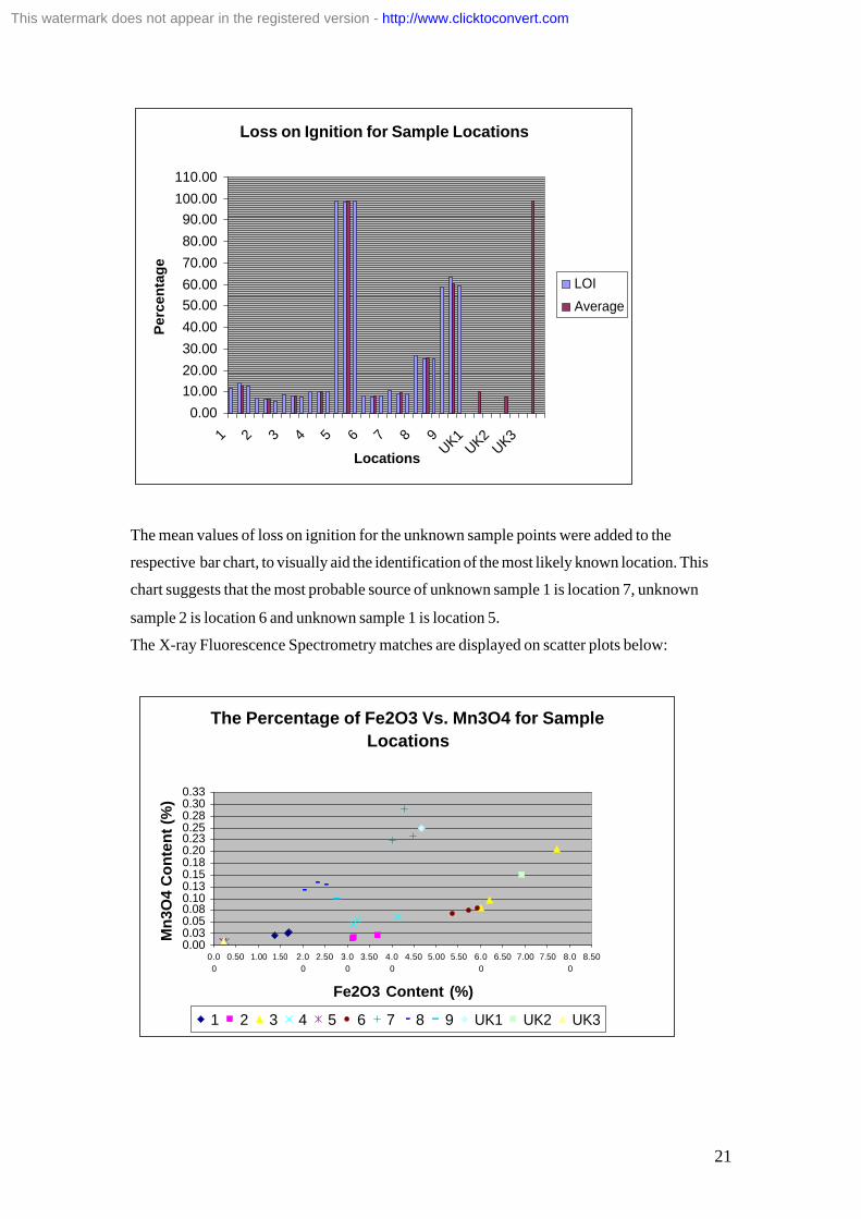
The 3 unknown sample locations were matched to the 9 known locations using Loss on

Ignition, X-ray Fluorescence Spectrometry and Chromatography analysis. The aspects of

these analyses used were taken from data analysis conducted on the 9 sample locations. The

part of X-ray Fluorescence Spectrometry used for the match was elemental composition pairs,

Fe2O3 Vs. Mn3O4, SiO2 Vs. Mn3O4 and K2O Vs. Mn3O4. The part of Chromatography

used to find a match were mean reflectance curves and colour component pairs b* Vs. L* and

C* Vs. L*.

The Average Loss on Ignition values for the unknown sample locations were compared with

those of the known locations on a bar chart below:



21

Loss on Ignition for Sample Locations

0.00

10.00

20.00

30.00

40.00

50.00

60.00

70.00

80.00

90.00

100.00

110.00

1 2 3 4 5 6 7 8 9UK1

UK2

UK3

Locations

Pe

rce

nta

ge

LOI

Average

The mean values of loss on ignition for the unknown sample points were added to the

respective bar chart, to visually aid the identification of the most likely known location. This

chart suggests that the most probable source of unknown sample 1 is location 7, unknown

sample 2 is location 6 and unknown sample 1 is location 5.

The X-ray Fluorescence Spectrometry matches are displayed on scatter plots below:

The Percentage of Fe2O3 Vs. Mn3O4 for Sample

Locations

0.000.030.050.080.100.130.150.180.200.230.250.280.300.33

0.0

0

0.50 1.00 1.50 2.0

0

2.50 3.0

0

3.50 4.0

0

4.50 5.00 5.50 6.0

0

6.50 7.00 7.50 8.0

0

8.50

Fe2O3 Content (%)

Mn

3O

4 C

on

ten

t (%

)

1 2 3 4 5 6 7 8 9 UK1 UK2 UK3



22

The Percentage SiO2 Vs. Mn3O4 for Sample

Locations

0.0000.0130.0250.0380.0500.0630.0750.0880.1000.1130.1250.1380.1500.1630.1750.1880.2000.2130.2250.2380.2500.2630.2750.2880.3000.313

0.00 20.00 40.00 60.00 80.00

SiO2 Content (%)

Mn

3O

4 C

on

ten

t (%

)

1

2

3

4

5

6

7

8

9

UK1

UK2

UK3

The Percentage K2O Vs. Mn3O4 for Sample Locations

0.00

0.02

0.04

0.06

0.08

0.10

0.12

0.14

0.16

0.18

0.20

0.22

0.24

0.26

0.28

0.30

0.32

0.00 0.20 0.40 0.60 0.80 1.00 1.20 1.40 1.60 1.80 2.00 2.20 2.40

K2O Content (%)

Mn

3O

4 C

on

ten

t (%

)

1

2

3

4

5

6

7

8

9

UK1

UK2

UK3



23

The average elemental compositions contents for the unknown locations were added to their

respective scatter plots, to indicate whether there values resided near or within a cluster of

sample points from a known location.

The pairs of elemental compositions Fe2O3 Vs. Mn3O4, SiO2 Vs. Mn3O4, and K2O Vs.

Mn3O4 indicate that the most probable source of unknown sample 1 is location 7, unknown

sample 2 is location 3 and unknown sample 3 is location 5. It is important to note that the pair

of elemental compositions SiO2 Vs. Mn3O4 indicates an uncertainty in the source of sample

2 (i.e. whether location 3 or 8).

The Chromatography matches are displayed below:

The Mean Reflectance Curves for the Sample Locations

0.00

5.00

10.00

15.00

20.00

25.00

30.00

35.00

40.00

400 450 500 550 600 650 700

Wavelength 400-700nm

Pe

rce

nta

ge L

igh

t R

efl

ec

ted

1 2 3 4 5 6 7 8 9 Unknown 1 Unknown 2 Unknown 3

This graph suggests that the most probable source of unknown sample 1 is location 7,

unknown sample 2 is location 6 and unknown sample 3 is location 5. The source of unknown

samples 1 and 3 appear conclusive as there reflectance curves overlay known locations

reflectance curves almost exactly.

The paired colour component matches are displayed on scatter plots below:



24

The Colour Components B* Vs. L* for Sample

Locations

25.0026.0027.0028.0029.0030.0031.0032.0033.0034.0035.0036.0037.0038.0039.0040.0041.0042.0043.0044.0045.0046.0047.0048.0049.0050.0051.0052.0053.0054.0055.0056.0057.0058.0059.00

5.00 7.00 9.00 11.00 13.00 15.00 17.00 19.00 21.00 23.00 25.00

B*

L*

1 2 3 4

5 6 7 8

9 Unknown 1 Unknown 2 Unknown 3

The Colour Components C* Vs. L* for Sample

Locations

25.0026.0027.0028.0029.0030.0031.0032.0033.0034.0035.0036.0037.0038.0039.0040.0041.0042.0043.0044.0045.0046.0047.0048.0049.0050.0051.0052.0053.0054.0055.0056.0057.0058.0059.00

5.00 7.00 9.00 11.00 13.00 15.00 17.00 19.00 21.00 23.00 25.00 27.00

C*

L*

1 2 3 4

5 6 7 8

9 Unknown 1 Unknown 2 Unknown 3

The average colour component values for the unknown locations were added to their

respective scatter plots, to indicate whether there values resided near or within a cluster of

sample points from a known location.

The pairs of colour components B* Vs. L* and C* Vs. L* indicate that the most probable

source of unknown sample 1 is location 7, unknown sample 2 is location 6 and unknown

sample 3 is location 5. There is uncertainty with the indication of the source of unknown



25

sample 2 with respects to C* Vs. L*. If more sample points were taken for locations 6 and 8

this uncertainty may be reduced.

4.42 Probable Vs. Actual

The actual locations of the unknown samples are displayed below:

Location No. Actual Location No.

Unknown 1 7

Unknown 2 Random

Unknown 3 5

The locations established from analysis are displayed below:

Method of

Matching

Location No. Probable Location

No.

Unknown 1 7

Unknown 2 6

Loss on Ignition

Unknown 3 5

Unknown 1 7

Unknown 2 3

Fe2O3 Vs. Mn3O4

Unknown 3 5

Unknown 1 7

Unknown 2 3/ 8

SiO2 Vs. Mn3O4

Unknown 3 5

Unknown 1 7

Unknown 2 3

K2O Vs. Mn3O4

Unknown 3 5

Unknown 1 7

Unknown 2 6

Reflectance Curve

Unknown 3 5

Unknown 1 7

Unknown 2 6

b* Vs. L*

Unknown 3 5

Unknown 1 7

Unknown 2 6/ 8

C* Vs. L*

Unknown 3 5



26

In conclusion, the methods of matching are accurate under this data set. However there is no

method for establishing that a soil does not belong to a sample location. It is important to

stipulate that the matching methods can only be accurate with accordance to the data of

sample locations held. If there are limited sample points of a location this may cause

inaccuracy, but cannot be alleviated unless further samples are conducted. The matching

methods are incapable of producing a specific probability of accuracy, other than ranking the

most probable locations according to matching values or quadratic equations (i.e. reflectance

curve).

The implementation and precision of these matching methods is discussed in the Design/

Implementation section of the report.

5. Project Management

The Initial Schedule and Reviewed Schedule can be seen in Appendix F.

5.1 Initial Schedule

5.11 Performance

The schedule was adequate for the year 2003. It ensured that I became familiar with the user

requirements for the system. This familiarity was sought with three meetings with the

problem owner. Statistical techniques were researched in this period for pre-arranged data.

However it was not possible to investigate statistical methods specific to the data, because the

data had not been collected at this stage. The schedule did not account for later time spent

researching specific statistical methods. Background reading was done before the schedule

announced it, because it was important to understand soil concepts as soon as possible. The

schedule indicated to familiarise with software tools late in the year, which was met without

specific attention, because modules taken incorporated learning to use software that was

relevant (i.e. DB31 – ArcView). The deliverable were not produced due to coursework

commitments, but the write up of these deliverable was not perceived as a big task because all

of the groundwork had been done.

The Christmas break was spent revising for examinations and concentrating on the acquisition

of data. Early February had arrived and the pre-arranged data had been delayed. This resulted

in a re-shuffle in the schedule, as although time could be spent familiarising with software

tools, a time slot for data analysis would have to be made available later in the schedule.



27

Hence secondary requirement capture was brought forward to make a slot available for data

analysis. However this could only be conducted at a high level of abstraction, because

specifics related to data and its analysis were unknown at this stage. Due to the delay of data

acquisition it was sought to seek alternative sources of data. This occupied the majority of

time until early March with no positive feedback received. It was mid-March before the pre-

arranged data was received. This had obvious implications, I was six weeks behind schedule

and not one of the deliverables had been completed.

It was time to review the schedule to make use of the limited time left to complete the

project.

5.12 Major Factor Influencing Performance

· Too reliant on pre-arranged data

· No substitute data organised.

5.2 Schedule Amendments

5.21 Amendments

The review schedule spanned from 23rd

March to 28th

April broken down into three-day time

periods, allowing for one day off a week. It was important to organise the objectives so that

they incorporated the deliverables due to time restrictions. The objectives were broken down

into specific chapters that would be included in the report and allocated time slots for

completion. Time was allocated at the end of the schedule for the review of the report. A

predominant amount of time was allocated to the implementation of the demonstrator. The

majority of the time was allocated at the same time as other tasks to allow further

familiarisation with software, with individual time allocated to concentrate on the

implementation alone.

5.22 Major Factor Influencing Amendments

· Time restrictions.

· Underestimation of implementation.



28

5.23 Indication of Success

· Pre-arranged data has been received and further time has been allocated to

implementation.

· The reviewed schedule is more detailed (i.e. 3-day periods rather than 2-week

periods).

· Software for implementation has been selected, so time is not wasted familiarising

with tools that may not be used.

5.3 Review Schedule Performance

The schedule was interrupted by the underestimation of data analysis, which took eight days

not six days that were allocated. However two days that were allocated to time off were

instead used to finish the data analysis to align the project back on schedule. There were no

other interruptions to schedule; instead it was very accurate up until the project had been

completed. Thus, the schedule provided a positive platform for time management.

6. Requirements Specification

6.1 Requirements Capture Techniques

The User requirements were gathered using SQIRO techniquesxxii

. The five techniques are

Sample Documents, Questionnaires, Interviews, Reading/ Research and Observations.

Sample documents involves the study of forms or tables to interpret the input or output of a

system. Questionnaires are used to establish user requirements from a large population

through the provision of documented structured questions (generate quantative data). Whereas

interviews are interactive and allow an interviewer to guide an interviewee to provide more

specific answers to open-ended questions (qualitative data). Research and reading is used to

gain an overview of the working environment. Observations enable user behaviour to be

interpreted, which is particularly useful for studying usability aspects of a system.

6.2 Techniques Used

Reading/ Research was conducted to gain an overview of the nature of soil. This provided

insight into how soil is sampled and analysed. This was important when tables of data

(Sample Documents) were studied to evaluate the input of the proposed system.



29

Understanding the input was pinnacle to understanding output. It also provided direction for

the data analysis the system might conduct to produce output. The users (Problem Owner and

two Undergraduate Students) were consulted through unstructured interview to capture

exactly what input, processing and output must be provided by the proposed system.

6.3 Overview of Information Collected

The result of requirements capture produced the following functional requirements and non-

functional requirements:

6.31 Functional Requirements

· Provide a method of inputting and modifying Location Data (Soil

regions and soil type).

· Provide a method of inputting and modifying Sample Data

(coordinates, chemical and colour data).

· Provide automatic/ manual assignment of Sample Data to Location

Data according to geography.

· Provide visual representation of soil classification of Sample and

Location Data.

· Provide methods for matching Sample data that has no coordinates to

Location Data.

· Provide a means of generating coordinates for Sample data that does

not have coordinates.

· Provide a means of generating a ranked list for the most probable

Location Data that can be assigned to Sample Data with no coordinates.

· Provide alternative matching methods and the option to use a

combination of matching methods.

6.32 Non- Functional Requirements

· A mean reflectance curve must be calculated for sample data.

· The interface should adhere to H.C.I. guidelines.

· There should be a security policy setup that grants appropriate permissions to

users.



30

· There should be a method implemented to backup the system in both the short

term and long term.

· Location data must use Avery’s Soil Classification

· Validation techniques should be enforced on data, particularly to control the entry

of null values

· The methods of matching should be derived from data analysis

6.33 Use Case Diagram

This diagram (See Appendix G) illustrates how users might interact with the system.

6.4 Requirements List

Requirement Type

Requirement The System shall enable:

Import Soil Region data Import Soil Type data Import Soil Description data

Provide a method of importing Location Data (Soil regions and soil type) Import Location Description data

Input/ Update of coordinate data Input/ Update of Loss on Ignition data Input/ Update of SiO2 Content data Input/ Update of TiO2 Content data Input/ Update of Al2O3 Content data Input/ Update of Fe2O3 Content data Input/ Update of Mn3O4 Content data Input/ Update of MgO Content data Input/ Update of CaO Content data Input/ Update of Na2O Content data Input/ Update of K2O Content data Input/ Update of P2O5 Content data Input/ Update of Cr2O3 Content data Input/ Update of PH in Soil data Input/ Update of Carbonate Content data Input/ Update of reflectance Curve Equation data Input/ Update of L* Component data Input/ Update of a* Component data Input/ Update of b* Component data Input/ Update of C* Component data

Provide a method of inputting and modifying Sample Data (coordinates, chemical and colour data).

Input/ Update of ho Component data

Functional

Provide automatic/ manual assignment of Sample Data to Location Data according to geography

Coordinate Data to be automatically assigned to Soil Region Data



31

Location Data according to geography

Coordinate Data to be manually assigned to Soil Region Data

Spatial representation of Coordinate Data Provide visual representation of soil classification of Sample and Location data

Spatial representation of Soil Region Data

A match to be made with Sample Data with Coordinates and Sample Data without Coordinates

Provide methods for matching Sample data that has no coordinates to Location Data

An assignment of Location Data based on the match of Sample Data with Coordinate data

A coordinate to be generated according to a match on Sample Data with a coordinate.

Provide a means of generating coordinates for Sample data that does not have coordinates

A coordinate from Sample Data that is grouped by Location to be assigned to Sample Data without a Coordinate based on most probable match of Sample Data. Sample Data without a Coordinate to list the closest match of Location Data in ascending order.

Provide a means of generating a ranked list for the most probable Location Data that can be assigned to Sample Data with no coordinates

A weight to be assigned (according to a matching method) to Sample Data grouped by Location that indicates the closeness of match.

A combination of matching methods to be used.

Provide alternative matching methods and the option to use a combination of matching methods A weight representing closeness of

match to be adjusted so that it accounts for a combination of matching methods.

A Reflected Light Percentage to be entered for Wavelengths 400-700nm for Sample Data. A Reflectance Curve Equation to be calculated from Reflected Light Percentage for Wavelengths 400-700nm.

Non -Functional

A mean reflectance curve must be calculated for sample data.

A calculated Reflectance Curve Equation to be assigned to Sample Data.



32

A novice computer user to navigate around and use the system affectively.

The interface should adhere to H.C.I. guidelines.

A novice computer user to quickly learn how to use the system.

Students to add/ modify Sample Data and perform a match. Lecturers to add/ modify Sample Data and Location Data, and also perform a match.

There should be a security policy setup that grants appropriate permissions to users.

An Administrator to have full control. Transactions to be logged and rolled-back if Data has been compromised.

There should be a method implemented to backup the system in both the short term and long term.

Data to be recorded to disk at intervals when the system is not in use for full recovery if the Data has been compromised. Soil Region to be recorded with accordance to Avery’s Soil Classification. Soil Type to be recorded with accordance to Avery’s Soil Classification.

Location data must use Avery’s Soil Classification

Soil Description to be recorded with accordance to Avery’s Soil Classification. Validation of the entry of Reflected Light Percentage to ensure that where Wavelength increases the Reflected Light Percentage increases. Validation of the entry of Chemical Contents to ensure that the sum of values do not exceed 100 and are to 2.d.p’s. Validation of the entry of Colour Components and Loss on Ignition to ensure that values do not exceed 100 and are to 2.d.p’s. Validation of the entry of Soil Region to ensure that its value is unique. Validation of the entry of Sample Data to ensure every record is unique.

Validation techniques should be enforced on data, particularly to control the entry of null values

Validation of other data fields to ensure that they are the correct data type.



33

Sample Data without coordinates to be matched according to the data field Loss on Ignition. Sample Data without coordinates to be matched according to the data fields Fe2O3 Content and Mn3O4 Content. Sample Data without coordinates to be matched according to the data fields SiO2 Content and Mn3O4 Content. Sample Data without coordinates to be matched according to the data fields K2O Content and Mn3O4 Content. Sample Data without coordinates to be matched according to Reflectance Curve Equation. Sample Data without coordinates to be matched according to the data fields b* Component and L* Component.

The methods of matching should be derived from data analysis

Sample Data without coordinates to be matched according to the data fields C* Component and L* Component.

6.5 Prototype Minimum Requirements

The Requirements List was examined by the Problem Owner and agreed that the following

Requirements must be implemented for the prototype:

Requirement Type

Requirement The System shall enable:

Input/ Update of coordinate data Input/ Update of Fe2O3 Content data

Input/ Update of SiO2 Content data

Input/ Update of Mn3O4 Content data

Provide a method of inputting and modifying Sample Data

Input/ Update of K2O Content data

Functional


Coordinate Data to be manually assigned to Soil Region Data



34

Spatial representation of Coordinate Data Provide visual representation of soil classification of Sample and Location data

Spatial representation of Soil Region Data

A match to be made with Sample Data with Coordinates and Sample Data without Coordinates


An assignment of Location Data based on the match of Sample Data with Coordinate data

Provide alternative matching methods and the option to use a combination of matching methods

A combination of matching methods to be used.

A novice computer user to navigate around and use the system affectively.

The interface should adhere to H.C.I. guidelines.

A novice computer user to quickly learn how to use the system.

Sample Data without coordinates to be matched according to the data fields Fe2O3 Content and Mn3O4 Content.

Sample Data without coordinates to be matched according to the data fields SiO2 Content and Mn3O4 Content.

Non -Functional


Sample Data without coordinates to be matched according to the data fields K2O Content and Mn3O4 Content.

6.6 Software The Spatial representation of data led to two main solutions, either the construction of a

Spatial Database or a Geographical Information System. A variety of established software is

available purpose built for constructing a GIS, whereas software is not readily available for

the construction of spatial databases. However, there is a wide range of database product that



35

can be extended to provide spatial functionality. This consideration forced the use of GIS

software.

The GIS software considered was that available within the School of Computing. The choice

available was either ArcView or MapInfo. Both software products provide almost identical

functionality. The decision was therefore base on familiarity of the software. ArcView had

been studied in a Databases Module, so was chosen as the software to implement the

prototype.

7. Design/ Implementation

7.1 Introduction

The design and implementation of the prototype were conducted synchronously, so this

section will describe the implementation and its design considerations.

ArcView uses an object-orientated scripting language called Avenue. Avenue was the

language used to compose all scripts involved in the implementation of the project.

7.2 Data Structure

ArcView represents spatial data using Features, which take the form of a polygon, polyline,

multi-point, point, etc… The Features are held in a Theme. A Theme holds a collection of

Features that may have associated non-spatial attributes that are held in an associated Table

(FTab). A collection of Themes is held in a View.

It was identified from the prototype minimum requirements that the system had hold location

and sample data. The location data would be imported into the system as a theme, including a

feature for Soil Region (as a polygon) and the associated non-spatial attributes: Soil Type (as

a string), Soil Description (as a string) and Location Description (as a string). Constraints on

the length of values permitted for entry into the non-spatial fields could not be imposed, as

they were unknown. The Sample data would be held in a theme that included a feature

representing coordinate data (as a point) and associated non-spatial attributes: Fe2O3 Content

(as a number, length (6), 2dp’s), SiO2 Content (as a number, length (6), 2dp’s), Mn3O4

Content (as a number, length (6), 2dp’s) and K2O Content (as a number, length (6), 2dp’s).



36

A View (‘Location and Sample Data’) was created to hold the two Themes ‘Sample’ and

‘Location’. Although the minimum requirements did not state that Location data had to be

capable of being imported into the system, it was pinnacle to the functionality of the system

that Location data was present and represented in the system. A script (Appendix H) was

developed to generate the Theme and respective table. The Soil Region data was unique so

every record in the FTab could be identified from this A non-spatial attribute Locid was

introduced to also uniquely identify the records, because it was unknown at this stage whether

a spatial attribute would be proficient. A theme was created to hold the Sample data using

graphical features present in ArcView. The Coordinate data was not unique for each sample,

so the attribute Sample ID was introduced to ensure every record in the FTab was unique (a

Location attribute was also introduced to reference the location name).

The coordinates to create the respective polygons and points were retrieved by mapping the

sample points onto Avery’s Soil Map. Then tracing the points and associated soil regions onto

graph paper, where relative X and Y coordinates were gathered. The Themes and associated

FTabs are in Appendix I.

The minimum requirements made it clear that it was important to be able to associate the Soil

Region polygon with the Coordinate data points. ArcView provides a method of creating a

spatial join on ‘Shape’ attributes. A script (Appendix J) was developed to join the features.

This results in the non-spatial attribute data within the Location theme being placed in the

Sample FTab respectively. The format of the Sample FTab is demonstrated in Appendix K.

7.3 Input

The input of the system was concerned with the entry of Sample data in the format of: Shape

(point), Sample id (as a string), (Fe2O3 Content (as a number), SiO2 Content (as a number),

Mn3O4 Content (as a number) and K2O Content (as a number), Location (as a string).

The difficulty lied in developing a method to enable a user to input a specific (x, y) coordinate

into the system to be represented as a Feature (as a point). This was tackled by designing and

implementing a Dialog (Appendix L), which enabled a user to enter an X and a Y coordinate

into separate Text-lines. A Text-line was created for the entry of each non-spatial attribute. A

script (Appendix M) was developed and assigned to a Button on the dialog. The script was

designed to find the appropriate field in the Sample FTab and then create a new record by

assigning the values from the respective Text-lines. This allowed the Text-lines for the X and

Y coordinates to be converted into a point before the Shape attribute in the FTab was set.



37

Dialogs have properties to enable a script to be run when it is opened. A script (Appendix N)

was applied to this open property that selected the appropriate View, then Theme.

7.4 Data Analysis

The minimum requirements indicated that a match between sample data without a coordinate

and sample data within the system needed to be made using the following pairs of attributes:

Fe2O3 Content and Mn3O4 Content, SiO2 Content and Mn3O4 Content, and also K2O

Content and Mn3O4 Content.

A decision was made to match sample data without a coordinate to that in the system to

produce a probable Location, by calculating the Minimum and Maximum values for the

chemical components within the system according to Soil Region. Then to develop a query to

test whether the values from the sample data without a coordinate fit within the maximum and

minimum ranges for the respective chemical component data held on the system to identify a

probable Soil Region.

ArcView does not provide a query language; it provides a windowed Query Builder. This

Query Builder has only very basic query construction methods (i.e. >, <, +, etc…). It does not

provide a method to group data according to an attribute.

ArcView instead enables Summarize FTabs to be constructed. This facility allowed an FTab

to be constructed from the Sample data FTab, grouping by Locid (enabled by the spatial join

aforementioned). Hence merging the Shape attribute (point) into a multipoint and calculating

the Maximum and Minimum values for each chemical component (the average was also

calculated for future development). An example of the Summary Theme and FTab is in

Appendix O.

It was pinnacle that the Summary FTab updated when the Sample data FTab was updated.

Hence so an up to date thorough match could be attained. ArcView provides no instrument to

implement this, so the Summary FTab has to be recreated every-time the Sample FTab is

amended. An important function of the code was to first remove any existing Summary FTab,

then create a new one, as the Match needed to reference a Summary FTab in a fixed position.

The script developed to do this is in Appendix P.



38

7.5 Output

The Summary FTab discussed provided the system values of the match. A Dialog (Appendix

Q) was designed to enable the user to enter chemical component values for sample data

without a coordinate in Text-lines. The Text-lines were assigned Real Number type, so that

values could be used in numerical operations. A script (Appendix R) was applied to the open

property of the Dialog that selected the appropriate View, then Theme and set the Text-line

type. A Checkbox was constructed for each chemical component to enable the user to select

which chemical components they intend to find a match from. A script was designed and

implemented to generate and process a query, then select the corresponding features in the

Summary FTab (thus identifying Locid, which identifies a Soil Region). This script

(Appendix S) was assigned to a Button in the Dialog. The script makes a query list dependant

on whether Checkboxes are true/false values. It finds the selection of the first query result

then either keeps the selection or reduces the selection according to proceeding queries in the

list. Thus producing a selection that satisfies the query list.

7.6 Interface

ArcView provides an interface that is usability focussed. It provides a window that

categorises Views (contains Themes) and Tables. This implies that there is no need to extend

the interface to enable Themes and FTab to be accessed. A user can view an FTab quite easily

by selecting a Theme inside a View and selecting the respective drop down menu at the top of

the screen. It is further straightforward to select a record in the FTab and delete the Feature

and associated non-spatial attributes. It is possible to modify non-spatial data this way, but

impossible to modify the Shape attribute. For this reason that is why the Dialog was

developed for adding Sample data.

A Dialog (Appendix T) was created to provide the user with easy access to the Add Sample

Dialog, Match Dialog, and also to execute the script to recreate the Summary FTab. A Button

was created and scripts assigned to summon the Add Sample and Match Dialogs. The script

to create the Summary table was assigned to a Button. A script was created to display this

Dialog and assigned to a Button on the Project toolbar for ease of access. The scripts assigned

to the respective Buttons are displayed in Appendix U.



39

8. Evaluation

8.1 Testing and Performance

8.11 Introduction

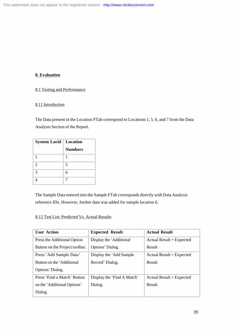
The Data present in the Location FTab correspond to Locations 1, 5, 6, and 7 from the Data

Analysis Section of the Report.

System Locid Location

Numbers

1 1

2 5

3 6

4 7

The Sample Data entered into the Sample FTab corresponds directly with Data Analysis

reference IDs. However, further data was added for sample location 6.

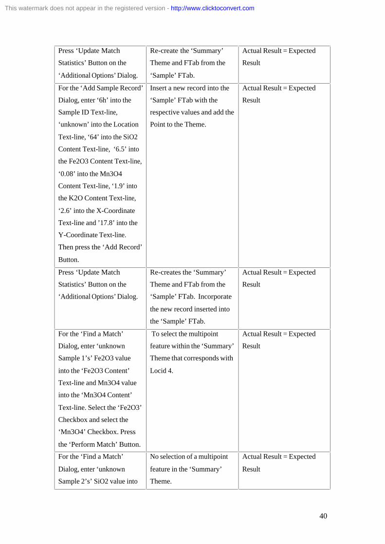
8.12 Test List: Predicted Vs. Actual Results

User Action Expected Result Actual Result

Press the Additional Option

Button on the Project toolbar.

Display the ‘Additional

Options’ Dialog.

Actual Result = Expected

Result

Press ‘Add Sample Data’

Button on the ‘Additional

Options’ Dialog.

Display the ‘Add Sample

Record’ Dialog.


Result

Press ‘Find a Match’ Button

on the ‘Additional Options’

Dialog.

Display the ‘Find A Match’

Dialog.


Result



40

Press ‘Update Match

Statistics’ Button on the

‘Additional Options’ Dialog.

Re-create the ‘Summary’

Theme and FTab from the

‘Sample’ FTab.


Result

For the ‘Add Sample Record’

Dialog, enter ‘6h’ into the

Sample ID Text-line,

‘unknown’ into the Location

Text-line, ‘64’ into the SiO2

Content Text-line, ‘6.5’ into

the Fe2O3 Content Text-line,

‘0.08’ into the Mn3O4

Content Text-line, ‘1.9’ into

the K2O Content Text-line,

‘2.6’ into the X-Coordinate

Text-line and ’17.8’ into the

Y-Coordinate Text-line.

Then press the ‘Add Record’

Button.

Insert a new record into the

‘Sample’ FTab with the

respective values and add the

Point to the Theme.


Result

Press ‘Update Match

Statistics’ Button on the

‘Additional Options’ Dialog.

Re-creates the ‘Summary’

Theme and FTab from the

‘Sample’ FTab. Incorporate

the new record inserted into

the ‘Sample’ FTab.


Result

For the ‘Find a Match’

Dialog, enter ‘unknown

Sample 1’s’ Fe2O3 value

into the ‘Fe2O3 Content’

Text-line and Mn3O4 value

into the ‘Mn3O4 Content’

Text-line. Select the ‘Fe2O3’

Checkbox and select the

‘Mn3O4’ Checkbox. Press

the ‘Perform Match’ Button.

To select the multipoint

feature within the ‘Summary’

Theme that corresponds with

Locid 4.


Result



Sample 2’s’ SiO2 value into

the ‘SiO2 Content’ Text-line

and Mn3O4 value into the

‘Mn3O4 Content’ Text-line.

Select the ‘SiO2’ Checkbox

and select the ‘Mn3O4’

No selection of a multipoint

feature in the ‘Summary’

Theme.


Result



41

the ‘SiO2 Content’ Text-line



Select the ‘SiO2’ Checkbox


Checkbox. Press the

‘Perform Match’ Button.



Sample 3’s’ K2O value into

the ‘K2O Content’ Text-line



Select the ‘K2O’ Checkbox


Checkbox. Press the

‘Perform Match’ Button.

To select the multipoint

feature within the ‘Summary’

Theme that corresponds with

Locid 2.


Result

8.13 Functional Performance

The results from the test plan indicate that the functional implementation of the system was a

success. However, it does not examine whether functional implementation met functional

minimum requirements for the prototype. The following table identifies the prototype

minimum functional requirements and discusses the degree to which the system satisfies the

functionalities.

Functional

Requirement

Prototype Provision

Provide a method of inputting and modifying Sample Data

A Dialog was provided to aid the input of Sample data, in particular

the input of point data. Further implementation was not made to aid

modification and deletion of Sample data. ArcView provides options

that facilitate this functionality. However, neither ArcView nor the

system provides a competent method for editing point data. For

example, if the point data required editing the feature and record

would have to be removed and an up to date record inserted.



42


Creating a spatial join between the shape attributes in the Sample

FTab and Location FTab fulfilled this requirement. This provided an

automatic method of assigning Sample data to Location data. The

nature of a spatial join means that if either data set is updated, so is

the assignment.

Provide visual

representation of soil

classification of

Sample and Location

data

Representing Location data’s Soil region and Sample data’s

Coordinate data using Features provided this functionality.


This was provided through the constructing a Summary FTab that was

queried through a Dialog. This used very basic statistics in the form of

ranges, identifying maximum and minimum values for each chemical

component grouped by location for system data, then finding the

range that the sample data without a coordinate fell into. The accuracy

of a statistical match was highly dependant on the number of sample

point within in a location. Also it did not account for variation of soil

properties within soil region. However the data provided did not allow

this approach to be developed. Hence, although the statistics were

basic, data analysis demonstrated that the variables used were very

affective discriminators. The system provided extra functionality as it

identified graphically the most appropriate match.

Provide alternative

matching methods

and the option to use

a combination of

matching methods

The querying technique for a match was formulated to adjust

according to Checkboxes attached to the respective Dialog. Each

Checkbox represented one of four chemical compositions that could

be included within the range query or otherwise. The system did not

provide a matching method for neither colour analysis nor loss on

ignition that had been identified in data analysis as good

discriminators.

8.14 Non-functional Performance

Non-functional Requirement

Prototype Provision

The interface should adhere to H.C.I. guidelines

xxiii.

ArcView restricted HCI development as buttons added to toolbar take a standard form. Dialogs are restricted to a standard font, colour, etc.... However ArcView does provide a consistent user interface with the provision of a window to control access to documents (Views, Tables, Scripts, etc…). Upon selection the toolbar is modified according to the document type to aid user interaction. Also the standard Dialogs do adhere to a competent degree of usability. ArcView provides a good degree of learnability due to a consistent interface and well placed features, and with additional Dialogs implemented for



43

to documents (Views, Tables, Scripts, etc…). Upon selection the toolbar is modified according to the document type to aid user interaction. Also the standard Dialogs do adhere to a competent degree of usability. ArcView provides a good degree of learnability due to a consistent interface and well placed features, and with additional Dialogs implemented for Additional Options, Adding Sample data and Matching, it is clear that adequate attempts have been made to adhere to HCI guidelines.


The system provides a match based on the chemical components that were identified within data analysis as having high discriminatory power.

8.15 User Response

A subject was exposed to the following Training Schedule and a User Manual (Appendix V),

then interviewed and observed to gather their response to the system.

8.151 Training Schedule (15 minutes)

· Introduction to ArcView Document Control Window.

· Accessing a Theme through a View and selecting an FTab

· Selecting a Feature in a Theme and FTab

· Deleting a Record of an FTab

· Navigation of Additional Options Dialog

· Introduction to Add Sample and Match Dialogs

· Implication of adding sample data and match results

· Introduction to legend editor

8.152 Interview and Observation of User

The subject had no difficulties interacting with the system. The user navigated around the

system with no problem adding and deleting sample data. The user conducted a match with

relative ease. The user noted that the process for deleting records from the Sample VTab was

confusing and time consuming, and a Dialog to find and delete a record would be more

suited. The subject suggested implementing the Theme so that they automatically use

different coloured features for each item, rather than the user having to set this up them-



44

selves. The user observed that when the match statistics are updated (i.e. the Summary FTab),

and then the table for the Theme is viewed, it creates a new FTab without deleting the

previous one. This leaves one Theme but two tables. The user stated that this might cause

confusion and suggested implementing the system, so that it is automatically removes one

table before allowing another to be created.

8.2 Recommendations The system’s major purpose was to match a soil sample with a database holding site

information to determine the most probable site the sample came from. The match can only

be as good as the statistics implemented. Strenuous data analysis was conducted, however the

findings were not fully implemented. It would be recommended for future development to

concentrate on the implementation of a match according to a Reflectance curve. This showed

a high degree of distinguish-ability in data analysis. The equation could be modelled using

polynomial representation, which are well suited to computers in terms of speed and

accuracy. This introduction of complex statistics gives rise to recommending the investigation

and perhaps integration of MatLab. This software was purpose built to perform statistical

operations.

It is also recommended with respect to statistical matching that multi-variant analysis be

further investigated. This is because the behaviour of paired soil measurements were

considered, however the behaviour of three or more attributes may lead to a more

comprehensive match.

A larger volume of sample data would give rise to other forms of analysis, such as data

mining. Data mining enables the classification of data into various grouping according to

rules that are developed. This implies that sample data could be grouped by location and used

to formulate a statistical match. The rules are used to produce a decision tree (e.g. if X go

down the left branch, if Y go down the right branch, then given that X is it Xa or Xb, etc…).

It is recommended that this be investigated for full implementation, as the rules could be

coded into an Avenue script to produce a match.

It was apparent through the implementation of the prototype that ArcView’s options for

extending the interface are very restrictive. It is recommended that a generic scripting

language (i.e. Visual Basics) be used to produce an interface that adheres to HCI guidelines.

User response to the prototype indicated that methods for deleting and modifying records

were both laborious and time consuming. It is recommended that the system include an

interface for this procedure enabling a user to search, find and delete or modify a record. Also

methods of modifying spatial data need to be implemented, rather that the current process of

deleting and inserted a new record. It was also noted that the recreation of the Summary



45

theme resulted in more that one associated tables. Hence it is recommended to implement a

method to resolve this system flaw. The final observation by the user was concerning the

manual customisation of the Features through the legend editor. The user claimed it was both

confusing and not straightforward. Thus, it is recommended that this procedure be automated

in the final system.

The usefulness of user feedback support the recommendation of building further prototypes

incorporating more system functionality, rather than attempting to build the full system

straight away.

ArcView does not provide a query language, which may cause difficulties if more complex

queries require implementation. This concern drives the recommendation of an investigation

into the implementation of the system using MapInfo. This is another GIS software product

that supports a common query language SQL. The decision from this investigation is pinnacle

in further prototype developments. Due to this consideration it is recommended that Location

data that is purchased should be of MapInfo file type, as both software products support this

and thus could import it into the system.



I

Appendix A The project was accepted without fully understanding the degree of reliance upon

other for the provision of data. I was informed that I would receive data before the

Christmas break, which I required to perform data analysis. Data analysis was the

backbone to the entire project. This data was not received in due time, because those

gathering it ran over their schedule. This caused huge delays and disruption to my

project schedule, which caused a complete redesign of my schedule. I certainly would

not part take in another project that holds such a reliance on others. In hindsight I

would have prepared alternative data sources and would recommend that those who

partake in similar project do just that.

The software to be used for implementation was selected without fully evaluating its

capabilities. This caused problems when implementing a match. ArcView does not

have a supporting query language. Instead, it has to be integrated with a database, or

object-orientated scripts have to be created to perform a query. This resulted in the

implementation of Avenue scripts, as the scale of implementation did not warrant the

design and integration of a database. I had limited experience of object-orientated

programming and thus underestimated the steep learning curve to using Avenue

scripting language. Hence in hindsight I would have elected to use software that had a

supporting query language. I have learnt that selecting appropriate tools for

implementation is very important, and I would recommend that future students do not

take this decision likely.

The mishaps involving data acquisition led to the revaluation of a project schedule.

This reviewed schedule was more detailed in terms of the decomposition of tasks and

duration in which tasks should be completed. This provided an important framework

for time management and completing the project on time. The schedule brought the

project back on schedule, which emphasised it importance. A realistic detailed

schedule is pinnacle to project completion and I would emphasise to anyone about to

conduct a project its importance and potential impact.



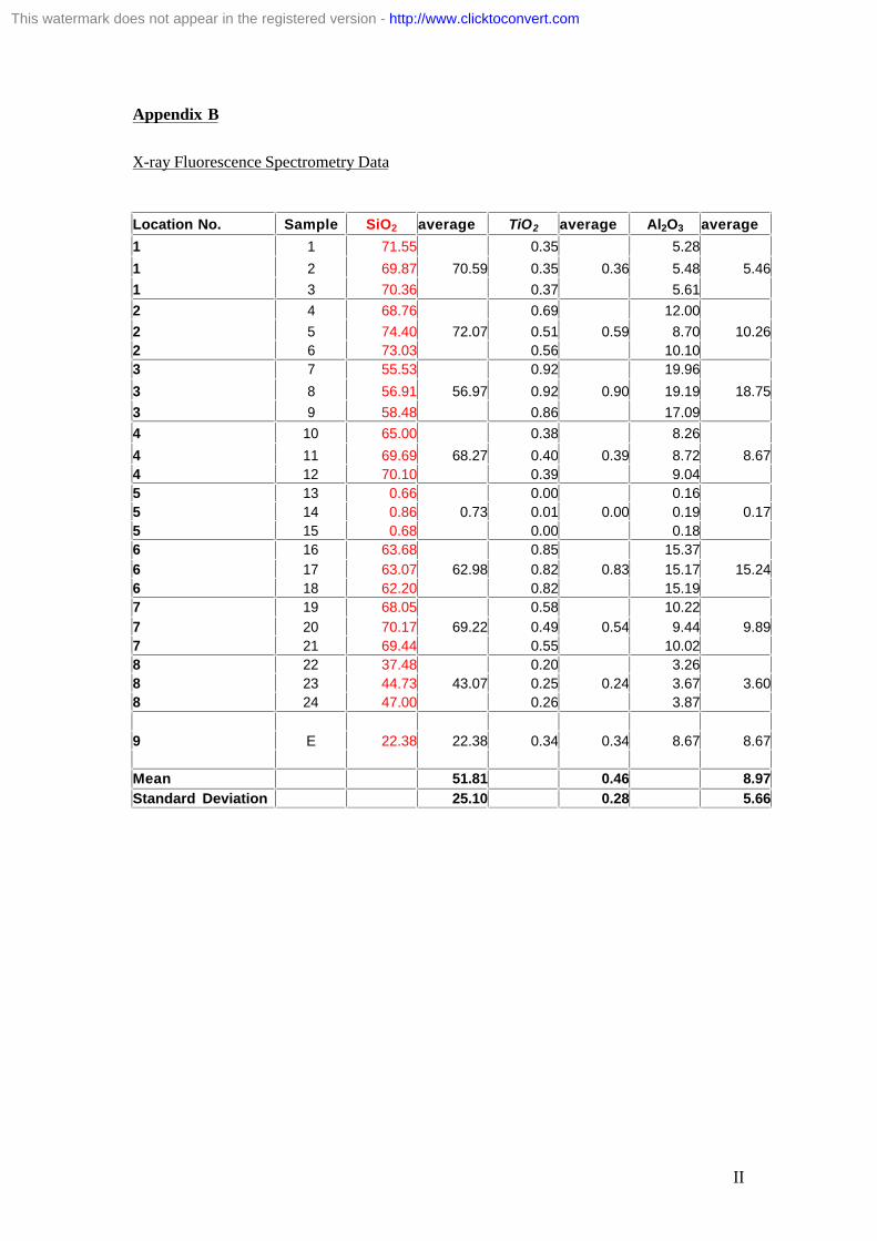
II

Appendix B

X-ray Fluorescence Spectrometry Data Location No. Sample SiO2 average TiO2 average Al2O3 average

1 1 71.55 0.35 5.28

1 2 69.87 70.59 0.35 0.36 5.48 5.46

1 3 70.36 0.37 5.61

2 4 68.76 0.69 12.00

2 5 74.40 72.07 0.51 0.59 8.70 10.26

2 6 73.03 0.56 10.10

3 7 55.53 0.92 19.96

3 8 56.91 56.97 0.92 0.90 19.19 18.75

3 9 58.48 0.86 17.09

4 10 65.00 0.38 8.26

4 11 69.69 68.27 0.40 0.39 8.72 8.67

4 12 70.10 0.39 9.04

5 13 0.66 0.00 0.16

5 14 0.86 0.73 0.01 0.00 0.19 0.17

5 15 0.68 0.00 0.18

6 16 63.68 0.85 15.37

6 17 63.07 62.98 0.82 0.83 15.17 15.24

6 18 62.20 0.82 15.19

7 19 68.05 0.58 10.22

7 20 70.17 69.22 0.49 0.54 9.44 9.89

7 21 69.44 0.55 10.02

8 22 37.48 0.20 3.26

8 23 44.73 43.07 0.25 0.24 3.67 3.60

8 24 47.00 0.26 3.87

9 E 22.38 22.38 0.34 0.34 8.67 8.67

Mean 51.81 0.46 8.97

Standard Deviation 25.10 0.28 5.66



III

Fe2O3 average Mn3O4 average MgO average CaO average Na2O average

1.38 0.02 0.30 1.42 0.40

1.65 1.57 0.03 0.03 0.27 0.28 0.99 1.07 0.37 0.39

1.68 0.03 0.26 0.81 0.39

3.70 0.02 0.82 0.06 0.73

3.13 3.33 0.01 0.02 0.49 0.65 0.05 0.06 0.89 0.79

3.15 0.02 0.63 0.06 0.74

6.19 0.10 0.94 0.02 0.36

6.02 6.64 0.08 0.13 0.93 0.89 0.01 0.01 0.33 0.36

7.71 0.21 0.80 0.01 0.39

3.14 0.05 0.35 0.09 0.84

4.12 3.50 0.06 0.05 0.38 0.37 0.10 0.09 0.91 0.88

3.24 0.05 0.37 0.10 0.91

0.27 0.01 0.15 0.04 0.12

0.21 0.23 0.01 0.01 0.15 0.15 0.06 0.05 0.11 0.09

0.23 0.01 0.15 0.05 0.02

5.93 0.08 1.14 0.08 0.91

5.74 5.68 0.07 0.07 1.11 1.11 0.09 0.08 1.12 1.03

5.37 0.07 1.07 0.08 1.05

4.29 0.29 0.39 0.26 0.56

4.00 4.26 0.22 0.25 0.35 0.37 0.23 0.25 0.59 0.66

4.48 0.23 0.36 0.25 0.85

2.00 0.12 9.73 15.08 0.47

2.29 2.26 0.13 0.13 8.41 8.51 13.59 13.32 0.28 0.35

2.49 0.13 7.39 11.30 0.30

2.77 2.77 0.10 0.10 0.47 0.47 0.12 0.12 0.24 0.24

3.36 0.09 1.42 1.67 0.53

1.98 0.08 2.68 4.38 0.32



IV

K2O average P2O5 average Cr2O3 average

1.25 0.27 0.02

1.40 1.38 0.34 0.32 0.03 0.02

1.49 0.36 0.03

1.72 0.09 0.01

1.19 1.45 0.07 0.08 0.01 0.01

1.44 0.08 0.01

2.28 0.07 0.02

2.24 2.22 0.07 0.07 0.02 0.02

2.15 0.07 0.02

1.65 0.22 0.01

1.69 1.71 0.24 0.23 0.01 0.01

1.79 0.23 0.01

0.01 0.04 0.00

0.01 0.01 0.04 0.04 0.00 0.00

0.01 0.05 0.00

1.72 0.11 0.02

1.70 1.79 0.11 0.11 0.02 0.02

1.94 0.10 0.01

0.99 0.10 0.01

0.94 1.01 0.09 0.10 0.01 0.01

1.09 0.10 0.01

0.58 0.05 0.00

0.69 0.65 0.06 0.06 0.01 0.00

0.70 0.07 0.01

1.31 1.31 0.05 0.05 0.08 0.08

1.28 0.12 0.02

0.66 0.10 0.02



V

Loss on Ignition, Soil PH in Water and Soil Carbonate Data

sample pH average CO3 average LOI average

1 6.56 0.0863 11.68

1 6.58 6.56 0.0740 0.0653 14.08 12.79

1 6.54 0.0356 12.61

2 4.49 0.0857 6.87

2 4.42 4.43 0.0709 0.0696 6.38 6.36

2 4.39 0.0523 5.83

3 4.31 0.0521 8.61

3 4.33 4.33 0.0501 0.0509 8.14 8.18

3 4.35 0.0505 7.79

4 4.80 0.0873 10.16

4 4.69 4.71 0.0850 0.0761 10.22 10.24

4 4.65 0.0559 10.34

5 4.53 0.0053 99.02

5 4.16 4.21 0.0191 0.0109 98.39 98.75

5 3.93 0.0082 98.85

6 4.61 0.0251 8.01

6 4.47 4.52 0.0285 0.0223 7.73 7.90

6 4.47 0.0132 7.96

7 5.68 0.0344 10.40

7 5.73 5.70 0.0201 0.0264 9.16 9.57

7 5.69 0.0246 9.16

8 7.69 0.2526 26.79

8 7.89 7.82 0.2127 0.2182 25.58 25.88

8 7.89 0.1894 25.26

9 4.55 0.0314 58.57



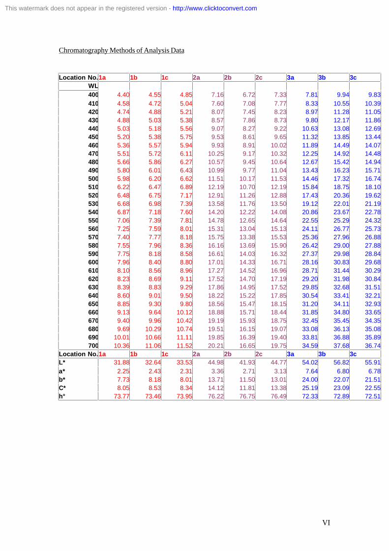
VI

Chromatography Methods of Analysis Data Location No. 1a 1b 1c 2a 2b 2c 3a 3b 3c

WL

400 4.40 4.55 4.85 7.16 6.72 7.33 7.81 9.94 9.83

410 4.58 4.72 5.04 7.60 7.08 7.77 8.33 10.55 10.39

420 4.74 4.88 5.21 8.07 7.45 8.23 8.97 11.28 11.05

430 4.88 5.03 5.38 8.57 7.86 8.73 9.80 12.17 11.86

440 5.03 5.18 5.56 9.07 8.27 9.22 10.63 13.08 12.69

450 5.20 5.38 5.75 9.53 8.61 9.65 11.32 13.85 13.44

460 5.36 5.57 5.94 9.93 8.91 10.02 11.89 14.49 14.07

470 5.51 5.72 6.11 10.25 9.17 10.32 12.25 14.92 14.48

480 5.66 5.86 6.27 10.57 9.45 10.64 12.67 15.42 14.94

490 5.80 6.01 6.43 10.99 9.77 11.04 13.43 16.23 15.71

500 5.98 6.20 6.62 11.51 10.17 11.53 14.46 17.32 16.74

510 6.22 6.47 6.89 12.19 10.70 12.19 15.84 18.75 18.10

520 6.48 6.75 7.17 12.91 11.26 12.88 17.43 20.36 19.62

530 6.68 6.98 7.39 13.58 11.76 13.50 19.12 22.01 21.19

540 6.87 7.18 7.60 14.20 12.22 14.08 20.86 23.67 22.78

550 7.06 7.39 7.81 14.78 12.65 14.64 22.55 25.29 24.32

560 7.25 7.59 8.01 15.31 13.04 15.13 24.11 26.77 25.73

570 7.40 7.77 8.18 15.75 13.38 15.53 25.36 27.96 26.88

580 7.55 7.96 8.36 16.16 13.69 15.90 26.42 29.00 27.88

590 7.75 8.18 8.58 16.61 14.03 16.32 27.37 29.98 28.84

600 7.96 8.40 8.80 17.01 14.33 16.71 28.16 30.83 29.68

610 8.10 8.56 8.96 17.27 14.52 16.96 28.71 31.44 30.29

620 8.23 8.69 9.11 17.52 14.70 17.19 29.20 31.98 30.84

630 8.39 8.83 9.29 17.86 14.95 17.52 29.85 32.68 31.51

640 8.60 9.01 9.50 18.22 15.22 17.85 30.54 33.41 32.21

650 8.85 9.30 9.80 18.56 15.47 18.15 31.20 34.11 32.93

660 9.13 9.64 10.12 18.88 15.71 18.44 31.85 34.80 33.65

670 9.40 9.96 10.42 19.19 15.93 18.75 32.45 35.45 34.35

680 9.69 10.29 10.74 19.51 16.15 19.07 33.08 36.13 35.08

690 10.01 10.66 11.11 19.85 16.39 19.40 33.81 36.88 35.89

700 10.36 11.06 11.52 20.21 16.65 19.75 34.59 37.68 36.74

Location No. 1a 1b 1c 2a 2b 2c 3a 3b 3c

L* 31.88 32.64 33.53 44.98 41.93 44.77 54.02 56.82 55.91

a* 2.25 2.43 2.31 3.36 2.71 3.13 7.64 6.80 6.78

b* 7.73 8.18 8.01 13.71 11.50 13.01 24.00 22.07 21.51

C* 8.05 8.53 8.34 14.12 11.81 13.38 25.19 23.09 22.55

h° 73.77 73.46 73.95 76.22 76.75 76.49 72.33 72.89 72.51



VII

4a 4b 4c 5a 5b 5c 6a 6b 6c

6.11 5.94 5.73 3.09 2.81 2.99 7.69 7.22 7.63

6.44 6.26 6.05 3.17 2.88 3.07 8.16 7.65 8.07

6.78 6.58 6.37 3.25 2.95 3.15 8.69 8.14 8.58

7.14 6.92 6.72 3.32 3.01 3.22 9.33 8.74 9.18

7.50 7.25 7.06 3.41 3.08 3.3 9.97 9.34 9.8

7.85 7.57 7.39 3.53 3.2 3.38 10.5 9.84 10.36

8.17 7.86 7.71 3.66 3.32 3.49 10.97 10.27 10.84

8.42 8.11 7.97 3.78 3.43 3.61 11.31 10.6 11.17

8.68 8.37 8.22 3.89 3.53 3.73 11.69 10.96 11.53

8.98 8.65 8.52 4 3.63 3.84 12.24 11.47 12.05

9.37 9.00 8.88 4.15 3.76 3.97 12.94 12.13 12.72

9.88 9.47 9.37 4.36 3.97 4.18 13.85 13.01 13.63

10.42 9.96 9.89 4.59 4.19 4.38 14.83 13.95 14.59

10.91 10.40 10.35 4.77 4.35 4.54 15.77 14.85 15.5

11.38 10.82 10.78 4.96 4.51 4.7 16.67 15.71 16.37

11.81 11.21 11.20 5.19 4.72 4.9 17.52 16.52 17.2

12.20 11.57 11.59 5.42 4.94 5.11 18.29 17.24 17.95

12.54 11.89 11.94 5.61 5.11 5.3 18.87 17.81 18.53

12.87 12.19 12.28 5.83 5.32 5.53 19.4 18.33 19.06

13.23 12.53 12.64 6.19 5.66 5.87 19.98 18.9 19.65

13.56 12.83 12.98 6.58 6.03 6.25 20.53 19.42 20.2

13.79 13.06 13.23 6.91 6.33 6.55 20.91 19.78 20.59

14.00 13.26 13.45 7.24 6.65 6.87 21.27 20.14 20.95

14.22 13.52 13.70 7.68 7.05 7.31 21.78 20.64 21.38

14.47 13.81 13.99 8.16 7.5 7.79 22.3 21.16 21.83

14.82 14.13 14.36 8.67 7.99 8.24 22.74 21.6 22.33

15.18 14.44 14.74 9.22 8.52 8.71 23.17 22 22.83

15.49 14.71 15.04 9.8 9.06 9.21 23.62 22.39 23.33

15.80 14.98 15.33 10.42 9.64 9.75 24.08 22.79 23.81

16.14 15.29 15.64 11.08 10.23 10.35 24.53 23.19 24.26

16.49 15.63 15.97 11.77 10.86 11.01 24.98 23.61 24.69

4a 4b 4c 5a 5b 5c 6a 6b 6c

40.65 39.72 39.73 27.75 26.43 27 48.44 47.2 48.08

3.07 2.96 3.26 5.38 5.34 5.3 4.43 4.49 4.43

11.92 11.32 11.99 9.52 9.38 9.1 16.7 16.57 16.52

12.31 11.70 12.43 10.94 10.8 10.54 17.28 17.17 17.1

75.54 75.33 74.78 60.54 60.33 59.77 75.13 74.85 74.97



VIII

7a 7b 7c 8a 8b 8c 9a 9b 9c

6.64 6.59 6.82 8.42 9.77 8.21 6.49 6.61 6.38

7.04 6.99 7.23 8.95 10.36 8.71 6.72 6.83 6.59

7.5 7.45 7.7 9.56 11.04 9.29 6.97 7.06 6.81

8.04 8 8.26 10.29 11.84 9.98 7.23 7.32 7.03

8.59 8.56 8.83 11.04 12.65 10.68 7.49 7.57 7.26

9.02 9.07 9.37 11.73 13.36 11.3 7.71 7.8 7.49

9.41 9.51 9.84 12.35 13.99 11.86 7.91 7.99 7.69

9.75 9.85 10.18 12.82 14.5 12.32 8.07 8.15 7.82

10.13 10.21 10.54 13.31 15.02 12.8 8.22 8.29 7.95

10.63 10.72 11.06 13.96 15.7 13.41 8.4 8.47 8.12

11.24 11.36 11.71 14.75 16.53 14.16 8.63 8.69 8.33

12.02 12.19 12.56 15.74 17.57 15.09 8.93 9.01 8.64

12.85 13.08 13.46 16.8 18.68 16.09 9.24 9.33 8.94

13.63 13.91 14.29 17.79 19.72 17.04 9.48 9.56 9.17

14.37 14.71 15.1 18.81 20.77 18.01 9.68 9.76 9.36

15.1 15.49 15.87 19.89 21.86 19.03 9.87 9.95 9.54

15.76 16.19 16.56 20.95 22.92 20.01 10.03 10.11 9.68

16.3 16.73 17.12 21.87 23.82 20.87 10.13 10.21 9.76

16.8 17.25 17.64 22.73 24.65 21.67 10.22 10.31 9.84

17.37 17.84 18.24 23.59 25.48 22.45 10.37 10.46 9.99

17.9 18.41 18.8 24.33 26.21 23.12 10.53 10.61 10.13

18.26 18.81 19.21 24.82 26.67 23.57 10.61 10.7 10.23

18.62 19.2 19.6 25.23 27.07 23.95 10.67 10.77 10.3

19.2 19.72 20.08 25.69 27.59 24.44 10.76 10.85 10.38

19.79 20.25 20.59 26.18 28.13 24.95 10.86 10.95 10.47

20.21 20.74 21.14 26.74 28.67 25.47 10.97 11.1 10.59

20.59 21.22 21.68 27.31 29.2 25.99 11.09 11.25 10.73

20.98 21.72 22.2 27.86 29.7 26.48 11.22 11.38 10.86

21.37 22.21 22.68 28.38 30.18 26.97 11.34 11.48 10.98

21.78 22.66 23.13 28.86 30.64 27.46 11.43 11.56 11.07

22.2 23.08 23.53 29.31 31.08 27.94 11.52 11.62 11.15

7a 7b 7c 8a 8b 8c 9a 9b 9c

45.45 45.93 46.44 51.57 53.66 50.55 37.31 37.46 36.69

4.52 4.68 4.57 5.59 5.1 5.37 0.93 0.97 0.9

16.12 16.81 16.71 18.48 17.76 17.9 6.76 6.72 6.53

16.74 17.45 17.32 19.3 18.48 18.68 6.83 6.79 6.59

74.33 74.43 74.71 73.17 73.97 73.31 82.19 81.82 82.11



IX

Appendix C

The Percentage SiO2 Composition for Sample

Locations

0.00

5.0010.00

15.0020.00

25.0030.00

35.0040.00

45.00

50.0055.00

60.0065.00

70.0075.00

80.00

1 1 1 2 2 2 3 3 3 4 4 4 5 5 5 6 6 6 7 7 7 8 8 8 9

Locations

Pe

rce

nta

ge

SiO2

average

The Percentage TiO2 Composition for Sample

Locations

0.00

0.10

0.20

0.30

0.40

0.50

0.60

0.70

0.80

0.90

1.00

1 1 1 2 2 2 3 3 3 4 4 4 5 5 5 6 6 6 7 7 7 8 8 8 9

Locations

Pe

rce

nta

ge

TiO2

average



X

The Percentage Al2O3 Composition for Sample

Locations

0.00

2.50

5.00

7.50

10.00

12.50

15.00

17.50

20.00

22.50

1 1 1 2 2 2 3 3 3 4 4 4 5 5 5 6 6 6 7 7 7 8 8 8 9

Locations

Pe

rce

nta

ge

Al2O3

average

The Percentage Fe2O3 Composition for Sample

Locations

0.000.501.001.502.002.503.003.504.004.505.005.506.006.507.007.508.008.50

1 1 1 2 2 2 3 3 3 4 4 4 5 5 5 6 6 6 7 7 7 8 8 8 9

Locations

Pe

rce

nta

ge

Fe2O3

average



XI

The Percentage Mn3O4 Composition for Sample

Locations

0.00

0.03

0.05

0.08

0.10

0.13

0.15

0.18

0.20

0.23

0.25

0.28

0.30

0.33

1 1 1 2 2 2 3 3 3 4 4 4 5 5 5 6 6 6 7 7 7 8 8 8 9

Locations

Pe

rcen

tag

e

Mn3O4

average

The Percentage MgO Composition for Sample

Locations

0.00

1.00

2.00

3.00

4.00

5.00

6.00

7.00

8.00

9.00

10.00

11.00

1 1 1 2 2 2 3 3 3 4 4 4 5 5 5 6 6 6 7 7 7 8 8 8 9

Locations

Pe

rce

nta

ge

MgO

average



XII

The Percentage CaO Composition for Sample

Locations

0.00

1.00

2.00

3.00

4.00

5.00

6.00

7.00

8.00

9.00

10.00

11.00

12.00

13.00

14.00

15.00

16.00

1 1 1 2 2 2 3 3 3 4 4 4 5 5 5 6 6 6 7 7 7 8 8 8 9

Locations

Pe

rcen

tag

e

CaO

average

The Percentage Na2O Composition for Sample

Locations

0.00

0.10

0.20

0.30

0.40

0.50

0.60

0.70

0.80

0.90

1.00

1.10

1.20

1 1 1 2 2 2 3 3 3 4 4 4 5 5 5 6 6 6 7 7 7 8 8 8 9

Locations

Pe

rcen

tag

e

Na2O

average



XIII

The Percentage K2O Composition for Sample

Locations

0.00

0.25

0.50

0.75

1.00

1.25

1.50

1.75

2.00

2.25

2.50

1 1 1 2 2 2 3 3 3 4 4 4 5 5 5 6 6 6 7 7 7 8 8 8 9

Locations

Pe

rcen

tag

e

K2O

average

The Percentage P2O5 Composition for Sample

Locations

0.000

0.025

0.050

0.075

0.100

0.125

0.150

0.175

0.200

0.225

0.250

0.275

0.300

0.325

0.350

0.375

0.400

1 1 1 2 2 2 3 3 3 4 4 4 5 5 5 6 6 6 7 7 7 8 8 8 9

Locations

Pe

rcen

tag

e

P2O5

average



XIV

The Percentage Cr2O3 Composition for Sample

Locations

0.000

0.005

0.010

0.015

0.020

0.025

0.030

0.035

0.040

0.045

0.050

0.055

0.060

0.065

0.070

0.075

0.080

1 1 1 2 2 2 3 3 3 4 4 4 5 5 5 6 6 6 7 7 7 8 8 8 9

Locations

Pe

rcen

tag

e

Cr2O3

average



XV

Appendix D

The Percentage of SiO2 Vs. Fe2O3 for Sample

Locations

0.001.002.003.004.005.006.007.008.009.00

0.00 10.00 20.00 30.00 40.00 50.00 60.00 70.00 80.00

SiO2 Content (%)

Fe2

O3 C

on

ten

t (%

) 1

2

3

4

5

6

7

8

9

The Percentage SiO2 Vs. Mn3O4 for Sample

Locations

0.0000.0130.0250.0380.0500.0630.0750.0880.1000.1130.1250.1380.1500.1630.1750.1880.2000.2130.2250.2380.2500.2630.2750.2880.3000.313

0.00 20.00 40.00 60.00 80.00

SiO2 Content (%)

Mn

3O

4 C

on

ten

t (%

)

1

2

3

4

5

6

7

8

9



XVI

The Percentage of Fe2O3 Vs. Mn3O4 for Sample

Locations

0.00

0.03

0.05

0.08

0.10

0.13

0.15

0.18

0.20

0.23

0.25

0.28

0.30

0.33

0.00 0.50 1.00 1.50 2.00 2.50 3.00 3.50 4.00 4.50 5.00 5.50 6.00 6.50 7.00 7.50 8.00 8.50

Fe2O3 Content (%)

Mn

3O

4 C

on

ten

t (%

)

1

2

3

4

5

6

7

8

9

The Percentage K2O Vs. SiO2 for Sample

Locations

0.002.505.007.50

10.0012.5015.0017.50

20.0022.5025.0027.5030.0032.5035.0037.5040.0042.5045.0047.5050.0052.5055.0057.50

60.0062.5065.0067.5070.0072.5075.0077.50

80.00

0.00 0.20 0.40 0.60 0.80 1.00 1.20 1.40 1.60 1.80 2.00 2.20 2.40

K2O Content (%)

SiO

2 C

on

ten

t (%

)

1

2

3

4

5

6

7

8

9



XVII

The Percentage K2O Vs. Mn3O4 for Sample Locations

0.00

0.01

0.02

0.03

0.04

0.05

0.06

0.07

0.08

0.09

0.10

0.11

0.12

0.13

0.14

0.15

0.16

0.17

0.18

0.19

0.20

0.21

0.22

0.23

0.24

0.25

0.26

0.27

0.28

0.29

0.30

0.31

0.00 0.10 0.20 0.30 0.40 0.50 0.60 0.70 0.80 0.90 1.00 1.10 1.20 1.30 1.40 1.50 1.60 1.70 1.80 1.90 2.00 2.10 2.20 2.30 2.40

K2O Content (%)

Mn

3O

4 C

on

ten

t (%

)

1

2

3

4

5

6

7

8

9

The Percentage K2O Vs. Fe2O3 for Sample

Locations

0.000.250.500.751.001.251.501.75

2.002.252.502.753.003.253.503.754.004.254.504.755.005.255.505.75

6.006.256.506.757.007.257.507.75

8.008.25

0.00 0.20 0.40 0.60 0.80 1.00 1.20 1.40 1.60 1.80 2.00 2.20 2.40

K2O Content (%)

SiO

2 C

on

ten

t (%

)

1

2

3

4

5

6

7

8

9



XVIII

Appendix E

The L* coordinate for Sample Locations

0.00

5.00

10.00

15.00

20.00

25.00

30.00

35.00

40.00

45.00

50.00

55.00

60.00

1a 1b 1c 2a 2b 2c 3a 3b 3c 4a 4b 4c 5a 5b 5c 6a 6b 6c 7a 7b 7c 8a 8b 8c 9a 9b 9c

Locations

L*

The a* Coordinate for Sample Locations

0.00

0.50

1.00

1.50

2.00

2.50

3.00

3.50

4.00

4.50

5.00

5.50

6.00

6.50

7.00

7.50

8.00

8.50


Locations

a*



XIX

The B* Coordinate for Sample Locations

0.00

1.00

2.00

3.00

4.00

5.00

6.00

7.00

8.00

9.00

10.00

11.00

12.00

13.00

14.00

15.00

16.00

17.00

18.00

19.00

20.00

21.00

22.00

23.00

24.00

25.00

26.00


Locations

B*

The Chroma (C*) for Sample Locations

0.00

1.00

2.00

3.00

4.00

5.00

6.00

7.00

8.00

9.00

10.00

11.00

12.00

13.00

14.00

15.00

16.00

17.00

18.00

19.00

20.00

21.00

22.00

23.00

24.00

25.00

26.00

27.00


Locations

C*



XX

The Hue (ho) for Sample Locations

50.00

52.00

54.00

56.00

58.00

60.00

62.00

64.00

66.00

68.00

70.00

72.00

74.00

76.00

78.00

80.00

82.00

84.00


Locations

Ho



XXI

Appendix F

Initial Schedule Dates

2003 03-Oct 17-Oct 31-Oct 14-Nov 28-Nov 12-Dec 26-Dec

Objectives To conduct initial requirements capture to understand the demonstrators requirements. To research statistical techniques (Plus associated methodologies) that can be used to characterise the soil samples To understand the classification and structure of soil, and how data is gathered. To familiarise with software tools

Deliverables

To document background research. To document the classification and structure of soil, and how data is gathered

09-Jan 23-Jan 06-Feb 20-Feb 05-Mar 19-Mar 02-Apr 16-Apr 28-Apr Dates 2004

Objectives

To familiarise with software tools

To analyse the data using statistical techniques and follow appropriate methodologies.

To conduct a secondary requirements capture to understand the demonstrators requirements.

To design a database for matching a soil sample with site information to determine the most probable site the sample came from.

To create the database

To test the database and seek feedback

Deliverables

To document background research.

To document the classification and structure of soil, and how data is gathered

To document the results and conclusions of data analysis

To document requirements for the prototype

To document the design of the prototype

To create the prototype.

To document testing and user feedback



XXII

Revaluated Project Schedule

23rd MAR - 25th

MAR 26th MAR - 28th

MAR 30th MAR - 1st

APR 2nd APR - 4th

APR 6th APR - 8th

APR 9th APR - 11th

APR

Project Aim

The Nature of Soil

Data Acquisition

Data Analysis

Project Management

Requirements Specification

Design

Implementation

Testing and Performance

Recommendations

Personal Reflection

Writing Review

13th APR - 16th APR 17th APR - 19th APR 21st APR - 23rd APR 24th APR - 26th APR

Project Aim

The Nature of Soil

Data Acquisition

Data Analysis

Project Management

Requirements Specification

Design

Implementation

Testing and Performance

Recommendations

Personal Reflection

Writing Review



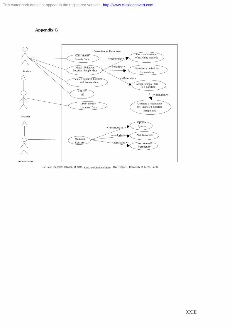
XXIII

Appendix G

Log-on/

off

Administrator

Maintain

System

Geoscience Database

<<Extends>>

<<Includes>>

Add/ Modify

Location Data

Add/ Modify

Sample Data

Assign Sample data to a Location

View Graphical Location

and Sample data

Match Unknown Location Sample data

Generate a coordinate for Unknown Location

Sample data

Generate a ranked list

For matching Student

Use combinations of matching methods

Lecturer

<<Includes>>

<<Extends>>

Update

System

Set Access Permission

s

Set Passwords

<<Includes>>

<<Includes>>

<<Includes>>

Use Case Diagram: Johnson, O 2002, UML and Rational Rose , IN21 Topic 1, University of Leeds, Leeds.



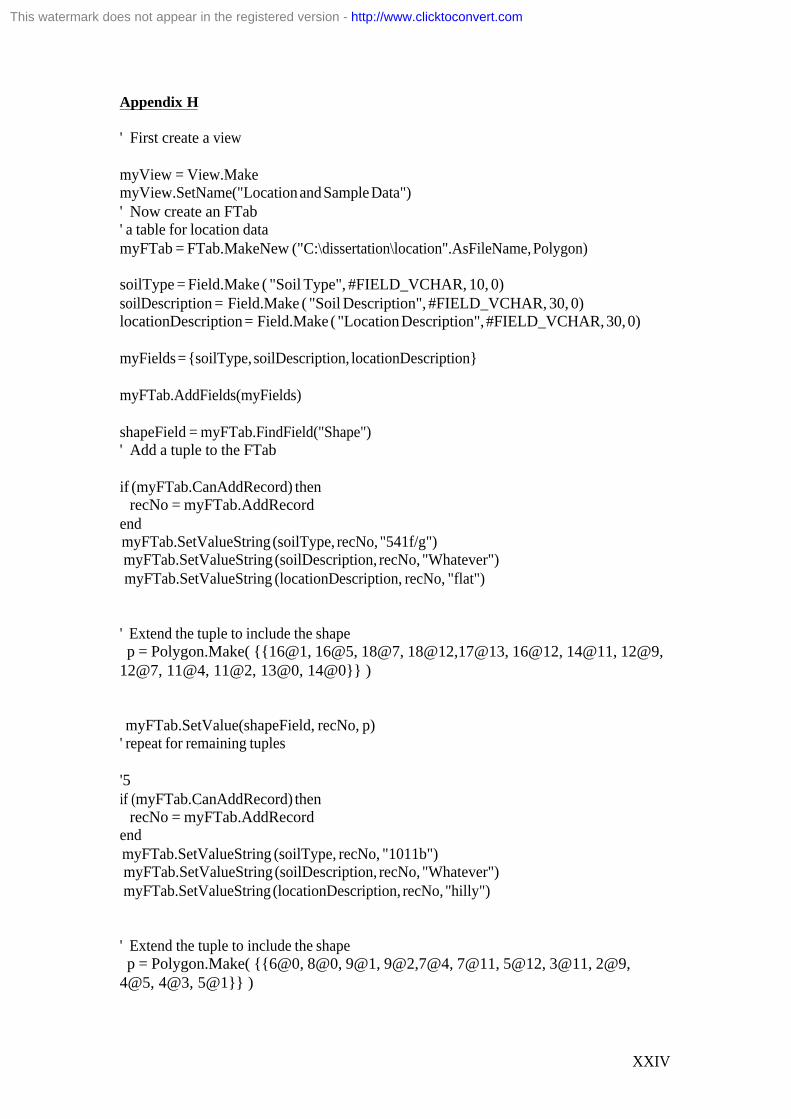
XXIV

Appendix H ' First create a view myView = View.Make myView.SetName("Location and Sample Data") ' Now create an FTab ' a table for location data myFTab = FTab.MakeNew ("C:\dissertation\location".AsFileName, Polygon) soilType = Field.Make ( "Soil Type", #FIELD_VCHAR, 10, 0) soilDescription = Field.Make ( "Soil Description", #FIELD_VCHAR, 30, 0) locationDescription = Field.Make ( "Location Description", #FIELD_VCHAR, 30, 0) myFields = {soilType, soilDescription, locationDescription} myFTab.AddFields(myFields) shapeField = myFTab.FindField("Shape") ' Add a tuple to the FTab if (myFTab.CanAddRecord) then recNo = myFTab.AddRecord end myFTab.SetValueString (soilType, recNo, "541f/g") myFTab.SetValueString (soilDescription, recNo, "Whatever") myFTab.SetValueString (locationDescription, recNo, "flat") ' Extend the tuple to include the shape p = Polygon.Make( {{16@1, 16@5, 18@7, 18@12,17@13, 16@12, 14@11, 12@9, 12@7, 11@4, 11@2, 13@0, 14@0}} ) myFTab.SetValue(shapeField, recNo, p) ' repeat for remaining tuples '5 if (myFTab.CanAddRecord) then recNo = myFTab.AddRecord end myFTab.SetValueString (soilType, recNo, "1011b") myFTab.SetValueString (soilDescription, recNo, "Whatever") myFTab.SetValueString (locationDescription, recNo, "hilly") ' Extend the tuple to include the shape p = Polygon.Make( {{6@0, 8@0, 9@1, 9@2,7@4, 7@11, 5@12, 3@11, 2@9, 4@5, 4@3, 5@1}} )



XXV

myFTab.SetValue(shapeField, recNo, p) '6 if (myFTab.CanAddRecord) then recNo = myFTab.AddRecord end myFTab.SetValueString (soilType, recNo, "1011b") myFTab.SetValueString (soilDescription, recNo, "Whatever") myFTab.SetValueString (locationDescription, recNo, "hilly") ' Extend the tuple to include the shape p = Polygon.Make( {{3@13, 4@13, 6@14, 8@16,9@15, 10@17, 10@19, 8@20, 7@21, 8@23, 9@24, 7@25, 5@25, 0@18, 1@16, 3@15, }} ) myFTab.SetValue(shapeField, recNo, p) '7 if (myFTab.CanAddRecord) then recNo = myFTab.AddRecord end myFTab.SetValueString (soilType, recNo, "711p") myFTab.SetValueString (soilDescription, recNo, "Whatever") myFTab.SetValueString (locationDescription, recNo, "hill/flat") ' Extend the tuple to include the shape p = Polygon.Make( {{26@28, 34@28, 36@29, 37@31,35@33, 36@35, 35@37, 33@36, 29@39, 27@39, 27@35, 25@34, 25@33, 23@32, 22@30 }} ) myFTab.SetValue(shapeField, recNo, p) myFTab.Flush MySrcName = SrcName.Make("C:\dissertation\location.shp") if (mySrcName <> nil) then myTheme = Theme.Make(MySrcName) myView.AddTheme(myTheme) end myFTab.Flush



XXVI

Appendix I



XXVII

Appendix J aView = av.GetProject.FindDoc("Location and Sample Data") aTheme2 = aView.FindTheme("Sample.shp") aTheme = aView.FindTheme("Location.shp") aVtab_Many = aTheme2.GetFTab aVtab_One = aTheme.GetFTab aField_Many = aVtab_Many.FindField("Shape") aField_One = aVTab_One.FindField("Shape") aVtab_Many.Join(aField_Many,aVtab_One, aField_One) aVtab_Many.Flush 'aVTab_Many.Link(aField_Many, aVTab_One, aField_One)' 'aVtab_One.Flush'



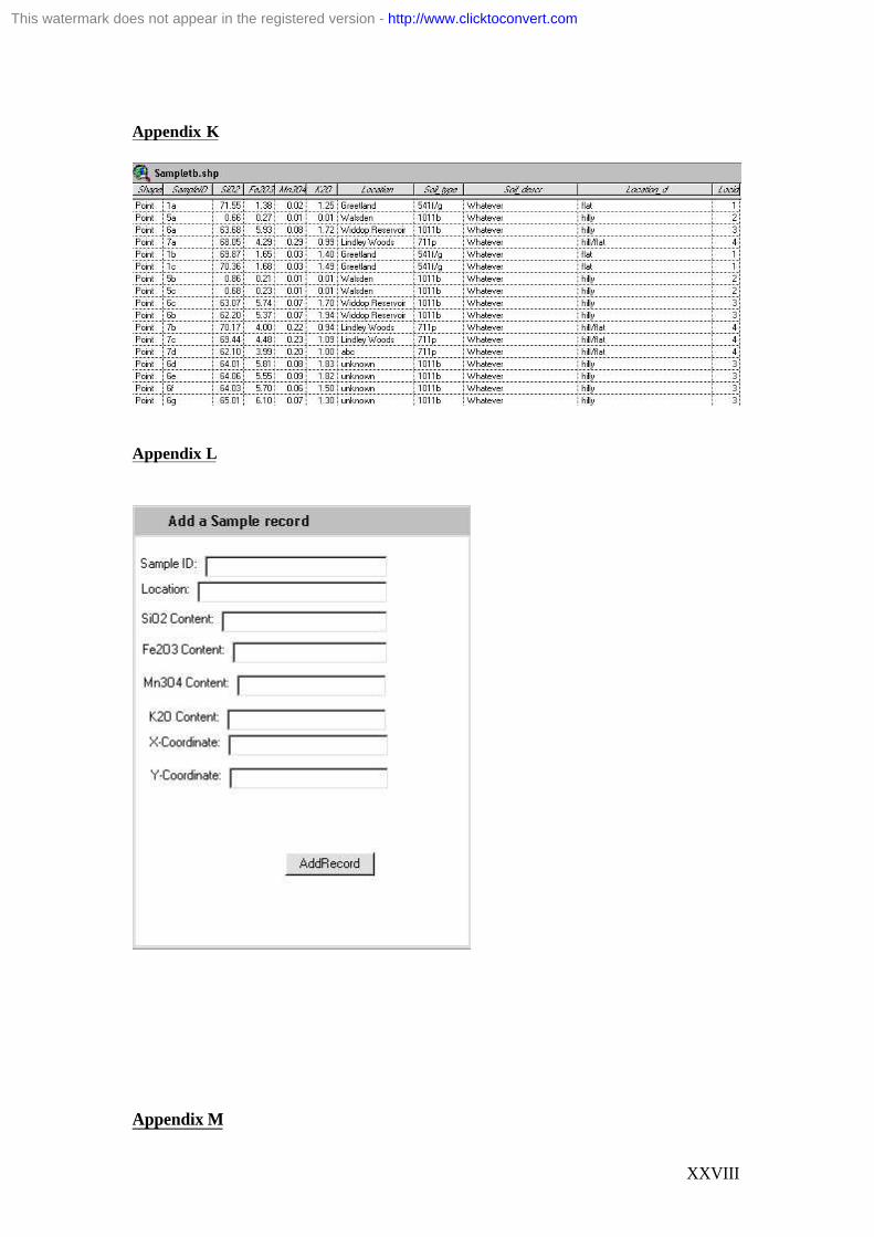
XXVIII

Appendix K

Appendix L

Appendix M



XXIX

'This code runs when the "Add Record" button is clicked ... 'SELF refers to the button '-Reference all dialog controls ... dlgAddSample = SELF.GetDialog txtSampleID = dlgAddSample.FindByName("txtSampleID") txtLocation = dlgAddSample.FindByName("txtLocation") txtSi = dlgAddSample.FindByName("txtSi") txtFe = dlgAddSample.FindByName("txtFe") txtMn = dlgAddSample.FindByName("txtMn") txtK = dlgAddSample.FindByName("txtK") txtX = dlgAddSample.FindByName("txtX") txtY = dlgAddSample.FindByName("txtY") '-Reference the VTab and all required fields ... vtbSample = dlgAddSample.GetServer fldSampleID = vtbSample.FindField("SampleID") fldLocation = vtbSample.FindField("Location") fldSi = vtbSample.FindField("SiO2") fldFe = vtbSample.FindField("Fe2O3") fldMn = vtbSample.FindField("Mn3O4") fldK = vtbSample.FindField("K2O") fldPoint = vtbSample.FindField("Shape") '-Add the new record, populate field values ... vtbSample.SetEditable(true) recNewSample = vtbSample.AddRecord vtbSample.SetValue (fldSampleID, recNewSample, txtSampleID.GetText) vtbSample.SetValue (fldLocation, recNewSample, txtLocation.GetText) vtbSample.SetValue (fldSi, recNewSample, txtSi.GetText.AsNumber) vtbSample.SetValue (fldFe, recNewSample, txtFe.GetText.AsNumber) vtbSample.SetValue (fldMn, recNewSample, txtMn.GetText.AsNumber) vtbSample.SetValue (fldK, recNewSample, txtK.GetText.AsNumber) vtbSample.SetValue (fldPoint, recNewSample, [email protected]) vtbSample.SetEditable(false) vtbSample.Refresh Msgbox.Info ("New Record Added", "Add Sample") Appendix N



XXX

'SELF refers to the dialog aView = av.GetProject.FindDoc("Location and Sample Data") aTheme = aView.FindTheme("Sample.shp") vtbSample = aTheme.GetFTab SELF.SetServer(vtbSample) Appendix O

Appendix P aView = av.GetProject.FindDoc("Location and Sample Data") aTheme = aView.FindTheme("Summary.shp") aView.DeleteTheme(aTheme) aView = av.GetProject.FindDoc("Location and Sample Data") aFTab = aView.FindTheme( "Sample.shp" ).GetFTab aFTab.SetEditable(true) lFld = aFTab.FindField( "Locid" ) siFld = aFTab.FindField( "SiO2" )



XXXI

feFld = aFTab.FindField( "Fe2O3" ) mnFld = aFTab.FindField( "Mn3O4" ) kFld = aFTab.FindField( "K2O" ) shapeFld = aFTab.FindField( "Shape" ) newFTab = aFTab.Summarize( "Summary.shp".AsFileName, Shape, lFld,{ shapeFld, siFld, siFld, siFld, feFld, feFld, feFld, mnFld, mnFld, mnFld, kFld, kFld, kFld }, { #VTAB_SUMMARY_AVG, #VTAB_SUMMARY_AVG, #VTAB_SUMMARY_MIN, #VTAB_SUMMARY_MAX, #VTAB_SUMMARY_AVG, #VTAB_SUMMARY_MIN, #VTAB_SUMMARY_MAX, #VTAB_SUMMARY_AVG, #VTAB_SUMMARY_MIN, #VTAB_SUMMARY_MAX, #VTAB_SUMMARY_AVG, #VTAB_SUMMARY_MIN, #VTAB_SUMMARY_MAX } ) aView.AddTheme( FTheme.Make( newFTab )) aFTab.SetEditable(false) Appendix Q

Appendix R aView = av.GetProject.FindDoc("Location and Sample Data") aTheme = aView.FindTheme("Summary.shp") aVtab = aTheme.GetFTab dlgMatch =av.FindDialog("Match") dlgMatch.SetServer(aVTab)



XXXII

Fefld = dlgMatch.FindByName("mtxtFe") Sifld = dlgMatch.FindByName("mtxtSi") Mnfld = dlgMatch.FindByName("mtxtMn") Kfld = dlgMatch.FindByName("mtxtK") matchLBT = dlgMatch.FindByName("mtb") Fefld.SetTextType (#TEXTLINE_TYPE_REAL) Sifld.SetTextType (#TEXTLINE_TYPE_REAL) Mnfld.SetTextType (#TEXTLINE_TYPE_REAL) Kfld.SetTextType (#TEXTLINE_TYPE_REAL) Fefld.SetText("1.57") Sifld.SetText("70.59") Mnfld.SetText("0.03") Kfld.SetText("1.38") Appendix S 'This code runs when the "Perform Match" button is clicked ... 'SELF refers to the button '-Reference all dialog controls ... dlgMatch = SELF.GetDialog aVTab = dlgMatch.GetServer aBitMap = aVTab.GetSelection Fefld = dlgMatch.FindByName("mtxtFe") Sifld = dlgMatch.FindByName("mtxtSi") Mnfld = dlgMatch.FindByName("mtxtMn") Kfld = dlgMatch.FindByName("mtxtK") cFe = dlgMatch.FindByName("cFe") cSi = dlgMatch.FindByName("cSi") cMn = dlgMatch.FindByName("cMn") cK = dlgMatch.FindByName("cK") 'match script' aListOfQueries = List.Make 'checkboxes' if (cFe.IsSelected = true) then '--- make the query string (1) ---' '--- min =< Fe2O3 >= max ---' Q1= "([Min_Fe2O3] <= " + Fefld.GetText +") " Q2= "([Max_Fe2O3] >= " + Fefld.GetText +") " aQuery = Q1 + " and " + Q2



XXXIII

aListOfQueries.Add( aQuery ) MsgBox.Info(aQuery,"") else 'aQuery = ""' 'aListOfQueries.Add( aQuery )' MsgBox.Info( "not selected", "") end if (cSi.IsSelected = true) then '--- make the query string (1) ---' '--- min =< SiO2 >= max ---' Q1= "([Min_SiO2] <= " + Sifld.GetText +") " Q2= "([Max_SiO2] >= " + Sifld.GetText +") " aQuery = Q1 + " and " + Q2 aListOfQueries.Add( aQuery ) MsgBox.Info(aQuery,"") else 'aQuery = ""' 'aListOfQueries.Add( aQuery )' MsgBox.Info( "not selected", "") end if (cMn.IsSelected = true) then '--- make the query string (1) ---' '--- min =< Mn3O4 >= max ---' Q1= "([Min_Mn3O4] <= " + Mnfld.GetText +") " Q2= "([Max_Mn3O4] >= " + Mnfld.GetText +") " aQuery = Q1 + " and " + Q2 aListOfQueries.Add( aQuery ) MsgBox.Info(aQuery,"") else 'aQuery = ""' 'aListOfQueries.Add( aQuery )' MsgBox.Info( "not selected", "")



XXXIV

end if (cK.IsSelected = true) then '--- make the query string (1) ---' '--- min =< K2O >= max ---' Q1= "([Min_K2O] <= " + Kfld.GetText +") " Q2= "([Max_K2O] >= " + Kfld.GetText +") " aQuery = Q1 + " and " + Q2 aListOfQueries.Add( aQuery ) MsgBox.Info(aQuery,"") else 'aQuery = ""' 'aListOfQueries.Add( aQuery )' MsgBox.Info( "not selected", "") end 'performing combination of queries' aList = List.Make For Each aQueryString In aListOfQueries aVTab.Query (aQueryString, aBitMap, #VTAB_SELTYPE_NEW ) aList.Add( aBitMap.Clone ) End SaveBit = aVtab.GetSelection.Clone For Each aBit In aList aVTab.SetSelection( aBit ) SaveBit.And( aVTab.GetSelection) End aVtab.SetSelection( SaveBit ) Return True Appendix T



XXXV

Appendix U Av.FindDialog("AddSample").Open Av.FindDialog("Match").Open Av.FindDialog("Menu").Open



XXXVI

Appendix V

User Manual

Contents

Section Pages

1. Open Project 2

2. Control Window 2, 3

3. Selecting a Feature and Viewing its FTab Record(s) 3

4. Selecting a Table and its Record(s) 4, 5

5. Modifying/ Deleting a Record 5, 6

6. Access to Additional Options 6, 7

7. Importing Location Data 7

8. Add Sample Data 7, 8

9. Update Match Statistics 8

10. Find a Match 8

11. Legend Editor 8



XXXVII

1. Open Project

Click on <File> then <Open Project> and select the appropriate .apr file and press <OK>.

The following screen will be displayed.

2. Control Window

If you select the <View> icon it will display the ‘Location and Sample data’ View in the

window, as demonstrated below:



XXXVIII

If double clicked the <Location and Sample data> text in the list, it will display the View and

its Theme graphically in a new window as follows:

A Theme can be selected by clicking on the area around its name. In this instance the

Location.shp Theme has been selected.

The graphical illustration of a Themes features is controlled by the Checkboxes.

3. Selecting a Feature and Viewing its FTab Record(s)

Ensure that the View window is highlighted and then select the following icon on the toolbar:

If you select a Theme and click on a Feature, a record (s) will be displayed in a table as shown

below:



XXXIX

4. Selecting a Table and its Record(s)

The Sample and Location tables are fixed and not dynamic so can be access through two

methods.

Activate the Control window and select the<Table> icon. Double click on the table from the

list that is required. For example if you click on the <Sampletb> table the following will be

displayed:

The table associated with the ‘Location’, ‘Sample’ and ‘Summary’ Themes can be accessed

through alternative means, by selecting the Theme in the View window. Then selecting the

<Theme> Menu at the top of the screen and choosing the <Table> option. This is

demonstrated below:



XL

A record can be selected by activating the Table window. Then selecting the following icon

on the toolbar:

Then select the required record.

If a record in the table is selected the associated feature in the View window will be

highlighted (providing the Theme Checkbox has been selected).

5. Modifying/ Deleting a Record

There is only a need to modify Sample data, as the Location data is imported and the

Summary data is calculated from the Sample data.

It is difficult to modify Features within a Table, so it is suggested that if amendments are to be

made to a spatial attribute the record should be deleted from the ‘Sampletb’ Table, and then

re-entered via the ‘Add Sample’ Dialog that will be discussed later.

To delete or modify a record, the record must be selected. Then the Table should be put into

edit mode by selecting the <Table> Menu at the top of the screen and choosing <Start

Editing> from the drop down list as shown below:



XLI

To delete a record select the <Edit> Menu at the top of the screen and choose <Delete

Records> from the list as illustrated below:

To modify non-spatial data in a record, select the following icon from the toolbar:

Then select the position within the Table that amendments require to be made.

On completion of deleting or modifying a record (s), the Table needs to be taken out of edit

mode to prevent accidental deletion and modification. To do this select the <Table> Menu

and choose <Stop Editing> from the list as illustrated below:



XLII

6. Access to Additional Options

Activate the Control window and select the following icon:

On selection the following Dialog will appear:

7. Importing Location Data

This option was not implemented, because data had not been acquired to import.

8. Add Sample Data

Select the <Add Sample Data> Button from the ‘Additional Options’ Dialog and this will

display the following Dialog:



XLIII

The Sample data can be entered into the respective Text-lines. The execution of the <Add

Record> button will add the record to the ‘Sampletb’ Table and thus add a point feature to the

‘Sample’ Theme. The scale of the coordinate data can be retrieved using Appendix Z.

9. Update Match Statistics

A match is found by querying data that is calculated from Sample data, so it is important to

execute the <Update Match Statistics> button on the ‘Additional options’ dialog after Sample

data has been added, modified or deleted before a match is sought.

10. Find a Match

Select the <Find a match> button from the ‘Additional Options’ Dialog. The following Dialog

will be displayed:



XLIV

The Sample data can be entered into the respective Text-lines. The fields that a match is to be

conducted upon need to have there associated Checkboxes selected. Then select the <Perform

Match> button to conduct a match. The Feature (s) that match the entered data will be

highlighted in the ‘Summary’ Theme.

11. Legend Editor Activate the View window, and double click on a Theme. Select the <Legend Type> drop down list and choose ‘Unique value’. Then select the <Values Field> drop down list and choose ‘aField’ that will group features. This will display a unique colour for each group on the Theme display.



G

Bibliography i Huggett R.J., 1975. Soil Landscape Systems: A Model of Soil Genesis. Geoderma 13: 1-22.

ii Jenny H., 1941. Factors of Soil Formation. McGraw-Hill, New York.

iii Jenny H., 1980. The Soil Resource, Origin and Behaviour, Springer-Verlag, New York

iv Arnold J.G., Allen P.M., Bernhardt G. 1993. A Comprehensive Surface-Groundwater Flow

Model. Journal of Hydrology, 142: 47-69. v White R.E., 1987. Introduction to the Principles and Practices of Soil Science. Blackwell

Scientific Publ. , Palo Alto, CA. vi

22/03/2004, Soil Horizons , http://www.michigan.gov, vii

Davidson, D & Bridges, E 1982, Principles and Application of Soil Geography , Longman,

London and New York. viii

Birkeland, P 1999, Soils and Geomorphology , 3rd edn, Oxford, New York. ix Avery B.W., 1973. Soil Classification in the Soil Survey of England and Wales. J. of Soil

Sci, 24: 324-338. x 25/03/2004, www.seasky.org/astronomy/sky1a.html

xi 25/03/2004, Loss on Ignition , http://www.ex.ac.uk/~ARAmes/loi.htm

xii 25/03/2004, www.sfaf.org/treatment/beta/b32/b32glos.html

xiii 25/03/2004, wonka.physics.ncsu.edu/~blondin/comets/help.html

xiv Gilchrist, A & Nobbs, J 1999, Colour by numbers , JSDC, Volume 115

xv 25/03/2004, www.chromalink.com/glossary.htm

xvi25/03/2004, http://www.forensicgeology.net/science.htm

xvii Glanville, D 2004, Forensic Geology, An Investigation into Soil Chemistry Fingerprinting ,

Dissertation, University of Leeds, Leeds. xviii

Bell, M 2004, Forensic Geoscience, An Investigation into Chemical Properties of Soil ,

Dissertation, University of Leeds, Leeds. xvii

Glanville, D 2004, Forensic Geology, An Investigation into Soil Chemistry Fingerprinting ,

Dissertation, University of Leeds, Leeds. xviii

Bell, M 2004, Forensic Geoscience, An Investigation into Chemical Properti es of Soil ,

Dissertation, University of Leeds, Leeds. ix Avery B.W., 1973. Soil Classification in the Soil Survey of England and Wales. J.

of Soil Sci, 24: 324-338. xviii

Bell, M 2004, Forensic Geoscience, An Investigation into Chemical Properties of Soil ,

Dissertation, University of Leeds, Leeds. xix

Rawlins, B & Cave, M 2003, Can soil geochemical survey data be used in forensic

studies? , British Geological Survey, Nottingham.



H

xx Saye, S, Wilson, H, Pye, K, Croft D & Blott, S 2003, Particle Size Determination of

Soils for Forensic Purposes using Laser Diffraction , Royal Holloway, University of

London. xxi

Croft, D, & Pye, K 2003, Colour Theory and the Evaluation of an Instrumental Method of

Measurement using Geological Samples , Kenneth Pye Associates Ltd. xix

Rawlins, B & Cave, M 2003, Can soil geochemical survey data be used in forensic

studies? , British Geological Survey, Nottingham. xxii

Johnson, O 2002, UML and Rational Rose , IN21 Topic 1, University of Leeds, Leeds xxiii

Martijn van Welie 1999-02-16 Vrije Universi teit

