Forecasting with measurement errors in dynamic models

www.elsevier.com/locate/ijforecast

International Journal of Foreca

Forecasting with measurement errors in dynamic models

Richard Harrisona,T, George Kapetaniosb, Tony Yatesa

aBank of England, UKbQueen Mary, University of London and Bank of England, UK

Abstract

In this paper, we explore the consequences for forecasting of the following two facts: first, that over time statistics agencies

revise and improve published data, so that observations on more recent events are those that are least well measured. Second,

that economies are such that observations on the most recent events contain the largest signal about the future. We discuss a

variety of forecasting problems in this environment, and present an application using a univariate model of the quarterly growth

of UK private consumption expenditure.

D 2005 Bank of England. Published by Elsevier B.V. All rights reserved.

JEL classification: C32; C53

Keywords: Forecasting; Data revisions; Dynamic models

1. Introduction There is now a large body of literature that attempts

This paper explores the consequences for forecast-

ing of two facts: first, that over time, statistics agencies

revise and (presumably) improve observations on eco-

nomic data, meaning that observations on the most re-

cent data are typically the least well measured. Second,

that economies are such that observations on the most

recent realisations of economic variables contain the

largest signal about future values of those variables.1

0169-2070/$ - see front matter D 2005 Bank of England. Published by E

doi:10.1016/j.ijforecast.2005.03.002

T Corresponding author.

E-mail addresses: [email protected]

(R. Harrison), [email protected] (G. Kapetanios),

[email protected] (T. Yates).1 See Castle and Ellis (2002, page 44) for a discussion of the

reasons why data are revised in the UK.

to examine how these facts affect forecasting and

monetary policymaking. We will not attempt a survey

in this paper, but some key strands of research are

these2: real-time data sets that enable economists to

study the properties of different vintages of data

relevant to policymaking have been compiled by

Croushore and Stark (2001) for the US, and by Castle

and Ellis (2002), Eggington, Pick, and Vahey (in

press) and Patterson and Hervai (1991) for the UK.

These works had their origins in the analyses of

preliminary and revised data by Morgenstern (1963)

and Zellner (1958). Other studies (examples are Faust,

Rogers, & Wright, 2000; Mankiw, Runkle, & Shapiro,

sting 21 (2005) 595–607

lsevier B.V. All rights reserved.

2 A helpful bibliography can be found at http://phil.frb.org/econ/

forecast/reabib.html.

http://www.phil.frb.org/econ/forecast/reabib.html



R. Harrison et al. / International Journal of Forecasting 21 (2005) 595–607596

1984; Sargent, 1989) have studied whether the

statistics agency behaves like a drationalT forecaster

by examining whether early releases of data predict

later ones. Still others have studied the implications

for monetary policy and inflation forecasts of having

to use real-time measures of important indicators like

the output gap (Orphanides, 2000; Orphanides & Van-

Norden, 2001).

Within this broad literature are papers that study

the properties of forecast models in the presence of

measurement error, and these are the closest intellec-

tual antecedents of our own. The effects of data

revisions on parameter estimates were discussed in

Denton and Okansen (1972b), Geraci (1977), and

Holden (1969). Denton and Okansen (1972a) offer

some guidance about how to conduct least squares

regression in the presence of measurement error. Cole

(1969), Denton and Kuiper (1965), and Stekler

(1967) wrote on the impact of data revisions on

forecasting. One line of enquiry has been to study a

problem of joint model estimation and signal extrac-

tion/forecasting. Optimal filters/forecasts are studied

in a line of work such as, for example, Harvey,

McKenzie, Blake, and Desai (1983) and Howrey

(1978). Koenig, Dolmas, and Piger (2003) present

informal experiments that reveal the advantages for

forecasting of using real-time data for model estima-

tion. Another focus for study has been the idea of

evaluating the properties of combinations of forecasts

(see, for example, Bates & Granger, 1969 and

discussions in Hendry & Clements, 2003). Observa-

tions on time series at dates leading up to time t are

dforecastsT of sorts of data at time t, so the problem of

how best to make use of these data is a problem of

combining forecasts.3

A brief sketch of our paper makes clear the

contribution of our work. Section 2 begins by

illustrating and proving how, in an environment when

the measurement error does not vary with the vintage,

faced with a choice between either using or not using

observations on the most recent data, it can be optimal

not to use them if the measurement error is sufficiently

large. We move on to consider a case where the more

recent the data observation, the larger the variance of

the measurement error. We find that in this case a

3 This observation is made in Busetti (2001).

many-step ahead forecast may be optimal. In Section

2.3, we generalise these results further by assuming

that the forecaster can choose the parameters of the

forecast model as well as how much of the data to use.

We find that it may be optimal to ignore recent data

and to use forecasting parameters that differ from the

parameters of the data generating process.

Section 3 generalises the results by deriving the

optimal forecasting model from the class of linear

autoregressive models. This setup allows the fore-

caster to include many lags of the data to construct the

forecast and place different weights (coefficients) on

different lags. Unsurprisingly, the optimal weighting

scheme differs from the weighting scheme that

characterises the data generating process. The greater

the signal about the future in a data point, the greater

the weight in the optimal forecasting model. More

recent and therefore more imprecisely measured data

have a smaller weight. The greater the persistence in

the data generating process, the greater the signal in

older data for the future, and the more extra measure-

ment error in recent data relative to old data makes it

optimal to rely on older data.

Throughout, this paper puts to one side the problem

of model estimation. We assume that the forecaster/

policymaker knows the true model. Taken at face

value, this looks like a very unrealistic assumption. But

it has two advantages. First, it enables us to isolate the

forecasting problem, without any loss of generality.

The second advantage is that it also emphasises an

aspect of forecasting and policy that is realistic. The

forecaster may have a noisy information source that is

contaminated with measurement error, but also con-

tains an important signal about shocks. The forecaster

may also have an information source that is not

contaminated by (at least that source of) measurement

error – an economic prior – but that does not contain

the same high frequency diagnosis of the state of the

economy. The set up we use is just an extreme version

of this. We assume that the forecaster’s prior about the

structure of the economy (the data generating process)

is correct.

In Section 4, we present an application to illustrate

the gains from exploiting the results in Section 3 using

a single-equation forecasting model for the quarterly

growth of private consumption in the UK. We use real

time data on revisions to national accounts from

Castle and Ellis (2002) to estimate how the variance

R. Harrison et al. / International Journal of Forecasting 21 (2005) 595–607 597

of measurement error declines as we move back in

time from the data frontier at T to some T�n. We find

that the optimal forecasting model does indeed use

significantly different weights on the data than those

implied by the underlying estimated model, suggest-

ing that the problem we study here may well be

quantitatively important.

2. Some issues on forecasting under data revisions

We begin, as we described in the introduction, by

illustrating how it may be optimal not to use recent

data for forecasting, but instead to rely on the model,

which we assume is known. We start with a simple

model, but we will relax some of our assumptions

later.

2.1. Age-invariant measurement error

We start with a model in which the measurement

error in an observation on an economic event is

homoskedastic and therefore not dependent on the

vintage. Assume that the true model is

yt4 ¼ ayt�14 þ et ð1Þ

where jajb1 and yt* denotes the true series. Data are

measured with error, and the relationship between the

true and observed series is given by

yt ¼ yt4þ vt : ð2Þ

For this section, we make the following assump-

tions about the processes for e and v:

etfi:i:d: 0; r2e

� �; vtfi:i:d: 0; r2

v

� �ð3Þ

which encompasses the assumption that the measured

data are unbiased estimates of the true data.4

We assume that we have a sample from period t=1

to period t=T and we wish to forecast some future

realisation yT+1* . The standard forecast (when there is

no measurement error) for yT+1* is denoted by y(0)T+1

and given by y(0)T+1=ayT : this is the forecast that

simply projects the most recent observation of yt

4 The analysis in Castle and Ellis (2002) focuses on the first

moment properties of revisions and finds some evidence of bias. But

we abstract from that issue here.

using the true model coefficient a. We investigate the

mean square properties of this forecast compared with

the general forecast y(n)T+1=an+1yT�n, a class of

forecasts that project using data that are older than

the most recent outturn.

We begin by finding an expression for the forecast

error, and then computing the mean squared error for

different forecasts amongst the general class described

above. The (true) forecast error (which of course we

never observe) is given by u(n)T+1=yT+1* �y(n)T+1. We

know that from Eq. (1) we can write:

yTþ14 ¼ anþ1yT�n4 þXni¼0

aieTþ1�i ð4Þ

and from Eq. (2) we have:

yynð ÞTþ1 ¼ anþ1yT�n ¼ anþ1yT�n4 þ anþ1vT�n : ð5Þ

So:

uunð ÞTþ1 ¼

Xni¼0

aieTþ1�i � anþ1vT�n : ð6Þ

Therefore, the mean squared error is simply given by:5

MSE nð Þ ¼ a2 nþ1ð Þr2v þ 1þ a2 � a2 nþ1ð Þ

1� a2

�r2e :

�ð7Þ

The next step is to explore the condition that the mean

squared error from a forecast using the most recent

data is less than the mean squared error that uses

some other more restricted information set, or

MSE(0) bMSE(n) for some nN0. This will tell us

whether there are circumstances under which it is

worth forecasting without using the latest data. Doing

this gives us:

MSE 0ð ÞbMSE nð ÞZ a2r2v þ r2

e b a2 nþ1ð Þr2v

þ 1þ a2 � a2 nþ1ð Þ

1� a2

�r2e

�ð8Þ

which can be written as:

r2vb

r2e

1� a2: ð9Þ

So if r2vN

r2e

1�a2it is better in terms of MSE not to use

the most recent data. The intuition is simply that if

5 Notice that this expression requires that the revision errors in Eq.

(2) are uncorrelated with future shocks to the model (1). This seems

like a reasonable assumption.


the variance of the measurement error rv2 is very

large relative to the shocks that hit the data

generating process, (re2), then it is not worth using

the data to forecast, the more this is so the smaller is

the parameter (a) that propagates those shocks. In

fact it follows that if r2vN

r2e

1�a2then MSE(n�1)N

MSE(n) for all n and therefore we are better off

using the unconditional mean of the model to

forecast the true series than any other data.

The above analysis concentrated on a simple

AR(1) model. However, the intuition is clear and is

valid for more general dynamic models.

2.2. Age-dependent measurement error

We now investigate a slightly more complex case

where the variance of the data measurement error vtis assumed to tail off over time. This assumption

reflects the observation that, in practice, we observe

that statistics agencies often revise data many times

after the first release. If we assume that successive

estimates of a particular data point are subject to

less uncertainty (since they are based on more

information), then it seems reasonable to assume

that the variance of the revision error embodied in

the estimate of a particular data point diminishes

over time.

The specific assumption we make here is that:

Var vT�ið Þ ¼ bir2v ; i ¼ 0; 1; N ;N

0; i ¼ N þ 1; N

�ð10Þ

for a parameter 0bbb1. We therefore assume that

after a finite number of periods N+1, there are no

further revisions to the data. But for the first N+1

periods, the variance of the revision error declines

geometrically over time at a constant rate measured

by b. This is a fairly specific assumption which we

make here for simplicity and tractability (again the

analysis in later sections is more general). Indeed, we

know that data are revised for reasons other than

new information specific to that series (for example

re-basing and methodology changes) so the specifi-

cation of revision error variance may be more

complicated than we have assumed here. But the

purpose of the assumption is to be more realistic

than the homoskedastic case considered in Section

2.1.

Under our assumptions, the MSE as a function of n

is given by

MSE nð Þ ¼ a2nþ2bnr2v þ

Xni¼0

a2ir2e ; n ¼ 0; 1; N ;N

ð11Þ

MSE nð Þ ¼Xni¼0

a2ir2e ¼

XNi¼0

a2ir2e þ

Xni¼Nþ1

a2ir2e ;

n ¼ N þ 1; N ð12Þ

We want to examine when MSE(n)NMSE(N+1),

n=0, 1,. . ., N. It is clear that MSE(n)NMSE(N+1),

n=N+2,. . .,. So, for n=0, 1,. . ., N

MSE nð ÞNMSE N þ 1ð ÞZ a2nþ2bnr2v

þXni¼0

a2ir2eNXni¼0

a2ir2e þ

XNþ1

i¼nþ1

a2ir2e ð13Þ

or, in terms of the signal–noise ratio, r=re2 /rv

2:

bn 1� a2ð Þ1� a2 N�nþ1ð Þ Nr2 : ð14Þ

So if Eq. (14) is true for all n, then the best

forecast for yt+1 is y(N+1)t+1 . To clarify the range

of relevant values for r we graph the quantitybnð1�a2Þ

1�a2 N�nþ1ð Þ over n for N=24, b=0.99, 0.95, 0.9, 0.5

and a=0.1, 0.3, 0.5, 0.7, 0.9 in Figs. 1–4. If each

period corresponds to one quarter, then our assump-

tion N=24 corresponds to the situation in which data

are unrevised after 6 years. While this is naturally an

approximation (since rebasing and methodological

changes can imply changes to official figures over the

entire length of the data series), it seems a plausible

one.

Clearly, the more persistent the process is (the

larger the a) the lower r2 has to be for y(N+1)t+1 to be the

best forecast. Also, the more slowly the revision error

dies out (the larger the b), the lower r2 has to be for

y(N+1)t+1 to be the best forecast. Note that some of the

curves in the figures are not monotonic. This indicates

that although y(N+1)t+1 is a better forecast than y(0)t+1, there

exists some N+1NnN0 such that y(n)t+1 is better than

y(N+1)t+1 .

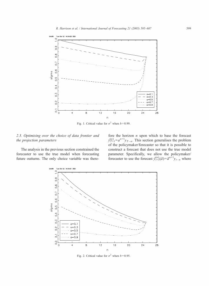
Fig. 1. Critical value for r2 when b =0.99.


2.3. Optimising over the choice of data frontier and

the projection parameters

The analysis in the previous section constrained the

forecaster to use the true model when forecasting

future outturns. The only choice variable was there-

Fig. 2. Critical value for

fore the horizon n upon which to base the forecast

y(n)T+1=an+1yT�n. This section generalises the problem

of the policymaker/forecaster so that it is possible to

construct a forecast that does not use the true model

parameter. Specifically, we allow the policymaker/

forecaster to use the forecast y(n)t+1(a)= an+1yt�n where

r2 when b =0.95.

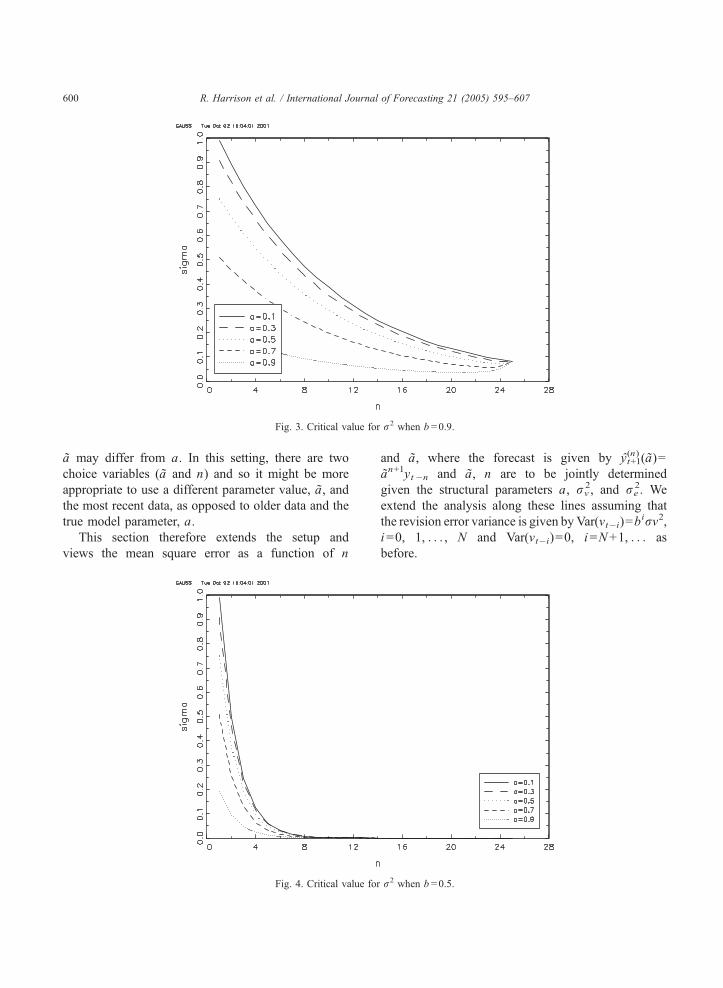
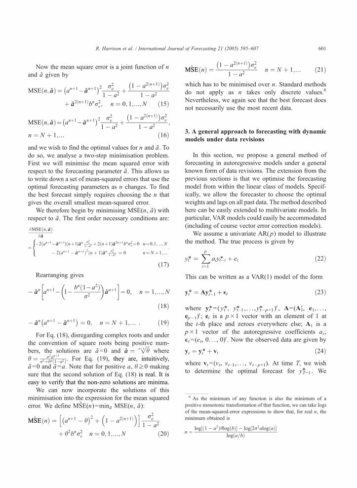
Fig. 3. Critical value for r2 when b =0.9.


a may differ from a. In this setting, there are two

choice variables (a and n) and so it might be more

appropriate to use a different parameter value, a, and

the most recent data, as opposed to older data and the

true model parameter, a.

This section therefore extends the setup and

views the mean square error as a function of n

Fig. 4. Critical value fo

and a, where the forecast is given by y(n)t+1(a)=

an+1yt�n and a, n are to be jointly determined

given the structural parameters a, rv2, and re

2. We

extend the analysis along these lines assuming that

the revision error variance is given byVar(vt�i)=birv2,

i=0, 1, . . . , N and Var(vt�i)=0, i=N+1, . . . as

before.

r r2 when b =0.5.

6 As the minimum of any function is also the minimum of a

ositive monotonic transformation of that function, we can take logs

f the mean-squared-error expressions to show that, for real n, the

inimum obtained is

¼ log½ 1� a2ð Þhlog bð Þ � log½2r2alog að Þlog a=bð Þ


Now the mean square error is a joint function of n

and a given by

MSE n; aað Þ ¼ anþ1� aanþ1� �2 r2

e

1� a2þ

1� a2 nþ1ð Þ� �r2e

1� a2

þ aa2 nþ1ð Þbnr2v ; n ¼ 0; 1; N ;N ð15Þ

MSE n; aað Þ¼ anþ1� aanþ1� �2 r2

e

1� a2þ

1� a2 nþ1ð Þ� �r2e

1� a2;

n ¼ N þ 1; N ð16Þ

and we wish to find the optimal values for n and a. To

do so, we analyse a two-step minimisation problem.

First we will minimise the mean squared error with

respect to the forecasting parameter a. This allows us

to write down a set of mean-squared errors that use the

optimal forecasting parameters as n changes. To find

the best forecast simply requires choosing the n that

gives the overall smallest mean-squared error.

We therefore begin by minimising MSE(n, a) with

respect to a. The first order necessary conditions are:

BMSE n; aað ÞBaa

¼�2 anþ1� aanþ1ð Þ nþ1ð Þaan r2

e

1�a2þ2 nþ1ð Þaa2nþ1bnr2

v¼0 n¼0;1; N ;N

� 2 anþ1 � aanþ1ð Þ2 nþ 1ð Þaan r2e

1�a2¼ 0 n¼Nþ1; N

:

8<:

(17)

Rearranging gives

� aan anþ1� 1� bn 1�a2ð Þr2

�aanþ1

� ¼ 0; n ¼ 1; N ;N

�ð18Þ

� aan anþ1 � aanþ1� �

¼ 0; n ¼ N þ 1; N : ð19Þ

For Eq. (18), disregarding complex roots and under

the convention of square roots being positive num-

bers, the solutions are a=0 and aa ¼ffiffiffihnþ1

pwhere

h ¼ r2anþ1

r2þbn 1�a2ð Þ. For Eq. (19), they are, intuitively,

a=0 and a=a. Note that for positive a, hz0 making

sure that the second solution of Eq. (18) is real. It is

easy to verify that the non-zero solutions are minima.

We can now incorporate the solutions of this

minimisation into the expression for the mean squared

error. We define MSE(n)=mina MSE(n, a):

ˆMSEMSE nð Þ ¼ anþ1 � h� �2 þ 1� a2 nþ1ð Þ

�h i r2e

1� a2

þ h2bnr2v n ¼ 0; 1; N ;N ð20Þ

ˆMSEMSE nð Þ ¼1� a2 nþ1ð Þ� �

r2e

1� a2n ¼ N þ 1; N ð21Þ

which has to be minimised over n. Standard methods

do not apply as n takes only discrete values.6

Nevertheless, we again see that the best forecast does

not necessarily use the most recent data.

3. A general approach to forecasting with dynamic

models under data revisions

In this section, we propose a general method of

forecasting in autoregressive models under a general

known form of data revisions. The extension from the

previous sections is that we optimise the forecasting

model from within the linear class of models. Specif-

ically, we allow the forecaster to choose the optimal

weights and lags on all past data. The method described

here can be easily extended to multivariate models. In

particular, VAR models could easily be accommodated

(including of course vector error correction models).

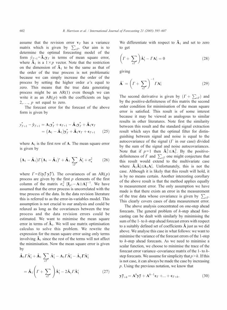
We assume a univariate AR( p) model to illustrate

the method. The true process is given by

yt4 ¼Xpi¼1

aiyt�i4 þ et ð22Þ

This can be written as a VAR(1) model of the form

yt4 ¼ Ayt�14 þ et ð23Þ

where yt*=( yt*, yt–1* , . . . ,yt�p+1* )V, A=(A1V, e1, . . . ,

ep�1)V; ei is a p�1 vector with an element of 1 at

the i-th place and zeroes everywhere else; A1 is a

p�1 vector of the autoregressive coefficients ai;

et=(et, 0. . . , 0)V. Now the observed data are given by

yt ¼ yt4þ vt ð24Þ

where vt=(vt, vt–1, . . . , vt�p+1). At time T, we wish

to determine the optimal forecast for yT+1* . We

p

o

m

n


assume that the revision error vT has a variance

matrix which is given byP

vT. Our aim is to

determine the optimal forecasting model of the

form yT+1=A1yT in terms of mean square error,

where A1 is a 1�p vector. Note that the restriction

on the dimension of A1 to be the same as that of

the order of the true process is not problematic

because we can simply increase the order of the

process by setting the higher order a’s equal to

zero. This means that the true data generating

process might be an AR(1) even though we can

write it as an AR( p) with the coefficients on lags

2, . . . , p set equal to zero.

The forecast error for the forecast of the above

form is given by

y4Tþ1 � yyTþ1 ¼ A1y4T þ eTþ1 � AA1y

4T þ AA1vT

¼ A1 � AA1

� �y4T þ AA1vT þ eTþ1 ð25Þ

where A1 is the first row of A. The mean square error

is given by

A1 � AA1

� �C A1 � AA1

� �Vþ AA1

XvT

A˜ 1Vþ r2e ð26Þ

where C=E(yT* yT* V). The covariances of an AR( p)

process are given by the first p elements of the first

column of the matrix re2 [Ip2�A�A]�1. We have

assumed that the error process is uncorrelated with the

true process of the data. In the data revision literature

this is referred to as the error-in-variables model. This

assumption is not crucial to our analysis and could be

relaxed as long as the covariances between the true

process and the data revision errors could be

estimated. We want to minimise the mean square

error in terms of A1. We will use matrix optimisation

calculus to solve this problem. We rewrite the

expression for the mean square error using only terms

involving A1 since the rest of the terms will not affect

the minimisation. Now the mean square error is given

by

AA1CA˜1Vþ AA1

XvT

A˜ 1V� A1CA˜1V� A˜ 1GA

˜1V

¼ AA1 C þXvT

!A˜ 1V� 2A˜ 1CA

˜1V

ð27Þ

We differentiate with respect to A1 and set to zero

to get�C þ

XvT

�A˜ 1V� CA1V ¼ 0 ð28Þ

giving

AAV ¼�

C þXvT

��1

CA1V ð29Þ

The second derivative is given by ðC þP

vT Þ and

by the positive-definiteness of this matrix the second

order condition for minimisation of the mean square

error is satisfied. This result is of some interest

because it may be viewed as analogous to similar

results in other literatures. Note first the similarity

between this result and the standard signal extraction

result which says that the optimal filter for distin-

guishing between signal and noise is equal to the

autocovariance of the signal (C in our case) divided

by the sum of the signal and noise autocovariances.

Note that if p=1 then A12VA1

2. By the positive-

definiteness of C andP

vT one might conjecture that

this result would extend to the multivariate case

where A1A1VVA1A1V. Unfortunately, this is not the

case. Although it is likely that this result will hold, it

is by no means certain. Another interesting corollary

of the above result is that the method applies equally

to measurement error. The only assumption we have

made is that there exists an error in the measurement

of the true data whose covariance is given byP

vT.

This clearly covers cases of data measurement error.

The above analysis concentrated on one-step ahead

forecasts. The general problem of h-step ahead fore-

casting can be dealt with similarly by minimising the

sum of the 1- to h-step ahead forecast errors with respect

to a suitably defined set of coefficients A just as we did

above. We analyse this case in what follows: we want to

minimise the variance of the forecast errors of the 1-step

to h-step ahead forecasts. As we need to minimise a

scalar function, we choose to minimise the trace of the

forecast error variance–covariance matrix of the 1- to h-

step forecasts.We assume for simplicity that pNh. If this

is not case, it can always be made the case by increasing

p. Using the previous notation, we know that

yTþh4 ¼ AhyT4þ Ah�1eT þ N þ eTþh: ð30Þ

7 For more details on the state space representation of the case we

consider see Harvey et al. (1983). There, the authors develop a state

space methodology for irregular revisions for univariate models

Multivariate models are briefly discussed as well.


So

yTþh;h4 ¼ yTþ14 ; N ; yTþh4ð Þ ¼ A hð ÞyT4 þ A h�1ð ÞeT þ N

þ eTþh;h ð31Þ

where A(h) denotes the first h rows ofAh and eT+h,h is a

vector of the first h of the vector eT+h. So the forecast

error is given by

yTþh;h4 � yyTþh;h ¼ A hð ÞyT4 þ A h�1ð ÞeT þ N

þ eTþh;h � AyAyT4 � AvAvT : ð32Þ

The part of the variance of the forecast error, depending

on A, which is relevant for the minimisation problem, is

given as before by

AA C þXvT

!AAV� 2AACA hð ÞV:

ð33Þ

Differentiating and noting that the derivative of the trace

of the above matrix is the trace of the derivative gives

tr C þXvT

!AAV� CA hð ÞV

!¼ 0:

ð34Þ

If the matrix is equal to zero, then the trace is equal to

zero and so if

C þXvT

!AAV� CA hð ÞV ¼ 0

ð35Þ

the first order condition is satisfied. But the above

equality implies that

AAV ¼ C þXvT

!�1

CA hð ÞV: ð36Þ

Finally, the variance of the optimal coefficients is easily

obtained using the Delta method.

As we see from the above exposition, our method

essentially adjusts the coefficients of the AR model to

reflect the existence of the measurement error. Of

course, using the dwrongT coefficients to forecast

introduces bias. Often, we restrict attention to best

linear unbiased (BLU) estimates. But this means that

if we have two models, one unbiased but with high

variance, and the other with a small bias but low

variance, we always pick the former. This would be

true even if the low-variance estimator had a lower

forecast MSE than the unbiased estimator. So the

reduction in variance induced by daiming offT the truecoefficients outweighs the loss from bias.

Clearly the method we suggest is optimal in terms

of mean square forecasting error conditional on being

restricted to using p periods of past data, where p=T

is a possibility. It is therefore equivalent to using the

Kalman filter on a state space model7 once p=T.

Nevertheless, the method we suggest may have

advantages over the Kalman filter in many cases.

Firstly, the method we suggest is transparent and easy

to interpret structurally. For example, one can say

something about the coefficients entering the regres-

sion and how they change when revisions occur. It is

also possible to carry out inference on the new

coefficients. We can obtain the standard errors of the

modified coefficients from the standard errors of the

original coefficients. So in forecasting, one can say

something about the importance (weight) of given

variables and the statistical significance of those

weights. From a practical point of view where a large

model with many equations is being used for

forecasting, and one which must bear the weight of

economic story-telling, one may want to fix the

coefficients for a few periods and not reestimate the

whole model. Our method has some advantages over

the Kalman filter in uses of this sort, since it just uses

the same coefficients rather than applying a full

Kalman filter every period. Finally, the method we

have is nonparametric as far as variances for the

revision error are concerned. We have a T�1 vector

of errors at time T. In the most general case, these

errors can have any T�T covariance matrix that

represents all possibilities for how the variance of

measurement error varies by vintage, over time (and,

in a multivariate setting, across variables). In other

words, our procedure allows for time variation in the

covariances, heteroscedasticity, and serial correlation.

The state space cannot easily attain that sort of

generality. In fact, a standard state space imposes

rather strict forms of covariance on the errors that are

unappealing in the context we are envisaging. These

.

Table 1

Consumption revision error standard deviations

Horizon Standard deviation

1 0.0111

2 0.0099

3 0.0085


can only be relaxed with great difficulty and by

experienced state space modellers.

Another point worth making in this context

concerns the distinction between the dnewsT and

dnoiseT alternative representations of measurement

error as discussed by, e.g., Mankiw et al. (1984) and

Sargent (1989). In this paper, we have adopted the

dnoiseT interpretation. It is worth noting that adopting

the extreme dnewsT representation where the agency

publishing data know the correct economic model and

use it to optimally filter data prior to release would

make our suggested methodology redundant for linear

models. If the published data are not equal to the truth

but are an optimal projection conditional on all

available information obtained via, say, the state

space representation of the economic model, then

the optimal forecast is obviously obtained by using

the published data in the economic model. In the

context of autoregressive models, the best one can do

is simply use the available data together with the

model, as this is equivalent to using the state space

representation.

Finally, we note that a number of practical

complications have been assumed away in the

discussion of our method. For example, the variance

of revision errors often depends not just on how long

it has been since the first release of the data, but also

on the time that data were first released. For example,

in the UK, large revisions occur once a year with the

publication of the dBlue BookT by the Office of

National Statistics.
4 0.0075
5 0.0070

6 0.0059

7 0.0048

8 0.0041

9 0.0038

10 0.0036

11 0.0034

12 0.0031

13 0.0030

14 0.0027

15 0.0024

16 0.0023

17 0.0022

18 0.0019

19 0.0019

20 0.0017

21 0.0015

22 0.0011

23 0.0007

4. Empirical illustration

We apply the general method of optimising a

forecast model to an consumption forecasting equa-

tion based on a simple AR model. Such models,

however, have been found to have very good

forecasting performance in a variety of settings. The

model is given by

Dct ¼ a0 þXpi¼1

aiDct�i þ et ð37Þ

where ct is the (log of) consumption. Many equations

of this general form include an error correction term.

However, there is significant evidence to indicate that

error correction terms may not be very helpful in a

forecasting context. Evidence presented by Hoffman

and Rasche (1996) demonstrates that the forecasting

performance of VAR models may be better than that

of error correction models over the short forecasting

horizons which concern us. Only over long horizons

are error correction models shown to have an

advantage. Christoffersen and Diebold (1998) cast

doubt on the notion that error correction models are

better forecasting tools even at long horizons, at least

with respect to the standard root-mean-square fore-

casting error criterion. They also argue that although

unit roots are estimated consistently, modelling non-

stationary series in (log) levels is likely to produce

forecasts which are suboptimal in finite samples

relative to a procedure that imposes unit roots, such

as differencing, a phenomenon exacerbated by small

sample estimation bias.

We use real time data from 1955Q1–1998Q2 for

forecasting. We use the revision data available to

provide estimates of the revision error variances. We

assume that revisions do not occur in general after 24

revision rounds. More specifically, we estimate the

data revision variances as follows: we use real time

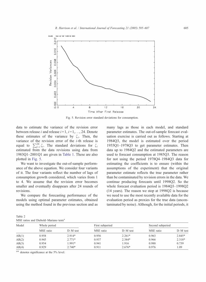
Fig. 5. Revision error standard deviations for consumption.


data to estimate the variance of the revision error

between release i and release i+1, i=1,. . ., 24. Denotethese estimates of the variance by fi. Then, the

variance of the revision error of the i-th release is

equal toP24

j¼i fi. The standard deviations for fiestimated from the data revisions using data from

1983Q1–2001Q1 are given in Table 1. These are also

plotted in Fig. 5.

We want to investigate the out-of-sample perform-

ance of the above equation. We consider four variants

of it. The four variants reflect the number of lags of

consumption growth considered, which varies from 1

to 4. We assume that the revision error becomes

smaller and eventually disappears after 24 rounds of

revisions.

We compare the forecasting performance of the

models using optimal parameter estimates, obtained

using the method found in the previous section and as

Table 2

MSE ratios and Diebold–Mariano testsa

Model Whole period First subp

MSE ratio D–M test MSE ratio

AR(1) 0.958 2.914T 0.956

AR(2) 0.945 2.771T 0.937

AR(3) 0.954 1.991T 0.941

AR(4) 0.929 2.740T 0.911

aT denotes significance at the 5% level.

many lags as those in each model, and standard

parameter estimates. The out-of-sample forecast eval-

uation exercise is carried out as follows. Starting at

1984Q3, the model is estimated over the period

1955Q1–1978Q3 to get parameter estimates. Then

data up to 1984Q2 and the estimated parameters are

used to forecast consumption at 1985Q3. The reason

for not using the period 1978Q4–1984Q3 data for

estimating the coefficients is to ensure (within the

assumptions of the experiment) that the original

parameter estimate reflects the true parameter rather

than be contaminated by revision errors in the data. We

continue producing forecasts until 1998Q2. So the

whole forecast evaluation period is 1984Q3–1998Q2

(14 years). The reason we stop at 1998Q2 is because

we need to use the most recently available data for the

evaluation period as proxies for the true data (uncon-

taminated by noise). Although, for the initial periods, it

eriod Second subperiod

D–M test MSE ratio D–M test

2.261T 0.963 2.845T2.384T 0.966 2.318T1.916 0.988 0.739

2.676T 0.976 1.09

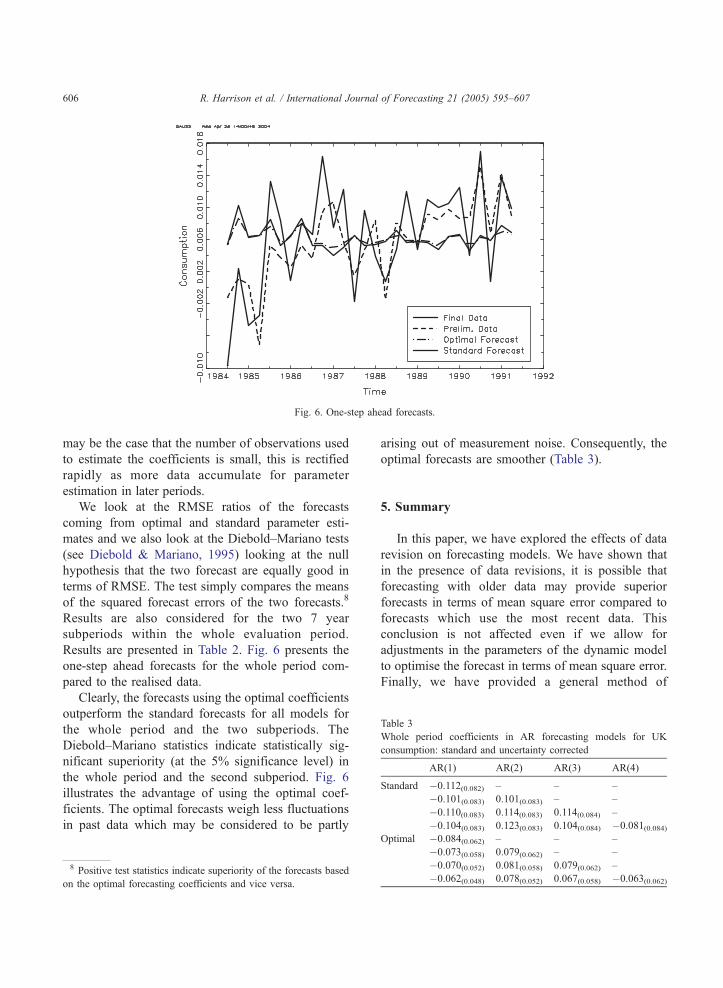
Fig. 6. One-step ahead forecasts.

Table 3

Whole period coefficients in AR forecasting models for UK

consumption: standard and uncertainty corrected

AR(1) AR(2) AR(3) AR(4)

Standard �0.112(0.082) – – –

�0.101(0.083) 0.101(0.083) – –

�0.110(0.083) 0.114(0.083) 0.114(0.084) –

�0.104(0.083) 0.123(0.083) 0.104(0.084) �0.081(0.084


may be the case that the number of observations used

to estimate the coefficients is small, this is rectified

rapidly as more data accumulate for parameter

estimation in later periods.

We look at the RMSE ratios of the forecasts

coming from optimal and standard parameter esti-

mates and we also look at the Diebold–Mariano tests

(see Diebold & Mariano, 1995) looking at the null

hypothesis that the two forecast are equally good in

terms of RMSE. The test simply compares the means

of the squared forecast errors of the two forecasts.8

Results are also considered for the two 7 year

subperiods within the whole evaluation period.

Results are presented in Table 2. Fig. 6 presents the

one-step ahead forecasts for the whole period com-

pared to the realised data.

Clearly, the forecasts using the optimal coefficients

outperform the standard forecasts for all models for

the whole period and the two subperiods. The

Diebold–Mariano statistics indicate statistically sig-

nificant superiority (at the 5% significance level) in

the whole period and the second subperiod. Fig. 6

illustrates the advantage of using the optimal coef-

ficients. The optimal forecasts weigh less fluctuations

in past data which may be considered to be partly

8 Positive test statistics indicate superiority of the forecasts based

on the optimal forecasting coefficients and vice versa.

arising out of measurement noise. Consequently, the

optimal forecasts are smoother (Table 3).

5. Summary

In this paper, we have explored the effects of data

revision on forecasting models. We have shown that

in the presence of data revisions, it is possible that

forecasting with older data may provide superior

forecasts in terms of mean square error compared to

forecasts which use the most recent data. This

conclusion is not affected even if we allow for

adjustments in the parameters of the dynamic model

to optimise the forecast in terms of mean square error.

Finally, we have provided a general method of

Optimal �0.084(0.062) – – –

�0.073(0.058) 0.079(0.062) – –

�0.070(0.052) 0.081(0.058) 0.079(0.062) –

�0.062(0.048) 0.078(0.052) 0.067(0.058) �0.063(0.062

)

)


determining the optimal forecasting model in the

presence of data measurement and revision errors with

known covariance structure. An empirical illustration

on forecasting consumption was also considered.

Acknowledgements

This paper represents the views and analysis of the

authors and should not be thought to represent those

of the Bank of England or Monetary Policy Commit-

tee members. We would like to thank the editor and

two anonymous referees for their suggestions and

help.

References

Bates, J. M., & Granger, C. J. W. (1969). The combination of

forecasts. Operational Research Quarterly, 20, 133–167.

Busetti, F. (2001). The use of preliminary data in econometric

forecasting: An application with the Bank of Italy Quarterly

Model , Bank of Italy Discussion Paper.

Castle, J., & Ellis, C. (2002, Spring). Building a real-time database

for GDP(E). Bank of England Quarterly Bulletin, 42–49.

Christoffersen, P., & Diebold, F. (1998). Co-integration and long-

horizon forecasting. Journal of Business and Economic Sta-

tistics, 16, 450–458.

Cole, R. (1969). Data errors and forecasting accuracy. In Jacob

Mincer (Ed.), Economic forecasts and expectations: Analyses of

forecasting behaviour and performance. New York7 NBER.

Croushore, D., & Stark, T. (2001). A real time data set for

macroeconomists. Journal of Econometrics, 105, 111–130.

Denton, F., & Kuiper, J. (1965). The effect of measurement errors

on parameter estimates and forecasts. Review of Economics and

Statistics, 47, 198–206.

Denton, F., & Okansen, E. (1972a). Data uncertainties and least

squares regression. Applied Statistics, 21(2), 185–195.

Denton, F., & Okansen, E. (1972b). A multi-country analysis of the

effects of data revisions on an econometric model. Journal of

the American Statistical Association, 67, 286–291.

Diebold, F. X., & Mariano, R. S. (1995). Comparing predictive

accuracy. Journal of Business and Economic Statistics, 13,

253–263.

Eggington, D., Pick, A., & Vahey, S. (in press). Keep it real!: A real-

time data set for macroeconomists: Does the vintage matter?

Economics Letters.

Faust, J., Rogers, J., & Wright, J. (2000). News and noise in G-7

GDP announcements, Federal Reserve Board of Governors

International Finance Discussion Papers, no. 690.

Geraci, V. J. (1977). Estimation of simultaneous equation models

with measurement error. Econometrica, 45(5), 1243–1255.

Harvey, A., McKenzie, C. R., Blake, D. P. C., & Desai, M. J.

(1983). Irregular Data Revisions. In A. Zellner (Ed.), Proceed-

ings of ASA-CENSUS-NBER Conference on Applied Time Series

Analysis of Economic Data (pp. 329–347). Washington, DC7

US Department of Commerce.

Hendry, D. F., & Clements, M. P. (2003). Economic forecasting:

Some lessons from recent research. Economic Modelling, 20,

301–329.

Hoffman, D. L., & Rasche, R. H. (1996). Assessing forecast

performance in a cointegrated system. Journal of Applied

Econometrics, 11, 495–517.

Holden, K. (1969). The effect of revisions to data on two

econometric studies. Manchester School, 37, 23–37.

Howrey, E. P. (1978). The use of preliminary data in econometric

forecasting. Review of Economic Statistics, 60, 193–200.

Koenig, E. F., Dolmas, S., & Piger, J. (2003). The use and abuse of

real-time data in economic forecasting. Review of Economics

and Statistics, 85, 618–628.

Mankiw, N. G., Runkle, D. E., & Shapiro, M. D. (1984). Are

preliminary estimates of the money stock rational forecasts?

Journal of Monetary Economics, 14, 14–27.

Morgenstern, O. (1963). On the accuracy of economic observations.

Princeton7 Princeton University Press.

Orphanides, A. (2000). The quest for prosperity without inflation,

Sveriges Riksbank working paper number 93.

Orphanides, A., & Van-Norden, S. (2001). The reliability of

inflation forecasts based on output gaps in real time, mimeo.

Patterson, K. D., & Hervai, S. M. (1991). Data revisions and

expenditure components of GDP. Economic Journal, 101,

887–901.

Sargent, T. J. (1989). Two models of measurement and the

investment accelerator. Journal of Political Economy, 97,

251–287.

Stekler, H. O. (1967). Data revisions and economic forecasting.

Journal of the American Statistical Association, 62, 470–483.

Zellner, A. (1958). A statistical analysis of provisional estimates of

Gross National Product and its components, of selected national

income components, and of personal savings. Journal of the

American Statistical Association, 52, 54–65.

Richard Harrison is a Senior Economist in the Monetary Assess-

ment and Strategy Division, Bank of England.

George Kapetanios is Professor of Economics at Queen Mary,

University of London and a Consultant at the Bank of England. He

has previously worked for the National Institute for Economic and

Social Research.

Tony Yates is a Manager in the Monetary Assessment and Strategy

Division, Bank of England.

Documents

Forecasting with measurement errors in dynamic models