Forecasting the Volatility of the Chinese Gold Market by

HAL Id: hal-01709321https://hal.archives-ouvertes.fr/hal-01709321

Preprint submitted on 14 Feb 2018

HAL is a multi-disciplinary open accessarchive for the deposit and dissemination of sci-entific research documents, whether they are pub-lished or not. The documents may come fromteaching and research institutions in France orabroad, or from public or private research centers.

L’archive ouverte pluridisciplinaire HAL, estdestinée au dépôt et à la diffusion de documentsscientifiques de niveau recherche, publiés ou non,émanant des établissements d’enseignement et derecherche français ou étrangers, des laboratoirespublics ou privés.

Forecasting the Volatility of the Chinese Gold Market byARCH Family Models and extension to Stable Models

Marie-Eliette Dury, Bing Xiao

To cite this version:Marie-Eliette Dury, Bing Xiao. Forecasting the Volatility of the Chinese Gold Market by ARCHFamily Models and extension to Stable Models. 2018. �hal-01709321�

https://hal.archives-ouvertes.fr/hal-01709321

https://hal.archives-ouvertes.fr

Marie-Eliette Dury, Bing Xiao 1

Forecasting the Volatility of the Chinese Gold Market by ARCH Family Models and

extension to Stable Models

Marie-Eliette DURY

School of Economics, Clermont Auvergne University

France

[email protected]

Bing XIAO

University Technology Institute (IUT), Aurillac

CRCGM EA 38 49 Clermont Auvergne University

France

[email protected]

Abstract

Gold plays an important role as a precious metal with portfolio diversification; also it is an

underlying asset in which volatility is an important factor for pricing option. The aim of this

paper is to examine which autoregressive conditional heteroscedasticity model has the best

forecast accuracy applied to Chinese gold prices. It seems that the Student’s t distribution

characterizes better the heavy-tailed returns than the Gaussian distribution. Assets with higher

kurtosis are better predicted by a GARCH model with Student’s distribution while assets with

lower kurtosis are better forecasted by using an EGARCH model. Moreover, stochastic

models such as Stable processes appear as good candidates to take heavy-tailed data into

account. The authors attempt to model and forecast the volatility of the gold prices at the

Shanghai Gold Exchange (SGE) during 2002–2016, using various models from the ARCH

family. The analysis covers from October 30, 2002 to December 7, 2015 and from December

8, 2015 to May 6, 2016 as in-sample and out-of-sample sets respectively. The results have

been estimated with MAE, MAPE and RMSE as the measures of performance.

Keywords: Forecasting, Return, Volatility, Gold Market, ARCH, GARCH, GARCH-M,

IGARCH, NGARCH, EGARCH, PARCH, NPARCH, TARCH, Student’s t distribution,

Symmetric Stable models, H-self-similar processes

JEL Classification: C53, C58, G17


1. Introduction

Gold is a precious metal which forms an integral part of many investment portfolios; it has

similar characteristics to money (see Solt and Swanson, 1981). Ciner (2001) indicates that

gold plays an important role as a precious metal with portfolio diversification properties:

holding gold leads to a more balanced portfolio. Lawrence (2003) finds that gold returns are

less correlated with returns on equities and bonds than other assets. Many researchers and

professionals believe that gold plays the role of a hedge against inflation. Sjaastad and

Scacciavillani (1996) claim that gold is a refuge value against inflation. Central banks and

international financial institutions hold a large proportion of gold for their diversification

capacity, and gold is considered as an insurance against market crises. According to Smith

(2002), when the economic environment becomes more uncertain, gold plays a role as a safe

haven. A number of authors have reported the fact that gold reflects the value of the US

dollar, because a depreciation in the dollar may increase interest in gold, Tully and Lucey

(2007) report that a lower US dollar makes gold less expensive for other international

investors to buy dollar-denominated gold.

The Chinese assets market is one of the emerging assets markets which offer an opportunity

for international diversification. Since the 1990s, reforms in regulations as well as in the

attitudes of regulators have rendered the stock market more efficient. However, it would seem

that in the Chinese assets market, anomalies persist (see Mookerjee and Yu, 1999; Mitchell

and Ong, 2006). This article studies the volatility of gold prices in China through gold prices

at the Shanghai Gold Exchange (SGE). As mentioned in Hoang et al. (2015), it is important to

use local gold prices when studying the Chinese gold market since it is still forbidden for

Chinese investors to trade gold abroad without authorization.

It has become more important for financial institutes to consider the volatility of a financial

asset. The movements are usually measured by the volatility and can be seen as the risk of the

asset. One of the problems with modelling the volatility is that it is non-stationary: there are

periods with low movements and then periods with high movements. The first model that

assumed that volatility is not constant is ARCH (autoregressive Conditional

Heteroscedasticity Model) by Engle in 1982. The ARCH model has been transformed and

developed into more sophisticated models, such as GARCH, EGARCH, PARCH and

TARCH. The questions to ask are: Do the new models capture the volatility better? If one


model better captures the volatility, would it lead to a more efficient forecast accuracy?

Currently, results of research into the model’s performance are conflicting and confusing.

These observations lead the author to determine how well these different models perform in

terms of forecasting volatility and will be assessed based on the forecasts they produce. This

study focuses on the gold prices at the Shanghai Gold Exchange (SGE); it contributes to the

existing finance literature by investigating the Chinese gold market during the recent period.

In addition, this work opens another suitable way to model heavy-tailed data, such as returns.

Heavy-tailed data can be modelled very well by α-Stable distributions because of the high

variability of the data.

The structure of this article is as follows. Section 2 provides a brief overview of the existing

literature. Data and methodology are described in Section 3 which firstly recalls the different

ARCH Family models. Then, construction and properties of Symmetric α-Stable processes

are presented; the aim is to show the adequacy of this model in this context. Next, Section 4

displays the results of this study with the numerical comparison between Student and

Gaussian distribution.

2. Literature Review

Engle’s (1982) study was the first to distinguish between unconditional and conditional

variance. According to the ARCH models, the variance of the current error term is a function

of the previous time period’s error terms. Bollerslev (1986) points out that the ARCH model

has a long lag in the conditional variance equation. To avoid problems of negative variance

parameter estimates, his solution was to generalize the ARCH model. Nelson (1991) proposed

the EGARCH model to account for the presence of asymmetric effects. Poon and Granger

(2003) noted that models that allowed for asymmetric effects are able to provide better

forecasts owing to the negative relationship between volatility and shocks.

Most research on volatility modeling has focused on equity markets and foreign exchange

markets, but Sadorsky (2006) pointed out that one type of market cannot be generalized

across other markets. It seems that stocks with higher kurtosis were better predicted by using

the GARCH model and stocks with lower kurtosis were forecasted better by using EGARCH.


Ederington and Guan (2005) showed that the financial market has a longer memory than

explained by the GARCH(1,1) model. Awrtani and Corradi (2005) found that the asymmetric

models perform better than the GARCH(1,1) model. After comparing the different volatility

models, Köksal (2009) found that the EGARCH(1,1) performed best. Bracker and Smith

(1999) studied the volatility of the copper futures market, and concluded that both the

GARCH and EGARCH models best fit this market’s volatility. Carvalho et al. (2006) found

evidence of asymmetric effects when using the EGARCH model.

However, not all the empirical studies agree with these findings. Ramasamy and Munisamy

(2012) found that the GARCH models are better to predict the volatility of exchange rates and

the EGARCH model does not improve the quality of the forecasts. Marcucci (2005) found

that the GARCH model performs much better than other models in a long time period, but not

in a short time period. Zahangir et al. (2013) investigated the ARCH models for forecasting

the volatility of equity returns. Their study showed that based on in-sample statistical

performance, both the ARCH and PARCH models are considered the best performing model

whereas all models except the GARCH and TARCH models are regarded as the best model

for the returns series.

3. Data and Methodology

The main motive of this paper is to investigate the use of the ARCH family models for

forecasting the volatility of the Shanghai Gold Exchange (SGE) by using daily data. GARCH,

EGARCH, PARCH, IGARCH, GARCHM and TARCH models are used for this study.

3.1 Data

The data used is the returns on the Shanghai Gold Exchange (SGE) returns series (Figure 1).

In order to calculate these returns, we use data on the daily price. Data on prices spans the

period from October 30, 2002 to May 6, 2016, a total of 3,278 observations. The total data set

is divided into in-sample samples and out-of-sample samples. The requisite data is obtained

from the Factset database. The price taken as the daily price is the last trading price of the

day.

Figure 1 shows the gold prices at the Shanghai Gold Exchange (SGE) from October 2002 to

May 2016, the crash of 2007 is clearly visible as well as the major long-run rise in the index

in 2002-2011. The index is non-stationary, since its mean level is not constant and rises over


time. The daily return on the index appears to be stationary with a constant mean and

variance. The outliers, namely very large or very small returns, imply that the returns are non-

normal with fat tails and the distribution may be asymmetric.

Figure 1: Chines gold market prices and returns (Daily, 2002 – 2016)

A positive skewness of 0.11876799 and negative kurtosis of -1.04121692 are revealed in the

gold price summary statistics at the Shanghai Gold Exchange (SGE) (Table A1 in the

Appendix). At a confidence interval of 99%, the SGE Index is non-normal, in accordance

with Jarque-Bera statistics. Therefore, it is necessary to remodel the gold price series into a

return series. Plotting autocorrelation and partial autocorrelation of the SGE index designates

the series to be non-stationary (Figures A1 and A2 in the Appendix). Applying the Dickey-

Fuller test and the Phillips-Perron test to the series confirms this (Table A2, A3 in the

Appendix), and suggests that it cannot be used to model volatility.

Movements of stock indices series are not suitable for study as they are usually non-stationary

and it is therefore necessary to remodel the daily price into a return series. The SGE index

series is converted into a returns series by using the following equation:

�� = � �� − 1 (1.1)

The logarithm of the gross return is given by:

-15,00%

-10,00%

-5,00%

0,00%

5,00%

10,00%

15,00%

0

50

100

150

200

250

300

350

400

450

30

/10

/20

02

15

/05

/20

03

17

/11

/20

03

21

/05

/20

04

23

/11

/20

04

08

/06

/20

05

13

/12

/20

05

26

/06

/20

06

27

/12

/20

06

11

/07

/20

07

17

/01

/20

08

04

/08

/20

08

17

/02

/20

09

19

/08

/20

09

03

/03

/20

10

06

/09

/20

10

22

/03

/20

11

22

/09

/20

11

09

/04

/20

12

15

/10

/20

12

24

/04

/20

13

06

/11

/20

13

15

/05

/20

14

19

/11

/20

14

28

/05

/20

15

03

/12

/20

15

Close prices Return prices


� �� = ln� �� (1.2)

Where,

��= the rate of return at time t

�� = the price at time t

�� = the price just prior to the time t

Statistics on returns are summarized in Table 1, where the SGE index has a 0.04 average daily

return and a 0.000208 standard deviation. At -0.05748, the skewness coefficient is negative

which is common for most financial time series. The kurtosis value is higher than 3, implying

that the returns distribution has fat tails. The ARCH family of models should, therefore, be

used to account for these characteristics of the data. When modelling a series of this sort, it

must be stationary and the data must be mean-reverting. Therefore, the Dickey-Fuller test is

used on the returns series (Table A4 in the Appendix) to confirm that the series is, indeed,

stationary. The Phillips-Perron test can also be applied to confirm that the series is stationary

and, in addition, for modelling (Table A5 in the Appendix).

Table 1: Summary statistics for returns

Observations Mean Standard Deviation Min Max Skewness Kurtosis

Returns 3278 0.0004 0.00020864 -0.103765 0.127962 -0.05748 14.00012

The observed pattern in Figure 1 indicates that GARCH type models are necessary to model

return volatility patterns for SGE index returns. The return volatility descriptive statistics

presented in Table 1 indicate a Kurtosis at 14.00012. Since the Kurtosis statistic is greater

than three, the SGE return series is leptokurtic (Figure2).


Figure 2: Leptokurtic distribution of SGE return series

According to recent research, it seems that returns with higher kurtosis were better predicted

by using GARCH with student’s distribution and returns with lower kurtosis were forecasted

better by using EGARCH. Skewness is -0.05748, this indicates that return volatiles are

negatively skewed (left skewness). Negative skewness indicates that the upper tail of

distribution is thinner than the lower tail. That indicates that in the SGE market, prices fall

more often than they rise. The ADF-test, as well as the PP-test, are used to get confirmation

regarding whether the return series is stationary or not. The value of the ADF test statistic, -

62.283, is less than its test critical value, -3.410, at 5%, level of significance, which implies

that the gold price return series is stationary. The findings of the PP test also confirm that the

return series is stationary, since the values of the PP test statistic is less than its test critical

value. The plotted autocorrelation and partial autocorrelation of squared returns indicate

dependence and hence imply a time-varying volatility (Figures A3 and A4 in the Appendix).

3.2 Specification of the Models used in this study

In order to model the volatility of the returns, we need to determine their mean

equation. The return for today will depend on returns in previous periods (autoregressive

component) and the surprise terms in previous periods (moving order component). In this

empirical study, plotting the autocorrelation and partial autocorrelation of the returns series

can help determine the order of the mean equation.

Leptokurtic

SGE return series

Gaussian

Distribution

Mean: 0.0004

SD: 0.00020864

0

0,02

0,04

0,06

0,08

0,1

0,12

0,14

0,16

0,18

-6,7

6%

-6,1

6%

-5,5

6%

-4,9

6%

-4,3

6%

-3,7

6%

-3,1

6%

-2,5

6%

-1,9

6%

-1,3

6%

-0,7

6%

-0,1

6%

0,4

4%

1,0

4%

1,6

4%

2,2

4%

2,8

4%

3,4

4%

4,0

4%

4,6

4%

5,2

4%

5,8

4%

6,4

4%

7,0

4%

7,6

4%

8,2

4%

Observations Normal Distribution


Like most financial time series, the returns series exhibits what is referred to as “volatility

clustering” (Figures A5 and A6 in the Appendix). In order to model such patterns of behavior,

the variance of the error term is allowed to depend on its history. The classic model of such

behavior is the ARCH model introduced by Engle (1982), which simultaneously models the

mean and variance of a series.

3.2.1 ARCH(q) model

Autoregressive conditional heteroscedasticity (ARCH) models are used when the error terms

will have a characteristic size or variance. The ARCH models assume the variance of the

current error term to be a function of the actual sizes of the previous time period’s error terms.

The ARCH model is a non-linear model which does not assume the variance is constant. The

basic linear ARCH model may be presented as:

�� = �� + �. (2)

The error terms are split into a stochastic piece and a time dependent standard deviation:

�� = �� (3)

The random variable is a white noise process, the series �� is the volatility of the time series

which changes over time, and �� (variances of the residual) is modelled by:

�� = � + �� +⋯+ �"��"� = � + ∑ �$"$%� ��$� (4)

Where � > 0� (�$ > 0. 3.2.2 GARCH(p, q) model

The GARCH model is a generalized ARCH model, developed by Bollerslev (1986) and

Taylor (1986) independently. They introduced a moving average term into the ARCH

estimation. A fixed lag structure is imposed. The GARCH(p, q) model, where p is the order of

the GARCH terms �� and q is the order of the ARCH terms ��.

�� = * + �� +⋯+ �"��"� + +�� +⋯+ +,��,�

= * +∑ �$"$%� ��$� +∑ +$,$%� ��$� (5)


The form of GARCH(1,1) is given below, the equation (5) is the conditional variance

equation, �� is the one period forecast variance based on past information, �� is determined

by � , �� and �� . Where the news about volatility from the previous period is �� ,

measured as the lag of the squared residual from the equation (2), and �� is used to be

considered as the last period’s (forecast) variance.

�� = � + �� + +�� (6)

Engle and Bollerslev (1986) indicated that the coefficient �- + +� measures the volatility

shock, when �- + +� is closed to one, the volatility shocks are persistent, this means that the

volatility may take long time to return to a quieter phase.

3.2.3 GARCH-M model

The M in GARCH-M stands for “in the mean”. This model is an alternative ARCH model

developed by Engle and Bollerslev (1986). GARCH-M is used when the expected financial

time series return is related to the expected asset risk. The conditional variance is included in

the conditional mean equation. The GARCH-M (1,1) is written as:

.� = /0�1��2 + 3�� + �� (7)

�� = �� The equation shows that the returns (.��has a positive relation to its own volatility. Engle and

Bollerslev proposed to introduce the logarithm of conditional variance into the mean

equation; the equation (7) can be expressed as:

�� = �� + 4 log�� + �� (8)

3.2.4 IGARCH

Consider the GARCH model in ARMA equation:

�� = �� = � + ∑ �$��$�"$%� + ∑ +7��7�,7%� (9)


Where the parameter α is the ARCH parameter and β is the GARCH parameter, α(L) and β(L)

is defined polynomials, and � > 0, �$ ≥ 0, +$ ≥ 0� ( ∑ ��$ + +$� < 1;<=�,,"�$%� .

3.2.5 EGARCH model

The EGARCH model was developed by Nelson (1991) as a solution to avoid problems with

negative variance parameter estimates. If “bad news” has a more pronounced effect on

volatility than “good news” of the same magnitude, then a symmetric specification such as

ARCH or GARCH is not appropriate since in standard ARCH/GARCH models the

conditional variance is unaffected by the sign of the past periods’ errors (it depends only on

squared errors). The logarithmic function ensures that the conditional variance is positive

and, therefore, the parameters can be allowed to take negative values. The form of

GARCH(1,1) is given below:

log �� = * + + log �� + > ?��@A��B + �C |?��|

@A��B −@2 FG H (10)

According to Engle and Ng. (1993), the EGARCH model allows positive return shocks and

negative return shocks so that there are different effects on volatility; the coefficient >

measures the asymmetry effect. Gokan (2000) indicated that when > = 0, the goods news

(positives return shocks) has the same effect on volatility as bad news represents the negative

return shocks.

In equation (10), positive return shocks, namely good news, has �* + >� impacts on return

volatility while the negative return shocks, bad news, has a �* − >� impacts. If * and > are

positive, the good news will have more effect on return than bad news. According to previous

studies in this subject, the coefficient > is often negative; this suggests negative return shocks

have more impact on return volatility than good news.

3.2.6 PARCH model

The PARCH model is a GARCH model with an additional term to account for the

asymmetries effect. It employs an indicator function as follows (PARCH(1, 1)):

�� = � + �� + +�� + >�� I�� (11)


The indicator function takes a value of 1 if the error > 0, and 0 otherwise. For the effect of the

previous period’s bad news to be greater than the effect of good news of the same magnitude,

γ should be significant and have a negative sign.

3.2.7 TARCH model

The Threshold GARCH (TARCH) model by Zakoïan (1994) is one on conditional standard

deviation instead of conditional variance. The effect of good and bad news is captured

separately through the two coefficients, α and γ, respectively. The TARCH model adds a

separate variable for negative shocks.

�� = * + ∑ �$��$�"$%� + ∑ +7��7�,7%� + ∑ >J��J� I��JKJ%� (12)

I��JLLLLL equals one if � is less than zero and zero if else. The form of TARCH(1,1) is given below:

�� = * + �� + +�� + >�� I��LLLLL (13)

In equation (12) and (13), good news (positive return shocks) and bad news (�� < 0) have

different impacts on the conditional variance. Positive return shocks have an --effect on

volatility, while bad news has an (- + >)-effect on the conditional variance (volatility). If >

equals zero, the TARCH model becomes a linear GARCH (symmetric) model. If > ≠ 0, then

that suggests an asymmetric effect.

3.2.8 NGARCH model

Nonlinear GARCH (NGARCH) is known as nonlinear asymmetric GARCH(1,1).

�� = � + �� − N�� + +�� (14)

��, + ≥ 0; � > 0

For the return series, parameter φ is positive, it means a leverage effect: negative returns

increase future volatility by a larger amount than positive returns of the same magnitude.

3.2.9 Student’s t distribution

One of the problems with forecasting volatility is the distribution: there are periods with low

movements and periods with high movements. Köksal (2009) indicates that the Student’s t

distribution characterizes better the heavy-tailed returns than the Gaussian distribution. It


seems that stocks with higher kurtosis were better predicted by using GARCH with student’s

distribution and stocks with lower kurtosis were better forecasted by using EGARCH model

(see Grek A., 2014).

In the ARCH models, the first part is �� = �� with P�~R�0,1�. In the GARCH model with

student distribution, the first part is written as part �� = ��.� with ��~S�(� and ( is the

degrees of freedom.

3.2.10 Extension to Stable Models

The most famous stochastic model for self-similar phenomena is certainly the Fractional

Brownian Motion (fBm) popularized by Benoit Mandelbrot in the 60’s. The fractional

Brownian motion is the only H-self-similar centered Gaussian process with stationary

increments in dimension 1. There exist several generalizations of the fractional Brownian

motion, such as the multifractional Brownian motion (mBm) defined independently by Peltier

and Lévy-Véhel, and by Benassi et al.

Such Gaussian models are well known and applied in different fields. Nevertheless, as soon as

the observed phenomenon has large fluctuations or high variability, they are no longer

appropriate. Such limitations lead us to propose stable non-Gaussian models as those data

present large fluctuations and variability on the collected values.

The stable non-gaussian framework is however much more complicated than the Gaussian

one. It is richer as there exist at least two distinct models of H-self-similar symmetric α-stable

(SαS) family of processes: the so-called Moving Average and the Harmonizable stable

process. Actually, they are distinct since they form two disjoint classes of processes, as

proved in Cambanis et al. and in the reference book of Samorodnitsky and Taqqu. In the

Gaussian case where - = 2, the two classes describe in fact the same, since they have the

same law, up to a constant. Let us then consider stable non-gaussian stochastic processes; they

are defined in the following way:

For 1, . ∈ ℝV

0W,X�1; .� = |1 − .|X�VW − |.|X�VW


3W,X�1; .� = Y1Z�[1. .� − 1|.|X\VW

for some + > 0. Next we take + = - the stability index, or + = -∗ such that

1- + 1-∗ = 1. If - = -∗ = 2, we come back to the Gaussian framework. Then α-stable stochastic processes

are defined as the integral, for a random measure^_, of the previous kernels:

��1� = ` 0W,X�1; .�ℝa^_�(.��15�

and

P�1� = ` 3W,X�1; .�ℝa^_�(.��16�

where process � is the Moving Average and process P is the harmonizable representation.

3.3 Measures of the Statistical Performance of the Model

After producing the forecasts, they are evaluated by comparing out-of-sample forecasts with

historical volatility. To identify the best-performing model in both the in-sample data set and

the out-of-sample data set of this study, statistical performance measures are applied.

Measures such as MAE (mean absolute error), MAPE (mean absolute percentage error) and

RMSE (root mean squared error) are used. Their definition and way of computation is:

^de = f1 G g∑ h�i$� − �$�hj$%� (17)

^d�e = �1/ �∑ h��i$� − �$��/�$�hj$%� (18)

�^le = 1 G @∑ ��i$� − �$��j$%� ² (19)

We detail the empirical findings in next Section. Then, from this study, we think that Stable

non-Gaussian processes would fit better the heavy-tailed returns of such data than the


Gaussian distribution. Actually, consider a non-Gaussian --Stable process �n with

distribution l_��, +, o�, where 0 < - < 2 is the stability index,

� ≥ 0 is the scale parameter,

−1 ≤ + ≤ 1 is the skewness parameter,

o ∈ ℝ is the shift parameter.

The case - = 2 can be added, but it comes back to the Gaussian framework as when + = 0

then this Stable distribution corresponds to the Normal law l��, 0, o� ≔ Ɲ�o,2��).

A symmetric α-stable non-Gaussian process �n_n with distribution l_��, 0,0� for - < 2

satisfies an important characteristic property

��|�| > 1�~�

� �_�_1�_ when 1 → +∝ (20)

Namely, the tails of the distribution decay like a power function while it is an exponential

decay for a Gaussian process. Consequently stable non-Gaussian processes exhibits more

variability than Gaussian ones. Thus, the smaller α, the highest is the variability: as described

in the books of Taqqu et al., a Stable process is likely to take values far away from the

median, which is called the Noah Effect (defined by Mandelbrot for “very severe flood”).

This high variability is given by the following property of the order-p moments

e�|�|,� = +∝, ∀Z ≥ -. �21�

Property (21) will entail in particular an infinite variance. This high variability of Stable

distributions is one of the reasons they play an important role in modeling. Stable non-

Gaussian processes appear as good candidates to take into account heavy-tailed data.

4. Empirical Findings (Analysis and Results)

Our aim is to determine how well these different models perform in terms of forecasting

volatility. The forecasting approach used is such that the last 100 observations of the sample

are used to assess out-of-sample forecasts. The study period contains 3, 279 trading days. The

in-sample data set covers from October 30, 2002 to December 7, 2015 and includes 3, 179


observations, whereas the out-of-sample data set covers from December 8, 2015 to May 6,

2016 and incorporates 100 observations.

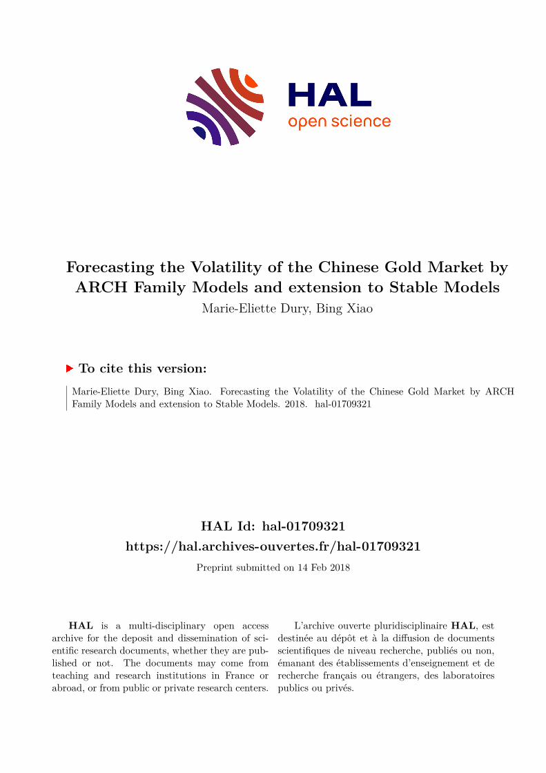
Our first step is to identify the mean equation for the returns. The autocorrelation and partial

autocorrelation function for the returns shows that autocorrelations and partial

autocorrelations up to the fifth lag are significant. We, therefore, propose using an

autoregressive moving average ARMA(1,1) mean equation to model volatility in the ARCH

models. The main criterion to choose our mean equation is the log likelihood. We noticed that

the AR model and the ARMA model provide the best quality of regression in terms of log

likelihood. The rest of the models obtained the same level of likelihood, of around 9862

against 9874 for AR(1) model and ARMA(1,1) model. For our mean equation, we chose

arbitrarily the ARMA(1,1) model for forecasting. The estimated ARMA(1,1) equation for the

mean is found to be a significant t-value for the coefficients. The residuals of the mean

equation indicate the absence of autocorrelation (Figures A7 and A8 in the Appendix).


Table 2: Mean equation estimated

AR(1) ARMA(1,1) AR(2) ARMA(2,2) AR(3) ARMA(3,3) AR(4) ARMA(4,4) AR(5) ARMA(5,5)

Log likelihood 9873.992 9874.152 9862.642 9862.172 9862.607 9862.825 9862.54 9862.525 9864.74 9864.856

Cons 0.000427

(0.031)

0.0004271

(0.033)

0.0004272

(0.044)

0.0004272

(0.046)

0.0004271

(0.040)

0.000427

(0.039)

0.0004272

(0.044)

0.0004272

(0.044)

0.0004275

(0.05)

0.000428

(0.055)

AR -0.0844319

(0.000)

-0.2212373

(0.070)

0.0152087

(0.178)

0.2311969

(0.758)

-0.0156923

(0.126)

0.2676657

(0.652)

0.0125475

(0.39)

-0.0764161

(0.931)

0.0388731

(0.000)

0.2769624

(0.323)

MA 0.1380424

(0.260)

-0.2151455

(0.775)

-0.2855026

(0.628)

0.0890251

(0.920)

-0.2387045

(0.404)

AR(6) ARMA(6,6) AR(7) ARMA(7,7) AR(8) ARMA(8,8) AR(9) ARMA(9,9) AR(10) ARMA(10,10)

Log likelihood 9862.868 9864.543 9862.59 9862.593 9862.27 9862.791 9863.369 9866.058 9862.366 9862.42

Cons 0.0004269

(0.037)

0.0004212

(0.016)

0.000427

(0.039)

0.0004269

(0.039)

0.0004267

(0.041)

0.0004272

(0.042)

0.0004275

(0.046)

0.0004274

(0.043)

0.0004274

(0.044)

0.0004272

(0.046)

AR -0.0192116

(0.067)

0.9011165

(0.000)

-0.0141387

(0.221)

0.0228311

(0.985)

-0.0020933

(0.854)

-0.7500928

(0.043)

0.0259658

(0.089)

-0.8711368

(0.000)

0.0079391

(0.494)

-0.3105028

(0.812)

MA -0.917304

(0.000)

-0.0370078

(0.975)

0.761945

(0.037)

0.8948036

(0.000)

0.3198109

(0.806)

p-values are given in parentheses


There is second-order dependence in the squared residuals of the mean equation and,

hence, the presence of conditional heteroscedasticity in the returns (Figures A7 and A8 in

the Appendix). Further, the ARCH-Lagrange Multiplier (LM) test confirms the presence

of ARCH effects and the need to model this conditional heteroscedasticity using the

ARCH family models (Table A3 in the Appendix).

The ARCH and GARCH models are easy to identify and estimate. But if « bad news » has a

more pronounced effect on volatility than « good news » of the same magnitude, the

symmetric specification such as ARCH or GARCH is not appropriate, because their

conditional variance is unaffected by the sign of the past period’s errors. It depends only on

squared errors. Before applying the asymmetric models, we can test the presence of

asymmetric effects. Engle and Ng (1993) propose various tests to detect the asymmetric

effects. After the GARCH regression, the squared residual is given by:

�� = � + ��I��

� + Y�� (22)

I�� = 1 where�� < 0, and 0 otherwise. If the dummy coefficient is significant and

positive, this suggests the presence of asymmetric effects. Then we can determine whether the

size of the negative shock also affects the impact on conditional variance by equation (23).

For the existence of a size effect, the coefficient must be negative and significant.

�� = �� + ��I�� + Y�� (23)

The positive sign bias test determines if the size of a positive shock impacts its conditional

variance, the regression is given by equation (24). For the size effect to be present, the

coefficient of I�� and I��\ �� must be significant.

�� = �� + ��I��\ �� + Y�� (24)

Tables 3 and 4 present the results of the models fitted to the data on returns with

Gaussian distribution and Student’s t distribution. The outputs on returns show that the

constant is statistically significant in the mean equation. The ARMA(1,1) term is also

statistically significant for all models except the ARCH(1). The variance equation illustrates

that all the terms are statistically significant at 1% level of significance which implies that the

volatility of risk is influenced by past square residual terms. It can be mentioned that the past

volatility of returns is significantly, influencing the current volatility. The EGARCH variance


equation also signifies that an asymmetric effect in volatility exists, which means that

positive shocks are affecting volatility differently to negative shocks.

Table 3 presents linear and non-linear GARCH parameter estimations for Chinese gold

market returns with Gaussian distribution. The coefficients of ARCH and GARCH models are

statistically significant, and GARCH (1,1) presents better likelihood at 10324. For the

GARCH model, the coefficient α+β =0.9762251 (0.1211033+0.8551218), indicates the

volatility shocks of SGE returns are persistent. The coefficients of IGARCH’s mean equation

are not significant. For the EGARCH model, the asymmetry parameter equals 0.2571219, it is

significantly positive, the coefficient of the ARCH term is positive at 10%, this indicates the

positive return shocks will have greater impacts on volatility. TARCH is created to capture

the negative movements of the volatility that usually is bigger than the positive movements.

In our case, the coefficient γ is 0.0277673 but significant at 1%.

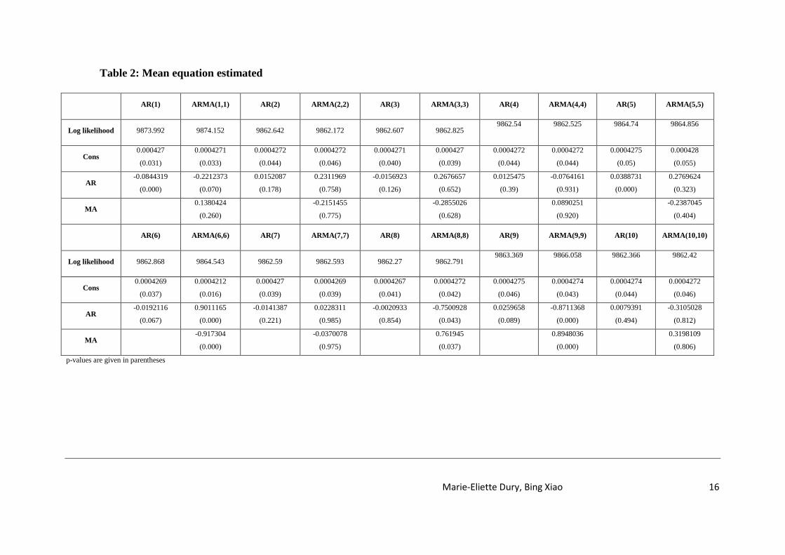
Table 4 presents the coefficients obtained with student’s distribution. The likelihood

parameter is greater than regression with Gaussian distribution, but the coefficients of mean

equation are not significant. The result of GARCH regression confirms the persistent

volatility shocks, α+β equals 0.9801919. The asymmetry parameter of the EGARCH model is

0.1760426 (significant at 1%), this result confirms the asymmetry return shocks. The

coefficient γ of TARCH model is significant by negative (-0.1333102 at 1%). This is an

unusual outcome; the result is contradictory in relation to our finding by using Gaussian

distribution. The negative coefficient means good news has a greater impact than bad news. In

a general way, the quality of the student’s distribution is not satisfactory, because of poor

significant coefficients of the mean equation. According to recent research, the financial

return time series with high kurtosis was better predicted by using the student’s distribution,

we will study the forecasting quality of the GARCH type models in the next section.


Table 3: Estimated coefficients for the ARCH models

ARCH(1) GARCH(1,1) IGARCH(1,1) EARCH(1,1) PARCH(1,1) TARCH(1,1) ARCHM(1) NARCH(1)

Cons_ 0.0004326

(0.019)

0.0003881

(0.011)

0.0003732

(0.016)

0.0004771

(0.007)

0.0003918

(0.013)

0.0004503

(0.010)

0.0022644

(0.000)

0.0003865

(0.047)

AR(L1) -0.5587494

(0.000)

-0.7068501

(0.005)

0.7353978

(0.284)

-0.9887848

(0.000)

-0.7230892

(0.002)

-0.7066202

(0.002)

-0.6623146

(0.000)

-0.5795511

(0.000)

MA(1) 0.4949706

(0.000)

0.6787811

(0.009)

-0.7264394

(0.297)

0.9958122

(0.000)

0.6942069

(0.004)

0.6761211

(0.005)

0.5985465

(0.000)

0.5111406

(0.000)

Variance equation

Cons_ 0.0001086

(0.000)

4.26e-06

(0.000)

3.04e-06

(0.000)

-0.334647

(0.000)

8.12e-07

(0.056)

3.98e-06

(0.000)

0.0001015

(0.000)

0.000108

(0.000)

ARCH(L1) 0.2366763

(0.000)

0.1211033

(0.000)

0.1420618

(0.000)

0.0112612

(0.087)

0.113781

(0.000)

0.107985

(0.000)

0.3098583

(0.000)

0.2381519

(0.000)

GARCH(L1) 0.8551218

(0.000)

0.8579351

(0.000)

0.9610151

(0.000)

0.8464523

(0.000)

0.8576062

(0.000)

Alpha 0.2571219

(0.000)

Power 2.359485

(0.000)

TARCH(L1) 0.0277673

(0.001)

ARCHM(σ²) -14.72094

(0.000)

NARCH (k) 0.0015396

(0.000)

likelihood 10011.67 10324.82 10317.69 10305.09 10326.75 10326.24 10026.58 10013.13

p-values are given in parentheses.


Table 4: Estimated coefficients for the ARCH models (Student distribution)

ARCH(1) GARCH(1,1) IGARCH(1,1) EGARCH(1,1) PARCH(1,1) TARCH(1,1) ARCHM(1) NARCH(1,1)

Cons_ 0.000677

(0.000)

0.0006195

(0.000)

0.0006202

(0.000)

0.0006417

(0.000)

0.0006812

(0.000)

0.0006775

(0.000)

0.0006564

(0.004)

0.0006234

(0.000)

AR(L1) -0.240092

(0.281)

-0.2711803

(0.343)

-0.2691433

(0.349)

-0.2181451

(0.404)

-0.2378837

(0.284)

-0.1672472

(0.487)

-0.2691172

(0.348)

-0.2240068

(0.335)

MA(1) 0.1850198

(0.417)

0.2158731

(0.457)

0.2131997

(0.464)

0.1571124

(0.552)

0.1824761

(0.421)

0.1151906

(0.637)

0.2138958

(0.462)

0.1712863

(0.470)

Variance equation

Cons_ 0.0001107

(0.000)

3.25e-06

(0.000)

2.54e-06

(0.000)

-0.1617319

(0.000)

0.0002089

(0.622)

0.0098154

(0.000)

3.24e-06

(0.000)

0.0001083

(0.000)

ARCH(L1) 0.275836

(0.000)

0.0957356

(0.000)

0.1114599

(0.000)

0.0205378

(0.065)

0.2775119

(0.000)

0.3175995

(0.000)

0.0955799

(0.000)

0.274595

(0.000)

GARCH(L1) 0.8844563

(0.000)

0.8885376

(0.000)

0.9806184

(0.000)

0.8846665

(0.000)

Alpha 0.1760426

(0.000)

Power 1.858312

(0.000)

TARCH(L1) -0.1333102

(0.004)

ARCHM(σ²) -0.3989969

(0.004)

NARCH (k) 0.002783

(0.015)

likelihood 10410.54 10543.41 10540.86 10550.85 10410.58 10411.7 10543.43 10413.6

df. 3.332802 4.416499 3.997225 4.271666 3.331899 3.328959 4.416377 3.34935



We test for the presence of asymmetric effects. The sign bias test yields the following results:

�� = 0.0001273 + 0.000305l��

� + Y��

p-value (0.000) (0.120)

�� = 0.0001579 − 0.000305l��

\ + Y��

p-value (0.000) (0.120)

A positive but not significant coefficient indicates the presence of leverage effects, implying

the positive and negative shocks may have a different effect on the conditional variance.

Estimating the negative and positive sign bias tests yields the following results:

�� = 0.0000751 − 0.0170669l��

� �� + Y��

p-value (0.000) (0.000)

�� = 0.0001372 + 0.0012538l��

\ �� + Y��

p-value (0.000) (0.352)

Significant coefficients on the negative sign bias-test imply that there are sign effects and size

effects. Positive and negative shocks do have a different effect on the conditional variance and

the negative effect on the variance depends on the size of the shocks.

4.1 In-Sample Statistical Performance

The following tables present the comparison of the in-sample statistical performance results

of the selected models. For the models with Gaussian distribution, they reveal that the

EGARCH has the lowest MAE and the lowest MAPE, the GARCH model and the IGARCH

model have the lowest RMSE at 3.53e-07. Based on the Student’s t distribution, the GARCH

and ARCHM model have the lowest MAE and the lowest MAPE. The IGARH model has the

lowest RMSE.

So, it can be said that, based on the outputs of in-sample statistical performance the GARCH

and EGARCH models are the best models for Gaussian distribution and the ARCHM model

is the best model for Student distribution. The ARCH, PARCH and NARCH models have the

worst MAE, MAPE and RMSE.


Table 5: In-sample statistical performance results (Gaussian distribution)

Model MAE MAPE RMSE

ARCH(1) 0.000193 8173.961 3.60e-07

GARCH(1,1) 0.0001914 5421.735 3.53e-07

EGARCH(1,1) 0.0001905 5156.383 3.55e-07

PARCH(1,1) 0.0001964 5437.983 3.55e-07

TARCH(1,1) 0.0001944 5345.467 3.55e-07

ARCHM(1) 0.0001925 8077.519 3.64e-07

IGARCH(1,1) 0.0002 5589.213 3.53e-07

NARCH(1) 0.0001932 8195.746 3.61e-07


Table 6: In-sample statistical performance results (Student distribution)

Model MAE MAPE RMSE

ARCH(1) 0.0001945 8490.761 3.56e-07

GARCH(1,1) 0.0001944 5385.746 3.57e-07

EGARCH(1,1) 0.0001917 5197.358 3.57e-07

PARCH(1,1) 0.0001945 8486.639 3.57e-07

TARCH(1,1) 0.0001981 8691.579 3.74e-07

ARCHM(1) 0.0001944 5383.354 3.57e-07

IGARCH(1,1) 0.000201 5798.238 3.55e-07

NARCH(1) 0.0001972 8520.639 3.57e-07

4.2 Out-Sample Statistical Performance

Having estimated the models, our next step is to assess their forecasts. We use the

models to make dynamic forecasts of volatility for the next 100 observations. For the

Gaussian distribution, the GARCH model has the lowest MAE at 0.000126 and the lowest

MAPE at 129.4682, the ARCH model has the lowest RMSE at 6.34e-08. Using Student’s t

distribution, the GARCH and ARCHM models have the lowest MAE, MAPE and RMSE.


Table 7: Out of sample statistical performance results (Gaussian distribution)

Model MAE MAPE RMSE

ARCH(1) 0.0001322 154.084 6.34e-08

GARCH(1,1) 0.000126 129.4682 6.69e-08

EGARCH(1,1) 0.0001314 142.6208 6.68e-08

PARCH(1,1) 0.0001266 131.3939 6.76e-08

TARCH(1,1) 0.0001276 133.4691 6.72e-08

ARCHM(1) 0.0001323 145.0933 6.37e-08

IGARCH(1,1) 0.0001279 137.4174 6.77e-08

NARCH(1) 0.0001329 153.1993 6.36e-08


Table 8: Out of sample statistical performance results (Student distribution)

Model MAE MAPE RMSE

ARCH(1) 0.0001359 158.3068 6.37e-08

GARCH(1,1) 0.0001254 127.5605 6.67e-08

EGARCH(1,1) 0.0001284 133.2779 6.59e-08

PARCH(1,1) 0.0001358 157.9436 6.35e-08

TARCH(1,1) 0.0001345 154.4988 6.32e-08

ARCHM(1) 0.0001254 127.5211 6.07e-08

IGARCH(1,1) 0.0001348 135.4212 7.03e-08

NARCH(1) 0.0001351 156.5947 6.41e-08

5. Conclusion

This study has implications for investors who wish to price, hedge and speculate in the

Chinese gold market. Gold is an underlying asset in which volatility is an important factor

when pricing options. Secondly, the investor may use the Gold futures contracts to hedge their

underlying Gold position. Forecasting volatility may be important for investors for adjusting

their hedging strategies. In a general way, understanding how information (bad news and

good news) impacts on return volatility improves the performance of portfolio management.

For example, this knowledge allows the investors to have a better portfolio selection in asset

pricing and allows them a more efficient risk management. In addition, the Chinese gold

market offers an opportunity for international diversification.


Our study has attempted to model gold prices at the Shanghai Gold Exchange (SGE) return

and assess the forecasting ability of the ARCH family of models. We have used historical

volatility for modeling purposes through the ARCH family of models and made dynamic

forecasts of future volatility. The analysis covers from October 30, 2002 to December 7, 2015

and from December 8, 2015 to May 6, 2016 as in-sample and out-of-sample sets respectively.

For the Gaussian distribution, the results of the in-sample statistical performance show that

the GARCH and EARCH models are selected as the best performing models for the returns.

According to the outcomes of MAE and MAPT, the EGARCH model is better than the

GARCH model in explaining the return (modeling the volatility), furthermore, using t-student

distribution, the EGARCH model gets the best MAPE estimation of all models. This finding

confirms our asymmetric effect analysis. Outcomes of the out-of-sample statistical

performance demonstrate that the GARCH is considered to be the best model. Based on

Student’s t distribution, the GARCH and the ARCHM models are the best models for in and

out-of-samples. This result confirms the power of the GARCH model in prediction volatility

by using t-student distribution. At the same time, the ARCHM model shows good predicting

capacity, in our study, volatility shocks appear persistent for the Gold return series as the sum

of the coefficients α and β is close to unity for all estimated models. According to Engle and

Bollerslev (1986, 1987), including conditional variance in the conditional mean equation is

more appropriate for financial time series when the expected return on an asset is related to

the expected asset risk. At the same time, the ARCHM model shows good predicting

capacity, this result corroborates the finding of Zou, Rose and Pinflod (2007), in which they

conclude the EGARCH and ARCHM models outperform all other models in capturing the

dynamic return volatility for Australian Three-Year T-Bond futures contracts. Two other facts

have caught our attention: firstly, the specification of mean equation by using t-student

distribution is not satisfactory; this study demonstrates that it is necessary to improve the

quality of the mean equation estimates. Secondly, the quality of PARCH regression is not

satisfactory, according to the PARCH model, the power term allows the capture volatility by

changing the influence of the extreme value. But, according to new literature review, when

the return is non-normally distributed, the use of a power transformation is not appropriate.

We think using stable process distribution would be a solution to this issue, the extension to

Stable Models opens up new paths for this research, this approach allows us to represent high


volatility. Next step is the simulation of the model for which we have to develop the computer

programming.

Bibliography

Awartani M.A., Corradi V., Predicting the Volatility of the S&P500 Stock Index via GARCH

Models: The Role of Asymmetries, International Journal of Forecasting, (2005) 21, (1), 167-

183.

Bachelier L., Théorie de la speculation, Annales scientifiques de l’Ecole Normale Supérieure,

3ème série, t.17, Paris (1900), Gauthier-Villars, p.21-86 (reprint 1995)

Benassi A., Cohen S., Istas J., Identification and properties of real Harmonizable Fractional

Lévy Motions, Bernoulli (2002) vol.8, number 1, 97-115

Benassi A., Jaffard S., Roux D., Elliptic Gaussian Random Processes, Fractals: Theory and

Applications in Engineering, (1999) Springer-Verlag, p.33-45

Bollerslev T., Generalized autoregressive conditional heteroscedasticity. Journal of

Econometrics, (1986), 31, 307–327.

Bollerslev T., A Conditionally Heteroskedastic Time Series Model for Speculative Prices and

Rates of Return, The Review of Economics and Statistics, (Aug., 1987) Vol. 69, (3) 542-547.

Bracker K., Smith K. L., Detecting and modeling volatility in the copper futures market.

Journal of Futures Markets, (1999), 19(1), 79–100.

Cambanis S., Maejima M., Two classes of self-similar stable processes with stationary

increments, Stochastic Processes and their Applications, (1989) v.32, 305-329

Carvalho A. F., da Costa J. S., Lopes J. A., A systematic modeling strategy for futures

markets volatility. Applied Financial Economics, (2006), 16, 819–833.

Ciner C., On the long run relationship between gold and silver: a note. Global Finance Journal

(2001) 12, 257-278.

Dury M-E., Estimation du paramètre de Hurst de processus stables autosimilaires à

accroissements stationnaires, C.R.Acad.Sci.Paris, Série I 333 (2001) 45-48


Ederington H. L., Guan W., Forecasting volatility. Journal of Futures Markets. (2005), 25(5),

465-490.

Engle R. F., Autoregressive conditional heteroscedasticity with estimates of the variance of

United Kingdom inflation. Econometrica, (1982), 50, 987–1007.

Engle R.F., Bollerslev T., Modelling the Persistence of Conditional Variance, Econometric

Review, (1986) 5 (1), 1-50.

Grek A., Forecasting accuracy for ARCH models and GARCH(1,1) family – Which model

does best capture the volatility of the Swedish stock market ? Spring 2014, Orebro University

Goyal A., Predictability of Stock Return Volatility from GARCH Models (2000)

http://www.hec.unil.ch/agoyal/docs/Garch.pdf (Accessed January 2016).

Hoang T, Lean H.H., Wong W.K., Is Gold Good for Portfolio Diversification? A Stochastic

Dominance Analysis of the Paris Stock Exchange, International Review of Financial Analysis

(2015), 42: 98-108.

Köksal B., A Comparison of Conditional Volatility Estimators for the ISE National 100 Index

Returns. Journal of Economic and Social Research, (2009), 11(2), page 1-28.

Marcucci, J., Forecasting Stock Market Volatility with Regime-Switching GARCH Models

(2005) Department of Economics, University of California. San Diego

Mandelbrot B.B., Van Ness J.W., Fractional Brownian Motion, Fractional Noises and

Applications, SIAM Review (1968), v.10, n°4, p.422-437

Mitchell J. D., Ong L.L., Seasonalities in China’s Stock Markets: Cultural or Structural? IMF

Working Paper, January 2006, Monetary and Financial Systems Department, University of

Michigan. https://www.imf.org/external/pubs/ft/wp/2006/wp0604.pdf (Accessed July 2016).

Mookerjee R., Yu Q., An empirical analysis of the equity markets in China, Review of

Financial Economics (1999), 8, (1), 41-60.

Nelson D. B., Conditional heteroscedasticity in asset returns: A new approach, Econometrica,

(1991), 59, 347–370.


Peltier R-F., Lévy Véhel J., Multifractional Brownian Motion: Definition and Preliminary

Results, Rapport de recherché INRIA 2645 (1995)

Poon S.-H., & Granger C. W. J., Forecasting volatility in financial markets: A review. Journal

of Economic Literature, (2003), 41, 478–539.

Ramasamy R., Munisamy S. Predictive Accuracy of GARCH, GJR and EGARCH Models

Select Exchange Rates Application, Global Journal of Management and Business Research,

(2012), 12(15) 81.

Rosovskii L.V., Probabilities of Large Deviations for Sums of Independent Random Variables

with a common Distribution Function from the Domain of Attraction of an Asymmetric

Stable Law, Theory Prob. Appli. 42 (1995) n°3, 454-482

Sadorsky P., Modeling and forecasting petroleum futures volatility. Energy Economics,

(2006), 28, 467–488.

Samorodnitsky G., Taqqu M.S., Stable Non-Gaussian Random Processes: Stochastic models

with infinite Variance, Chapman&Hall (1994)

Sjaastad L.A., Scacciavillani F., The price of gold and the exchange rate. Journal Int. Money

Finance (1996) 15, 879-897.

Smith G., London Gold Prices and Stock Prices in Europe and Japan, (2002) World Gold

Council, London.

Solt M., Swanson P., On the efficiency of the markets for gold and silver. Journal of Business

(1981) 54, 453-478.

Taqqu Murad.S., Pipiras V., Stable Non-Gaussian Self-Similar Processes with Stationary

increments, Springer Briefs in Probability and Mathematical Statistics (2017)

Tareena Musaddiq, Modeling and Forecasting the Volatility of Oil Futures Using the ARCH

Family Models, The Lahore Journal of Business, 1:1 (Summer 2012): pp. 79–108.

Taylor S., Modeling financial time series (1986) Chichester, UK: Wiley

Tully E., Lucey B.M., A power GARCH examination of the gold market, Research in

International Business and Finance, (2007) 21, 316-325.


Zahangir Alam, Noman Siddikee and Masukujjaman, Forecasting Volatility of Stock Indices

with ARCH Model, International Journal of Financial Research, (2013) Vol. 4, No. 2

Zakoïan J.-M., Threshold heteroscedastic models. Journal of Economic Dynamics and

Control, (1994), 18, 931–955.

Zou L., Rose L., Pinfold J., Asymmetric Information impacts: Evidence from the Australian

Treasury-Bond Futures Markets, Pacific Economic Review, (2007) 12:5


Appendix:

Tables

Table A1: Summary statistics for SGE Index

Obs Mean Std. Dev. Skewness Kurtosis

SGE Index 3279 211.5135 79.11776 0.11876799 -1.04121692

Table A2: Dickey-Fuller test for SGE index

Test statistic 1% critical value 5% critical value 10% critical value p-value for Z(t)

-1.544 -3.430 -2.860 -2.570 0.5119

Table A3: Phillips-Perron test for SGE index

Test statistic 1% critical value 5% critical value 10% critical value

Z(rho) -2.785 -20.700 -14.100 -11.300

Z(t) -1.494 -3.430 -2.860 -2.570

MacKinnon approximate p-value for Z(t) = 0.5364

Table A4: Dickey-Fuller test for returns

Test statistic 1% critical value 5% critical value 10% critical value p-value for Z(t)

-62.283 -3.430 -2.860 -2.570 0.0000

Table A5: Phillips-Perron test for returns

Test statistic 1% critical value 5% critical value 10% critical value

Z(rho) -3595.529 -20.700 -14.100 -11.300

Z(t) -62.222 -3.430 -2.860 -2.570

MacKinnon approximate p-value for Z(t) = 0.0000

Table A6: LM test for autoregressive conditional heteroscedasticity

Lags(p) Chi² Df Prob. > Chi²

1 241.180 1 0.0000

H0: No ARCH effects vs. ARCH(p) disturbance


-0.5

00.

000.

501.

00A

utoc

orre

latio

ns o

f clo

sepr

ice

s

0 10 20 30 40Lag

Bartlett's formula for MA(q) 95% confidence bands

0.00

0.20

0.40

0.60

0.80

1.00

Par

tial a

utoc

orre

latio

ns o

f clo

sepr

ices

0 10 20 30 40Lag

95% Confidence bands [se = 1/sqrt(n)]

-0.1

00.

000.

100.

200.

30A

utoc

orre

latio

ns o

f Ren

t2

0 10 20 30 40Lag


-0.1

00.

000.

100.

200.

30P

artia

l aut

oco

rre

latio

ns o

f Ren

t2

0 10 20 30 40Lag


-0.1

0-0

.05

0.00

0.05

Aut

oco

rrel

atio

ns o

f Ren

t

0 10 20 30 40Lag


-0.1

0-0

.05

0.00

0.05

Par

tial a

utoc

orre

latio

ns o

f Ren

t

0 10 20 30 40Lag


Figures

Figure A1: AC of SGE index Figure A2: PAC of SGE index

Figure A3: AC of squared returns Figure A4: PAC of squared returns

Figure A5: AC of Returns Figure A6: PAC of Returns


-0.0

4-0

.02

0.00

0.02

0.04

Aut

oco

rrel

atio

ns o

f err

_mea

n_eq

u

0 10 20 30 40Lag


-0.0

4-0

.02

0.00

0.02

0.04

Par

tial a

utoc

orre

latio

ns o

f err

_mea

n_e

qu

0 10 20 30 40Lag


-0.1

00.

000.

100.

200.

30A

utoc

orre

latio

ns o

f err

_m

ean_

equ2

0 10 20 30 40Lag


-0.1

00.

000.

100.

200.

30P

artia

l au

toco

rrel

atio

ns o

f err

_me

an_e

qu2

0 10 20 30 40Lag


Figure A7: AC of res. mean equation Figure A8: PAC of res. mean equation

Figure A9: AC of res.² mean equation Figure A10: PAC of res.² mean

equation

Documents

Forecasting the Volatility of the Chinese Gold Market by