Forecasting the Return Distribution Using High-Frequency

Volatility Measures

Jian Hua and Sebastiano Manzan

Department of Economics & Finance

Zicklin School of Business, Baruch College, CUNY

Abstract

The aim of this paper is to forecast (out-of-sample) the distribution of financialreturns based on realized volatility measures constructed from high-frequencyreturns. We adopt a semi-parametric model for the distribution by assumingthat the return quantiles depend on the realized measures and evaluate the dis-tribution, quantile and interval forecasts of the quantile model in comparison toa benchmark GARCH model. The results suggest that the model outperformsan asymmetric GARCH specification when applied to the S&P 500 futures re-turns, in particular on the right tail of the distribution. However, the modelprovides similar accuracy to a GARCH(1,1) model when the 30-year Treasurybond futures return is considered.

JEL Classification: C14; C22; C53Keywords: Realized Volatility; Quantile Regression; Density Forecast; Value-at-Risk

Corresponding author: Sebastiano Manzan, Department of Economics and Finance, Baruch College, 55

Lexington Avenue, New York, NY 10010; phone: 646-312-3408, email: sebastiano.manzan@baruch.cuny.edu

1 Introduction

Until recently, the predominant approach in modeling the conditional distribution of returns was

represented by the ARCH-GARCH model proposed by Engle (1982) and Bollerslev (1986) and

followed by a myriad of sophisticated refinements to the baseline model. The GARCH model

introduces time variation in the conditional distribution largely through the conditional variance,

and has been successful in explaining several empirical features of asset returns, such as fat tails

and the slowly decaying autocorrelation in squared returns. While the GARCH model assumes a

parametric form for the latent variance of returns, the recent availability of high-frequency data

has sparked a growing literature of volatility estimators that do not require researchers to specify

a model. The so-called realized volatility literature (see Andersen and Bollerslev, 1998, Andersen

et al., 2001a and 2001b among others) uses high-frequency data to proxy for the volatility of lower

frequency returns, for instance, summing intra-day squared returns to estimate the daily variance.

In this way, the latent variance process is observable and measured by realized volatility which

facilitates the task of modeling and forecasting using time series models. Several recent papers

incorporate these measures within a parametric volatility model for the dynamics of daily returns

(see Shephard and Sheppard, 2010, Brownlees and Gallo, 2010, Maheu and McCurdy, 2011, and

Hansen et al., 2011).

In this paper we propose to relate the realized volatility measures and returns by assuming that

these measures represent the driving force for the variation of the quantiles of the cumulative

multi-period return distribution. In particular, the flexibility of the quantile regression model (see

Koenker and Bassett, 1978) allows to consider several specifications that include smoothed versions

of the realized volatility measures, the return standardized by realized volatility and nonlinear

transformations of the return that are considered to account for the leverage effect. The fact that

the parameters of the quantile regression model are specific to each quantile level allows the variables

to have heterogeneous effects in different parts of the return distribution. In addition, the quantile

model does not require to specify a distribution for the error as it is instead the case for GARCH

models or for models based on realized volatility measures. Hence, the flexibility in choosing the

most appropriate explanatory variables, the adaptability of the effect of these variables at each

quantile level, and the distribution-free character of the method are the three characteristics that

distinguish our approach from the models recently proposed in the literature that related realized

volatility and returns. The application of quantile regression to modeling and forecasting financial

returns has experienced a recent surge of interest due to the emergence of risk management and its

focus on forecasting the return quantiles (see Engle and Manganelli, 2004, Xiao and Koenker, 2009,

Zikes, 2010, and Gaglianone et al., 2011). Another aspect that distinguishes our paper is the method

adopted to evaluate the performance of quantile and distribution forecasts. A common loss function

used in the comparison of density forecasts is the logarithmic score rule, which rewards forecasts that

have higher density at the realization of the variable being forecast (see, among others, Bao et al.,

2007, Amisano and Giacomini, 2007, and Maheu and McCurdy, 2011, and Shephard and Sheppard,

2010 for two applications in the realized volatility literature). Although this is certainly a relevant

criterion to consider, it does not reward forecasts that assign high probabilities to values close to

2

the realization in addition to the fact that it cannot be easily adapted to evaluate specific areas of

the distribution, for instance the left or right tail. Gneiting and Raftery (2007) and Gneiting and

Ranjan (2011) discuss alternative rules that overcome these problems, and we consider several of

these rules to evaluate different characteristics of the return distribution. In particular, we use the

Quantile Score rule represented by the tick loss function which is targeted to quantile forecasts, such

as VaR (e.g. Clements et al., 2008). Instead of focusing on few quantiles of interests, we examine

several of them that span the complete return distribution which allows to evaluate the forecast

performance of the competing models in different areas of the distribution. Furthermore, we also

consider a weighted version of the Quantile Score rule that evaluates specific areas of the forecast

distribution, for instance the left and right tail or the center of the distribution, and a scoring rule

that evaluates interval forecasts at the 50 and 90% level.

In the empirical application we consider the S&P 500 index futures (SP) and the 30-year Treasury

bond futures (US) and forecast out-of-sample the cumulative return at the 1, 2, and 5-day horizons.

We evaluate and compare the forecasts from the realized volatility quantile model to those of a

benchmark GARCH model represented by the GJR specification (Glosten et al., 1993) for the

SP returns and the simple GARCH(1,1) for the US returns. We consider several high-frequency

measures of volatility that have been proposed in the literature, including several adjustments that

account for the presence of microstructure noise and jumps. The results for the SP returns indicate

that the distribution forecasts at the 1-day horizon from the realized volatility models outperform

those from the GJR model, with the improved performance mostly deriving from the better ability to

forecast the right tail of the return distribution. Only the specifications that include an asymmetric

effect are able to beat GJR in modeling the left tail, and significantly so for quantile levels between 20

and 30%. Furthermore, the comparison suggests that the realized measures of volatility considered

deliver very similar results, thus indicating that filtering out the effect of jumps and micro-structure

noise does not improve the (out-of-sample) forecasting ability in any part of the return distribution.

In addition, we also consider some quantile specifications that use absolute daily returns (and their

transformations), instead of the realized measures, and the evidence indicates that their forecasts

do not outperform those from the GJR benchmark. This result indicates that the flexibility of the

quantile model combined with the (absolute) returns produces forecasts that have similar accuracy

relative to GARCH models, although it does not require to assume a parametric specification. In

addition, the realized volatility measures provide valuable information that can be used to improve

the accuracy of forecasts relative to (quantile or GARCH) models that only use returns. However,

the evidence for the US bond return shows that the realized volatility quantile models provide

similarly accurate forecasts relative to those of the benchmark GARCH(1,1) model at all horizons.

In this case thus the realized volatility measures do not provide additional forecasting power for the

return distribution compared to what is already embedded in daily returns, contrary to the results

for the equity index returns.

The paper is organized in this manner. Section (2) describes the realized measures of volatility

that are considered in this paper, while Section (3) introduces the GARCH specifications and the

semi-parametric model that we propose to incorporate the realized measures in modeling return

3

quantiles. Section (4) describes the forecast evaluation methods and Section (5) reports the results

of the empirical application. Finally, Section (7) concludes.

2 Realized volatility estimators

The availability of high-frequency data has sparked the development of methods to estimate the

(latent) volatility of financial returns that do not require the specification of a model. The most

well-known quantity is realized volatility which is obtained by summing intra-day squared returns

and can be used to proxy for integrated volatility (see Andersen and Bollerslev, 1998, Barndorff-

Nielsen and Shephard, 2002a, 2002b, Meddahi, 2002). In this Section, we present several realized

volatility measures that are later used in our empirical application.

Denote the intra-day return in day t by rt,i = ln(Pti) − ln(Pti−1), where i = 1, 2, . . . ,m indicates

the intra-day interval and Pti the asset price in interval i of day t. The realized volatility estimator

in day t, denoted by RVt, represents a model-free estimator of the daily quadratic variation at

sampling frequency m and is given by

RVt =m∑i=1

r2t,i. (1)

The asymptotic distribution of RVt has been studied by Andersen and Bollerslev (1998), Andersen

et al. (2001b), Andersen et al. (2003), and Barndorff-Nielsen and Shephard (2002a), among others.

An important role in the construction of the measure is played by the selection of the sampling

frequency m which is complicated by several market microstructure issues (see, e.g. Ait-Sahalia

et al., 2005a, Ait-Sahalia et al., 2005b, Bandi and Russell, 2008, Hansen and Lunde, 2006b, and

Barndorff-Nielsen et al., 2008, among others). In our empirical application, we use a five-minute

sampling frequency, which has been shown in the literature to strike a reasonable balance between

the desire for as finely sampled observations as possible and robustness to market microstructure

contaminations.

Despite the careful selection of sampling frequency, market-microstructure dynamics could still

cause RVt to be a biased and inconsistent estimator of volatility. Thus, we also consider estimators

with adjustments that reduce market microstructure frictions present in high-frequency returns.

We adopt a kernel-based estimator of realized volatility suggested by Hansen and Lunde (2006b),

which employs Bartlett weights,

RV (q)t =m∑i=1

r2t,i + 2q∑

w=1

(1− w

q + 1

)m−w∑i=1

rt,irt,i+w, (2)

where rt,i is defined as above and(1− w

q+1

)represents the weight that follows a Bartlett scheme.

This estimator utilizes higher-order auto-covariances to eliminate the bias of RVt, and is also guar-

anteed to be non-negative. The asymptotic properties of the estimator are discussed by Barndorff-

Nielsen et al. (2008).

4

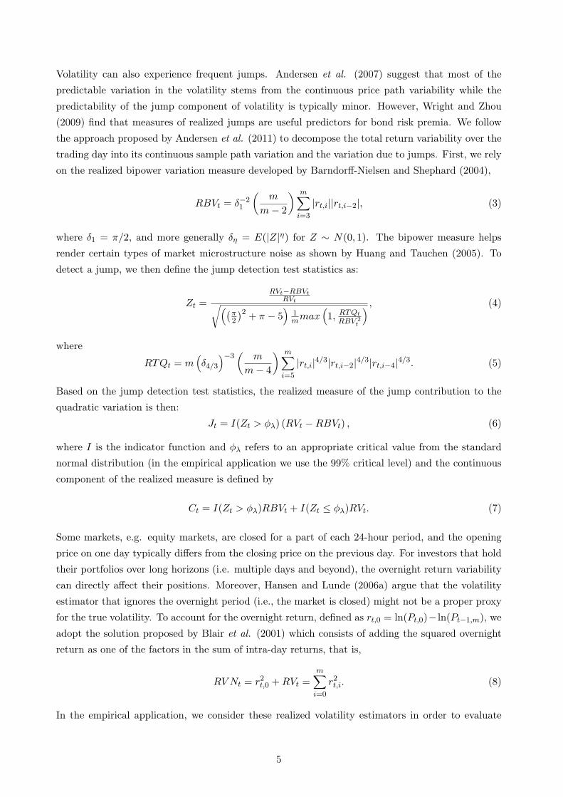
Volatility can also experience frequent jumps. Andersen et al. (2007) suggest that most of the

predictable variation in the volatility stems from the continuous price path variability while the

predictability of the jump component of volatility is typically minor. However, Wright and Zhou

(2009) find that measures of realized jumps are useful predictors for bond risk premia. We follow

the approach proposed by Andersen et al. (2011) to decompose the total return variability over the

trading day into its continuous sample path variation and the variation due to jumps. First, we rely

on the realized bipower variation measure developed by Barndorff-Nielsen and Shephard (2004),

RBVt = δ−21

(m

m− 2

) m∑i=3

|rt,i||rt,i−2|, (3)

where δ1 = π/2, and more generally δη = E(|Z|η) for Z ∼ N(0, 1). The bipower measure helps

render certain types of market microstructure noise as shown by Huang and Tauchen (2005). To

detect a jump, we then define the jump detection test statistics as:

Zt =RVt−RBVt

RVt√((π2

)2 + π − 5)

1mmax

(1, RTQt

RBV 2t

) , (4)

where

RTQt = m(δ4/3

)−3(

m

m− 4

) m∑i=5

|rt,i|4/3|rt,i−2|4/3|rt,i−4|4/3. (5)

Based on the jump detection test statistics, the realized measure of the jump contribution to the

quadratic variation is then:

Jt = I(Zt > φλ) (RVt −RBVt) , (6)

where I is the indicator function and φλ refers to an appropriate critical value from the standard

normal distribution (in the empirical application we use the 99% critical level) and the continuous

component of the realized measure is defined by

Ct = I(Zt > φλ)RBVt + I(Zt ≤ φλ)RVt. (7)

Some markets, e.g. equity markets, are closed for a part of each 24-hour period, and the opening

price on one day typically differs from the closing price on the previous day. For investors that hold

their portfolios over long horizons (i.e. multiple days and beyond), the overnight return variability

can directly affect their positions. Moreover, Hansen and Lunde (2006a) argue that the volatility

estimator that ignores the overnight period (i.e., the market is closed) might not be a proper proxy

for the true volatility. To account for the overnight return, defined as rt,0 = ln(Pt,0)− ln(Pt−1,m), we

adopt the solution proposed by Blair et al. (2001) which consists of adding the squared overnight

return as one of the factors in the sum of intra-day returns, that is,

RV Nt = r2t,0 +RVt =m∑i=0

r2t,i. (8)

In the empirical application, we consider these realized volatility estimators in order to evaluate

5

their informational content to forecast the distribution of financial returns.

3 Forecasting models

As discussed earlier, the aim of the analysis is to evaluate the relevance of incorporating high-

frequency measures of volatility to forecast (out-of-sample) the return distribution as opposed to

adopting a GARCH-type time-series model. In this Section, we first introduce the GARCH specifi-

cations from which we select the benchmark for the forecast comparison, followed by a discussion of

the approach we propose to incorporate high-frequency volatility measures in the return distribution.

3.1 GARCH models

Hansen and Lunde (2005) provide an extensive comparison of the (out-of-sample) volatility forecasts

accuracy of 330 GARCH-type specifications. Their results show that the simple GARCH(1,1) model

of Bollerslev (1986) is hardly outperformed by more sophisticated specifications when forecasting

daily exchange rate volatility, although it is beaten by models that include a leverage effect when

forecasting stock returns. Based on these results, we decided to consider in our out-of-sample

comparison a small set of models which comprise the simple GARCH(1,1) and two of the most

frequently used specifications with leverage effects, the EGARCH of Nelson (1991) and the GJR-

GARCH model of Glosten et al. (1993).

We denote the close-to-close return on day t+ 1 by rt+1 = ln(Pt+1)− ln(Pt), where Pt indicates the

closing price of the asset in day t. We assume that the returns follow a time-varying location-scale

model given by rt+1 = µ + εt+1, where µ is a constant and εt+1 = σt+1ηt+1, with σt+1 denoting

the conditional standard deviation in day t+ 1 and ηt+1 is an i.i.d. error term with mean zero and

variance one. To fully specify the distribution of the return rt+1 we need to introduce assumptions

on both the dynamics of the conditional variance and the distribution of the error term ηt+1. As

concerns the conditional variance, we consider three specifications:

1. GARCH(1,1): σ2t+1 = ω + αε2t + βσ2

t

2. GJR-GARCH(1,1): σ2t+1 = ω + αε2t + γε2t I(εt < 0) + βσ2

t

3. EGARCH(1,1): ln(σ2t+1

)= ω + α(|ηt| − E|ηt|) + γηt + β ln

(σ2t

)where ω, α, β and γ are parameters. The characteristic of the GJR and EGARCH specifications

is to allow the current shock to have an asymmetric effect on volatility. The empirical evidence

suggests that volatility increases more following negative surprises compared to positive ones of

the same magnitude. The second hypothesis concerns the distribution of the error term ηt+1.

In this case, we consider the parametric assumptions that ηt+1 is distributed according to the

standard normal distribution, or that it follows the Student tk distribution, where k indicates

the degrees of freedom. In both cases we estimate the parameters by Maximum Likelihood. In

addition to these two parametric assumptions, we also consider a non-parametric approach which

consists of resampling from the Empirical Distribution Function (EDF) of the standardized residuals.

The advantage of using this approach is that we abstract from assuming a parametric form, and

6

instead let the data indicate the shape of the distribution that might, possibly, be characterized

by (unconditional) skewness and excess kurtosis (see Bali et al., 2008, for an approach that allows

for time-varying skewness and kurtosis). The combination of a GARCH-type specification for the

conditional variance and errors resampled from the EDF is typically referred to as Filtered Historical

Simulation (FHS). Barone-Adesi et al. (2011) provide a recent application of FHS to option pricing.

In addition to the one-day ahead return distribution, we are also interested in forecasting the

cumulative h-day ahead return defined as rht+h = ln(Pt+h)− ln(Pt). The conditional variance of the

h-day cumulative return for the GARCH(1,1) and GJR models is obtained by σ2t+h =

∑hj=1 σ

2t+j ,

which is then combined with the two parametric assumptions on the error distribution to obtain the

h-day ahead forecast of the cumulative return CDF, denoted by Ft+h(·), and the predictive quantile

at level τ by F−1t+h(τ). Instead, for the FHS approach the distribution of rht+h is approximated

by simulating a large number B of return paths in two steps: (1) estimate the GARCH(1,1),

GJR, or EGARCH specification by quasi-ML and obtain the standardized residuals, and (2) iterate

forward the model using the estimated parameters and the resampled standardized residuals as

innovations. This provides B return paths based on the one-step ahead model discussed above and

the distribution of the cumulative return can be approximated by the EDF of rht+h,b =∑hj=1 rt+j,b,

where b = 1, · · · , B.

3.2 Realized volatility models

As discussed earlier, realized volatility measures represent model-free estimates of volatility, in the

sense that they do not rely on the assumption of a parametric model, for instance a GARCH

model. Andersen et al. (2001a, 2001b, 2003), among others, propose time series models for realized

volatility measures (or a log-transformation) in order to explain their in-sample dynamics as well as

to forecast and evaluate the volatility process. Recently, several papers (e.g. Engle and Gallo, 2006,

Bollerslev et al., 2009, Shephard and Sheppard, 2010, Brownlees and Gallo, 2010, and Maheu and

McCurdy, 2011, and Hansen et al., 2011) depart from the univariate analysis of realized volatility

and propose joint models of the dynamics of returns and realized volatility measures.

In this paper, we use the realized measures to explain the time variation of the conditional quantiles

of returns which can be illustrated based on the location-scale model rt+1 = µ+ σt+1ηt+1 discussed

in the previous Section. The quantile at level τ for this model, conditional on information available

at time t, Ft, is given by qt+1(τ |Ft) = µ+σt+1qη(τ), where qη(τ) represents the τ -th quantile of the

error term distribution. Since we assume that the conditional mean µ and the quantiles of the error

qη(τ) are constants, the return quantile varies over time only through changes in the conditional

standard deviation of the process. We then introduce the hypothesis that the variation in the

conditional variance σ2t+1 is equal to the expected realized volatility measure in day t+ 1, denoted

by Et(RMt+1), where by RMt+1 we denote any of the unbiased estimators of quadratic variation that

were discussed in Section (2). We can assume that the variation in the expected realized measure

is a function of a set of variables observable at time t, Xt, which might include past values of the

measure and past returns, among others. Based on these assumptions, the conditional variance of

returns becomes σ2t+1 = (δ0 + X ′tδ1)2, where δ0 and δ1 are parameters and where we assume that

7

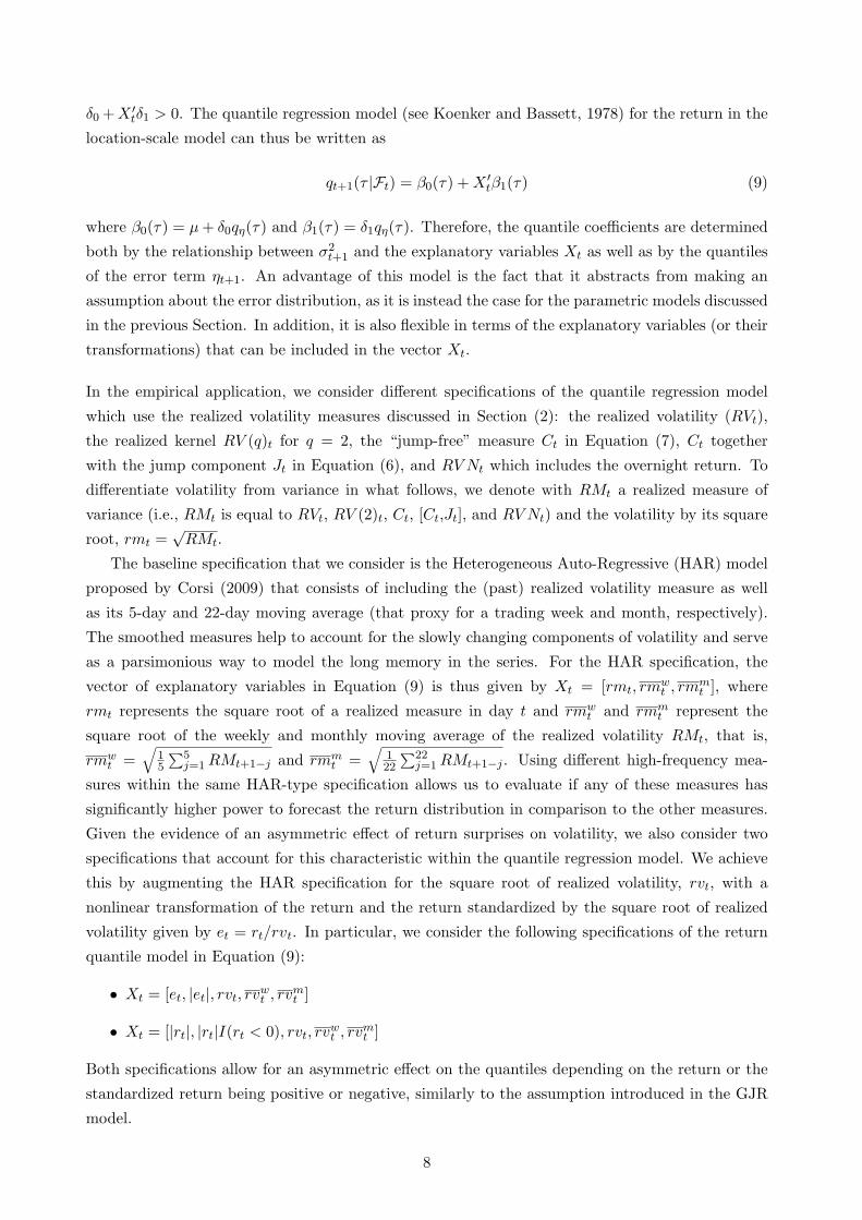
δ0 +X ′tδ1 > 0. The quantile regression model (see Koenker and Bassett, 1978) for the return in the

location-scale model can thus be written as

qt+1(τ |Ft) = β0(τ) +X ′tβ1(τ) (9)

where β0(τ) = µ+ δ0qη(τ) and β1(τ) = δ1qη(τ). Therefore, the quantile coefficients are determined

both by the relationship between σ2t+1 and the explanatory variables Xt as well as by the quantiles

of the error term ηt+1. An advantage of this model is the fact that it abstracts from making an

assumption about the error distribution, as it is instead the case for the parametric models discussed

in the previous Section. In addition, it is also flexible in terms of the explanatory variables (or their

transformations) that can be included in the vector Xt.

In the empirical application, we consider different specifications of the quantile regression model

which use the realized volatility measures discussed in Section (2): the realized volatility (RVt),

the realized kernel RV (q)t for q = 2, the “jump-free” measure Ct in Equation (7), Ct together

with the jump component Jt in Equation (6), and RV Nt which includes the overnight return. To

differentiate volatility from variance in what follows, we denote with RMt a realized measure of

variance (i.e., RMt is equal to RVt, RV (2)t, Ct, [Ct,Jt], and RV Nt) and the volatility by its square

root, rmt =√RMt.

The baseline specification that we consider is the Heterogeneous Auto-Regressive (HAR) model

proposed by Corsi (2009) that consists of including the (past) realized volatility measure as well

as its 5-day and 22-day moving average (that proxy for a trading week and month, respectively).

The smoothed measures help to account for the slowly changing components of volatility and serve

as a parsimonious way to model the long memory in the series. For the HAR specification, the

vector of explanatory variables in Equation (9) is thus given by Xt = [rmt, rmwt , rm

mt ], where

rmt represents the square root of a realized measure in day t and rmwt and rmm

t represent the

square root of the weekly and monthly moving average of the realized volatility RMt, that is,

rmwt =

√15

∑5j=1RMt+1−j and rmm

t =√

122

∑22j=1RMt+1−j . Using different high-frequency mea-

sures within the same HAR-type specification allows us to evaluate if any of these measures has

significantly higher power to forecast the return distribution in comparison to the other measures.

Given the evidence of an asymmetric effect of return surprises on volatility, we also consider two

specifications that account for this characteristic within the quantile regression model. We achieve

this by augmenting the HAR specification for the square root of realized volatility, rvt, with a

nonlinear transformation of the return and the return standardized by the square root of realized

volatility given by et = rt/rvt. In particular, we consider the following specifications of the return

quantile model in Equation (9):

• Xt = [et, |et|, rvt, rvwt , rvmt ]

• Xt = [|rt|, |rt|I(rt < 0), rvt, rvwt , rvmt ]

Both specifications allow for an asymmetric effect on the quantiles depending on the return or the

standardized return being positive or negative, similarly to the assumption introduced in the GJR

model.

8

The ultimate goal of the paper is to evaluate whether the realized volatility models provide more

accurate forecasts of the return quantiles and distribution relative to a GARCH-type time series

model. In order to disentangle the contribution to the forecast performance that derives from the

realized volatility measures as opposed to the contribution of the semi-parametric character of the

quantile regression model, we also include in the analysis two specifications that replace the realized

measure with the absolute return. We use the square root of the Exponential Weighted Moving

Average (EWMA) of the squared returns (with smoothing parameter set to 0.94) and the HAR

specification in which we use the squared returns instead of the high-frequency variance measures.

The comparison of the performance of the model when using returns and realized measures allows

to evaluate the informational advantage of considering the high-frequency measures of volatility

when we control for the contribution of the modeling assumption. Furthermore, we also consider

a market-based measure of volatility given by the VIX index in a HAR specification of the return

quantile model (see Becker et al., 2007, for a recent reference on the relevance of VIX to forecast

volatility relative to model-based forecasts).

So far we dealt only with the case of a forecast horizon of one day, although in many applications the

horizon of interest might be longer. For horizons larger than one day, we adopt a direct forecasting

approach which consists of modeling the quantiles of the cumulative h-period return rht+h as a

function of the vector Xt, that is,

qt+h(τ |Ft) = β0,h(τ) +X ′tβ1,h(τ) (10)

where the quantile parameters have now been denoted by β0,h and β1,h to stress the fact that

they depend on the forecast horizon h. The proposed approach differs in several aspects from the

existing papers connecting the return distribution to the high frequency volatility measures. The

main difference is that we do not model directly the realized volatility measure, but simply use it

as an explanatory variable in the quantile regression. The implication of this assumption is that

we cannot use an iterative approach to generate multi-step ahead forecasts and thus use a direct

approach as discussed above.

4 Forecast evaluation

Diebold et al. (1998) and Christoffersen (1998) are two early papers that propose tests to evaluate

density and interval forecasts based on the assumption that the forecasting model is correctly

specified. However, empirical models are likely to be misspecified so that their relative accuracy,

rather than their absolute performance, might be of more interest to a forecaster. There are several

approaches to compare the accuracy of distribution and density forecasts, with the main difference

among them represented by the score or loss function that is assumed in the forecast evaluation.

A score function that is often used in the forecasting literature is the Logarithmic Score (LS) which

is defined as LSit+h = ln f it+h(rht+h|Ft), where f it+h(·|Ft) indicates the density forecast1 of the h-

1For the quantile regression model, we estimate the density by kernel smoothing f it+h(τ |Ft) = [τi −

τi−1]/[qit+h(τi|Ft)− qi

t+h(τi−1|Ft)] on a grid of values for the τs.

9

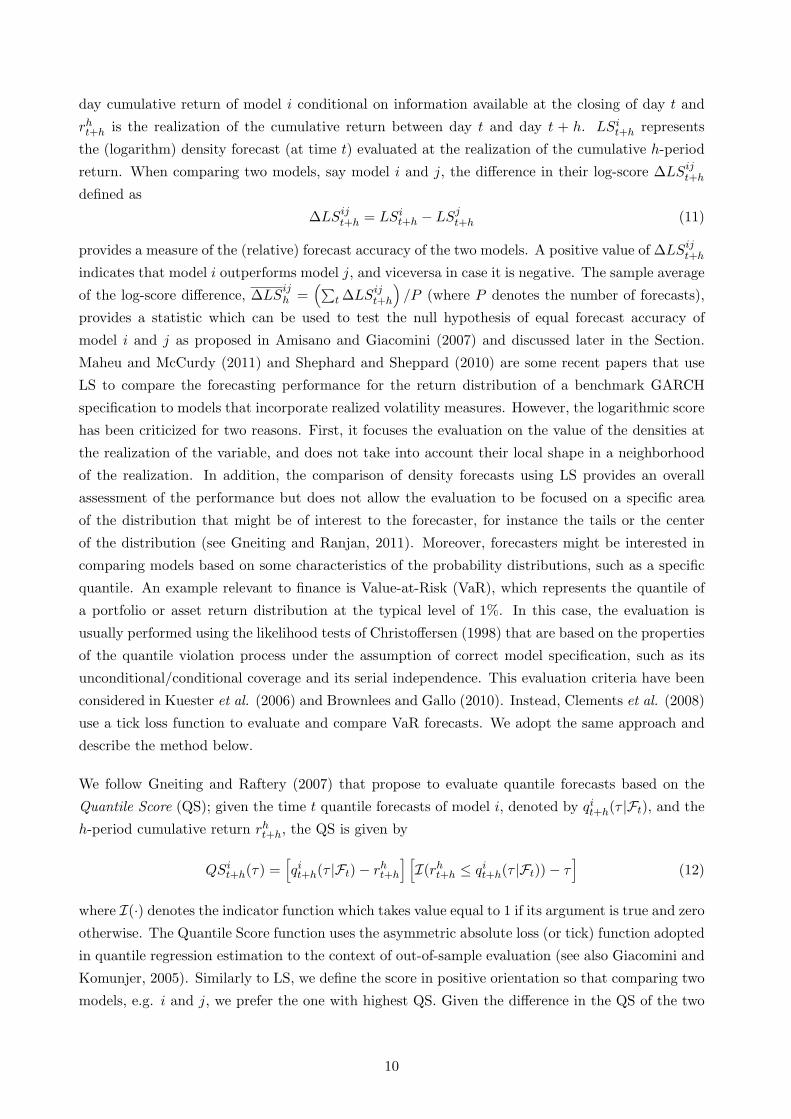
day cumulative return of model i conditional on information available at the closing of day t and

rht+h is the realization of the cumulative return between day t and day t + h. LSit+h represents

the (logarithm) density forecast (at time t) evaluated at the realization of the cumulative h-period

return. When comparing two models, say model i and j, the difference in their log-score ∆LSijt+hdefined as

∆LSijt+h = LSit+h − LSjt+h (11)

provides a measure of the (relative) forecast accuracy of the two models. A positive value of ∆LSijt+hindicates that model i outperforms model j, and viceversa in case it is negative. The sample average

of the log-score difference, ∆LSijh =(∑

t ∆LSijt+h)/P (where P denotes the number of forecasts),

provides a statistic which can be used to test the null hypothesis of equal forecast accuracy of

model i and j as proposed in Amisano and Giacomini (2007) and discussed later in the Section.

Maheu and McCurdy (2011) and Shephard and Sheppard (2010) are some recent papers that use

LS to compare the forecasting performance for the return distribution of a benchmark GARCH

specification to models that incorporate realized volatility measures. However, the logarithmic score

has been criticized for two reasons. First, it focuses the evaluation on the value of the densities at

the realization of the variable, and does not take into account their local shape in a neighborhood

of the realization. In addition, the comparison of density forecasts using LS provides an overall

assessment of the performance but does not allow the evaluation to be focused on a specific area

of the distribution that might be of interest to the forecaster, for instance the tails or the center

of the distribution (see Gneiting and Ranjan, 2011). Moreover, forecasters might be interested in

comparing models based on some characteristics of the probability distributions, such as a specific

quantile. An example relevant to finance is Value-at-Risk (VaR), which represents the quantile of

a portfolio or asset return distribution at the typical level of 1%. In this case, the evaluation is

usually performed using the likelihood tests of Christoffersen (1998) that are based on the properties

of the quantile violation process under the assumption of correct model specification, such as its

unconditional/conditional coverage and its serial independence. This evaluation criteria have been

considered in Kuester et al. (2006) and Brownlees and Gallo (2010). Instead, Clements et al. (2008)

use a tick loss function to evaluate and compare VaR forecasts. We adopt the same approach and

describe the method below.

We follow Gneiting and Raftery (2007) that propose to evaluate quantile forecasts based on the

Quantile Score (QS); given the time t quantile forecasts of model i, denoted by qit+h(τ |Ft), and the

h-period cumulative return rht+h, the QS is given by

QSit+h(τ) =[qit+h(τ |Ft)− rht+h

] [I(rht+h ≤ qit+h(τ |Ft))− τ

](12)

where I(·) denotes the indicator function which takes value equal to 1 if its argument is true and zero

otherwise. The Quantile Score function uses the asymmetric absolute loss (or tick) function adopted

in quantile regression estimation to the context of out-of-sample evaluation (see also Giacomini and

Komunjer, 2005). Similarly to LS, we define the score in positive orientation so that comparing two

models, e.g. i and j, we prefer the one with highest QS. Given the difference in the QS of the two

10

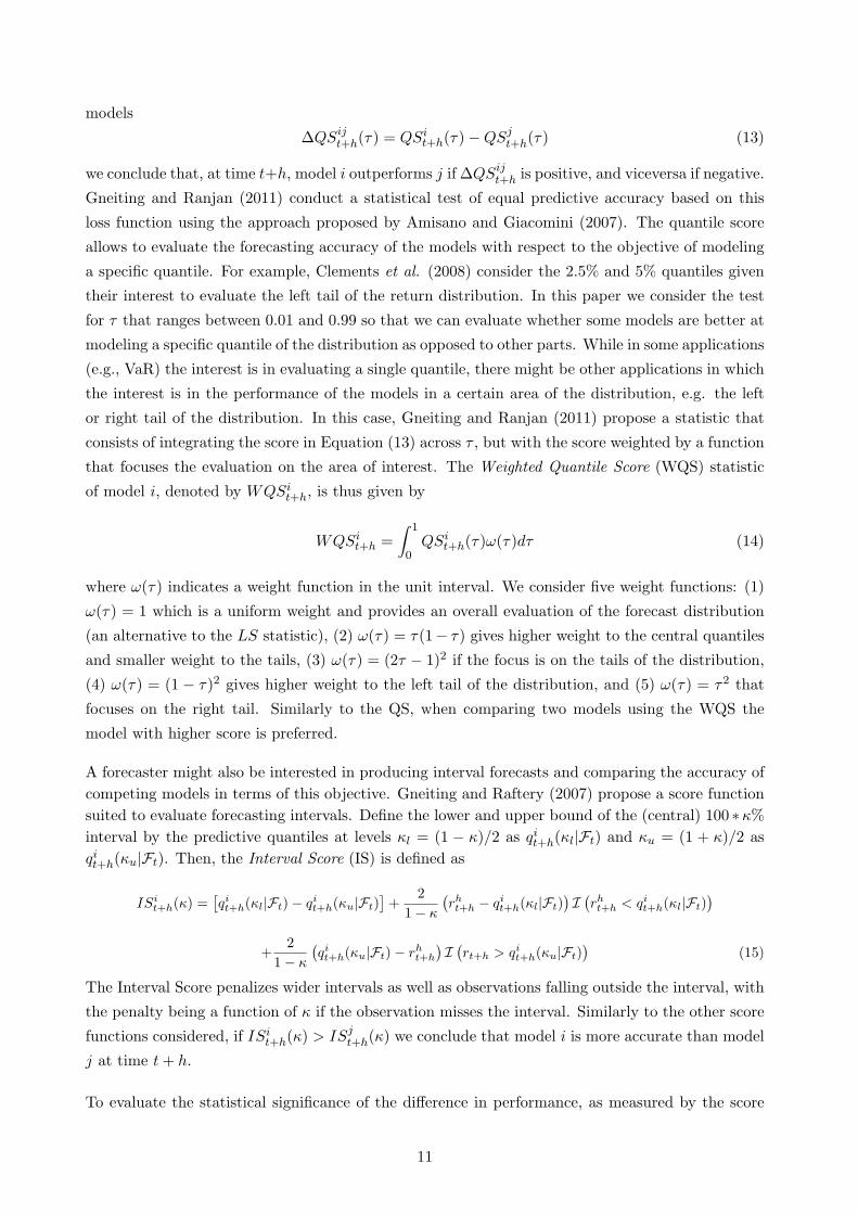
models

∆QSijt+h(τ) = QSit+h(τ)−QSjt+h(τ) (13)

we conclude that, at time t+h, model i outperforms j if ∆QSijt+h is positive, and viceversa if negative.

Gneiting and Ranjan (2011) conduct a statistical test of equal predictive accuracy based on this

loss function using the approach proposed by Amisano and Giacomini (2007). The quantile score

allows to evaluate the forecasting accuracy of the models with respect to the objective of modeling

a specific quantile. For example, Clements et al. (2008) consider the 2.5% and 5% quantiles given

their interest to evaluate the left tail of the return distribution. In this paper we consider the test

for τ that ranges between 0.01 and 0.99 so that we can evaluate whether some models are better at

modeling a specific quantile of the distribution as opposed to other parts. While in some applications

(e.g., VaR) the interest is in evaluating a single quantile, there might be other applications in which

the interest is in the performance of the models in a certain area of the distribution, e.g. the left

or right tail of the distribution. In this case, Gneiting and Ranjan (2011) propose a statistic that

consists of integrating the score in Equation (13) across τ , but with the score weighted by a function

that focuses the evaluation on the area of interest. The Weighted Quantile Score (WQS) statistic

of model i, denoted by WQSit+h, is thus given by

WQSit+h =∫ 1

0QSit+h(τ)ω(τ)dτ (14)

where ω(τ) indicates a weight function in the unit interval. We consider five weight functions: (1)

ω(τ) = 1 which is a uniform weight and provides an overall evaluation of the forecast distribution

(an alternative to the LS statistic), (2) ω(τ) = τ(1− τ) gives higher weight to the central quantiles

and smaller weight to the tails, (3) ω(τ) = (2τ − 1)2 if the focus is on the tails of the distribution,

(4) ω(τ) = (1 − τ)2 gives higher weight to the left tail of the distribution, and (5) ω(τ) = τ2 that

focuses on the right tail. Similarly to the QS, when comparing two models using the WQS the

model with higher score is preferred.

A forecaster might also be interested in producing interval forecasts and comparing the accuracy ofcompeting models in terms of this objective. Gneiting and Raftery (2007) propose a score functionsuited to evaluate forecasting intervals. Define the lower and upper bound of the (central) 100 ∗κ%interval by the predictive quantiles at levels κl = (1 − κ)/2 as qit+h(κl|Ft) and κu = (1 + κ)/2 asqit+h(κu|Ft). Then, the Interval Score (IS) is defined as

ISit+h(κ) =

[qit+h(κl|Ft)− qi

t+h(κu|Ft)]

+2

1− κ(rht+h − qi

t+h(κl|Ft))I(rht+h < qi

t+h(κl|Ft))

+2

1− κ(qit+h(κu|Ft)− rh

t+h

)I(rt+h > qi

t+h(κu|Ft))

(15)

The Interval Score penalizes wider intervals as well as observations falling outside the interval, with

the penalty being a function of κ if the observation misses the interval. Similarly to the other score

functions considered, if ISit+h(κ) > ISjt+h(κ) we conclude that model i is more accurate than model

j at time t+ h.

To evaluate the statistical significance of the difference in performance, as measured by the score

11

functions, we follow the approach of Giacomini and White (2006) and Amisano and Giacomini

(2007). Denote by Sit+h(·) any of the score functions discussed above for model i, and by Sjt+h(·)the score of model j. Then a test statistic for the null hypothesis of equal average forecast accuracy

of the two models, Sit+h(·) = Sjt+h(·) for t = 1, · · · , P , is given by

t = ∆Sijh (·)/σ̂ (16)

where ∆Sijh denotes the difference in the sample mean of the scores and σ̂ represents the HAC

standard error of the difference in scores. The test statistic t is asymptotically standard normal and

rejections for negative values of the statistic indicate that model j significantly outperforms model

i (and vice-versa for positive values).

5 Application

The intra-day dataset was provided by Price-Data and consists of five-minute prices for the S&P

500 futures (SP) and 30-year US Treasury bond futures (US) contracts from January 2, 1990 to

September 9, 2009 (4958 daily observations). The five-minute prices for the SP contracts cover the

time interval from 9:35 to 16:15 (EST), which corresponds to 80 non-overlapping return observations

per day, while the US contracts span the interval from 8:25 to 15:00 (EST), resulting in 79 intra-day

returns2. Figure (1) shows the time series of the daily realized variance for the two assets and

Table (1) reports the summary statistics for the daily squared returns and the realized measures

discussed in Section (2). The evidence indicates that the realized volatility of the equity index

returns is higher and significantly more variable relative to the volatility of the bond futures returns.

In addition, the Table shows that the realized measures RVt, RV (2)t and Ct have lower mean and

variability compared to both the squared returns and RV Nt, which accounts for the overnight

returns. We start the out-of-sample forecasting exercise on January 3, 2000 (for a total of 2419

forecasts) and the model parameters are estimated on a rolling window of 2463 days (approximately

10 years of data). We consider forecast horizons of 1-, 2- and 5-day ahead while the results for 10-

and 20-day are not reported because they are qualitatively similar to the results for 5-day ahead.

This Section is organized as follows. We first present the results of the comparison of the GARCH-

type specifications discussed in Section (3.1). The aim is to select the most accurate forecasting

model for SP and US returns to be considered as the benchmark model. We then discuss the

findings on the forecast performance of the realized volatility models in comparison to the benchmark

GARCH model.

5.1 Benchmark GARCH models

The combination of different conditional variance specifications and assumptions on the error dis-

tribution discussed in Section (3.1) produces a large number of models. We decided to limit the

scope of the comparison to the following cases:2This is the same dataset used by Andersen et al. (2011), with the only difference that we consider a longer period

that includes several recessions and financial turmoil.

12

1. GARCH(1,1): GARCH(1,1) model with standard normal innovations

2. GARCH(1,1)-t: GARCH(1,1) model with tk innovations

3. GARCH(1,1)-EDF: FHS with a GARCH(1,1) conditional variance

4. EGARCH(1,1)-EDF: FHS with a EGARCH(1,1) conditional variance

5. GJR: GJR-GARCH(1,1) with standard normal innovations

6. GJR-EDF: FHS with a GJR-GARCH(1,1) conditional variance

The first three models share the same conditional variance specification but differ in the distribu-

tional assumption for the error term. The remaining models allow for the leverage effect which

is combined with normal errors or with errors resampled from the EDF. In this case we choose

the number of replications B equal to 10000. In comparing these volatility models, we use the

GARCH(1,1)-EDF and GJR-EDF as the benchmark models against which we evaluate the remain-

ing five models. We evaluate the density, quantile and interval forecasts generated by these models

using the predictive accuracy tests discussed in Section (4). In all cases, the test statistics are

standard normal distributed and rejections of the null hypothesis of equal (average) accuracy for

negative values indicate that the benchmark model (GARCH(1,1)-EDF or GJR-EDF) is (signifi-

cantly) outperformed by the alternative model.

S&P 500 Return (SP)

Table (2) shows the t-statistic of the Log-Score (LS) and the Weighted Quantile Score (WQS)

for h equal to 1, 2, and 5. Two findings emerge from the comparison of the volatility models to

the GARCH(1,1)-EDF benchmark. First, the positive LS test statistics obtained by comparing

the benchmark to the GARCH(1,1) model with normal and t distributed errors suggest that these

models are significantly less accurate (compared to the benchmark) at all forecast intervals h. Similar

findings are provided by the WQS with uniform weight at the 1 and 5 day horizons. In addition,

the WQS statistics show that, at all horizons, the GARCH(1,1)-EDF has similar performance to

the models with normal and t distributed errors on the left tail of the return distribution, but it

is significantly more accurate on the right tail. It is thus the case that the three distributional

assumptions provide similarly accurate forecasts when modeling negative returns, but the EDF

assumption provides more precise forecasts of the right tail compared to the parametric distributions.

This suggests that in the forecasting period 2000-2009 the (out-of-sample) evidence does not support

the use of the t distribution for the error term. In addition, the nonparametric nature of the EDF

allows to capture some asymmetry in the error distribution which is not accounted for by the

parametric distributional assumptions. Comparing the GARCH(1,1)-EDF to the EGARCH and

GJR models, it appears that the LS and WQS-uniform tests are significantly negative at the 1

and 2 day horizons, but only the GJR-EDF specification outperforms the benchmark for h=5.

Furthermore, at the 1-day horizon we observe rejections for negative values of the WQS focused

on the left and right tails, but mostly on the right tail for h=2 and at the 5-day horizon. Hence,

including a leverage effect in the conditional variance specification is important in modeling the

return distribution, but this effect seems less pronounced when the object of interest is the multi-

period cumulative return. When considering the GJR-EDF model as the benchmark, the Table

13

shows that in only one case it is outperformed by the EGARCH(1,1)-EDF using the LS test for

h=1, although in all other cases the test statistics are positive and mostly significant. The WQS test

focused on the left and right tail shows that the GJR-EDF outperforms the alternative specifications

on the right tail (as it was the case for the GARCH(1,1)-EDF case), while it provides forecast

accuracy similar to the other asymmetric specifications on the left tail.

The results for the QS(τ) test in Table (3) provide a detailed analysis of the performance of the

competing GARCH models in forecasting the individual quantiles. For the 1% quantiles the results

suggest that all the models considered perform similarly. However, at quantile levels between 5

and 20% the GARCH(1,1)-EDF is significantly outperformed by the asymmetric specifications for

h=1 and by the GJR specifications at the 2-day horizon. For h=5 all models are equally accurate.

Furthermore, we find a similar pattern when looking at the top quantiles of the return distribution,

with the only exception of GJR-EDF that outperforms the GARCH(1,1)-EDF also at the longest

forecast horizons. In VaR applications the interest is focused on quantile levels at 1 and 5%, in which

case our results indicate that the GJR-EDF model provides more accurate forecasts, in particular

at the shorter horizons.

The previous discussion holds also for the IS test at the 50% and 90% level reported in Table (4).

The aim in using this score rule is to compare the performance of the GARCH models in providing

accurate interval forecasts. While at the 1-day horizon the GJR-EDF outperforms the GARCH(1,1)

specification and has similar performance to the EGARCH one, at the longer horizons it outperforms

all competing models (significantly positive test statistics). In terms of the unconditional properties

of the intervals, the interval lengths are quite similar across models and they provide a coverage

close to the nominal level for h=1, but there is a slight over-coverage for h=2 and 5.

Based on this evidence, the assumption on the volatility dynamics seems a much more relevant

choice compared to the error distribution. We thus adopt the GJR-EDF as the benchmark in

the comparison with the realized volatility models since it proved the most robust GARCH-type

specification, among the ones considered, to forecast the distribution of S&P 500 futures returns.

T-Bond Return (US)

The results in Tables (5) to (7) for the 30-year Treasury bond futures returns provide a quite different

picture compared to the findings discussed above for the S&P 500 returns. The accuracy tests show

that, overall, the GARCH(1,1)-EDF and GJR-EDF provide similar forecasting performance and

beat all other GARCH models, in particular at the shortest horizons examined. The fact that the

two benchmarks have similar performance indicates that the evidence of a leverage effect in the

bond futures returns is weaker compared to the S&P 500 returns. Considering the WQS test that

focuses on the tails of the distribution, for h=1 the two benchmarks outperform all other models,

but mostly on the right tail at the 5-day horizon. This fact can be further investigated using the

QS(τ) test in Table (6) which shows that the performance of the benchmarks at h=1 on the left part

of the return distribution is quite similar to the alternative models, although the GARCH(1,1)-EDF

is outperformed by some of the models at the 5% quantile. On the right tail of the distribution,

we find that the better performance of the benchmarks is mostly due to the quantile area between

14

0.80 and 0.99 at all forecasting horizons considered. Furthermore, the IS test shows that at the 50

and at the 90% level the GARCH(1,1)-EDF and GJR-EDF outperform most other models, and in

several cases significantly so. In addition, the empirical coverage for h=1 is slightly higher than

50% for all models but gets closer to the nominal level at the longest horizon.

Summarizing the results for the bond futures returns, it seems that the GARCH(1,1)-EDF is a good

benchmark to compare the forecast accuracy of distribution forecast from the realized volatility

models since it proves to perform similarly to the GJR-EDF (which nests the GARCH(1,1)-EDF

model) and outperforms the remaining models.

5.2 Realized volatility models

In this Section, we address the issue of the relevance of employing realized volatility measures to

forecast the return distribution in comparison to using a GARCH-type volatility model. As discussed

above, the selected benchmark for the S&P 500 futures returns is the GJR-EDF model, while the

absence of asymmetry in the volatility process for the 30-year US T-bond returns suggests that

the GARCH(1,1)-EDF is a satisfactory choice. Similarly to the previous Section, a negative test

statistic indicates that the respective realized volatility model outperforms the GARCH benchmark,

and the opposite when the statistic is positive.

S&P 500 Return (SP)

Table (8) shows that at the 1-day horizon both the LS and WQS-uniform tests indicate that using the

square root of realized volatility measure, rvt, in the HAR-type and the asymmetric specifications

delivers significantly more accurate forecasts compared to GJR-EDF, but not when rvt is smoothed

using EWMA. Moreover, the WQS also indicates that the HAR-type specifications outperform

GJR on the center and right tail of the return distribution, but not significantly on the left tail.

Similar results are also obtained when the high-frequency measure used is rv(2)t, ct, and ct jointly

with the jump component jt. The comparable accuracy of the models based on ct and ct together

with jt thus suggests that separating the jump component does not provide higher accuracy of the

distribution forecasts. We also find that the rvnt measure that accounts for the overnight return

does not outperform the benchmark in any of the tests considered. In addition, the evidence does

not indicate that using squared returns or the VIX index in a HAR-type specification provides better

performance (compared to the time series benchmark). In fact, when using the smoothed squared

returns the test statistics are significantly positive, suggesting that the distribution forecasts are

less accurate compared to the GJR-EDF model. This shows that, once we control for the semi-

parametric modeling assumption, high-frequency measures of volatility contain relevant information

that is useful in forecasting the next day return distribution compared to using squared returns or

a GARCH-type model. However, when we forecast the 2 and 5-day cumulative returns the results

are less supportive of the realized volatility models. In particular, for h=2 some of the specifications

that use RVt still outperform the GJR-EDF forecasts, but at h=5 there is no significant difference

between the realized volatility models and the benchmark, and in fact they provide significantly

worse forecasts in some cases.

15

In summary, the comparison using the LS and WQS-uniform tests shows that some of the realized

volatility models deliver better distribution forecasts (at least at the 1-day horizon), and the analysis

of the local WQS suggests that the improvement is mostly driven by their higher accuracy (compared

to the benchmark) on the right tail of the return distribution. This can be further examined

in Table (9) that reports the QS(τ) test: at the 1-day horizon, the realized volatility measures

outperform the benchmark for quantile levels between 0.70 and 0.95, except when using rvnt. Also

using V IXt provides more accurate quantile forecasts than GJR-EDF on the right tail, but this is

not the case when using squared returns that, in both specifications considered, have significantly

positive test statistics. On the left side of the return distribution, only models that allow for the

asymmetric effect of et and rt beat the benchmark at the 0.20 and 0.30 levels. This is an interesting

result since these asymmetric specifications are able to provide more accurate forecasts at both

low and high quantiles relative to a benchmark model that already accounts for the asymmetric

response of volatility to surprises, although in a parametric form. The QS(τ) test also shows that

the only case in which incorporating the overnight return in RV Nt outperforms the benchmark is

for τ=0.01. At the 2-day horizon, the results show that some realized volatility models outperform

the GJR model at τ=0.01 as well as for high quantile levels. However, at h=5 we do not find any

evidence that the realized volatility models are more accurate compared to the benchmark.

The comparison of the interval forecasts provided in Table (10) suggests that the models based

on realized measures (with the exception of rvnt) outperform the benchmark at the 1-day horizon

at both the 50% and 90% level. At the 2-day horizon several realized volatility models are also

significant when forecasting the 90% interval, but at the 5-day horizon the GJR-EDF significantly

outperforms all quantiles models for 50% intervals and has similar accuracy when forecasting 90%

intervals. However, our conclusions would have been different if we adopted, as several related

papers do, a GARCH(1,1) model as the benchmark. In Table (11) we present the QS(τ) test that

evaluates the performance of the realized volatility models in comparison to the GARCH(1,1)-EDF

benchmark. The most relevant difference, relative to the comparison with the GJR benchmark,

occurs on the left tail of the distribution. In this case, all realized volatility models outperform the

benchmark when forecasting the 5% quantile and most continue to be more accurate for quantile

levels up to 20% for 1 and 2-day ahead forecasts, due to the misspecification of the GARCH(1,1)

model regarding the leverage effect. Furthermore, the quantile model based on the squared returns

performs similarly to the GARCH model at all horizons while the model based on VIX significantly

outperforms the benchmark at high quantiles. These results suggest two conclusions. First, when

evaluating the relative forecast accuracy of different models the choice of the benchmark is essential

and the GJR-EDF model has proved a reliable option to model daily equity returns. In addition,

the quantile-based model combined with the realized volatility measures proves a valuable modeling

approach due to its flexible nature and adaptability to the local (in a quantile sense) dynamics of

the process.

T-Bond Return (US)

The results for the 30-year T-Bond returns are provided in Tables (12) to (14). In this case, the

return quantile models are compared to the GARCH(1,1)-EDF model that was established above

16

as a plausible benchmark. All the statistics used in the forecast comparison point to the conclusion

that realized volatility models do not outperform the GARCH(1,1) benchmark, even at the shortest

horizon of 1-day. In fact, the realized volatility models are outperformed by the benchmark in the

center of the distribution (as evaluated by the WQS) at the 5-day horizon. In addition, the quantile

models based on the smoothed squared returns have also similar accuracy relative to the benchmark,

thus suggesting that for bond returns there is no added value in considering the high-frequency

volatility measures. The only case in which the quantile models outperform the benchmark is when

evaluating the 1% quantile for which several realized volatility models outperform the benchmark.

However, both approaches provide similar results in terms of interval coverage and average length

of the intervals.

6 Discussion

The results discussed above suggest that the realized volatility quantile model provides more accu-

rate distribution, quantile and interval forecasts compared to the GJR-EDF and GARCH(1,1)-EDF

when predicting the S&P 500 returns at short horizons. To explain these findings, we construct

measures of volatility, skewness and kurtosis that characterize the distribution of financial returns

based on the estimated quantiles of the different models. An advantage of deriving these mea-

sures from the quantiles is that they inherit the property of being conditional on the information

available at the time the forecast is made. In addition, the quantile-based measures are typically

regarded as robust to the effect of large returns and outliers compared to averaging powers of the

returns. As a quantile-based proxy for volatility we use the Interquartile Range (IQR) which is

defined as IQRt,h = qt,h(0.75) − qt,h(0.25), where IQRt,h denotes the IQR forecast made in day

t at the horizon h and qt+h(τ |Ft) represents the conditional quantile at levels τ = 0.25 and 0.75.

The IQR can also be interpreted as the 50% forecast interval for the returns which was statistically

evaluated in the previous Section. In addition, we consider the 95% forecast interval obtained as

qt,h(0.975) − qt,h(0.025), which relies on the extreme quantiles and might highlight relevant differ-

ences between the forecasting models in the tails of the return distribution. Furthermore, we follow

Kim and White (2004) and define robust skewness and kurtosis measures based on quantiles. The

h-day ahead Skewness forecast in day t, denoted by SKt,h, is defined as

SKt,h =qt,h(0.75) + qt,h(0.25)− 2qt,h(0.5)

IQRt,h(17)

while the Kurtosis forecast, denoted by Kt,h, is obtained as

Kt,h =qt,h(0.975)− qt,h(0.025)

IQRt,h− 2.91 (18)

Figure (2) shows the time series forecasts of these four quantities for the S&P 500 futures returns

with h = 1 from January 3, 2000 until September 9, 2009 (2419 days). We confine the comparison

to the GARCH(1,1)-EDF, the GJR-EDF, and the quantile model with regressors given by rvt, rvwtand rvmt . The realized volatility RVt was found to perform similarly to the other realized volatility

measures. Looking at panel (a) and (b) of the Figure, it appears that the quantile model (right plot)

17

provides wider intervals compared to the GARCH models (left and center plot) during the 2008-2009

financial instability period. In interpreting the skewness and kurtosis of the GARCH(1,1)-EDF and

GJR-EDF models we should recall that the error distribution is drawn from the EDF and can thus

display unconditional skewness and kurtosis, in addition to the fact that the estimation is performed

on a rolling window. For both parametric models, the skewness forecast is slightly above zero at the

beginning of the forecasting period and trends toward -0.1 at the end of the sample. Instead, for

the quantile model the skewness forecast oscillates around zero with a persistent negative deviation

in the 2005-2009 period when it reached the lowest value of -0.2. As concerns the kurtosis, the two

GARCH specifications provide qualitatively similar results with the kurtosis forecasts starting above

4 at the beginning of the sample and trending downward until the end of 2005 when it increased

again. On the other hand, the kurtosis forecast from the quantile model varies significantly more

in the range 2.5 to 4 suggesting that the shape of the distribution forecast is more responsive to

market conditions.

To further investigate the relationship between these measures and the properties of the return

distribution, in Figure (3) we report non-parametric estimates of the four measures against the

forecast realization, rt+1, using a kernel smoother with a rule-of-thumb bandwidth and trimming

the 1% most extreme return observations. The aim is to compare the measures derived from the

different forecasting models and relate them to the statistical evidence based on the QS(τ), WQS

and IS tests discussed in the previous Section. Panel (a) of Figure (3) shows that the realized

volatility model predicts larger interquartile ranges (compared to the two parametric models) when

the return realization happens to be large and negative, but only slightly larger relative to the

GJR-EDF forecasts when returns are large and positive. In both tails, the GARCH(1,1)-EDF

model provides ranges that are typically smaller than the other two models. In addition, the three

models provide similar IQR forecasts at the center of the return distribution. It seems thus that the

evidence in Table (10) indicating the higher accuracy of the 50% interval forecasts of the quantile

model (compared to GJR-EDF) is driven by the fact that it predicts larger ranges when extreme (in

particular negative) returns actually occur compared to the GARCH models. However, the situation

is reversed when considering the 95% interval in panel (b) since the quantile model forecasts are

smaller compared to both GARCH models, and in particular at the center and right tail of the

return distribution. Hence, these results indicate that, in days in which the (absolute) return is

large, the quantile model forecasts a distribution which is wider at the center and narrower in the

tails, compared to the GARCH models. It is thus not surprising that the quantile model predicts

distributions with lower kurtosis in the tails of the return distribution as shown in panel (d) of the

Figure, which can be attributed to the smaller 95% intervals and larger 50% intervals (compared to

GJR-EDF) that are the numerator and denominator, respectively, of the kurtosis measure defined

in Equation (18). On the other hand, when the return occurs at the center of the distribution the

forecasts have comparable characteristics as demonstrated by the similar kurtosis of the quantile

and the GJR-EDF models. In terms of the skewness in panel (c), it seems to have no dependence

with the return distribution.

To better understand these findings, in Figure (4) we report the non-parametric estimates of the

relationship between the quantiles (for τ equal to 0.025, 0.25, 0.75, and 0.975) that are used in the

18

IQR, skewness and kurtosis definitions and the forecast realization, rt+1. Looking at panels (a) and

(b) of the Figure, it appears that the wider interquartile range for large negative returns can be

mostly attributed to the difference in the 75% quantile forecasts of the models considered and, to a

lesser extent, to the 25%. In addition, we also find that for large positive returns, the 25% quantile of

the realized volatility model and the GJR-EDF are quite similar while the 75% quantiles moderately

deviate. Similarly, the fact that the 95% interval forecast of the quantile model is smaller compared

to the GARCH models seems to be almost entirely driven by the quantile at τ = 0.025 rather than

the 97.5% quantile (panel (c) and (d) in the Figure).

The empirical analysis of the previous Section has also indicated that the quantile model with

regressors given by the absolute return and its weekly and monthly moving averages is equally

accurate compared to the GJR-EDF in predicting the S&P 500 returns. We thus conduct a similar

analysis to the one above, in which we intend to compare the characteristics of the distribution

forecasts of the quantile model with regressors rt|, |rt|w, and |rt|m to the GARCH benchmarks. In

Figure (5) we report the kernel estimates of the relationship between the IQR, 95% interval, skewness

and kurtosis and the forecast realization, rt+1, while in Figure (6) we report the selected quantiles

for τ equal to 0.025, 0.25, 0.75, and 0.975. Panel (a) of Figure (5) shows that the interquartile range

forecast of the GJR-EDF and the quantile model almost coincide, but differ from the GARCH(1,1)-

EDF, mostly in the tails. This result is due to the fact that the 25% and the 75% quantiles of

the two models are very similar as shown in panels (a) and (b) of Figure (6). The 95% interval

forecasts and the kurtosis of the quantile model are slightly smaller compared to GJR-EDF (see

panel (b) and (d) of Figure 5), mostly as a result of the difference of the τ = 0.025 quantile.

The close relationship between the quantiles (except at the lowest level) confirms the ability of

the semi-parametric model to provide forecasts of similar to the best GARCH-type model, without

introducing parametric assumptions on the volatility dynamics and the error distribution. Overall,

these results suggest that the quantile approach provides the modeling flexibility required to account

for possible asymmetries, or more generally nonlinearities, in the conditional distribution of returns,

but also that considering realized measures of volatility is essential to outperform parametric models

in forecasting returns.

7 Conclusion

The distribution of financial returns is a relevant object in financial decision-making, since it pro-

vides a complete characterization of the future outcomes and allows to derive quantities of interest

to a forecaster, such as quantiles, intervals, and volatility. In this paper we adopt a quantile re-

gression framework which represents a natural way to make the conditional distribution of future

returns depend on current information. In particular, we consider realized measures of volatility

as the driving force behind the variation over time of the return quantiles. The model has several

advantages, among others the fact that it does not require assumptions on the error distribution

as well as its adaptability in terms of the explanatory variables and their effects on different parts

of the return distribution. To assess the merit of the model, we compare it to several GARCH

models in which the variation of the return distribution is restricted to occur parametrically in the

19

second moment. In addition, shifting the focus of the forecast exercise from the volatility process

to the distribution allows an in-depth comparison of forecasts from different models in terms of

distribution or density but also in terms of quantities like the quantiles or intervals.

A first result that emerges from our analysis is that the realized volatility quantile model outperforms

an asymmetric GARCH specification in forecasting the S&P 500 returns, mostly at the 1 and 2-day

horizons and on the right tail of the return distribution. On the other hand, we also find that the

quantile model (significantly) outperforms the GARCH(1,1) model on both tails of the S&P 500

return distribution. These results highlight the two main characteristics of the proposed approach.

The flexibility of the quantile model allows to easily adapt to the properties of the data without

having to specify a parametric model and a distribution for the error term. In addition, using the

realized measures of volatility provides valuable information (in a forecasting sense) compared to

the information extracted from the time series of returns using a GARCH model. To further stress

the relevance of the high-frequency measures to the forecasting success, we also consider a quantile

model in which the realized volatility estimators are replaced by the absolute daily returns. In this

case, the quantile forecasts are (in most cases) equally accurate to the GARCH benchmark models

and in some cases significantly worse, hence indicating that the semi-parametric method alone does

not deliver more precise distribution and quantile forecasts. On the other hand, the semi-parametric

model performs similarly to the benchmark GARCH model when considering the bond returns, thus

suggesting that the realized measures do not provide additional predictive content compared to a

parametric volatility filter (e.g., a GARCH(1,1) model). Another fact emerging from our analysis is

that the various realized measures considered in the paper perform very similarly in terms of forecast

accuracy. The refinements introduced to account for microstructure noise and the separation of the

continuous path variability from the jump component do not provide better performance in an

out-of-sample forecasting context compared to using the simple realized volatility measure.

Overall, our results confirm the usefulness of including realized measures of volatility, in particular

for the S&P 500 at short forecast horizons. However, when forecasting the equity returns at long

horizons and the bond returns (at all horizons) a GARCH-type model provides reasonably accurate

forecasts. These results might be considered at odds with the earlier findings in the literature that

models based on realized volatility measures dominate (in- and out-of-sample) volatility forecasts

obtained from parametric time series models. These opposing findings can be attributed to the

difference in the object being forecast (distribution, quantile and interval rather than volatility) as

well as to the loss functions adopted in the evaluation. In addition, since Andersen and Bollerslev

(1998) the realized volatility literature has typically evaluated and compared realized volatility and

GARCH models on their ability to forecast realized volatility rather than squared returns. This

approach is not feasible in the context of quantile or interval forecasts evaluation since there are no

methods available to construct realized counterparts for these quantities. In this sense, we put back

the returns in the evaluation process which can (partly) explain the difference in results compared to

the earlier papers. However, it can be argued that our forecast comparison is relative to a benchmark

model and thus should be less sensitive to the issue as opposed to an absolute performance criterion.

20

References

Ait-Sahalia, Y., Mykland, P.A. and Zhang, L. (2005a). How often to sample a continuous-timeprocess in the presence of market microstructure noise. Review of Financial Studies, 18, 351–416.

Ait-Sahalia, Y., Mykland, P.A. and Zhang, L. (2005b). A tale of two time scales: Determining inte-grated volatility with noisy high-frequency data. Journal of the American Statistical Association,100, 1394–1411.

Amisano, G. and Giacomini, R. (2007). Comparing density forecasts via Weighted Likelihood RatioTests. Journal of Business & Economic Statistics, 25, 177–190.

Andersen, T.G. and Bollerslev, T. (1998). Answering the skeptics: Yes, standard volatility modelsdo provide accurate forecasts. International Economic Review, 39, 885–905.

Andersen, T.G., Bollerslev, T. and Diebold, F.X. (2007). Roughing it up: including jump compo-nents in the measurement, modeling and forecasting of return volatility. Review of Economicsand Statistics, 89, 701–720.

Andersen, T.G., Bollerslev, T., Diebold, F.X. and Ebens, H. (2001a). The distribution of realizedstock return volatility. Journal of Financial Economics, 61, 43–76.

Andersen, T.G., Bollerslev, T., Diebold, F.X. and Labys, P. (2001b). The distribution of realizedexchange rate volatility. Journal of the American Statistical Association, 96, 42–55.

Andersen, T.G., Bollerslev, T., Diebold, F.X. and Labys, P. (2003). Modeling and forecastingrealized volatility. Econometrica, 71, 529–626.

Andersen, T.G., Bollerslev, T. and Huang, X. (2011). A reduced form framework for modelingvolatility of speculative prices based on realized variation measures. Journal of Econometrics,160, 176–189.

Bali, T., Mo, H. and Tang, Y. (2008). The role of autoregressive conditional skewness and kurtosisin the estimation of conditional var. Journal of Banking and Finance, 32, 269–282.

Bandi, F.M. and Russell, J.R. (2008). Microstructure noise, realized volatility, and optimal sam-pling. Review of Economic Studies, 75, 339–369.

Bao, Y., Lee, T.-H. and Saltoglu, B. (2007). Comparing density forecast models. Journal ofForecasting, 26, 203–225.

Barndorff-Nielsen, O.E., Hansen, P.R., Lunde, A. and Shephard, N. (2008). Designing realizedkernels to measure the ex-post variation of equity price in the presence of noise. Econometrica,76, 1481–1536.

Barndorff-Nielsen, O.E. and Shephard, N. (2002a). Econometric analysis of realised volatility andits use in estimating stochastic volatility models. Journal of the Royal Statistical Society B, 64,253–280.

Barndorff-Nielsen, O.E. and Shephard, N. (2002b). Estimating quadratic variation using realisedvolatility. Journal of Applied Econometrics, 17, 457–477.

Barndorff-Nielsen, O.E. and Shephard, N. (2004). Power and bipower variation with stochasticvolatility and jumps. Journal of Financial Econometrics, 2, 1–48.

Barone-Adesi, G., Engle, R.F. and Mancini, L. (2011). A GARCH option pricing model with filteredhistorical simulation. Review of Financial Studies, 24, 1223–1258.

Becker, R., Clements, A.E. and White, S.I. (2007). Does implied volatility provide any informationbeyond that captured in model-based volatility forecasts? Journal of Banking and Finance, 31,2535–2549.

Blair, B.J., Poon, S-H. and Taylor, S.J. (2001). Forecasting S&P 100 volatility: the incrementalinformation content of implied volatilities and high-frequency index returns. Journal of Econo-metrics, 105, 5–26.

Bollerslev, T. (1986). Generalized Autoregressive Conditional Heteroskedasticity. Journal of Econo-metrics, 31, 307–327.

21

Bollerslev, T., Kretschmer, U., Pigorsch, C. and Tauchen, G. (2009). A discrete-time model for dailyS&P500 returns and realized variations: Jumps and leverage effects. Journal of Econometrics,150, number 2, 151 – 166.

Brownlees, C.T. and Gallo, G.M. (2010). Comparison of volatility measures: a risk managementperspective. Journal of Financial Econometrics, 8, 29–56.

Christoffersen, P. (1998). Evaluating interval forecasts. International Economic Review, 39, 841–862.

Clements, M.P., Galvao, A.B. and Kim, J.H. (2008). Quantile forecasts of daily exchange ratereturns from forecasts of realized volatility. Journal of Empirical Finance, 15, 729–750.

Corsi, F. (2009). A simple approximate long-memory model of realized volatility. Journal ofFinancial Econometrics, 7, 174–196.

Diebold, F.X., Gunther, T.A. and Tay, A.S. (1998). Evaluating density forecasts with applicationto financial risk management. International Economic Review, 39, 863–883.

Engle, R.F. (1982). Autoregressive conditional heteroskedasticity with estimates of variance ofUnited Kingdom inflation. Econometrica, 50, 987–1007.

Engle, R.F. and Gallo, G.M. (2006). A multiple indicators model for volatility using intra-dailydata. Journal of Econometrics, 131, 3–27.

Engle, R.F. and Manganelli, S. (2004). CAViaR: Conditional autoregressive value at risk byregression quantiles. Journal of Business and Economic Statistics, 22, 367–381.

Gaglianone, W.P., Lima, L.R., Linton, O. and Smith, D.R. (2011). Evaluating Value-at-Risk modelsvia quantile regression. Journal of Business and Economic Statistics, 29, 150–160.

Giacomini, R. and Komunjer, I. (2005). Evaluation and combination of conditional quantile fore-casts. Journal of Business and Economic Statistics, 23, 416–431.

Giacomini, R. and White, H. (2006). Tests of conditional predictive ability. Econometrica, 74,1545–1578.

Glosten, L.R., Jagannathan, R. and Runkle, D.E. (1993). On the relation between the expectedvalue and the volatility of the nominal excess return on stocks. Journal of Finance, 48, 1779–1801.

Gneiting, T. and Raftery, A.E. (2007). Strictly proper scoring rules, prediction, and estimation.Journal of the American Statistical Association, 102, 359–378.

Gneiting, T. and Ranjan, R. (2011). Comparing density forecasts using threshold and quantileweighted scoring rules. Journal of Business and Economic Statistics, 29, 411–422.

Hansen, P.R., Huang, Z. and Shek, H.H. (2011). Realized GARCH: A joint model for returns andrealized measures of volatility. Journal of Applied Econometrics forthcoming.

Hansen, P.R. and Lunde, A. (2005). A comparison of volatility models: Does anything beat aGARCH(1,1)? Journal of Applied Econometrics, 20, 873–889.

Hansen, P.R. and Lunde, A. (2006a). Consistent ranking of volatility models. Journal of Econo-metrics, 131, 97–121.

Hansen, P.R. and Lunde, A. (2006b). Realized variance and market microstructure noise. Journalof Business and Economic Statistics, 24, 127–218.

Huang, X. and Tauchen, G. (2005). The relative contribution of jumps to total price variance.Journal of Financial Econometrics, 3, 456–499.

Kim, T.-H. and White, H. (2004). On more robust estimation of skewness and kurtosis. FinanceResearch Letters, 1, 56–73.

Koenker, R. and Bassett, G. (1978). Regression quantiles. Econometrica, 46, 33–50.

Kuester, K., Mittnik, S. and Paolella, M.S. (2006). Value-at-Risk prediction: A comparison ofalternative strategies. Journal of Financial Econometrics, 4, 53–89.

22

Maheu, J.M. and McCurdy, T.J. (2011). Do high-frequency measures of volatility improve forecastsof return distributions? Journal of Econometrics, 160, 69–76.

Meddahi, N. (2002). A theoretical comparison between integrated and realized volatility. Journalof Applied Econometrics, 17, 479–508.

Nelson, D.B. (1991). Conditional heteroskedasticity in asset returns: a new approach. Econometrica,59, 347–370.

Shephard, N. and Sheppard, K. (2010). Realising the future: forecasting with high-frequency-basedvolatility (HEAVY) models. Journal of Applied Econometrics, 25, 197–231.

Wright, J. and Zhou, H. (2009). Bond risk premia and realized jump risk. Journal of Banking andFinance, 33, 2333–2345.

Xiao, Z. and Koenker, R. (2009). Conditional quantile estimation for generalized autoregressiveconditional heteroscedasticity models. Journal of the American Statistical Association, 104,1696–1712.

Zikes, F. (2010). Semiparametric conditional quantile models for financial returns and realizedvolatility. working paper.

23

1990 1995 2000 2005 2010

02

46

8

RV

(a) S&P 500 (SP)

1990 1995 2000 2005 2010

02

46

8

RV

(b) T-Bond (US)

Figure 1: The time series of the daily realized volatility measure, RVt, in Equation (1) for the S&P 500 futuresreturns (left) and the 30-year Treasury bond futures returns (right) from January 2, 1990 to September 9, 2009.

Table 1: Summary Statistics

r2t RVt RV (2)t RV Nt Jt Ct

SP

Mean 1.43 1.03 0.97 1.38 0.04 0.99S.D. 4.60 2.13 2.09 2.74 0.33 2.04

US

Mean 0.38 0.29 0.27 0.39 0.02 0.26S.D. 0.78 0.37 0.43 0.52 0.16 0.27

Mean and standard deviation (S.D.) for the daily squared returns and the realizedvolatility measures discussed in Section (2) for the S&P 500 futures returns (SP) andthe 30-year T-bond futures returns (US).

24

Table 2: S&P 500 Futures Return

LS WQSuniform center tails left right

h = 1GARCH(1,1)-EDF vs:GARCH(1,1) 1.76 2.29 1.87 2.28 -0.13 3.67GARCH(1,1)-t 2.25 2.59 2.01 2.84 -0.53 4.59EGARCH(1,1)-EDF -4.43 -4.93 -4.40 -4.43 -2.70 -3.50GJR -1.79 -3.02 -2.09 -3.54 -2.30 -2.88GJR-EDF -3.01 -4.73 -4.34 -4.41 -2.27 -4.25

GJR-EDF vs:GARCH(1,1) 3.71 5.87 5.61 4.96 1.85 6.11GARCH(1,1)-EDF 3.01 4.73 4.34 4.41 2.27 4.25GARCH(1,1)-t 4.00 5.73 5.37 5.05 1.62 6.41EGARCH(1,1)-EDF -1.87 -0.66 -1.01 -0.32 -0.04 -0.41GJR 0.70 1.30 1.13 1.14 -0.66 2.39

h = 2GARCH(1,1)-EDF vs:GARCH(1,1) 1.61 1.05 0.42 1.87 -0.59 3.01GARCH(1,1)-t 2.01 1.45 0.64 2.40 -0.73 4.05EGARCH(1,1)-EDF -2.17 -1.97 -2.74 -1.21 -0.19 -1.87GJR -1.72 -3.32 -3.63 -2.84 -1.86 -2.43GJR-EDF -4.06 -4.01 -3.85 -3.76 -1.63 -4.64

GJR-EDF vs:GARCH(1,1) 3.92 4.76 4.91 4.18 1.16 7.43GARCH(1,1)-EDF 4.06 4.01 3.85 3.76 1.63 4.64GARCH(1,1)-t 4.15 4.80 4.78 4.29 1.00 7.79EGARCH(1,1)-EDF 1.37 1.97 0.68 2.94 1.58 2.60GJR 1.76 0.47 -0.53 2.33 -1.13 4.00

h = 5GARCH(1,1)-EDF vs:GARCH(1,1) 3.12 1.95 1.18 3.17 0.40 4.97GARCH(1,1)-t 3.51 2.26 1.47 3.53 -0.01 5.75EGARCH(1,1) 0.66 1.02 0.84 1.07 0.27 1.12EGARCH(1,1)-EDF 2.83 3.27 2.85 3.21 2.50 1.61GJR 0.24 -0.95 -1.03 -0.76 -0.81 -0.24GJR-EDF -1.81 -2.15 -1.18 -2.91 -0.90 -3.84

GJR-EDF vs:GARCH(1,1) 4.10 4.57 3.94 4.04 0.80 9.18GARCH(1,1)-EDF 1.81 2.15 1.18 2.91 0.90 3.84GARCH(1,1)-t 4.29 4.74 4.22 4.17 0.62 9.55EGARCH(1,1) 2.21 2.97 1.67 4.27 1.23 4.78EGARCH(1,1)-EDF 4.42 4.53 3.04 5.71 3.66 5.22GJR 2.42 2.88 0.76 4.40 0.59 5.94

LS refers to the difference in Log Score test in Equation (11) and WQS to the difference in WeightedQuantile Score of Equation (14) for functions that weight the center, tails, left tail, and right tail of thereturn distribution. A negative value indicates that the alternative model outperforms the benchmark (eitherGARCH(1,1)-EDF or GJR-EDF), and the opposite for a positive value. The value reported is the t-statisticas described in Equation (16) which is standard normal distributed. In bold are denoted the test statisticsthat are significantly negative at 5% (one-sided), and in italics the ones that are significantly positive at thesame level. h denotes the forecasting horizon.

25

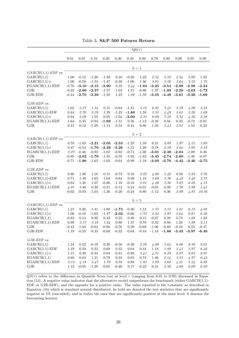
Table 3: S&P 500 Futures Return

QS(τ)

0.01 0.05 0.10 0.20 0.30 0.40 0.60 0.70 0.80 0.90 0.95 0.99

h = 1GARCH(1,1)-EDF vs:GARCH(1,1) 1.08 -0.12 -1.26 -1.39 0.16 -0.20 1.22 2.74 3.18 2.54 2.08 1.33GARCH(1,1)-t 1.00 -0.58 -1.34 -1.47 -0.38 -1.06 1.56 3.01 3.50 3.64 3.52 1.75EGARCH(1,1)-EDF 0.76 -3.10 -3.15 -2.90 0.18 2.44 -1.94 -3.25 -3.54 -2.88 -2.98 -2.24GJR -0.23 -2.96 -2.57 -1.57 1.03 1.15 -0.86 -1.37 -1.93 -2.20 -2.63 -1.73GJR-EDF -0.44 -2.70 -2.39 -1.39 1.23 1.88 -1.59 -3.55 -4.49 -3.61 -3.26 -1.69

GJR-EDF vs:GARCH(1,1) 1.02 2.27 1.74 0.15 -0.64 -1.31 3.12 6.85 7.45 5.39 4.09 2.25GARCH(1,1)-EDF 0.44 2.70 2.39 1.39 -1.23 -1.88 1.59 3.55 4.49 3.61 3.26 1.69GARCH(1,1)-t 0.94 2.08 1.55 0.05 -1.04 -2.00 3.33 6.89 7.22 5.74 4.56 2.28EGARCH(1,1)-EDF 1.64 0.35 -0.94 -1.69 -1.51 0.56 -1.12 -0.20 0.56 0.33 -0.72 -0.91GJR 0.31 0.12 -1.29 -1.14 0.54 0.44 0.86 1.50 2.43 2.01 1.54 0.23

h = 2GARCH(1,1)-EDF vs:GARCH(1,1) 0.78 -1.03 -2.21 -2.05 -2.53 -1.25 1.59 0.31 2.09 1.97 4.21 1.69GARCH(1,1)-t 0.47 -0.54 -1.76 -2.29 -3.26 -1.51 1.38 0.78 2.59 3.04 5.05 3.18EGARCH(1,1)-EDF 2.27 -0.46 -0.93 -1.02 -0.62 -0.74 -1.00 -3.01 -2.40 -2.04 -1.09 0.46GJR -0.68 -2.02 -1.76 -1.45 -0.59 -1.02 -1.62 -3.45 -2.74 -2.60 -1.48 -0.07GJR-EDF -0.71 -1.86 -1.63 -1.03 -0.64 -0.99 -1.18 -3.69 -3.76 -4.42 -3.46 -2.75

GJR-EDF vs:GARCH(1,1) 0.86 1.36 1.16 0.15 -0.73 0.16 3.22 4.08 5.46 6.66 5.83 3.76GARCH(1,1)-EDF 0.71 1.86 1.63 1.03 0.64 0.99 1.18 3.69 3.76 4.42 3.46 2.75GARCH(1,1)-t 0.63 1.38 1.07 -0.06 -1.18 -0.18 2.81 4.20 5.56 7.03 6.28 4.15EGARCH(1,1)-EDF 4.01 1.46 0.39 -0.21 -0.12 0.24 -0.01 -0.65 0.39 1.70 2.99 3.45GJR -0.02 -0.93 -1.04 -1.26 -0.20 -0.24 -0.80 -1.12 0.36 2.09 4.87 10.36

h = 5GARCH(1,1)-EDF vs:GARCH(1,1) 1.21 0.20 -1.41 -1.08 -1.73 -0.30 1.12 1.75 3.15 5.01 6.19 4.08GARCH(1,1)-t 1.00 -0.10 -1.63 -1.47 -2.02 -0.66 1.72 2.22 3.97 5.64 6.61 6.20EGARCH(1,1) -0.83 0.14 0.90 0.43 0.22 0.89 0.15 -0.07 0.28 0.73 1.68 1.68EGARCH(1,1)-EDF 0.99 3.17 3.18 1.64 0.80 1.37 0.70 0.32 0.80 1.28 1.99 2.11GJR -0.42 -1.03 -0.62 -0.66 -0.76 0.20 -0.68 -1.06 -0.60 -0.16 0.23 -0.47GJR-EDF -1.19 -0.59 -0.33 -0.69 -0.32 -0.04 -0.44 -1.18 -1.88 -3.43 -3.97 -6.46

GJR-EDF vs:GARCH(1,1) 1.24 0.52 -0.19 0.28 -0.56 -0.30 2.59 4.08 5.64 8.66 8.50 9.01GARCH(1,1)-EDF 1.19 0.59 0.33 0.69 0.32 0.04 0.44 1.18 1.88 3.43 3.97 6.46GARCH(1,1)-t 1.15 0.39 -0.34 0.04 -0.81 -0.80 3.41 4.51 6.29 8.87 8.63 9.91EGARCH(1,1) 0.88 0.84 1.21 0.78 0.34 0.65 0.74 1.46 2.14 3.53 4.97 6.42EGARCH(1,1)-EDF 3.13 4.18 3.47 1.79 0.78 0.88 1.82 1.89 2.68 4.21 5.34 6.88GJR 1.13 -0.95 -1.28 -0.05 -0.40 0.17 -0.22 0.31 2.26 4.69 6.09 6.30

QS(τ) refers to the difference in Quantile Score test at level τ (ranging from 0.01 to 0.99) discussed in Equa-tion (13). A negative value indicates that the alternative model outperforms the benchmark (either GARCH(1,1)-EDF or GJR-EDF), and the opposite for a positive value. The value reported is the t-statistic as described inEquation (16) which is standard normal distributed. In bold are denoted the test statistics that are significantlynegative at 5% (one-sided), and in italics the ones that are significantly positive at the same level. h denotes theforecasting horizon.

26

Table 4: S&P 500 Futures Return

κ = 50% κ = 90%IS Test Length Coverage IS Test Length Coverage

h = 1GARCH(1,1)-EDF vs 1.52 0.52 4.13 0.91GARCH(1,1) 1.15 1.70 0.55 0.24 4.15 0.91GARCH(1,1)-t 1.14 1.71 0.56 1.23 4.17 0.91EGARCH(1,1) -0.85 1.83 0.58 -2.30 4.44 0.93EGARCH(1,1)-EDF -4.69 1.58 0.53 -4.02 4.22 0.91GJR -2.00 1.73 0.56 -3.36 4.20 0.91GJR-EDF -3.20 1.56 0.53 -3.36 4.18 0.91

GJR-EDF vs 1.56 0.53 4.18 0.91GARCH(1,1) 4.43 1.70 0.55 3.26 4.15 0.91GARCH(1,1)-EDF 3.20 1.52 0.52 3.36 4.13 0.91GARCH(1,1)-t 4.04 1.71 0.56 3.47 4.17 0.91EGARCH(1,1) 0.89 1.83 0.58 1.11 4.44 0.93EGARCH(1,1)-EDF -1.53 1.58 0.53 -0.64 4.22 0.91GJR -0.24 1.73 0.56 -0.06 4.20 0.91

h = 2GARCH(1,1)-EDF vs 2.21 0.49 5.73 0.92GARCH(1,1) -0.62 2.38 0.52 3.00 5.78 0.92GARCH(1,1)-t 0.15 2.39 0.52 3.66 5.82 0.92EGARCH(1,1)-EDF -2.63 2.40 0.52 -0.93 6.23 0.94GJR -2.90 2.41 0.53 -2.27 5.87 0.93GJR-EDF -3.42 2.24 0.50 -3.03 5.76 0.92

GJR-EDF vs 2.24 0.50 5.76 0.92GARCH(1,1) 2.52 2.38 0.52 3.50 5.78 0.92GARCH(1,1)-EDF 3.42 2.21 0.49 3.03 5.73 0.92GARCH(1,1)-t 2.78 2.39 0.52 3.74 5.82 0.92EGARCH(1,1)-EDF -0.72 2.40 0.52 2.74 6.23 0.94GJR -1.30 2.41 0.53 3.55 5.87 0.93

h = 5GARCH(1,1)-EDF vs 3.51 0.51 9.01 0.93GARCH(1,1) 1.39 3.73 0.55 3.98 9.09 0.93GARCH(1,1)-t 1.58 3.75 0.55 4.15 9.14 0.93EGARCH(1,1)-EDF 1.88 4.22 0.59 4.30 10.96 0.97GJR -1.37 3.79 0.55 -0.47 9.22 0.94GJR-EDF -1.33 3.53 0.52 -2.43 9.03 0.93

GJR-EDF vs 3.53 0.52 9.03 0.93GARCH(1,1) 3.68 3.73 0.55 3.79 9.09 0.93GARCH(1,1)-EDF 1.33 3.51 0.51 2.43 9.01 0.93GARCH(1,1)-t 3.85 3.75 0.55 3.78 9.14 0.93EGARCH(1,1)-EDF 2.68 4.22 0.59 5.86 10.96 0.97GJR 0.12 3.79 0.55 4.25 9.22 0.94

IS refers to the difference in Interval Score test in Equation (4) for levels of κ equal to 50% and 90%.Length indicates the average length of the interval and Coverage the percentage of daily returns thatoccur in the forecast interval. A negative value indicates that the alternative model outperforms thebenchmark (either GARCH(1,1)-EDF or GJR-EDF), and the opposite for a positive value. The valuereported is the t-statistic as described in Equation (16) which is standard normal distributed. In boldare denoted the test statistics that are significantly negative at 5% (one-sided), and in italics the onesthat are significantly positive at the same level. h denotes the forecasting horizon.

27

Table 5: 30-year Treasury Bond Futures Return

LS WQSuniform center tails left right

h = 1GARCH(1,1)-EDF vs:GARCH(1,1) 3.51 4.15 2.90 4.18 2.31 3.41GARCH(1,1)-t 3.94 4.63 3.30 4.32 1.34 4.31EGARCH(1,1)-EDF 1.00 2.48 2.47 2.24 0.29 3.11GJR 3.45 4.10 2.90 4.12 2.25 3.38GJR-EDF -0.62 -0.83 0.12 -1.75 -1.02 -1.94

GJR-EDF vs:GARCH(1,1) 3.60 4.23 2.87 4.41 2.43 3.66GARCH(1,1)-EDF 0.62 0.83 -0.12 1.75 1.02 1.94GARCH(1,1)-t 4.03 4.69 3.25 4.52 1.48 4.50EGARCH(1,1)-EDF 1.04 2.50 2.32 2.37 0.40 3.25GJR 3.57 4.28 2.89 4.50 2.44 3.69

h = 2GARCH(1,1)-EDF vs:GARCH(1,1) 3.76 3.85 1.91 4.59 3.37 3.23GARCH(1,1)-t 4.14 4.15 2.46 4.46 2.78 3.86EGARCH(1,1)-EDF 1.17 2.60 2.22 2.53 0.39 3.33GJR 3.66 3.75 1.93 4.38 3.31 2.97GJR-EDF -1.96 -0.44 -0.66 0.10 0.75 -1.00

GJR-EDF vs:GARCH(1,1) 4.46 4.16 2.28 4.85 3.44 3.75GARCH(1,1)-EDF 1.96 0.44 0.66 -0.10 -0.75 1.00GARCH(1,1)-t 4.82 4.33 2.83 4.63 2.78 4.24EGARCH(1,1)-EDF 1.75 2.65 2.53 2.39 0.22 3.51GJR 4.40 4.20 2.32 4.85 3.53 3.58

h = 5GARCH(1,1)-EDF vs:GARCH(1,1) 2.24 2.21 1.01 3.42 2.10 3.17GARCH(1,1)-t 3.34 1.96 0.94 3.14 1.42 3.62EGARCH(1,1)-EDF 1.86 3.50 3.60 3.08 0.54 3.88GJR 2.12 2.19 1.09 3.12 2.09 2.57GJR-EDF -1.60 0.89 1.02 0.34 0.48 -0.12

GJR-EDF vs:GARCH(1,1) 2.67 1.81 0.64 3.46 2.10 3.11GARCH(1,1)-EDF 1.60 -0.89 -1.02 -0.34 -0.48 0.12GARCH(1,1)-t 3.56 1.81 0.70 3.15 1.36 3.62EGARCH(1,1)-EDF 2.27 3.30 3.32 2.99 0.49 3.89GJR 2.56 1.82 0.72 3.30 2.17 2.66

LS refers to the difference in Log Score test in Equation (11) and WQS to the difference in WeightedQuantile Score of Equation (14) for functions that weight the center, tails, left tail, and right tail of thereturn distribution. A negative value indicates that the alternative model outperforms the benchmark(either GARCH(1,1)-EDF or GJR-EDF), and the opposite for a positive value. The value reported is thet-statistic as described in Equation (16) which is standard normal distributed. In bold are denoted thetest statistics that are significantly negative at 5% (one-sided), and in italics the ones that are significantlypositive at the same level. h denotes the forecasting horizon.

28

Table 6: 30-year Treasury Bond Futures Return

QS(τ)

0.01 0.05 0.10 0.20 0.30 0.40 0.60 0.70 0.80 0.90 0.95 0.99

h = 1GARCH(1,1)-EDF vs:GARCH(1,1) 1.71 -1.69 0.67 1.55 2.05 2.08 -0.03 0.14 3.00 4.52 3.60 -0.55GARCH(1,1)-t 1.59 -2.18 -0.52 1.25 1.26 1.92 -0.17 0.73 3.83 5.29 4.55 -0.19EGARCH(1,1)-EDF 0.00 0.25 0.32 0.21 1.14 1.18 0.32 0.42 1.63 2.97 2.81 1.99GJR 1.69 -1.92 0.85 1.53 2.22 2.17 0.12 -0.17 2.80 4.42 3.64 -0.47GJR-EDF -0.49 -1.21 -0.79 -0.61 1.57 0.34 0.91 0.36 -1.16 -2.07 -0.60 -1.23

GJR-EDF vs:GARCH(1,1) 1.73 -1.08 0.84 1.63 1.85 2.03 -0.20 0.04 3.25 5.00 3.64 -0.48GARCH(1,1)-EDF 0.49 1.21 0.79 0.61 -1.57 -0.34 -0.91 -0.36 1.16 2.07 0.60 1.23GARCH(1,1)-t 1.61 -1.63 -0.27 1.34 1.01 1.87 -0.34 0.66 4.00 5.70 4.59 -0.14EGARCH(1,1)-EDF 0.03 0.41 0.44 0.32 0.75 1.04 0.10 0.34 1.80 3.22 2.79 2.05GJR 1.71 -1.56 1.06 1.62 2.02 2.13 -0.06 -0.27 3.12 5.05 3.76 -0.40

h = 2GARCH(1,1)-EDF vs:GARCH(1,1) 2.33 1.42 1.17 1.34 2.63 1.92 -1.12 -1.30 0.60 3.29 3.84 0.96GARCH(1,1)-t 2.32 1.17 1.94 1.26 2.31 1.38 -1.55 0.09 1.27 4.03 4.75 1.25EGARCH(1,1)-EDF -0.80 0.45 1.12 0.41 2.27 1.55 -1.59 -0.16 1.40 3.97 3.93 0.91GJR 2.30 1.42 0.94 1.50 2.82 2.03 -1.25 -1.79 0.07 3.15 3.74 0.92GJR-EDF 1.19 -0.31 1.23 -0.24 -0.03 -0.56 -0.96 -1.18 0.02 -0.28 -0.05 -1.48

GJR-EDF vs:GARCH(1,1) 2.29 1.62 0.06 1.38 2.55 2.20 -0.52 -0.30 0.64 3.35 3.83 3.03GARCH(1,1)-EDF -1.19 0.31 -1.23 0.24 0.03 0.56 0.96 1.18 -0.02 0.28 0.05 1.48GARCH(1,1)-t 2.28 1.34 0.68 1.33 2.15 1.82 -0.99 0.65 1.34 4.08 4.68 2.58EGARCH(1,1)-EDF -0.99 0.50 0.82 0.45 2.18 2.05 -0.97 0.30 1.41 3.92 3.80 1.40GJR 2.26 1.71 -0.02 1.56 2.75 2.31 -0.67 -0.75 0.07 3.29 3.83 3.00

h = 5GARCH(1,1)-EDF vs:GARCH(1,1) 1.73 0.70 0.45 0.89 0.95 0.71 0.38 -1.32 0.08 3.46 3.22 2.95GARCH(1,1)-t 1.72 0.42 0.49 1.31 1.17 0.59 0.00 -0.33 1.25 4.00 3.84 4.26EGARCH(1,1)-EDF -0.83 0.40 1.06 1.80 1.77 2.23 0.30 0.27 1.61 3.88 4.11 3.92GJR 1.71 0.76 0.24 0.78 1.04 0.99 0.58 -1.27 -0.23 2.95 2.72 2.25GJR-EDF -0.03 0.85 -0.27 0.87 -0.07 1.47 0.90 -0.15 -1.06 0.45 -0.17 0.25

GJR-EDF vs:GARCH(1,1) 1.83 0.17 0.70 0.44 0.96 0.28 -0.04 -1.21 0.67 3.25 3.06 2.59GARCH(1,1)-EDF 0.03 -0.85 0.27 -0.87 0.07 -1.47 -0.90 0.15 1.06 -0.45 0.17 -0.25GARCH(1,1)-t 1.81 0.11 0.62 0.69 1.24 -0.04 -0.27 -0.30 1.50 3.93 3.76 4.05EGARCH(1,1)-EDF -0.80 0.30 1.07 1.60 1.76 1.75 0.05 0.30 1.73 3.85 4.08 3.91GJR 1.83 0.27 0.52 0.36 1.05 0.56 0.17 -1.20 0.39 2.91 2.68 1.85

QS(τ) refers to the difference in Quantile Score test at level τ (ranging from 0.01 to 0.99) discussed inEquation (13). A negative value indicates that the alternative model outperforms the benchmark (eitherGARCH(1,1)-EDF or GJR-EDF), and the opposite for a positive value. The value reported is the t-statisticas described in Equation (16) which is standard normal distributed. In bold are denoted the test statisticsthat are significantly negative at 5% (one-sided), and in italics the ones that are significantly positive at thesame level. h denotes the forecasting horizon.

29

Table 7: 30-year Treasury Bond Futures Return

κ = 50% κ = 90%IS Test Length Coverage IS Test Length Coverage

h = 1GARCH(1,1)-EDF vs 0.88 0.54 2.23 0.93GARCH(1,1) 2.36 0.93 0.56 2.94 2.27 0.93GARCH(1,1)-t 2.61 0.93 0.56 3.64 2.27 0.93EGARCH(1,1)-EDF 0.69 0.90 0.54 1.96 2.29 0.93GJR 2.27 0.93 0.56 2.73 2.27 0.93GJR-EDF 0.76 0.88 0.54 -1.28 2.23 0.93

GJR-EDF vs 0.88 0.54 2.23 0.93GARCH(1,1) 2.04 0.93 0.56 3.22 2.27 0.93GARCH(1,1)-EDF -0.76 0.88 0.54 1.28 2.23 0.93GARCH(1,1)-t 2.25 0.93 0.56 3.87 2.27 0.93EGARCH(1,1)-EDF 0.43 0.90 0.54 2.04 2.29 0.93GJR 2.01 0.93 0.56 3.19 2.27 0.93

h = 2GARCH(1,1)-EDF vs 1.21 0.52 3.05 0.91GARCH(1,1) 1.95 1.26 0.54 3.46 3.07 0.91GARCH(1,1)-t 0.77 1.26 0.54 4.17 3.08 0.91EGARCH(1,1)-EDF 0.98 1.27 0.54 2.79 3.22 0.92GJR 1.74 1.26 0.54 3.32 3.07 0.91GJR-EDF -0.89 1.21 0.52 -0.27 3.05 0.91

GJR-EDF vs 1.21 0.52 3.05 0.91GARCH(1,1) 2.43 1.26 0.54 3.88 3.07 0.91GARCH(1,1)-EDF 0.89 1.21 0.52 0.27 3.05 0.91GARCH(1,1)-t 1.24 1.26 0.54 4.38 3.08 0.91EGARCH(1,1)-EDF 1.28 1.27 0.54 2.77 3.22 0.92GJR 2.32 1.26 0.54 3.84 3.07 0.91

h = 5GARCH(1,1)-EDF vs 1.87 0.50 4.70 0.92GARCH(1,1) 0.22 1.93 0.52 2.68 4.72 0.92GARCH(1,1)-t 0.38 1.94 0.52 3.01 4.74 0.92EGARCH(1,1)-EDF 2.33 2.08 0.55 3.00 5.23 0.94GJR 0.07 1.93 0.52 2.31 4.72 0.92GJR-EDF 0.42 1.87 0.50 0.57 4.69 0.92

GJR-EDF vs 1.87 0.50 4.69 0.92GARCH(1,1) 0.03 1.93 0.52 2.56 4.72 0.92GARCH(1,1)-EDF -0.42 1.87 0.50 -0.57 4.70 0.92GARCH(1,1)-t 0.26 1.94 0.52 2.96 4.74 0.92EGARCH(1,1)-EDF 2.23 2.08 0.55 2.86 5.23 0.94GJR -0.12 1.93 0.52 2.32 4.72 0.92

IS refers to the difference in Interval Score test in Equation (4) for levels of κ equal to 50% and 90%.Length indicates the average length of the interval and Coverage the percentage of daily returns thatoccur in the forecast interval. A negative value indicates that the alternative model outperforms thebenchmark (either GARCH(1,1)-EDF or GJR-EDF), and the opposite for a positive value. The valuereported is the t-statistic as described in Equation (16) which is standard normal distributed. In boldare denoted the test statistics that are significantly negative at 5% (one-sided), and in italics the onesthat are significantly positive at the same level. h denotes the forecasting horizon.

30

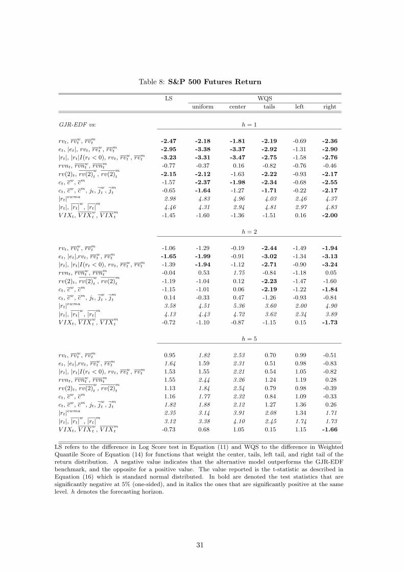
Table 8: S&P 500 Futures Return

LS WQS

uniform center tails left right

GJR-EDF vs: h = 1

rvt, rvwt , rvm

t -2.47 -2.18 -1.81 -2.19 -0.69 -2.36

et, |et|, rvt, rvwt , rvm

t -2.95 -3.38 -3.37 -2.92 -1.31 -2.90

|rt|, |rt|I(rt < 0), rvt, rvwt , rvm

t -3.23 -3.31 -3.47 -2.75 -1.58 -2.76

rvnt, rvnwt , rvnm

t -0.77 -0.37 0.16 -0.82 -0.76 -0.46

rv(2)t, rv(2)w

t , rv(2)m

t -2.15 -2.12 -1.63 -2.22 -0.93 -2.17

ct, cw, cm -1.57 -2.37 -1.98 -2.34 -0.68 -2.55

ct, cw, cm, jt, j

w

t , jm

t -0.65 -1.64 -1.27 -1.71 -0.22 -2.17

|rt|ewma 2.98 4.83 4.96 4.03 2.46 4.37

|rt|, |rt|w

, |rt|m

4.46 4.31 2.94 4.81 2.97 4.83

V IXt, V IXwt , V IX

mt -1.45 -1.60 -1.36 -1.51 0.16 -2.00

h = 2

rvt, rvwt , rvm

t -1.06 -1.29 -0.19 -2.44 -1.49 -1.94

et, |et|,rvt, rvwt , rvm

t -1.65 -1.99 -0.91 -3.02 -1.34 -3.13

|rt|, |rt|I(rt < 0), rvt, rvwt , rvm

t -1.39 -1.94 -1.12 -2.71 -0.90 -3.24

rvnt, rvnwt , rvnm

t -0.04 0.53 1.75 -0.84 -1.18 0.05

rv(2)t, rv(2)w

t , rv(2)m

t -1.19 -1.04 0.12 -2.23 -1.47 -1.60

ct, cw, cm -1.15 -1.01 0.06 -2.19 -1.22 -1.84

ct, cw, cm, jt, j

w

t , jm

t 0.14 -0.33 0.47 -1.26 -0.93 -0.84

|rt|ewma 3.58 4.51 5.36 3.60 2.00 4.90

|rt|, |rt|w

, |rt|m

4.13 4.43 4.72 3.62 2.34 3.89

V IXt, V IXwt , V IX

mt -0.72 -1.10 -0.87 -1.15 0.15 -1.73

h = 5

rvt, rvwt , rvm

t 0.95 1.82 2.53 0.70 0.99 -0.51

et, |et|,rvt, rvwt , rvm

t 1.64 1.59 2.31 0.51 0.98 -0.83

|rt|, |rt|I(rt < 0), rvt, rvwt , rvm

t 1.53 1.55 2.21 0.54 1.05 -0.82

rvnt, rvnwt , rvnm

t 1.55 2.44 3.26 1.24 1.19 0.28

rv(2)t, rv(2)w

t , rv(2)m

t 1.13 1.84 2.54 0.79 0.98 -0.39

ct, cw, cm 1.16 1.77 2.32 0.84 1.09 -0.33

ct, cw, cm, jt, j

w

t , jm

t 1.82 1.88 2.12 1.27 1.36 0.26

|rt|ewma 2.35 3.14 3.91 2.08 1.34 1.71

|rt|, |rt|w

, |rt|m

3.12 3.38 4.10 2.45 1.74 1.73

V IXt, V IXwt , V IX

mt -0.73 0.68 1.05 0.15 1.15 -1.66

LS refers to the difference in Log Score test in Equation (11) and WQS to the difference in WeightedQuantile Score of Equation (14) for functions that weight the center, tails, left tail, and right tail of thereturn distribution. A negative value indicates that the alternative model outperforms the GJR-EDFbenchmark, and the opposite for a positive value. The value reported is the t-statistic as described inEquation (16) which is standard normal distributed. In bold are denoted the test statistics that aresignificantly negative at 5% (one-sided), and in italics the ones that are significantly positive at the samelevel. h denotes the forecasting horizon.

31

Table 9: S&P 500 Futures Return

QS(τ)

0.01 0.05 0.10 0.20 0.30 0.40 0.60 0.70 0.80 0.90 0.95 0.99

GJR-EDF vs: h = 1

rvt, rvwt , rvm

t 0.44 -1.01 -1.07 -0.96 -1.27 0.53 -0.28 -1.47 -1.98 -2.40 -2.23 -0.93

et, |et|, rvt, rvwt , rvm

t 0.32 -1.19 -1.57 -2.02 -2.74 -1.31 -1.21 -2.21 -2.69 -2.86 -2.56 -1.19

|rt|, |rt|I(rt < 0), rvt, rvwt , rvm

t -0.06 -1.26 -1.39 -2.21 -2.69 -1.53 -1.36 -2.79 -3.03 -2.71 -2.32 -0.82

rvnt, rvnwt , rvnm

t -1.80 0.16 -0.27 -0.69 -1.14 0.54 0.69 0.78 0.34 -0.83 -0.88 0.24

rv(2)t, rv(2)w

t , rv(2)m

t 0.17 -1.13 -1.48 -0.79 -1.61 0.21 0.06 -0.79 -1.64 -1.92 -2.22 -1.39

ct, cw, cm 0.03 -0.77 -0.85 -0.60 -1.15 0.34 -0.13 -1.80 -2.36 -2.55 -2.19 -1.03

ct, cw, cm, jt, j

w

t , jm

t 0.48 -0.45 -0.74 -0.35 -0.35 1.29 -0.17 -1.65 -1.82 -2.24 -2.08 -0.52

|rt|ewma 1.15 2.48 2.71 2.25 0.78 -0.19 2.68 4.92 5.05 3.92 3.83 2.14

|rt|, |rt|w

, |rt|m

1.90 3.44 2.67 0.78 -0.03 -0.84 2.06 4.55 4.78 3.94 3.63 2.63

V IXt, V IXwt , V IX

mt -0.54 -0.03 0.65 0.52 0.50 0.79 -1.09 -2.34 -2.40 -1.82 -1.71 -0.76

h = 2

rvt, rvwt , rvm

t -2.16 -1.60 -0.93 -0.71 1.38 2.73 -0.21 -1.44 -1.44 -1.34 -1.67 -1.68

et, |et|,rvt, rvwt , rvm

t -2.04 -1.50 -0.74 -0.64 1.23 2.80 -0.98 -2.50 -2.35 -2.33 -2.60 -2.34

|rt|, |rt|I(rt < 0), rvt, rvwt , rvm

t -1.10 -1.23 -0.50 -0.56 0.84 2.37 -1.35 -2.53 -2.53 -2.35 -2.68 -2.75

rvnt, rvnwt , rvnm

t -1.72 -1.26 -0.69 -0.37 2.01 2.69 1.53 0.37 0.74 0.38 -0.36 -0.75

rv(2)t, rv(2)w

t , rv(2)m

t -2.29 -1.50 -0.99 -0.59 1.25 2.49 0.33 -1.03 -1.09 -0.98 -1.57 -1.36

ct, cw, cm -1.68 -1.58 -0.91 0.02 1.92 2.63 -0.52 -1.57 -1.39 -1.04 -1.50 -1.81

ct, cw, cm, jt, j

w

t , jm

t -1.35 -1.03 -0.69 -0.03 1.67 2.74 0.12 -0.97 -1.02 -0.78 -0.59 -0.18

|rt|ewma 0.95 2.05 2.16 1.74 1.50 2.44 3.00 4.64 4.18 4.96 3.78 1.16

|rt|, |rt|w

, |rt|m

1.03 2.28 3.12 2.74 1.40 2.17 3.13 3.19 4.12 4.07 2.72 0.88

V IXt, V IXwt , V IX

mt -0.61 -0.13 0.91 0.23 0.76 2.19 -1.14 -2.68 -2.10 -1.83 -1.78 0.52

h = 5

rvt, rvwt , rvm

t 0.55 0.66 0.88 1.73 2.75 3.58 1.71 1.08 0.76 0.06 -1.34 -1.14

et, |et|,rvt, rvwt , rvm

t 0.50 0.68 0.82 1.73 2.94 3.69 1.30 0.42 0.28 -0.42 -1.44 -1.03

|rt|, |rt|I(rt < 0), rvt, rvwt , rvm

t 0.61 0.70 0.88 1.79 2.71 3.77 1.40 0.09 0.00 -0.31 -1.46 -0.88

rvnt, rvnwt , rvnm

t 0.64 0.92 1.16 1.92 2.80 3.95 2.48 1.56 1.32 0.68 -0.48 -0.62

rv(2)t, rv(2)w

t , rv(2)m

t 0.57 0.71 1.00 1.73 2.53 3.40 1.86 1.18 1.12 -0.05 -1.16 -1.24

ct, cw, cm 0.65 0.70 1.01 1.88 2.67 3.27 1.56 0.66 0.46 0.10 -1.11 -0.36

ct, cw, cm, jt, j

w

t , jm

t 0.74 1.16 1.18 2.01 2.59 2.84 1.31 0.81 0.81 0.51 -0.60 0.41

|rt|ewma 1.29 1.09 0.90 1.83 2.58 2.98 2.83 2.15 2.17 1.70 0.98 1.25

|rt|, |rt|w

, |rt|m

1.31 1.53 1.63 2.27 2.84 3.50 2.87 1.99 2.12 1.68 0.88 1.57

V IXt, V IXwt , V IX

mt 0.91 0.81 0.98 1.72 2.30 2.84 0.53 -1.02 -1.56 -1.43 -1.94 -0.77

QS(τ) refers to the difference in Quantile Score test at level τ (ranging from 0.01 to 0.99) discussed in Equation (13).A negative value indicates that the alternative model outperforms the GJR-EDF benchmark, and the opposite for apositive value. The value reported is the t-statistic as described in Equation (16) which is standard normal distributed.In bold are denoted the test statistics that are significantly negative at 5% (one-sided), and in italics the ones that aresignificantly positive at the same level. h denotes the forecasting horizon.

32

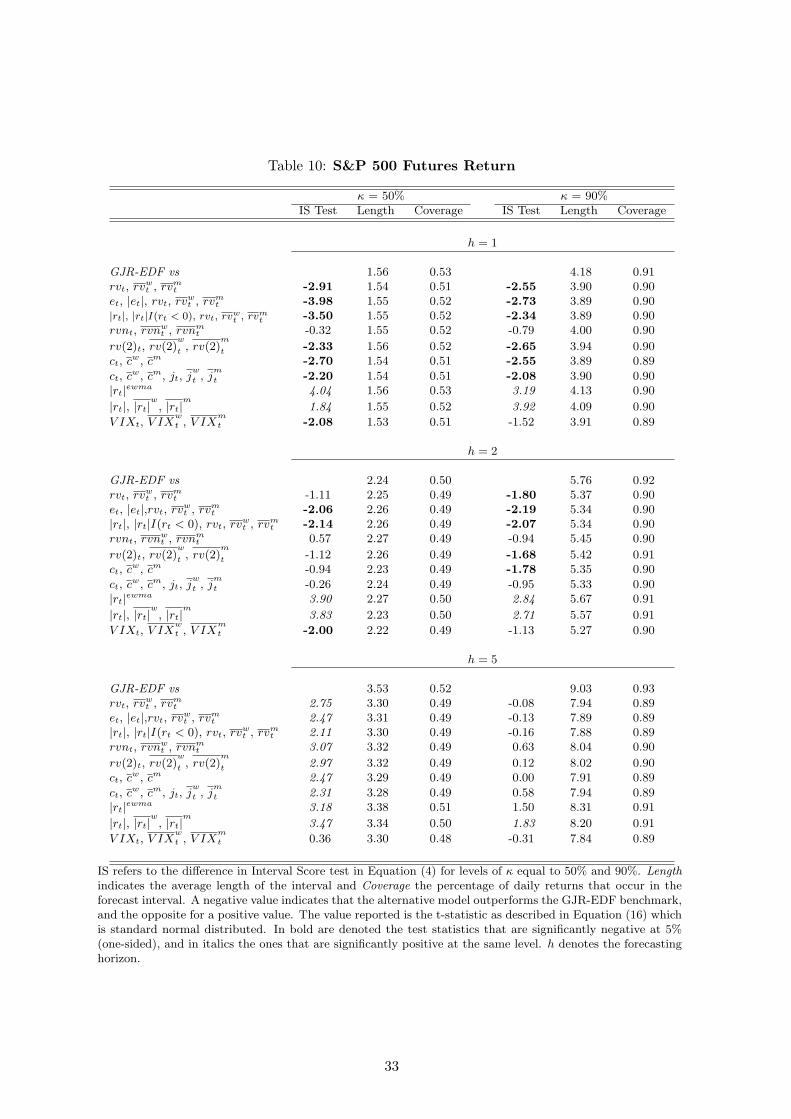
Table 10: S&P 500 Futures Return

κ = 50% κ = 90%IS Test Length Coverage IS Test Length Coverage

h = 1

GJR-EDF vs 1.56 0.53 4.18 0.91rvt, rv

wt , rvm

t -2.91 1.54 0.51 -2.55 3.90 0.90et, |et|, rvt, rv

wt , rvm

t -3.98 1.55 0.52 -2.73 3.89 0.90|rt|, |rt|I(rt < 0), rvt, rvw

t , rvmt -3.50 1.55 0.52 -2.34 3.89 0.90

rvnt, rvnwt , rvnm

t -0.32 1.55 0.52 -0.79 4.00 0.90

rv(2)t, rv(2)w

t , rv(2)m

t -2.33 1.56 0.52 -2.65 3.94 0.90ct, c

w, cm -2.70 1.54 0.51 -2.55 3.89 0.89

ct, cw, cm, jt, j

w

t , jm

t -2.20 1.54 0.51 -2.08 3.90 0.90|rt|ewma 4.04 1.56 0.53 3.19 4.13 0.90

|rt|, |rt|w

, |rt|m

1.84 1.55 0.52 3.92 4.09 0.90

V IXt, V IXwt , V IX

mt -2.08 1.53 0.51 -1.52 3.91 0.89

h = 2

GJR-EDF vs 2.24 0.50 5.76 0.92rvt, rv

wt , rvm

t -1.11 2.25 0.49 -1.80 5.37 0.90et, |et|,rvt, rv

wt , rvm

t -2.06 2.26 0.49 -2.19 5.34 0.90|rt|, |rt|I(rt < 0), rvt, rv

wt , rvm

t -2.14 2.26 0.49 -2.07 5.34 0.90rvnt, rvn

wt , rvnm

t 0.57 2.27 0.49 -0.94 5.45 0.90

rv(2)t, rv(2)w

t , rv(2)m

t -1.12 2.26 0.49 -1.68 5.42 0.91ct, c

w, cm -0.94 2.23 0.49 -1.78 5.35 0.90

ct, cw, cm, jt, j

w

t , jm

t -0.26 2.24 0.49 -0.95 5.33 0.90|rt|ewma 3.90 2.27 0.50 2.84 5.67 0.91

|rt|, |rt|w

, |rt|m

3.83 2.23 0.50 2.71 5.57 0.91

V IXt, V IXwt , V IX

mt -2.00 2.22 0.49 -1.13 5.27 0.90

h = 5

GJR-EDF vs 3.53 0.52 9.03 0.93rvt, rv

wt , rvm

t 2.75 3.30 0.49 -0.08 7.94 0.89et, |et|,rvt, rv

wt , rvm

t 2.47 3.31 0.49 -0.13 7.89 0.89|rt|, |rt|I(rt < 0), rvt, rv

wt , rvm

t 2.11 3.30 0.49 -0.16 7.88 0.89rvnt, rvn

wt , rvnm

t 3.07 3.32 0.49 0.63 8.04 0.90

rv(2)t, rv(2)w

t , rv(2)m

t 2.97 3.32 0.49 0.12 8.02 0.90ct, c

w, cm 2.47 3.29 0.49 0.00 7.91 0.89

ct, cw, cm, jt, j

w

t , jm

t 2.31 3.28 0.49 0.58 7.94 0.89|rt|ewma 3.18 3.38 0.51 1.50 8.31 0.91

|rt|, |rt|w

, |rt|m

3.47 3.34 0.50 1.83 8.20 0.91

V IXt, V IXwt , V IX

mt 0.36 3.30 0.48 -0.31 7.84 0.89

IS refers to the difference in Interval Score test in Equation (4) for levels of κ equal to 50% and 90%. Lengthindicates the average length of the interval and Coverage the percentage of daily returns that occur in theforecast interval. A negative value indicates that the alternative model outperforms the GJR-EDF benchmark,and the opposite for a positive value. The value reported is the t-statistic as described in Equation (16) whichis standard normal distributed. In bold are denoted the test statistics that are significantly negative at 5%(one-sided), and in italics the ones that are significantly positive at the same level. h denotes the forecastinghorizon.

33

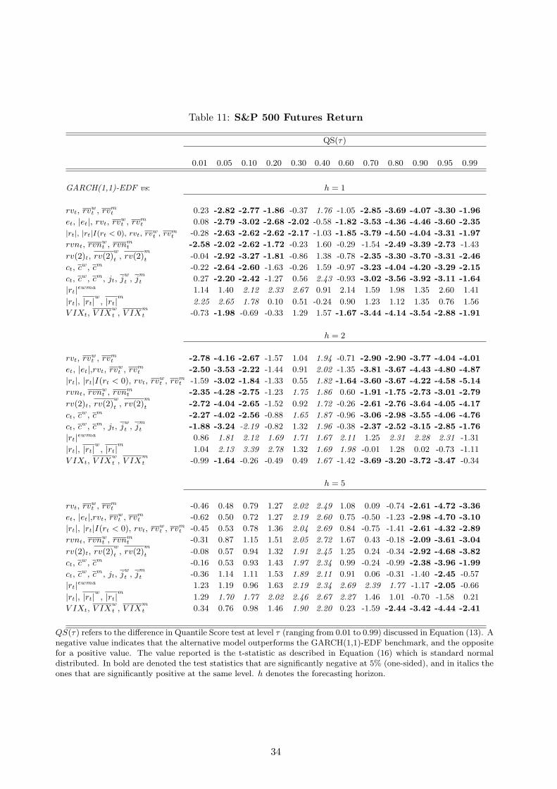
Table 11: S&P 500 Futures Return

QS(τ)

0.01 0.05 0.10 0.20 0.30 0.40 0.60 0.70 0.80 0.90 0.95 0.99

GARCH(1,1)-EDF vs: h = 1

rvt, rvwt , rvm

t 0.23 -2.82 -2.77 -1.86 -0.37 1.76 -1.05 -2.85 -3.69 -4.07 -3.30 -1.96

et, |et|, rvt, rvwt , rvm

t 0.08 -2.79 -3.02 -2.68 -2.02 -0.58 -1.82 -3.53 -4.36 -4.46 -3.60 -2.35

|rt|, |rt|I(rt < 0), rvt, rvwt , rvm

t -0.28 -2.63 -2.62 -2.62 -2.17 -1.03 -1.85 -3.79 -4.50 -4.04 -3.31 -1.97

rvnt, rvnwt , rvnm

t -2.58 -2.02 -2.62 -1.72 -0.23 1.60 -0.29 -1.54 -2.49 -3.39 -2.73 -1.43

rv(2)t, rv(2)w

t , rv(2)m

t -0.04 -2.92 -3.27 -1.81 -0.86 1.38 -0.78 -2.35 -3.30 -3.70 -3.31 -2.46

ct, cw, cm -0.22 -2.64 -2.60 -1.63 -0.26 1.59 -0.97 -3.23 -4.04 -4.20 -3.29 -2.15

ct, cw, cm, jt, j

w

t , jm

t 0.27 -2.20 -2.42 -1.27 0.56 2.43 -0.93 -3.02 -3.56 -3.92 -3.11 -1.64

|rt|ewma 1.14 1.40 2.12 2.33 2.67 0.91 2.14 1.59 1.98 1.35 2.60 1.41

|rt|, |rt|w

, |rt|m

2.25 2.65 1.78 0.10 0.51 -0.24 0.90 1.23 1.12 1.35 0.76 1.56

V IXt, V IXwt , V IX

mt -0.73 -1.98 -0.69 -0.33 1.29 1.57 -1.67 -3.44 -4.14 -3.54 -2.88 -1.91

h = 2

rvt, rvwt , rvm

t -2.78 -4.16 -2.67 -1.57 1.04 1.94 -0.71 -2.90 -2.90 -3.77 -4.04 -4.01

et, |et|,rvt, rvwt , rvm

t -2.50 -3.53 -2.22 -1.44 0.91 2.02 -1.35 -3.81 -3.67 -4.43 -4.80 -4.87

|rt|, |rt|I(rt < 0), rvt, rvwt , rvm

t -1.59 -3.02 -1.84 -1.33 0.55 1.82 -1.64 -3.60 -3.67 -4.22 -4.58 -5.14

rvnt, rvnwt , rvnm

t -2.35 -4.28 -2.75 -1.23 1.75 1.86 0.60 -1.91 -1.75 -2.73 -3.01 -2.79

rv(2)t, rv(2)w

t , rv(2)m

t -2.72 -4.04 -2.65 -1.52 0.92 1.72 -0.26 -2.61 -2.76 -3.64 -4.05 -4.17

ct, cw, cm -2.27 -4.02 -2.56 -0.88 1.65 1.87 -0.96 -3.06 -2.98 -3.55 -4.06 -4.76

ct, cw, cm, jt, j

w

t , jm

t -1.88 -3.24 -2.19 -0.82 1.32 1.96 -0.38 -2.37 -2.52 -3.15 -2.85 -1.76

|rt|ewma 0.86 1.81 2.12 1.69 1.71 1.67 2.11 1.25 2.31 2.28 2.31 -1.31

|rt|, |rt|w

, |rt|m

1.04 2.13 3.39 2.78 1.32 1.69 1.98 -0.01 1.28 0.02 -0.73 -1.11

V IXt, V IXwt , V IX

mt -0.99 -1.64 -0.26 -0.49 0.49 1.67 -1.42 -3.69 -3.20 -3.72 -3.47 -0.34

h = 5

rvt, rvwt , rvm

t -0.46 0.48 0.79 1.27 2.02 2.49 1.08 0.09 -0.74 -2.61 -4.72 -3.36

et, |et|,rvt, rvwt , rvm

t -0.62 0.50 0.72 1.27 2.19 2.60 0.75 -0.50 -1.23 -2.98 -4.70 -3.10

|rt|, |rt|I(rt < 0), rvt, rvwt , rvm

t -0.45 0.53 0.78 1.36 2.04 2.69 0.84 -0.75 -1.41 -2.61 -4.32 -2.89

rvnt, rvnwt , rvnm

t -0.31 0.87 1.15 1.51 2.05 2.72 1.67 0.43 -0.18 -2.09 -3.61 -3.04

rv(2)t, rv(2)w

t , rv(2)m

t -0.08 0.57 0.94 1.32 1.91 2.45 1.25 0.24 -0.34 -2.92 -4.68 -3.82

ct, cw, cm -0.16 0.53 0.93 1.43 1.97 2.34 0.99 -0.24 -0.99 -2.38 -3.96 -1.99

ct, cw, cm, jt, j

w

t , jm

t -0.36 1.14 1.11 1.53 1.89 2.11 0.91 0.06 -0.31 -1.40 -2.45 -0.57

|rt|ewma 1.23 1.19 0.96 1.63 2.19 2.34 2.69 2.39 1.77 -1.17 -2.05 -0.66

|rt|, |rt|w

, |rt|m

1.29 1.70 1.77 2.02 2.46 2.67 2.27 1.46 1.01 -0.70 -1.58 0.21

V IXt, V IXwt , V IX

mt 0.34 0.76 0.98 1.46 1.90 2.20 0.23 -1.59 -2.44 -3.42 -4.44 -2.41

QS(τ) refers to the difference in Quantile Score test at level τ (ranging from 0.01 to 0.99) discussed in Equation (13). Anegative value indicates that the alternative model outperforms the GARCH(1,1)-EDF benchmark, and the oppositefor a positive value. The value reported is the t-statistic as described in Equation (16) which is standard normaldistributed. In bold are denoted the test statistics that are significantly negative at 5% (one-sided), and in italics theones that are significantly positive at the same level. h denotes the forecasting horizon.

34

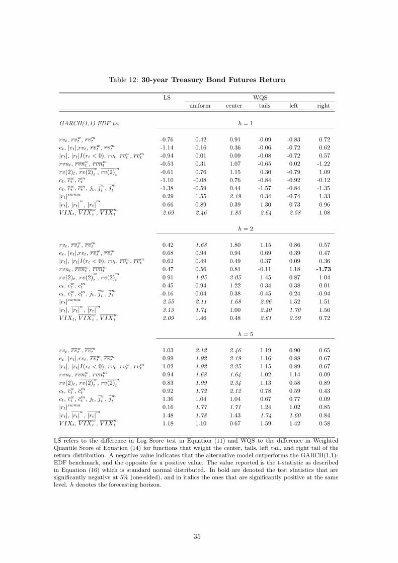
Table 12: 30-year Treasury Bond Futures Return

LS WQS

uniform center tails left right

GARCH(1,1)-EDF vs: h = 1

rvt, rvwt , rvm

t -0.76 0.42 0.91 -0.09 -0.83 0.72

et, |et|,rvt, rvwt , rvm

t -1.14 0.16 0.36 -0.06 -0.72 0.62

|rt|, |rt|I(rt < 0), rvt, rvwt , rvm

t -0.94 0.01 0.09 -0.08 -0.72 0.57

rvnt, rvnwt , rvnm

t -0.53 0.31 1.07 -0.65 0.02 -1.22

rv(2)t, rv(2)w

t , rv(2)m

t -0.61 0.76 1.15 0.30 -0.79 1.09

ct, cwt , cmt -1.10 -0.08 0.76 -0.84 -0.92 -0.12

ct, cwt , cmt , jt, j

w

t , jm

t -1.38 -0.59 0.44 -1.57 -0.84 -1.35

|rt|ewma 0.29 1.55 2.19 0.34 -0.74 1.33

|rt|, |rt|w

, |rt|m

0.66 0.89 0.39 1.30 0.73 0.96

V IXt, V IXwt , V IX

mt 2.69 2.46 1.83 2.64 2.58 1.08

h = 2

rvt, rvwt , rvm

t 0.42 1.68 1.80 1.15 0.86 0.57

et, |et|,rvt, rvwt , rvm

t 0.68 0.94 0.94 0.69 0.39 0.47

|rt|, |rt|I(rt < 0), rvt, rvwt , rvm

t 0.62 0.49 0.49 0.37 0.09 0.36

rvnt, rvnwt , rvnm

t 0.47 0.56 0.81 -0.11 1.18 -1.73

rv(2)t, rv(2)w

t , rv(2)m

t 0.91 1.95 2.05 1.45 0.87 1.04

ct, cwt , cmt -0.45 0.94 1.22 0.34 0.38 0.01

ct, cwt , cmt , jt, j

w

t , jm

t -0.16 0.04 0.38 -0.45 0.24 -0.94

|rt|ewma 2.55 2.11 1.68 2.06 1.52 1.51

|rt|, |rt|w

, |rt|m

3.13 1.74 1.00 2.40 1.70 1.56

V IXt, V IXwt , V IX

mt 2.09 1.46 0.48 2.61 2.59 0.72

h = 5

rvt, rvwt , rvm

t 1.03 2.12 2.46 1.19 0.90 0.65

et, |et|,rvt, rvwt , rvm

t 0.99 1.92 2.19 1.16 0.88 0.67

|rt|, |rt|I(rt < 0), rvt, rvwt , rvm

t 1.02 1.92 2.25 1.15 0.89 0.67

rvnt, rvnwt , rvnm

t 0.94 1.68 1.64 1.02 1.14 0.09

rv(2)t, rv(2)w

t , rv(2)m

t 0.83 1.99 2.34 1.13 0.58 0.89

ct, cwt , cmt 0.92 1.72 2.12 0.78 0.59 0.43

ct, cwt , cmt , jt, j

w

t , jm

t 1.36 1.04 1.04 0.67 0.77 0.09

|rt|ewma 0.16 1.77 1.71 1.24 1.02 0.85

|rt|, |rt|w

, |rt|m

1.48 1.78 1.43 1.74 1.60 0.84

V IXt, V IXwt , V IX

mt 1.18 1.10 0.67 1.59 1.42 0.58

LS refers to the difference in Log Score test in Equation (11) and WQS to the difference in WeightedQuantile Score of Equation (14) for functions that weight the center, tails, left tail, and right tail of thereturn distribution. A negative value indicates that the alternative model outperforms the GARCH(1,1)-EDF benchmark, and the opposite for a positive value. The value reported is the t-statistic as describedin Equation (16) which is standard normal distributed. In bold are denoted the test statistics that aresignificantly negative at 5% (one-sided), and in italics the ones that are significantly positive at the samelevel. h denotes the forecasting horizon.

35

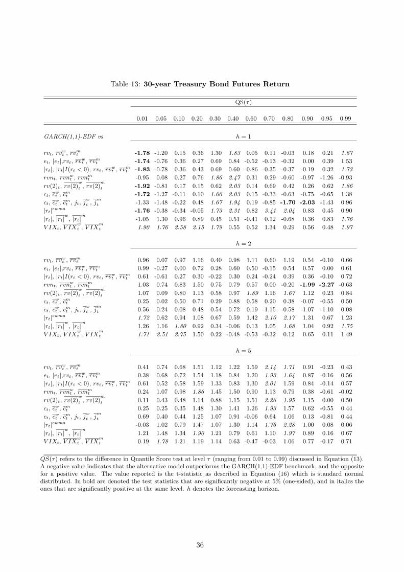
Table 13: 30-year Treasury Bond Futures Return

QS(τ)

0.01 0.05 0.10 0.20 0.30 0.40 0.60 0.70 0.80 0.90 0.95 0.99

GARCH(1,1)-EDF vs h = 1

rvt, rvwt , rvm

t -1.78 -1.20 0.15 0.36 1.30 1.83 0.05 0.11 -0.03 0.18 0.21 1.67

et, |et|,rvt, rvwt , rvm

t -1.74 -0.76 0.36 0.27 0.69 0.84 -0.52 -0.13 -0.32 0.00 0.39 1.53

|rt|, |rt|I(rt < 0), rvt, rvwt , rvm

t -1.83 -0.78 0.36 0.43 0.69 0.60 -0.86 -0.35 -0.37 -0.19 0.32 1.73

rvnt, rvnwt , rvnm

t -0.95 0.08 0.27 0.76 1.86 2.47 0.31 0.29 -0.60 -0.97 -1.26 -0.93

rv(2)t, rv(2)w

t , rv(2)m

t -1.92 -0.81 0.17 0.15 0.62 2.03 0.14 0.69 0.42 0.26 0.62 1.86

ct, cwt , cmt -1.72 -1.27 -0.11 0.10 1.66 2.03 0.15 -0.33 -0.63 -0.75 -0.65 1.38

ct, cwt , cmt , jt, j

w

t , jm

t -1.33 -1.48 -0.22 0.48 1.67 1.94 0.19 -0.85 -1.70 -2.03 -1.43 0.96

|rt|ewma -1.76 -0.38 -0.34 -0.05 1.73 2.31 0.82 3.41 2.04 0.83 0.45 0.90

|rt|, |rt|w

, |rt|m

-1.05 1.30 0.96 0.89 0.45 0.51 -0.41 0.12 -0.68 0.36 0.83 1.76

V IXt, V IXwt , V IX

mt 1.90 1.76 2.58 2.15 1.79 0.55 0.52 1.34 0.29 0.56 0.48 1.97

h = 2

rvt, rvwt , rvm

t 0.96 0.07 0.97 1.16 0.40 0.98 1.11 0.60 1.19 0.54 -0.10 0.66

et, |et|,rvt, rvwt , rvm

t 0.99 -0.27 0.00 0.72 0.28 0.60 0.50 -0.15 0.54 0.57 0.00 0.61

|rt|, |rt|I(rt < 0), rvt, rvwt , rvm

t 0.61 -0.61 0.27 0.30 -0.22 0.30 0.24 -0.24 0.39 0.36 -0.10 0.72

rvnt, rvnwt , rvnm

t 1.03 0.74 0.83 1.50 0.75 0.79 0.57 0.00 -0.20 -1.99 -2.27 -0.63

rv(2)t, rv(2)w

t , rv(2)m

t 1.07 0.09 0.80 1.13 0.58 0.97 1.89 1.16 1.67 1.12 0.23 0.84

ct, cwt , cmt 0.25 0.02 0.50 0.71 0.29 0.88 0.58 0.20 0.38 -0.07 -0.55 0.50

ct, cwt , cmt , jt, j

w

t , jm

t 0.56 -0.24 0.08 0.48 0.54 0.72 0.19 -1.15 -0.58 -1.07 -1.10 0.08

|rt|ewma 1.72 0.62 0.94 1.08 0.67 0.59 1.42 2.10 2.17 1.31 0.67 1.23

|rt|, |rt|w

, |rt|m

1.26 1.16 1.80 0.92 0.34 -0.06 0.13 1.05 1.68 1.04 0.92 1.75

V IXt, V IXwt , V IX

mt 1.71 2.51 2.75 1.50 0.22 -0.48 -0.53 -0.32 0.12 0.65 0.11 1.49

h = 5

rvt, rvwt , rvm

t 0.41 0.74 0.68 1.51 1.12 1.22 1.59 2.14 1.71 0.91 -0.23 0.43

et, |et|,rvt, rvwt , rvm

t 0.38 0.68 0.72 1.54 1.18 0.84 1.20 1.93 1.64 0.87 -0.16 0.56

|rt|, |rt|I(rt < 0), rvt, rvwt , rvm

t 0.61 0.52 0.58 1.59 1.33 0.83 1.30 2.01 1.59 0.84 -0.14 0.57

rvnt, rvnwt , rvnm

t 0.24 1.07 0.98 1.86 1.45 1.50 0.90 1.13 0.79 0.38 -0.61 -0.02

rv(2)t, rv(2)w

t , rv(2)m

t 0.11 0.43 0.48 1.14 0.88 1.15 1.51 2.26 1.95 1.15 0.00 0.50

ct, cwt , cmt 0.25 0.25 0.35 1.48 1.30 1.41 1.26 1.93 1.57 0.62 -0.55 0.44

ct, cwt , cmt , jt, j

w

t , jm

t 0.69 0.40 0.44 1.25 1.07 0.91 -0.06 0.64 1.06 0.13 -0.81 0.44

|rt|ewma -0.03 1.02 0.79 1.47 1.07 1.30 1.14 1.76 2.28 1.00 0.08 0.06

|rt|, |rt|w

, |rt|m

1.21 1.48 1.34 1.90 1.21 0.79 0.61 1.10 1.97 0.89 0.16 0.67

V IXt, V IXwt , V IX

mt 0.19 1.78 1.21 1.19 1.14 0.63 -0.47 -0.03 1.06 0.77 -0.17 0.71

QS(τ) refers to the difference in Quantile Score test at level τ (ranging from 0.01 to 0.99) discussed in Equation (13).A negative value indicates that the alternative model outperforms the GARCH(1,1)-EDF benchmark, and the oppositefor a positive value. The value reported is the t-statistic as described in Equation (16) which is standard normaldistributed. In bold are denoted the test statistics that are significantly negative at 5% (one-sided), and in italics theones that are significantly positive at the same level. h denotes the forecasting horizon.

36

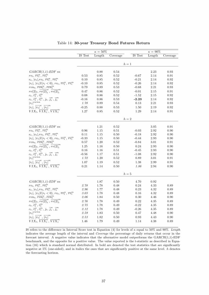
Table 14: 30-year Treasury Bond Futures Return

κ = 50% κ = 90%IS Test Length Coverage IS Test Length Coverage

h = 1

GARCH(1,1)-EDF vs: 0.88 0.54 2.23 0.93rvt, rv

wt , rvm

t 0.53 0.85 0.52 -0.67 2.14 0.91et, |et|,rvt, rv

wt , rvm

t 0.10 0.85 0.52 -0.21 2.14 0.92|rt|, |rt|I(rt < 0), rvt, rv

wt , rvm

t -0.10 0.85 0.52 -0.26 2.14 0.92rvnt, rvn

wt , rvnm

t 0.79 0.89 0.53 -0.68 2.21 0.93

rv(2)t, rv(2)w

t , rv(2)m

t 0.47 0.86 0.52 -0.01 2.15 0.91ct, c

wt , cmt 0.08 0.86 0.52 -1.52 2.15 0.92

ct, cwt , cmt , jt, j

w

t , jm

t -0.16 0.86 0.53 -2.23 2.14 0.92|rt|ewma 1.78 0.89 0.54 0.13 2.21 0.93

|rt|, |rt|w

, |rt|m

-0.25 0.88 0.53 1.50 2.19 0.92

V IXt, V IXwt , V IX

mt 1.27 0.85 0.52 1.29 2.14 0.91

h = 2

GARCH(1,1)-EDF vs: 1.21 0.52 3.05 0.91rvt, rv

wt , rvm

t 0.96 1.15 0.51 -0.03 2.92 0.90et, |et|,rvt, rv

wt , rvm

t 0.11 1.15 0.50 -0.18 2.92 0.90|rt|, |rt|I(rt < 0), rvt, rv

wt , rvm

t -0.33 1.15 0.50 -0.44 2.93 0.90rvnt, rvn

wt , rvnm

t 0.57 1.20 0.52 -0.84 3.01 0.91

rv(2)t, rv(2)w

t , rv(2)m

t 1.25 1.16 0.50 0.24 2.93 0.90ct, c

wt , cmt 0.16 1.16 0.51 -0.45 2.93 0.90

ct, cwt , cmt , jt, j

w

t , jm

t -0.56 1.17 0.51 -1.08 2.92 0.90|rt|ewma 1.72 1.20 0.52 0.89 3.01 0.91

|rt|, |rt|w

, |rt|m

1.07 1.19 0.52 1.38 2.99 0.91

V IXt, V IXwt , V IX

mt 0.21 1.14 0.50 1.86 2.94 0.90

h = 5

GARCH(1,1)-EDF vs: 1.87 0.50 4.70 0.92rvt, rv

wt , rvm

t 2.78 1.78 0.48 0.24 4.33 0.89et, |et|,rvt, rv

wt , rvm

t 2.96 1.77 0.48 0.23 4.32 0.89|rt|, |rt|I(rt < 0), rvt, rv

wt , rvm

t 3.03 1.78 0.48 0.16 4.32 0.89rvnt, rvn

wt , rvnm

t 2.06 1.84 0.50 0.30 4.46 0.90

rv(2)t, rv(2)w

t , rv(2)m

t 2.76 1.78 0.49 0.22 4.35 0.89ct, c

wt , cmt 2.75 1.78 0.49 -0.22 4.35 0.89

ct, cwt , cmt , jt, j

w

t , jm

t 2.12 1.78 0.49 -0.26 4.35 0.89|rt|ewma 2.59 1.83 0.50 0.47 4.48 0.90

|rt|, |rt|w

, |rt|m

2.53 1.82 0.50 0.93 4.43 0.90

V IXt, V IXwt , V IX

mt 1.46 1.79 0.49 1.14 4.38 0.89

IS refers to the difference in Interval Score test in Equation (4) for levels of κ equal to 50% and 90%. Lengthindicates the average length of the interval and Coverage the percentage of daily returns that occur in theforecast interval. A negative value indicates that the alternative model outperforms the GARCH(1,1)-EDFbenchmark, and the opposite for a positive value. The value reported is the t-statistic as described in Equa-tion (16) which is standard normal distributed. In bold are denoted the test statistics that are significantlynegative at 5% (one-sided), and in italics the ones that are significantly positive at the same level. h denotesthe forecasting horizon.

37

05

10

15

IQR

2000 2002 2004 2006 2008 2010

GARCH(1,1)−EDF

05

10

15

IQR

2000 2002 2004 2006 2008 2010

GJR−EDF

05

10

15

IQR

2000 2002 2004 2006 2008 2010

rvt, rvt

w, rv

t

m

(a) Interquartile Range

05

10

15

20

25

95%

Inte

rval

2000 2002 2004 2006 2008 2010

GARCH(1,1)−EDF

05

10

15

20

25

95%

Inte

rval

2000 2002 2004 2006 2008 2010

GJR−EDF

05

10

15

20

25

95%

Inte

rval

2000 2002 2004 2006 2008 2010

rvt, rvt

w, rv

t

m

(b) 95% Interval

−0.2

−0.1

0.0

0.1

0.2

0.3

0.4

Skew

ne

ss

2000 2002 2004 2006 2008 2010

GARCH(1,1)−EDFGARCH(1,1)−EDF

−0.2

−0.1

0.0

0.1

0.2

0.3

0.4

Skew

ne

ss

2000 2002 2004 2006 2008 2010

GJR−EDFGJR−EDF

−0.2

−0.1

0.0

0.1

0.2

0.3

0.4

Skew

ne

ss

2000 2002 2004 2006 2008 2010

rvt, rvt

w, rv

t

mrvt, rvt

w, rv

t

m

(c) Skewness

−1.0

−0.5

0.0

0.5

1.0

1.5

2.0

Excess K

urt

osis

2000 2002 2004 2006 2008 2010

GARCH(1,1)−EDF

−1.0

−0.5

0.0

0.5

1.0

1.5

2.0

Excess K

urt

osis

2000 2002 2004 2006 2008 2010

GJR−EDF

−1.0

−0.5

0.0

0.5

1.0

1.5

2.0

Excess K

urt

osis

2000 2002 2004 2006 2008 2010

rvt, rvt

w, rv

t

m

(d) Kurtosis

Figure 2: Time series of the estimated IQRt,1, 95% interval forecast, SKt,1 and Kt,1 for theGARCH(1,1)-EDF (left column), GJR-EDF (center), and quantile model with regressors Xt =[rvt, rvwt , rv

mt ].

38

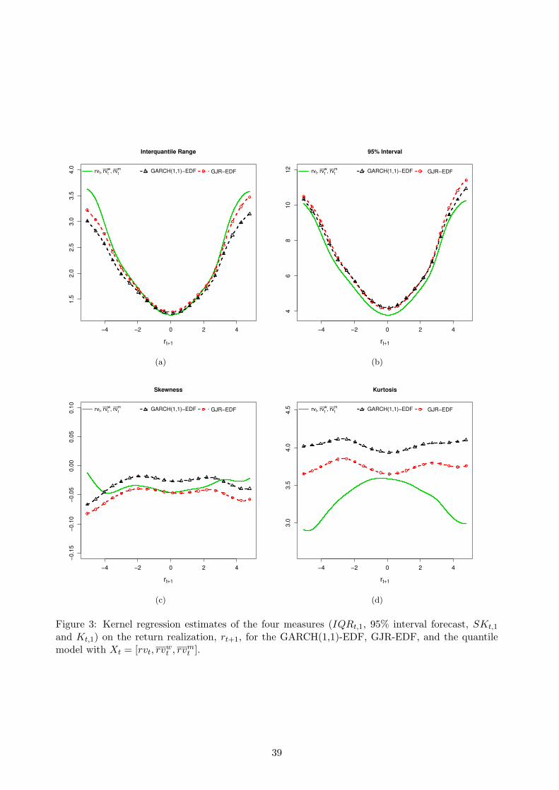
−4 −2 0 2 4

1.5

2.0

2.5

3.0

3.5

4.0

rt+1

rvt, rvtw, rvt

mGARCH(1,1)−EDF GJR−EDF

Interquantile Range

(a)

−4 −2 0 2 4

46

810

12

rt+1

rvt, rvtw, rvt

mGARCH(1,1)−EDF GJR−EDF

95% Interval

(b)

−4 −2 0 2 4

−0.1

5−

0.1

0−

0.0

50.0

00.0

50.1

0

rt+1

rvt, rvtw, rvt

mGARCH(1,1)−EDF GJR−EDF

Skewness

(c)

−4 −2 0 2 4

3.0

3.5

4.0

4.5

rt+1

rvt, rvtw, rvt

mGARCH(1,1)−EDF GJR−EDF

Kurtosis

(d)

Figure 3: Kernel regression estimates of the four measures (IQRt,1, 95% interval forecast, SKt,1

and Kt,1) on the return realization, rt+1, for the GARCH(1,1)-EDF, GJR-EDF, and the quantilemodel with Xt = [rvt, rvwt , rv

mt ].

39

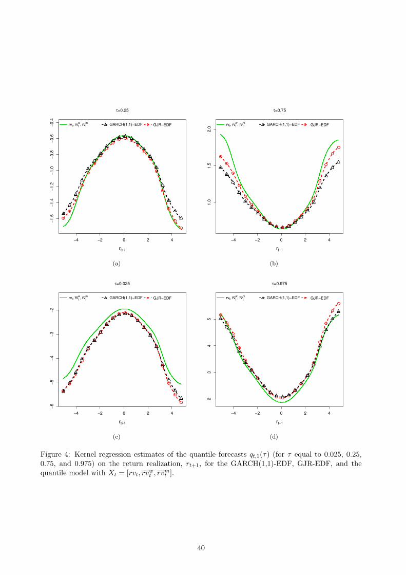
−4 −2 0 2 4

−1.6

−1.4

−1.2

−1.0

−0.8

−0.6

−0.4

rt+1

τ=0.25

rvt, rvtw, rvt

mGARCH(1,1)−EDF GJR−EDF

(a)

−4 −2 0 2 4

1.0

1.5

2.0

rt+1

τ=0.75

rvt, rvtw, rvt

mGARCH(1,1)−EDF GJR−EDF

(b)

−4 −2 0 2 4

−6

−5

−4

−3

−2

rt+1

τ=0.025

rvt, rvtw, rvt

mGARCH(1,1)−EDF GJR−EDF

(c)

−4 −2 0 2 4

23

45

rt+1

τ=0.975

rvt, rvtw, rvt

mGARCH(1,1)−EDF GJR−EDF

(d)

Figure 4: Kernel regression estimates of the quantile forecasts qt,1(τ) (for τ equal to 0.025, 0.25,0.75, and 0.975) on the return realization, rt+1, for the GARCH(1,1)-EDF, GJR-EDF, and thequantile model with Xt = [rvt, rvwt , rv

mt ].

40

−4 −2 0 2 4

1.0

1.5

2.0

2.5

3.0

3.5

4.0

rt+1

rt , rtw, rt

m GARCH(1,1)−EDF GJR−EDF

Interquantile Range

(a)

−4 −2 0 2 4

46

810

12

rt+1

rt , rtw

, rtm GARCH(1,1)−EDF GJR−EDF

95% Interval

(b)

−4 −2 0 2 4

−0.1

5−

0.1

0−

0.0

50.0

00.0

50.1

0

rt+1

rt , rtw, rt

m GARCH(1,1)−EDF GJR−EDF

Skewness

(c)

−4 −2 0 2 4

3.0

3.5

4.0

4.5

rt+1

rt , rtw

, rtm GARCH(1,1)−EDF GJR−EDF

Kurtosis

(d)

Figure 5: Kernel regression estimates of the four measures (IQRt,1, 95% interval forecast, SKt,1

and Kt,1) on the return realization, rt+1, for the GARCH(1,1)-EDF, GJR-EDF, and the quantilemodel with Xt = [|rt|, |rt|w, |rt|m].

41

−4 −2 0 2 4

−1.8

−1.6

−1.4

−1.2

−1.0

−0.8

−0.6

−0.4

rt+1

τ=0.25

rt , rtw, rt

m GARCH(1,1)−EDF GJR−EDF

(a)

−4 −2 0 2 4

0.8

1.0

1.2

1.4

1.6

1.8

rt+1

τ=0.75

rt , rtw

, rtm GARCH(1,1)−EDF GJR−EDF

(b)

−4 −2 0 2 4

−6

−5

−4

−3

−2

rt+1

τ=0.025

rt , rtw, rt

m GARCH(1,1)−EDF GJR−EDF

(c)

−4 −2 0 2 4

23

45

rt+1

τ=0.975

rt , rtw

, rtm GARCH(1,1)−EDF GJR−EDF

(d)

Figure 6: Kernel regression estimates of the quantile forecasts qt,1(τ) (for τ equal to 0.025, 0.25,0.75, and 0.975) on the return realization, rt+1, for the GARCH(1,1)-EDF, GJR-EDF, and thequantile model with Xt = [|r|t, |r|wt , |r|mt ].

42