Forecasting the Maintenance of Quasi-Linear Mesoscale Convective Systems

Forecasting the Maintenance of Quasi-Linear Mesoscale Convective Systems

MICHAEL C. CONIGLIO

Cooperative Institute for Mesoscale Meteorological Studies, University of Oklahoma, and NOAA/OAR/National Severe StormsLaboratory, Norman, Oklahoma

HAROLD E. BROOKS

NOAA/OAR/National Severe Storms Laboratory, Norman, Oklahoma

STEVEN J. WEISS AND STEPHEN F. CORFIDI

NOAA/Storm Prediction Center, Norman, Oklahoma

(Manuscript received 12 December 2005, in final form 12 September 2006)

ABSTRACT

The problem of forecasting the maintenance of mesoscale convective systems (MCSs) is investigatedthrough an examination of observed proximity soundings. Furthermore, environmental variables that arestatistically different between mature and weakening MCSs are input into a logistic regression procedure todevelop probabilistic guidance on MCS maintenance, focusing on warm-season quasi-linear systems thatpersist for several hours. Between the mature and weakening MCSs, shear vector magnitudes over verydeep layers are the best discriminators among hundreds of kinematic and thermodynamic variables. Ananalysis of the shear profiles reveals that the shear component perpendicular to MCS motion (usuallyparallel to the leading line) accounts for much of this difference in low levels and the shear componentparallel to MCS motion accounts for much of this difference in mid- to upper levels. The lapse rates overa significant portion of the convective cloud layer, the convective available potential energy, and thedeep-layer mean wind speed are also very good discriminators and collectively provide a high level ofdiscrimination between the mature and dissipation soundings as revealed by linear discriminant analysis.Probabilistic equations developed from these variables used with short-term numerical model output showutility in forecasting the transition of an MCS with a solid line of 50� dBZ echoes to a more disorganizedsystem with unsteady changes in structure and propagation. This study shows that empirical forecast toolsbased on environmental relationships still have the potential to provide forecasters with improved infor-mation on the qualitative characteristics of MCS structure and longevity. This is especially important sincethe current and near-term value added by explicit numerical forecasts of convection is still uncertain.

1. Introduction

Forecasting the details of mesoscale convective sys-tems (MCSs; Zipser 1982) continues to be a difficultproblem. Recent advances in numerical weather pre-diction models and computing power have allowed forexplicit real-time prediction of MCSs over the past fewyears (Done et al. 2004; Kain et al. 2005). While these

forecasts are promising, their utility and how to best usetheir capabilities in support of operations is unclear(Kain et al. 2005). Therefore, refining our knowledge ofthe interactions of MCSs with their environment re-mains central to advancing our near-term ability toforecast MCSs.

Predicting MCS maintenance is fraught with chal-lenges such as understanding how deep convection issustained through system–environment interactions(Weisman and Rotunno 2004; Parker and Johnson2004a,b; Coniglio et al. 2006a), how preexisting meso-scale features influence the systems (Fritsch and Forbes2001; Trier and Davis 2005), and how the system itselfcan alter the inflow environment and feed back to

Corresponding author address: Dr. Michael C. Coniglio, Na-tional Weather Center, NSSL/FRDD, 120 David L. Boren Blvd.,Norman, OK 73072.E-mail: [email protected]

556 W E A T H E R A N D F O R E C A S T I N G VOLUME 22

DOI: 10.1175/WAF1006.1

© 2007 American Meteorological Society

WAF1006

changes in the system structure and longevity (Parkerand Johnson 2004c; Fovell et al. 2005).

Evans and Doswell (2001) provide observational evi-dence that the strength of the mean wind (0–6 km) andits effects on cold pool development and MCS motionplay a role in sustaining long-lived forward-propagatingMCSs that produce damaging surface winds (derechos)through modifying the inflow of unstable air. They alsoshow that a wide range of convective available potentialenergy (CAPE) and vertical wind shear is found in theenvironments of derechos, likely reflecting the varietyof forcing mechanisms present in the spectrum ofcases.

Through the use of wind profiler observations andnumerical model output, Gale et al. (2002) examinenocturnal MCSs to determine predictors of their dissi-pation. Similar to Evans and Doswell (2001), they findthat changes in the MCS’s speed may control its dissi-pation through changes in low-level storm-relative in-flow. However, despite some indications that a decreas-ing low-level jet intensity and low-level equivalent po-tential temperature (�e), and its advection, can beuseful in some cases, they did not find robust predictorsof MCS dissipation.

An analysis of derecho proximity soundings inConiglio et al. (2004) shows that, as in Evans andDoswell (2001), CAPE and low-level wind shear varyconsiderably in derecho environments. Coniglio et al.(2004) also emphasizes that significant wind shear oftenexists in the mid- and upper levels in the preconvectiveenvironment. An emphasis of this work is that windshear over deeper layers than those considered in pastidealized modeling studies may be important for themaintenance of these systems. Stensrud et al. (2005)echo this result and suggest that this is especially truewhen the cold pool is very strong. This point may beparticularly important because observations from theBow Echoes and Mesoscale Convective Vortex (MCV)Experiment (BAMEX1) field campaign suggest thatcold pools often extend to 3–5 km above ground (Bryanet al. 2005), which is deeper than cold pools in idealizedsimulations of convective systems (Coniglio and Stens-rud 2001; Weisman and Rotunno 2004).

The goals of this work are to examine a large datasetof observed proximity soundings to identify predictorsof MCS dissipation and to improve our understandingof MCS environments. The ultimate goal is to developforecast tools that provide probabilistic guidance on the

maintenance of MCSs. The focus is on the 3–12-h timescale, which could benefit Day 1 Severe Weather Out-looks, Mesoscale Discussions, and the issuance of Se-vere Weather Watches at the Storm Prediction Center(SPC), and short-term forecasts issued by local Na-tional Weather Service forecast offices.

The approach is to use statistical techniques (de-scribed in section 2) to identify the best predictors ofMCS dissipation and use these predictors to develop anequation for the conditional probability of a strong,mature MCS. This study focuses on the robust systemsthat obtain a linear or curved leading line (which wewill hereafter refer to as “quasi-linear”) and tend toproduce severe weather. Furthermore, the intention isto focus on systems that are driven primarily by coldpool processes and not those in which the dynamics arecomplicated by the presence of larger-scale externalforcing (Fritsch and Forbes 2001; Trier and Davis2005). The best predictors of MCS dissipation are dis-cussed in section 3. Included in this section is a briefsummary of some recent ideas on the importance ofcold pool–deep shear environment interactions onMCS maintenance and how it relates to the currentfindings. Section 4 introduces the MCS probabilityequation and illustrates its potential utility. A summaryand final discussion are given in section 5.

2. Data gathering and processing

a. MCS proximity soundings

To develop a large dataset of MCS proximity sound-ings, MCSs are identified by examining composites ofbase radar reflectivity for the months of May–Augustduring the 7-yr period of 1998–2004. We follow theParker and Johnson (2000) description of MCSs andfocus our attention on the type that have a nearly con-tiguous quasi-linear or bowed leading edge of reflectiv-ity values of at least 35 dBZ at least 100 km in length.Although a 100-km-long collection of cells could beconsidered an MCS if it persists for 2–3 h (Cotton et al.1989), we only consider events that maintained this spa-tial configuration for at least five continuous hours tofocus on the longer-lived events. From a set of over 600MCSs of this type, we identified 269 events in which aradiosonde observation was taken within about 200 kmand 3 h of the leading edge of the MCS and displayedno obvious signs of contamination from convection. Inaddition, only those soundings that appeared to be inthe inflow environment are included in this tally. Weadd 79 derecho proximity soundings that were identi-fied using a similar procedure in Coniglio et al. (2004)

1 BAMEX was a field program designed to obtain high-densitykinematic and thermodynamic observations in and around bow-echo MCSs and mesoscale convective vortices (Davis et al. 2004).

JUNE 2007 C O N I G L I O E T A L . 557

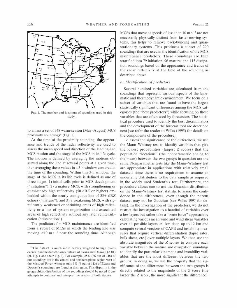
to amass a set of 348 warm-season (May–August) MCSproximity soundings2 (Fig. 1).

At the time of the proximity sounding, the appear-ance and trends of the radar reflectivity are used toassess the mean speed and direction of the leading-lineMCS motion and the stage of the MCS in its life cycle.The motion is defined by averaging the motions ob-served along the line at several points at a given time,then averaging these values in a 3-h window centered atthe time of the sounding. Within this 3-h window, thestage of the MCS in its life cycle is defined as one ofthree stages: 1) initial cells prior to MCS development(“initiation”); 2) a mature MCS, with strengthening orquasi-steady high reflectivity (50 dBZ or higher) em-bedded within the nearly contiguous line of 35� dBZechoes (“mature”); and 3) a weakening MCS, with sig-nificantly weakened or shrinking areas of high reflec-tivity or a loss of system organization and associatedareas of high reflectivity without any later reintensifi-cation (“dissipation”).

The predictors for MCS maintenance are identifiedfrom a subset of MCSs in which the leading line wasmoving �10 m s�1 near the sounding time. Although

MCSs that move at speeds of less than 10 m s�1 are notnecessarily physically distinct from faster-moving sys-tems, this helps to remove back-building and quasi-stationary systems. This produces a subset of 290soundings that are used in the identification of the MCSmaintenance predictors. These soundings are thenstratified into 79 initiation, 96 mature, and 115 dissipa-tion soundings based on the appearance and trends ofthe radar reflectivity at the time of the sounding asdescribed above.

b. Identification of predictors

Several hundred variables are calculated from thesoundings that represent various aspects of the kine-matic and thermodynamic environment. We focus on asubset of variables that are found to have the largeststatistically significant differences among the MCS cat-egories (the “best predictors”) while focusing on thosevariables that are often used by forecasters. The statis-tical procedure used to identify the best discriminatorsand the development of the forecast tool are describednext [we refer the reader to Wilks (1995) for details onthe components of the procedure].

To assess the significance of the differences, we usethe Mann–Whitney test to identify variables that givethe lowest probabilities (largest Z scores) that thepopulation “locations” (the nonparametric analog tothe mean) between the two groups in question are thesame. Nonparametric tests like the Mann–Whitney testare appropriate in applications with relatively smalldatasets since there is no requirement to assume anunderlying distribution to the data sample as requiredin the widely used Student’s t test. Furthermore, theprocedure allows one to use the Gaussian distributionon the Mann–Whitney test statistic to assess the confi-dence in the differences, even though the parentdataset may not be Gaussian (see Wilks 1995 for de-tails). In the investigation of the predictors, we do notrestrict the investigation to a handful of variables overa few layers but rather take a “brute force” approach bycalculating various mean wind and wind shear variablesover all possible layers �1 km deep up to 12 km andcompute several versions of CAPE and instability mea-sures that require vertical differentiation (lapse rates,bulk shear, etc.) over multiple layers. We then use theabsolute magnitude of the Z scores to compare eachvariable between the mature and dissipation soundingsto identify the particular kinematic and instability vari-ables that are the most different between the twogroups. In doing so, we use the property that the sig-nificance of the differences between the two groups isdirectly related to the magnitude of the Z score (thelarger the Z score, the more significant the difference).

2 This dataset is much more heavily weighted to high plainsevents than the derecho-only dataset of Evans and Doswell (2001)(cf. Fig. 1 and their Fig. 3). For example, 25% (86 out of 348) ofour soundings are in the central and northern plains region west ofthe Missouri River, whereas only 5% (6 out of 113) of Evans andDoswell’s soundings are found in this region. This disparity in thegeographical distribution of the soundings should be noted if oneattempts to compare and interpret the results of both studies.

FIG. 1. The number and locations of soundings used in thisstudy.


For example, a Z score of 1.96 (2.58) corresponds to a95% (99%) confidence that the “locations” of the twodistributions in space (or the mean in a parametric test)are different in a two-tailed hypothesis testing ap-proach.

Using the Z scores as a guide, linear discriminantanalyses are then used to find the number and particu-lar combination of variables that provide the best sepa-ration between the two groups in question. Thisamounts to determining the combination of variablesthat produces the highest percentage of correctlygrouped soundings in a discriminant analysis. As de-tailed later, we find that the percentage of correctgroupings converges to 1%–2% after the inclusion ofonly four variables in the analyses, which is a reflectionof the substantial mutual correlations among the vari-ables.

c. Logistic regression

Once the best predictors are identified, logistic re-gression3 is used to develop an equation that gives theprobability of one of the two groups occurring. Logisticregression is a method of producing probability fore-casts on a set of binary data (i.e., data within twogroups) by fitting predictors to the equation:

y �1

1 � exp�b0 � b1x1 � b2x2 � · · · � bkxk�, �1�

where the outputted y value is between one of the twobinary data values, k is the number of predictors, xk

refers to the kth predictor, and bk refers to the kthregression coefficient for each predictor. If the two in-put binary data values for the two groups are 0 and 1,then y becomes the fractional probability (0 � y � 1) ofone of the groups occurring. This explains why logisticregression is fitting in this context because the resultantpredictand is a probability; that is, it allows for the di-rect computation of probabilities between two possibleoutcomes in a set of data, which in this case is either amature or a dissipating MCS.

The logistic regression equation is designed primarilyto give the probability of a mature MCS as definedabove, conditional on the development of an MCS.However, a consequence of the experimental design isthat the predicted stage of the MCS is not independentof the predicted intensity of the MCS. This is becausemany of the same variables that discriminate well be-tween the mature and weakening stages of a particular

MCS also appear to discriminate well between MCSs ofdifferent intensities (Cohen et al. 2006). For example,large versus small CAPE could mean a mature versus aweakening MCS and a strong versus weak MCS. There-fore, the higher the probability of MCS maintenance,the more likely it is that an MCS will be maintained andbe strong in a given environment, but the relative con-tribution to MCS maintenance compared to MCS in-tensity cannot be determined solely from the predictorsin a particular case. We believe that this ambiguity ininterpretation, however, does not hinder the generalapplication of these ideas for the particular forecastproblem of MCS maintenance, as we will show next.

3. Best kinematic predictors

a. Mean wind shear

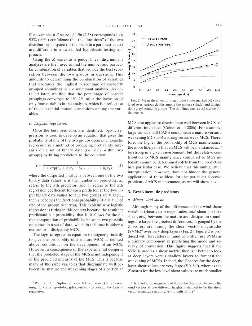
Although many of the differences of the wind shearvariables (shear vector magnitudes, total shear, positiveshear, etc.) between the mature and dissipation sound-ings are large, the greatest differences, as gauged by theZ scores, are among the shear vector magnitudes(SVMs)4 over very deep layers (Fig. 2). Figure 2 is pro-duced with forecasters in mind who often use SVMs asa primary component in predicting the mode and se-verity of convection. This figure suggests that if theSVM is used as a shear metric, then is it better to lookat deep layers versus shallow layers to forecast theweakening of MCSs. Indeed, the Z scores for the deep-layer shear values are very large (5.0–8.0), whereas theZ scores for the low-level shear values are much smaller

3 We used the S-plus, version 6.1, software (http://www.insightful.com/support/doc_splus_win.asp) to perform the logisticregression.

4 To clarify, the magnitude of the vector difference between thewind vectors at two different heights is defined to be the shearvector magnitude and is given in units of m s�1.

FIG. 2. Mean shear vector magnitudes (lines marked X) calcu-lated over various depths among the mature (black) and dissipa-tion (gray) sounding groups. The thin lines enclose �1 std dev forthe means.


(1.0–2.0) (not shown). In fact, the deep-layer SVMshave the largest Z scores of any variables tested. TheSVMs are larger for the mature soundings (Fig. 2) assuggested for derecho-producing MCSs alone (Coniglioet al. 2004). The differences in the low-level SVMs arerelatively small, suggesting that these values, alone,have limited utility in determining the stage of the MCSlife cycle.

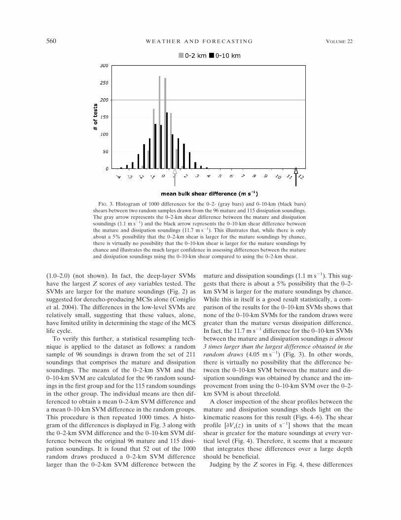
To verify this further, a statistical resampling tech-nique is applied to the dataset as follows: a randomsample of 96 soundings is drawn from the set of 211soundings that comprises the mature and dissipationsoundings. The means of the 0–2-km SVM and the0–10-km SVM are calculated for the 96 random sound-ings in the first group and for the 115 random soundingsin the other group. The individual means are then dif-ferenced to obtain a mean 0–2-km SVM difference anda mean 0–10-km SVM difference in the random groups.This procedure is then repeated 1000 times. A histo-gram of the differences is displayed in Fig. 3 along withthe 0–2-km SVM difference and the 0–10-km SVM dif-ference between the original 96 mature and 115 dissi-pation soundings. It is found that 52 out of the 1000random draws produced a 0–2-km SVM differencelarger than the 0–2-km SVM difference between the

mature and dissipation soundings (1.1 m s�1). This sug-gests that there is about a 5% possibility that the 0–2-km SVM is larger for the mature soundings by chance.While this in itself is a good result statistically, a com-parison of the results for the 0–10-km SVMs shows thatnone of the 0–10-km SVMs for the random draws weregreater than the mature versus dissipation difference.In fact, the 11.7 m s�1 difference for the 0–10-km SVMsbetween the mature and dissipation soundings is almost3 times larger than the largest difference obtained in therandom draws (4.05 m s�1) (Fig. 3). In other words,there is virtually no possibility that the difference be-tween the 0–10-km SVM between the mature and dis-sipation soundings was obtained by chance and the im-provement from using the 0–10-km SVM over the 0–2-km SVM is about threefold.

A closer inspection of the shear profiles between themature and dissipation soundings sheds light on thekinematic reasons for this result (Figs. 4–6). The shearprofile [Vs(z) in units of s�1] shows that the meanshear is greater for the mature soundings at every ver-tical level (Fig. 4). Therefore, it seems that a measurethat integrates these differences over a large depthshould be beneficial.

Judging by the Z scores in Fig. 4, these differences

FIG. 3. Histogram of 1000 differences for the 0–2- (gray bars) and 0–10-km (black bars)shears between two random samples drawn from the 96 mature and 115 dissipation soundings.The gray arrow represents the 0–2-km shear difference between the mature and dissipationsoundings (1.1 m s�1) and the black arrow represents the 0–10-km shear difference betweenthe mature and dissipation soundings (11.7 m s�1). This illustrates that, while there is onlyabout a 5% possibility that the 0–2-km shear is larger for the mature soundings by chance,there is virtually no possibility that the 0–10-km shear is larger for the mature soundings bychance and illustrates the much larger confidence in assessing differences between the matureand dissipation soundings using the 0–10-km shear compared to using the 0–2-km shear.


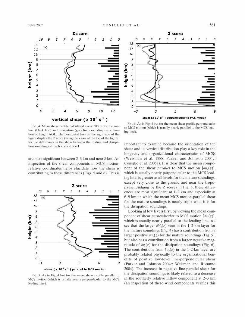
are most significant between 2–3 km and near 8 km. Aninspection of the shear components in MCS motion-relative coordinates helps elucidate how the shear iscontributing to these differences (Figs. 5 and 6). This is

important to examine because the orientation of theshear and its vertical distribution play a key role in thelongevity and organizational characteristics of MCSs(Weisman et al. 1988; Parker and Johnson 2004c;Coniglio et al. 2006a). It is clear that the mean compo-nent of the shear parallel to MCS motion [us(z)],which is usually nearly perpendicular to the MCS lead-ing line, is greater at all levels for the mature soundings,except very close to the ground and near the tropo-pause. Judging by the Z scores in Fig. 5, these differ-ences are most significant at 1–2 km and especially at6–9 km, in which the mean MCS motion-parallel shearfor the mature soundings is nearly triple what it is forthe dissipation soundings.

Looking at low levels first, by viewing the mean com-ponent of shear perpendicular to MCS motion [s(z)],which is usually nearly parallel to the leading line, wesee that the larger Vs(z) seen in the 1–2-km layer forthe mature soundings (Fig. 4) has a contribution from alarger positive us(z) for the mature soundings (Fig. 5),but also has a contribution from a larger negative mag-nitude of s(z) for the dissipation soundings (Fig. 6).The contributions from us(z) in the 1–2-km layer areprobably related physically to the organizational ben-efits of positive low-level line-perpendicular shear(Parker and Johnson 2004c; Weisman and Rotunno2004). The increase in negative line-parallel shear forthe dissipation soundings is likely related to a decreasein the southerly relative inflow component at 2–3 km(an inspection of these wind components verifies this

FIG. 4. Mean shear profile calculated every 500 m for the ma-ture (black line) and dissipation (gray line) soundings as a func-tion of height AGL. The horizontal bars on the right side of thefigure display the Z score (using the x axis at the top of the figure)for the differences in the shear between the mature and dissipa-tion soundings at each vertical level.

FIG. 5. As in Fig. 4 but for the mean shear profile parallel toMCS motion (which is usually nearly perpendicular to the MCSleading line).

FIG. 6. As in Fig. 4 but for the mean shear profile perpendicularto MCS motion (which is usually nearly parallel to the MCS lead-ing line).


claim). Collectively, Figs. 4–6 illustrate that the low-level SVMs represent differences in shear that are im-portant in both the line-perpendicular and line-paralleldirections.

Looking at the upper levels, the larger Vs(z) for themature soundings (Fig. 4) is much more apparent whenviewing the mean MCS motion-parallel shear (Fig. 5),in which the Z scores are �3 (corresponding to a �99%confidence in the statistical differences) for most levelsbetween 6 and 9 km. The larger shear is almost entirelydue to the larger us(z) (Fig. 5) since s(z) is nearlyidentical at 6–8 km between the two groups (Fig. 6).There are indications though that s(z) does becomeimportant above 8 km as the values become larger andnegative for the dissipation soundings. The most impor-tant point here though is that the possible physical ben-efits to mature MCSs related to a larger upper-levelshear component parallel to MCS motion are revealedin Fig. 5. Since this feature of MCS environments hasbeen given little attention in the literature compared tolow-level shear (Weisman and Rotunno 2004), webriefly review some recent ideas on how this upper-level line-normal shear can benefit mature MCSs.

1) COLD POOL–WIND SHEAR INTERACTIONS

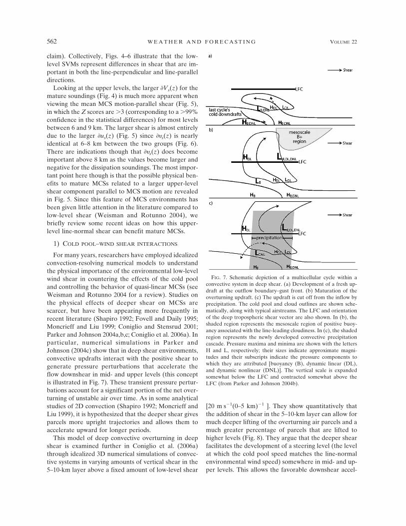
For many years, researchers have employed idealizedconvection-resolving numerical models to understandthe physical importance of the environmental low-levelwind shear in countering the effects of the cold pooland controlling the behavior of quasi-linear MCSs (seeWeisman and Rotunno 2004 for a review). Studies onthe physical effects of deeper shear on MCSs arescarcer, but have been appearing more frequently inrecent literature (Shapiro 1992; Fovell and Daily 1995;Moncrieff and Liu 1999; Coniglio and Stensrud 2001;Parker and Johnson 2004a,b,c; Coniglio et al. 2006a). Inparticular, numerical simulations in Parker andJohnson (2004c) show that in deep shear environments,convective updrafts interact with the positive shear togenerate pressure perturbations that accelerate theflow downshear in mid- and upper levels (this conceptis illustrated in Fig. 7). These transient pressure pertur-bations account for a significant portion of the net over-turning of unstable air over time. As in some analyticalstudies of 2D convection (Shapiro 1992; Moncrieff andLiu 1999), it is hypothesized that the deeper shear givesparcels more upright trajectories and allows them toaccelerate upward for longer periods.

This model of deep convective overturning in deepshear is examined further in Coniglio et al. (2006a)through idealized 3D numerical simulations of convec-tive systems in varying amounts of vertical shear in the5–10-km layer above a fixed amount of low-level shear

[20 m s�1(0–5 km)�1 ]. They show quantitatively thatthe addition of shear in the 5–10-km layer can allow formuch deeper lifting of the overturning air parcels and amuch greater percentage of parcels that are lifted tohigher levels (Fig. 8). They argue that the deeper shearfacilitates the development of a steering level (the levelat which the cold pool speed matches the line-normalenvironmental wind speed) somewhere in mid- and up-per levels. This allows the favorable downshear accel-

FIG. 7. Schematic depiction of a multicellular cycle within aconvective system in deep shear. (a) Development of a fresh up-draft at the outflow boundary–gust front. (b) Maturation of theoverturning updraft. (c) The updraft is cut off from the inflow byprecipitation. The cold pool and cloud outlines are shown sche-matically, along with typical airstreams. The LFC and orientationof the deep tropospheric shear vector are also shown. In (b), theshaded region represents the mesoscale region of positive buoy-ancy associated with the line-leading cloudiness. In (c), the shadedregion represents the newly developed convective precipitationcascade. Pressure maxima and minima are shown with the lettersH and L, respectively; their sizes indicate approximate magni-tudes and their subscripts indicate the pressure components towhich they are attributed [buoyancy (B), dynamic linear (DL),and dynamic nonlinear (DNL)]. The vertical scale is expandedsomewhat below the LFC and contracted somewhat above theLFC (from Parker and Johnson 2004b).


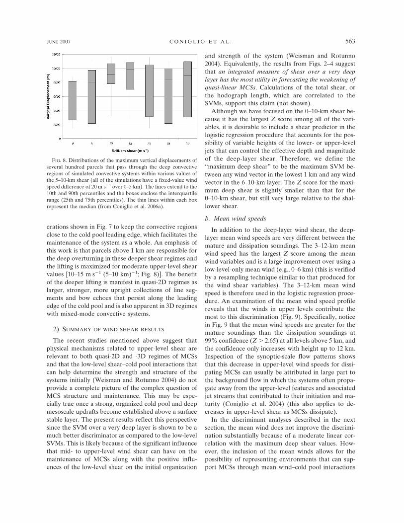
erations shown in Fig. 7 to keep the convective regionsclose to the cold pool leading edge, which facilitates themaintenance of the system as a whole. An emphasis ofthis work is that parcels above 1 km are responsible forthe deep overturning in these deeper shear regimes andthe lifting is maximized for moderate upper-level shearvalues [10–15 m s�1 (5–10 km)�1; Fig. 8)]. The benefitof the deeper lifting is manifest in quasi-2D regimes aslarger, stronger, more upright collections of line seg-ments and bow echoes that persist along the leadingedge of the cold pool and is also apparent in 3D regimeswith mixed-mode convective systems.

2) SUMMARY OF WIND SHEAR RESULTS

The recent studies mentioned above suggest thatphysical mechanisms related to upper-level shear arerelevant to both quasi-2D and -3D regimes of MCSsand that the low-level shear–cold pool interactions thatcan help determine the strength and structure of thesystems initially (Weisman and Rotunno 2004) do notprovide a complete picture of the complex question ofMCS structure and maintenance. This may be espe-cially true once a strong, organized cold pool and deepmesoscale updrafts become established above a surfacestable layer. The present results reflect this perspectivesince the SVM over a very deep layer is shown to be amuch better discriminator as compared to the low-levelSVMs. This is likely because of the significant influencethat mid- to upper-level wind shear can have on themaintenance of MCSs along with the positive influ-ences of the low-level shear on the initial organization

and strength of the system (Weisman and Rotunno2004). Equivalently, the results from Figs. 2–4 suggestthat an integrated measure of shear over a very deeplayer has the most utility in forecasting the weakening ofquasi-linear MCSs. Calculations of the total shear, orthe hodograph length, which are correlated to theSVMs, support this claim (not shown).

Although we have focused on the 0–10-km shear be-cause it has the largest Z score among all of the vari-ables, it is desirable to include a shear predictor in thelogistic regression procedure that accounts for the pos-sibility of variable heights of the lower- or upper-leveljets that can control the effective depth and magnitudeof the deep-layer shear. Therefore, we define the“maximum deep shear” to be the maximum SVM be-tween any wind vector in the lowest 1 km and any windvector in the 6–10-km layer. The Z score for the maxi-mum deep shear is slightly smaller than that for the0–10-km shear, but still very large relative to the shal-lower shear.

b. Mean wind speeds

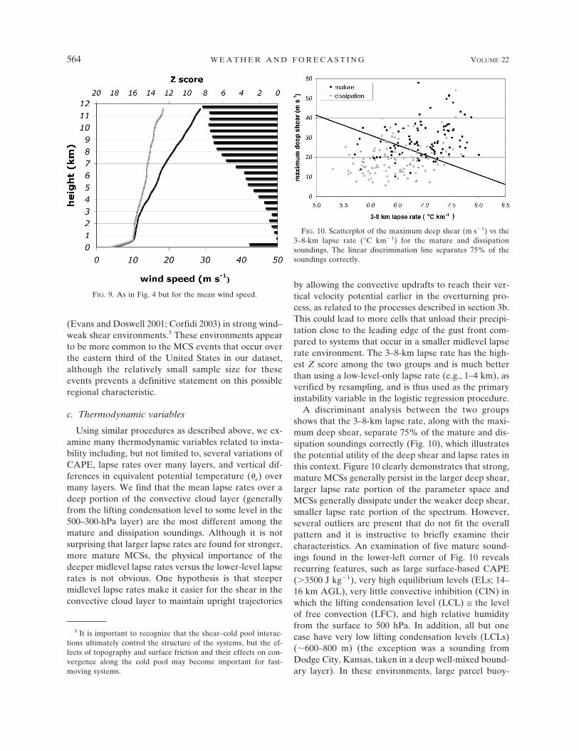
In addition to the deep-layer wind shear, the deep-layer mean wind speeds are very different between themature and dissipation soundings. The 3–12-km meanwind speed has the largest Z score among the meanwind variables and is a large improvement over using alow-level-only mean wind (e.g., 0–6 km) (this is verifiedby a resampling technique similar to that produced forthe wind shear variables). The 3–12-km mean windspeed is therefore used in the logistic regression proce-dure. An examination of the mean wind speed profilereveals that the winds in upper levels contribute themost to this discrimination (Fig. 9). Specifically, noticein Fig. 9 that the mean wind speeds are greater for themature soundings than the dissipation soundings at99% confidence (Z � 2.65) at all levels above 5 km, andthe confidence only increases with height up to 12 km.Inspection of the synoptic-scale flow patterns showsthat this decrease in upper-level wind speeds for dissi-pating MCSs can usually be attributed in large part tothe background flow in which the systems often propa-gate away from the upper-level features and associatedjet streams that contributed to their initiation and ma-turity (Coniglio et al. 2004) (this also applies to de-creases in upper-level shear as MCSs dissipate).

In the discriminant analyses described in the nextsection, the mean wind does not improve the discrimi-nation substantially because of a moderate linear cor-relation with the maximum deep shear values. How-ever, the inclusion of the mean winds allows for thepossibility of representing environments that can sup-port MCSs through mean wind–cold pool interactions

FIG. 8. Distributions of the maximum vertical displacements ofseveral hundred parcels that pass through the deep convectiveregions of simulated convective systems within various values ofthe 5–10-km shear (all of the simulations have a fixed-value windspeed difference of 20 m s�1 over 0–5 km). The lines extend to the10th and 90th percentiles and the boxes enclose the interquartilerange (25th and 75th percentiles). The thin lines within each boxrepresent the median (from Coniglio et al. 2006a).


(Evans and Doswell 2001; Corfidi 2003) in strong wind–weak shear environments.5 These environments appearto be more common to the MCS events that occur overthe eastern third of the United States in our dataset,although the relatively small sample size for theseevents prevents a definitive statement on this possibleregional characteristic.

c. Thermodynamic variables

Using similar procedures as described above, we ex-amine many thermodynamic variables related to insta-bility including, but not limited to, several variations ofCAPE, lapse rates over many layers, and vertical dif-ferences in equivalent potential temperature (�e) overmany layers. We find that the mean lapse rates over adeep portion of the convective cloud layer (generallyfrom the lifting condensation level to some level in the500–300-hPa layer) are the most different among themature and dissipation soundings. Although it is notsurprising that larger lapse rates are found for stronger,more mature MCSs, the physical importance of thedeeper midlevel lapse rates versus the lower-level lapserates is not obvious. One hypothesis is that steepermidlevel lapse rates make it easier for the shear in theconvective cloud layer to maintain upright trajectories

by allowing the convective updrafts to reach their ver-tical velocity potential earlier in the overturning pro-cess, as related to the processes described in section 3b.This could lead to more cells that unload their precipi-tation close to the leading edge of the gust front com-pared to systems that occur in a smaller midlevel lapserate environment. The 3–8-km lapse rate has the high-est Z score among the two groups and is much betterthan using a low-level-only lapse rate (e.g., 1–4 km), asverified by resampling, and is thus used as the primaryinstability variable in the logistic regression procedure.

A discriminant analysis between the two groupsshows that the 3–8-km lapse rate, along with the maxi-mum deep shear, separate 75% of the mature and dis-sipation soundings correctly (Fig. 10), which illustratesthe potential utility of the deep shear and lapse rates inthis context. Figure 10 clearly demonstrates that strong,mature MCSs generally persist in the larger deep shear,larger lapse rate portion of the parameter space andMCSs generally dissipate under the weaker deep shear,smaller lapse rate portion of the spectrum. However,several outliers are present that do not fit the overallpattern and it is instructive to briefly examine theircharacteristics. An examination of five mature sound-ings found in the lower-left corner of Fig. 10 revealsrecurring features, such as large surface-based CAPE(�3500 J kg�1), very high equilibrium levels (ELs; 14–16 km AGL), very little convective inhibition (CIN) inwhich the lifting condensation level (LCL) ≅ the levelof free convection (LFC), and high relative humidityfrom the surface to 500 hPa. In addition, all but onecase have very low lifting condensation levels (LCLs)(�600–800 m) (the exception was a sounding fromDodge City, Kansas, taken in a deep well-mixed bound-ary layer). In these environments, large parcel buoy-

5 It is important to recognize that the shear–cold pool interac-tions ultimately control the structure of the systems, but the ef-fects of topography and surface friction and their effects on con-vergence along the cold pool may become important for fast-moving systems.

FIG. 9. As in Fig. 4 but for the mean wind speed.

FIG. 10. Scatterplot of the maximum deep shear (m s�1) vs the3–8-km lapse rate (°C km�1) for the mature and dissipationsoundings. The linear discrimination line separates 75% of thesoundings correctly.


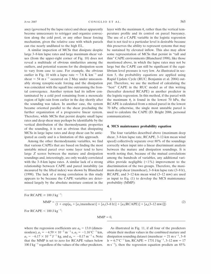
ancy (governed by the lapse rates) and shear apparentlybecome unnecessary to retrigger and organize convec-tion along the cold pool, or any other linear forcingmechanism, given the relative ease with which parcelscan rise nearly undiluted to the high EL.

A similar inspection of MCSs that dissipate despitelarge 3–8-km lapse rates and large maximum shear val-ues (from the upper-right corner of Fig. 10) does notreveal a multitude of obvious similarities among theoutliers, and potential reasons for the dissipation seemto vary from case to case. For example, the obviousoutlier in Fig. 10 with a lapse rate 7.6 K km�1 andshear 54 m s�1 occurred on 2 May under unseason-ably strong synoptic-scale forcing and the dissipationwas coincident with the squall line outrunning the fron-tal convergence. Another system had its inflow con-taminated by a cold pool remaining from a mesoscaleregion of light rain from earlier in the day shortly afterthe sounding was taken. In another case, the systembecame oriented parallel to the shear precluding thefurther organization of a progressive linear system.Therefore, while MCSs that persist despite small lapserates and deep shear may perhaps be identifiable by thevertical distribution of the thermodynamic propertiesof the sounding, it is not as obvious that dissipatingMCSs in large lapse rates and deep shear can be antic-ipated as easily and is a limitation of this approach.

Among the other thermodynamic variables, we findthat various CAPEs that are based on finding the mostunstable mixed parcel over some layer tend to havelarge Z scores between the mature and dissipationsoundings and, interestingly, are only weakly correlatedwith the 3–8-km lapse rates. A similar lack of a strongrelationship between CAPE and parcel instability (asmeasured by the lifted index) was shown by Blanchard(1998). The lack of a strong correlation in this studyappears to be because the CAPE variables are deter-mined largely by the absolute moisture content in the

layer with the maximum �e rather than the vertical tem-perature profile and its control on parcel buoyancy.The use of a CAPE variable in the logistic regressionthat is not tied to a particular level is desirable becausethis preserves the ability to represent systems that maybe sustained by elevated inflow. This also may allowsome representation of MCSs that persist in “tall andthin” CAPE environments (Blanchard 1998), like thosementioned above, in which the lapse rates may not belarge but the CAPE can still be significant if the equi-librium level pressure is very low. As illustrated in sec-tion 5, the probability equations are applied usingRapid Update Cycle (RUC; Benjamin et al. 2004) out-put. Therefore, we use the method of calculating the“best” CAPE in the RUC model as of this writing(hereafter denoted RCAPE) as another predictor inthe logistic regression. In this method, if the parcel withthe maximum �e is found in the lowest 70 hPa, theRCAPE is calculated from a mixed parcel in the lowest70 hPa; otherwise, the single most unstable parcel isused to calculate the CAPE (D. Bright 2006, personalcommunication).

4. MCS maintenance probability equation

The four variables described above (maximum deepshear, 3–8-km lapse rate, RCAPE, 3–12-km mean windspeed) collectively separate over 80% of the soundingscorrectly when input into a linear discriminant analysisbetween the mature and dissipation soundings. It isworth noting that, because of the mutual correlationsamong the hundreds of variables, any additional vari-ables provide negligible (�1%) improvement to thediscrimination of the two groups. Therefore, the maxi-mum deep shear (maxshear), 3–8-km lapse rate (3–8 lr),RCAPE, and 3–12-km mean wind (3–12 mw) are usedas input to Eq. (1) to develop the MCS maintenanceprobability (MMP):

For RCAPE � 100 J kg�1:

MMP �1

�1 � exp�a0 � �a1�maxshear�� a2�3–8 lr�� a3�RCAPE�� a4�3–12 mw��2�

For RCAPE � 100 J kg�1:

MMP � 0,

where the regression coefficients are a0 � 13.0 (dimen-sionless), a1 � �4.59 � 10�2 m�1 s, a2 � �1.16°C�1 km,a3 � �6.17 � 10�4 J�1 kg, and a4 � �0.17 m�1 s. Notethat the MMP is set to zero for RCAPE values below100 J kg�1 regardless of the values of the other predictors.

As illustrated in Fig. 11, if all four of the predictorsobtain their median values in the combined mature anddissipation sounding dataset (maxshear � 21 m s�1, 3–8lr � 6.7°C�1 km, RCAPE � 1731 J kg�1, 3–12 mw � 17m s�1), then the regression equation predicts an 85%


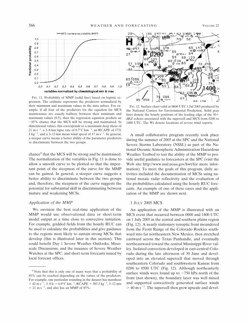
chance6 that the MCS will be strong and be maintained.The normalization of the variables in Fig. 11 is done toallow a smooth curve to be plotted so that the impor-tant point of the steepness of the curve for the MMPcan be gained. In general, a steeper curve suggests abetter ability to discriminate between the two groupsand, therefore, the steepness of the curve suggests thepotential for substantial skill in discriminating betweenmature and weakening MCSs.

Application of the MMP

We envision the best real-time application of theMMP would use observational data or short-termmodel output at a time close to convective initiation.For example, gridded fields from the hourly RUC canbe used to calculate the probabilities and give guidanceto the regions most likely to sustain strong MCSs thatdevelop (this is illustrated later in this section). Thiscould benefit Day 1 Severe Weather Outlooks, Meso-scale Discussions, and the issuance of Severe WeatherWatches at the SPC, and short-term forecasts issued bylocal forecast offices.

A small collaborative program recently took placeduring the summer of 2005 at the SPC and the NationalSevere Storms Laboratory (NSSL) as part of the Na-tional Oceanic Atmospheric Administration HazardousWeather Testbed to test the ability of the MMP to pro-vide useful guidance to forecasters at the SPC (visit theWeb site http://www.nssl.noaa.gov/hwt/for more infor-mation). To meet the goals of this program, daily ac-tivities included the documentation of MCSs using na-tional mosaic radar reflectivity and the evaluation ofthe probabilities calculated using the hourly RUC fore-casts. An example of one of these cases and the appli-cation of the MMP are shown next.

1 JULY 2005 MCS

An application of the MMP is illustrated with anMCS event that occurred between 0000 and 1400 UTCon 1 July 2005 in the central and southern plains region(Fig. 12). A nearly stationary synoptic front meanderedfrom the Front Range of the Colorado Rockies south-ward into far northeastern New Mexico, then stretchedeastward across the Texas Panhandle, and eventuallynortheastward toward the central Mississippi River val-ley. Isolated convection developed in east-central Colo-rado during the late afternoon of 30 June and devel-oped into an elevated supercell that moved throughsoutheastern Colorado and southwestern Kansas from0200 to 0500 UTC (Fig. 12). Although northeasterlysurface winds were found up to �750 hPa north of thefront (not shown), the boundary layer was well mixedand supported convectively generated surface winds� 40 m s�1. The supercell then grew upscale and devel-

6 Note that this is only one of many ways that a probability of85% can be reached depending on the values of the predictors.For example, one particular sounding in the dataset has maxshear� 42 m s�1, 3–8 lr � 6.9°C km�1, RCAPE � 383 J kg�1, 3–12 mw� 21 m s�1, and also has an MMP of 85%.

FIG. 11. Probability of MMP (solid line) based on logistic re-gression. The ordinate represents the predictors normalized bytheir minimum and maximum values in the data subset. For ex-ample, if all four of the predictors for the equation for MCSmaintenance are exactly halfway between their minimum andmaximum values (0.5), then the regression equation predicts an�85% chance that the MCS will be strong and maintained. Indimensional values, this corresponds to a maximum deep shear of21 m s�1, a 3–8-km lapse rate of 6.7°C km�1, an RCAPE of 1731J kg�1, and a 3–12-km mean wind speed of 17 m s�1. In general,a steeper curve means a better ability of the parameter predictorsto discriminate between the two groups.

FIG. 12. Surface chart valid at 0600 UTC 1 Jul 2005 produced bythe National Centers for Environmental Prediction. Solid graylines denote the hourly positions of the leading edge of the 50�dBZ echoes associated with the supercell and MCS from 0200 to1400 UTC. The Ws denote locations of severe wind reports.


oped linear characteristics as it entered Oklahoma after0600 UTC, with a continuation of the severe surfacewinds north of the front (Fig. 12).

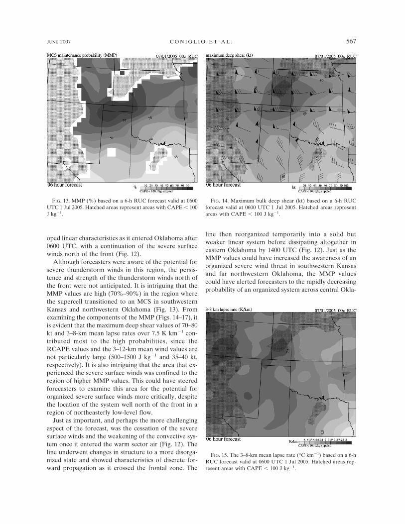
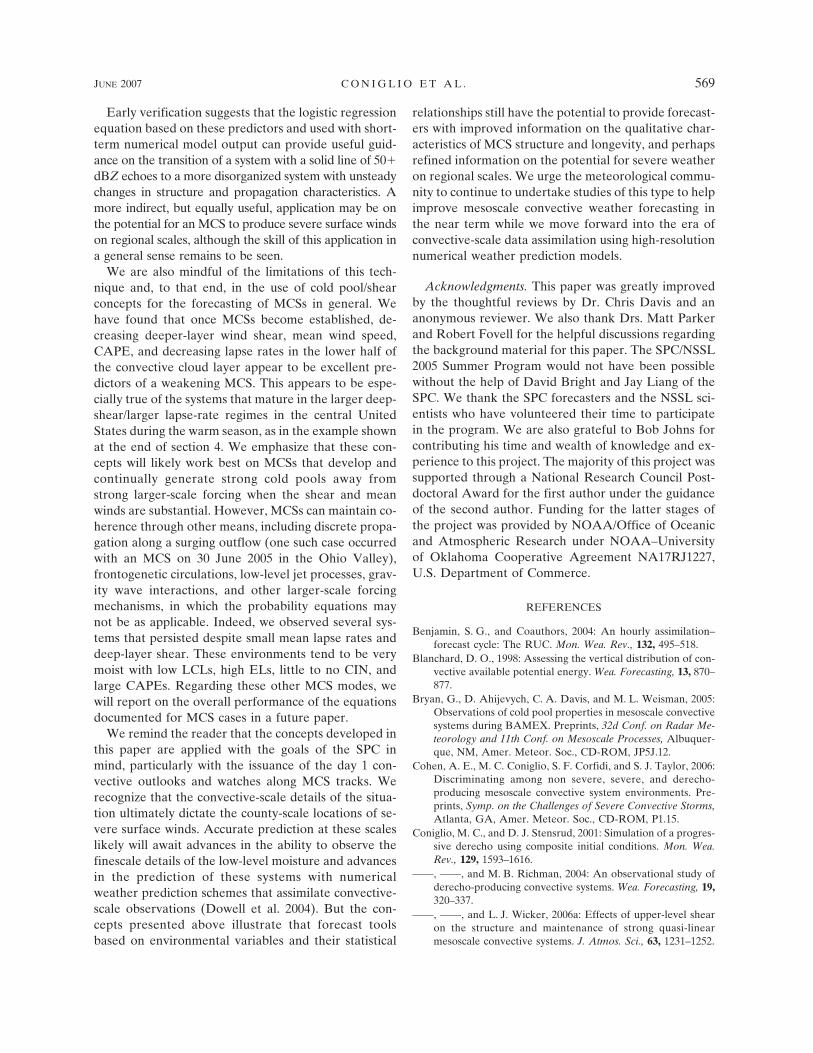
Although forecasters were aware of the potential forsevere thunderstorm winds in this region, the persis-tence and strength of the thunderstorm winds north ofthe front were not anticipated. It is intriguing that theMMP values are high (70%–90%) in the region wherethe supercell transitioned to an MCS in southwesternKansas and northwestern Oklahoma (Fig. 13). Fromexamining the components of the MMP (Figs. 14–17), itis evident that the maximum deep shear values of 70–80kt and 3–8-km mean lapse rates over 7.5 K km�1 con-tributed most to the high probabilities, since theRCAPE values and the 3–12-km mean wind values arenot particularly large (500–1500 J kg�1 and 35–40 kt,respectively). It is also intriguing that the area that ex-perienced the severe surface winds was confined to theregion of higher MMP values. This could have steeredforecasters to examine this area for the potential fororganized severe surface winds more critically, despitethe location of the system well north of the front in aregion of northeasterly low-level flow.

Just as important, and perhaps the more challengingaspect of the forecast, was the cessation of the severesurface winds and the weakening of the convective sys-tem once it entered the warm sector air (Fig. 12). Theline underwent changes in structure to a more disorga-nized state and showed characteristics of discrete for-ward propagation as it crossed the frontal zone. The

line then reorganized temporarily into a solid butweaker linear system before dissipating altogether ineastern Oklahoma by 1400 UTC (Fig. 12). Just as theMMP values could have increased the awareness of anorganized severe wind threat in southwestern Kansasand far northwestern Oklahoma, the MMP valuescould have alerted forecasters to the rapidly decreasingprobability of an organized system across central Okla-

FIG. 13. MMP (%) based on a 6-h RUC forecast valid at 0600UTC 1 Jul 2005. Hatched areas represent areas with CAPE � 100J kg�1.

FIG. 14. Maximum bulk deep shear (kt) based on a 6-h RUCforecast valid at 0600 UTC 1 Jul 2005. Hatched areas representareas with CAPE � 100 J kg�1.

FIG. 15. The 3–8-km mean lapse rate (°C km�1) based on a 6-hRUC forecast valid at 0600 UTC 1 Jul 2005. Hatched areas rep-resent areas with CAPE � 100 J kg�1.


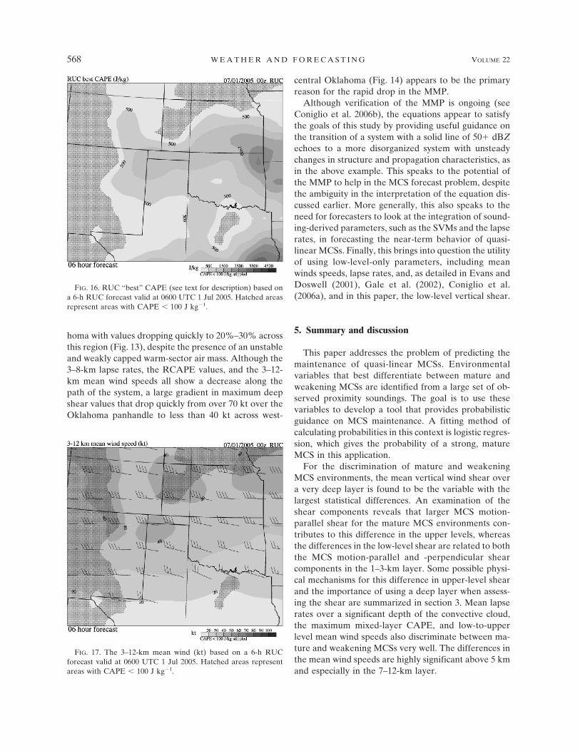
homa with values dropping quickly to 20%–30% acrossthis region (Fig. 13), despite the presence of an unstableand weakly capped warm-sector air mass. Although the3–8-km lapse rates, the RCAPE values, and the 3–12-km mean wind speeds all show a decrease along thepath of the system, a large gradient in maximum deepshear values that drop quickly from over 70 kt over theOklahoma panhandle to less than 40 kt across west-

central Oklahoma (Fig. 14) appears to be the primaryreason for the rapid drop in the MMP.

Although verification of the MMP is ongoing (seeConiglio et al. 2006b), the equations appear to satisfythe goals of this study by providing useful guidance onthe transition of a system with a solid line of 50� dBZechoes to a more disorganized system with unsteadychanges in structure and propagation characteristics, asin the above example. This speaks to the potential ofthe MMP to help in the MCS forecast problem, despitethe ambiguity in the interpretation of the equation dis-cussed earlier. More generally, this also speaks to theneed for forecasters to look at the integration of sound-ing-derived parameters, such as the SVMs and the lapserates, in forecasting the near-term behavior of quasi-linear MCSs. Finally, this brings into question the utilityof using low-level-only parameters, including meanwinds speeds, lapse rates, and, as detailed in Evans andDoswell (2001), Gale et al. (2002), Coniglio et al.(2006a), and in this paper, the low-level vertical shear.

5. Summary and discussion

This paper addresses the problem of predicting themaintenance of quasi-linear MCSs. Environmentalvariables that best differentiate between mature andweakening MCSs are identified from a large set of ob-served proximity soundings. The goal is to use thesevariables to develop a tool that provides probabilisticguidance on MCS maintenance. A fitting method ofcalculating probabilities in this context is logistic regres-sion, which gives the probability of a strong, matureMCS in this application.

For the discrimination of mature and weakeningMCS environments, the mean vertical wind shear overa very deep layer is found to be the variable with thelargest statistical differences. An examination of theshear components reveals that larger MCS motion-parallel shear for the mature MCS environments con-tributes to this difference in the upper levels, whereasthe differences in the low-level shear are related to boththe MCS motion-parallel and -perpendicular shearcomponents in the 1–3-km layer. Some possible physi-cal mechanisms for this difference in upper-level shearand the importance of using a deep layer when assess-ing the shear are summarized in section 3. Mean lapserates over a significant depth of the convective cloud,the maximum mixed-layer CAPE, and low-to-upperlevel mean wind speeds also discriminate between ma-ture and weakening MCSs very well. The differences inthe mean wind speeds are highly significant above 5 kmand especially in the 7–12-km layer.

FIG. 16. RUC “best” CAPE (see text for description) based ona 6-h RUC forecast valid at 0600 UTC 1 Jul 2005. Hatched areasrepresent areas with CAPE � 100 J kg�1.

FIG. 17. The 3–12-km mean wind (kt) based on a 6-h RUCforecast valid at 0600 UTC 1 Jul 2005. Hatched areas representareas with CAPE � 100 J kg�1.


Early verification suggests that the logistic regressionequation based on these predictors and used with short-term numerical model output can provide useful guid-ance on the transition of a system with a solid line of 50�dBZ echoes to a more disorganized system with unsteadychanges in structure and propagation characteristics. Amore indirect, but equally useful, application may be onthe potential for an MCS to produce severe surface windson regional scales, although the skill of this application ina general sense remains to be seen.

We are also mindful of the limitations of this tech-nique and, to that end, in the use of cold pool/shearconcepts for the forecasting of MCSs in general. Wehave found that once MCSs become established, de-creasing deeper-layer wind shear, mean wind speed,CAPE, and decreasing lapse rates in the lower half ofthe convective cloud layer appear to be excellent pre-dictors of a weakening MCS. This appears to be espe-cially true of the systems that mature in the larger deep-shear/larger lapse-rate regimes in the central UnitedStates during the warm season, as in the example shownat the end of section 4. We emphasize that these con-cepts will likely work best on MCSs that develop andcontinually generate strong cold pools away fromstrong larger-scale forcing when the shear and meanwinds are substantial. However, MCSs can maintain co-herence through other means, including discrete propa-gation along a surging outflow (one such case occurredwith an MCS on 30 June 2005 in the Ohio Valley),frontogenetic circulations, low-level jet processes, grav-ity wave interactions, and other larger-scale forcingmechanisms, in which the probability equations maynot be as applicable. Indeed, we observed several sys-tems that persisted despite small mean lapse rates anddeep-layer shear. These environments tend to be verymoist with low LCLs, high ELs, little to no CIN, andlarge CAPEs. Regarding these other MCS modes, wewill report on the overall performance of the equationsdocumented for MCS cases in a future paper.

We remind the reader that the concepts developed inthis paper are applied with the goals of the SPC inmind, particularly with the issuance of the day 1 con-vective outlooks and watches along MCS tracks. Werecognize that the convective-scale details of the situa-tion ultimately dictate the county-scale locations of se-vere surface winds. Accurate prediction at these scaleslikely will await advances in the ability to observe thefinescale details of the low-level moisture and advancesin the prediction of these systems with numericalweather prediction schemes that assimilate convective-scale observations (Dowell et al. 2004). But the con-cepts presented above illustrate that forecast toolsbased on environmental variables and their statistical

relationships still have the potential to provide forecast-ers with improved information on the qualitative char-acteristics of MCS structure and longevity, and perhapsrefined information on the potential for severe weatheron regional scales. We urge the meteorological commu-nity to continue to undertake studies of this type to helpimprove mesoscale convective weather forecasting inthe near term while we move forward into the era ofconvective-scale data assimilation using high-resolutionnumerical weather prediction models.

Acknowledgments. This paper was greatly improvedby the thoughtful reviews by Dr. Chris Davis and ananonymous reviewer. We also thank Drs. Matt Parkerand Robert Fovell for the helpful discussions regardingthe background material for this paper. The SPC/NSSL2005 Summer Program would not have been possiblewithout the help of David Bright and Jay Liang of theSPC. We thank the SPC forecasters and the NSSL sci-entists who have volunteered their time to participatein the program. We are also grateful to Bob Johns forcontributing his time and wealth of knowledge and ex-perience to this project. The majority of this project wassupported through a National Research Council Post-doctoral Award for the first author under the guidanceof the second author. Funding for the latter stages ofthe project was provided by NOAA/Office of Oceanicand Atmospheric Research under NOAA–Universityof Oklahoma Cooperative Agreement NA17RJ1227,U.S. Department of Commerce.

REFERENCES

Benjamin, S. G., and Coauthors, 2004: An hourly assimilation–forecast cycle: The RUC. Mon. Wea. Rev., 132, 495–518.

Blanchard, D. O., 1998: Assessing the vertical distribution of con-vective available potential energy. Wea. Forecasting, 13, 870–877.

Bryan, G., D. Ahijevych, C. A. Davis, and M. L. Weisman, 2005:Observations of cold pool properties in mesoscale convectivesystems during BAMEX. Preprints, 32d Conf. on Radar Me-teorology and 11th Conf. on Mesoscale Processes, Albuquer-que, NM, Amer. Meteor. Soc., CD-ROM, JP5J.12.

Cohen, A. E., M. C. Coniglio, S. F. Corfidi, and S. J. Taylor, 2006:Discriminating among non severe, severe, and derecho-producing mesoscale convective system environments. Pre-prints, Symp. on the Challenges of Severe Convective Storms,Atlanta, GA, Amer. Meteor. Soc., CD-ROM, P1.15.

Coniglio, M. C., and D. J. Stensrud, 2001: Simulation of a progres-sive derecho using composite initial conditions. Mon. Wea.Rev., 129, 1593–1616.

——, ——, and M. B. Richman, 2004: An observational study ofderecho-producing convective systems. Wea. Forecasting, 19,320–337.

——, ——, and L. J. Wicker, 2006a: Effects of upper-level shearon the structure and maintenance of strong quasi-linearmesoscale convective systems. J. Atmos. Sci., 63, 1231–1252.


——, M. Bardon, K. Virts, and S. J. Weiss, 2006b: Forecasting themaintenance of mesoscale convective systems. Preprints, 23dConf. on Severe Local Storms, St. Louis, MO, Amer. Meteor.Soc., CD-ROM, P2.3.

Corfidi, S. F., 2003: Cold pools and MCS propagation: Forecastingthe motion of downwind-developing MCSs. Wea. Forecast-ing, 18, 997–1017.

Cotton, W. R., M.-S. Lin, R. L. McAnelly, and C. J. Tremback,1989: A composite model of mesoscale convective complexes.Mon. Wea. Rev., 117, 765–783.

Davis, C. A., and Coauthors, 2004: The Bow-Echo and MCV Ex-periment (BAMEX): Observations and opportunities. Bull.Amer. Meteor. Soc., 85, 1075–1093.

Done, J., C. A. Davis, and M. L. Weisman, 2004: The next gen-eration of NWP: Explicit forecasts of convection using theWeather Research and Forecasting (WRF) model. Atmos.Sci. Lett., 5, 110–117.

Dowell, D. C., F. Zhang, L. J. Wicker, C. Snyder, and N. A.Crook, 2004: Wind and temperature retrievals in the 17 May1981 Arcadia, Oklahoma, supercell: Ensemble Kalman filterexperiments. Mon. Wea. Rev., 132, 1982–2005.

Evans, J. S., and C. A. Doswell, 2001: Examination of derechoenvironments using proximity soundings. Wea. Forecasting,16, 329–342.

Fovell, R. G., and P. S. Daily, 1995: The temporal behavior ofnumerically simulated multicell-type storms. Part I: Modes ofbehavior. J. Atmos. Sci., 52, 2073–2095.

——, B. Rubin-Oster, and S. Kim, 2005: A discretely propagatingnocturnal Oklahoma squall line: Observations and numericalsimulations. Preprints, 22d Conf. on Severe Local Storms,Hyannis, MA, Amer. Meteor. Soc., CD-ROM, 6.1.

Fritsch, J. M., and G. S. Forbes, 2001: Mesoscale convective sys-tems. Severe Convective Storms, Meteor. Monogr., No. 50,Amer. Meteor. Soc., 323–357.

Gale, J. J., W. A. Gallus Jr., and K. A. Jungbluth, 2002: Towardimproved prediction of mesoscale convective system dissipa-tion. Wea. Forecasting, 17, 856–872.

Kain, J. S., S. J. Weiss, M. E. Baldwin, G. W. Carbin, D. Bright,J. J. Levit, and J. A. Hart, 2005: Evaluating high-resolutionconfigurations of the WRF model that are used to forecast

severe convective weather: The 2005 SPC/NSSL Spring Ex-periment. Preprints, 21st Conf. on Weather Analysis andForecasting and 17th Conf. on Numerical Weather Prediction,Washington, DC, Amer. Meteor. Soc., CD-ROM, 2A.5.

Moncrieff, M. W., and C. Liu, 1999: Convection initiation by den-sity currents: Role of convergence, shear, and dynamical or-ganization. Mon. Wea. Rev., 127, 2455–2464.

Parker, M. D., and R. H. Johnson, 2000: Organizational modes ofmidlatitude mesoscale convective systems. Mon. Wea. Rev.,128, 3413–3436.

——, and ——, 2004a: Structures and dynamics of quasi-2D meso-scale convective systems. J. Atmos. Sci., 61, 545–567.

——, and ——, 2004b: Simulated convective lines with leadingprecipitation. Part I: Governing dynamics. J. Atmos. Sci., 61,1637–1655.

——, and ——, 2004c: Simulated convective lines with leadingprecipitation. Part II: Evolution and maintenance. J. Atmos.Sci., 61, 1656–1673.

Shapiro, A., 1992: A hydrodynamical model of shear flow oversemi-infinite barriers with application to density currents. J.Atmos. Sci., 49, 2293–2305.

Stensrud, D. J., M. C. Coniglio, R. Davies-Jones, and J. Evans,2005: Comments on ‘“A theory for strong long-lived squalllines’ revisted.” J. Atmos. Sci., 62, 2989–2996.

Trier, S. B., and C. A. Davis, 2005: Propagating nocturnal convec-tion within a 7-day WRF–model simulation. Preprints, 32dConf. on Radar Meteorology and 11th Conf. on MesoscaleProcesses, Albuquerque, NM, Amer. Meteor. Soc., CD-ROM, P2M.1.

Weisman, M. L., and R. Rotunno, 2004: “A theory for stronglong-lived squall lines” revisited. J. Atmos. Sci., 61, 361–382.

——, J. B. Klemp, and R. Rotunno, 1988: Structure and evolutionof numerically simulated squall lines. J. Atmos. Sci., 45, 1990–2013.

Wilks, D. S., 1995: Statistical Methods in the Atmospheric Sciences.Academic Press, 467 pp.

Zipser, K. A., 1982: Use of a conceptual model of the life cycle ofmesoscale convective systems to improve very-short-rangeforecasts. Nowcasting, K. Browning, Ed., Academic Press,191–204.


Documents

Forecasting the Maintenance of Quasi-Linear Mesoscale Convective Systems