Department of Economics and Business Economics

Aarhus University

Fuglesangs Allé 4

DK-8210 Aarhus V

Denmark

Email: oekonomi@au.dk

Tel: +45 8716 5515

Forecasting the Global Mean Sea Level, a Continuous-Time

State-Space Approach

Lorenzo Boldrini

CREATES Research Paper 2015-40

Forecasting the Global Mean Sea Level,

a Continuous-Time State-Space Approach

Lorenzo Boldrini ∗

August 27, 2015

Abstract

In this paper we propose a continuous-time, Gaussian, linear, state-space system tomodel the relation between global mean sea level (GMSL) and the global mean tem-perature (GMT), with the aim of making long-term projections for the GMSL. Weprovide a justification for the model specification based on popular semi-empiricalmethods present in the literature and on zero-dimensional energy balance models.We show that some of the models developed in the literature on semi-empirical mod-els can be analysed within this framework. We use the sea-level data reconstructiondeveloped in Church and White (2011) and the temperature reconstruction fromHansen et al. (2010). We compare the forecasting performance of the proposedspecification to the procedures developed in Rahmstorf (2007b) and Vermeer andRahmstorf (2009). Finally, we compute projections for the sea-level rise conditionalon the 21st century SRES temperature scenarios of the IPCC fourth assessmentreport. Furthermore, we propose a bootstrap procedure to compute confidence in-tervals for the projections, based on the method introduced in Rodriguez and Ruiz(2009).

Keywords: energy balance model, semi-empirical model, state-space system, Kalmanfilter, forecasting, temperature, sea level, bootstrap.JEL classification: C32.

∗Aarhus University, Department of Economics and Business Economics, CREATES - Center for Re-search in Econometric Analysis of Time Series, Fuglesangs Alle 4, 8210 Aarhus V, Denmark. Email:lboldrini@econ.au.dk. The author acknowledges support from CREATES - Center for Research in Econo-metric Analysis of Time Series (DNRF78), funded by the Danish National Research Foundation.

1 Introduction

Climate changes, the increase in the global temperature and sea level are long-standingtopics. Monitoring and predicting the rise in the sea level is of great importance dueto its close relation with global climate changes and the socio-economic effects it entails.In particular, the sea-level rise has direct consequences for populations living near thecurrent mean sea level, Anthoff et al. (2006), Anthoff et al. (2010), Arnell et al. (2005),Sugiyama et al. (2008). Physical and statistical models are needed to measure the rate ofchange of the sea level and understand its relation to anthropogenic and natural causes.

In this paper we propose a statistical framework to model the relation between theglobal mean sea level (GMSL) and the global mean temperature (GMT), with the aimof making long-term projections for the GMSL. The model belongs to the class of semi-empirical models. We provide a justification for the model specification based on popularsemi-empirical methods present in the literature and on zero-dimensional energy balancemodels. We show that some of the semi-empirical models developed in the literature tostudy the relation between sea-level rise and temperature can be analysed within thisframework.

To date, there are two methods of estimating the sea-level rise as a function of climateforcing. The conventional approach, used by the Intergovernmental Panel on ClimateChange (IPCC) climate assessments, is to use process-based models to estimate contri-butions from the sea-level components and then sum them to obtain an estimate of thesea-level increase, see for instance Meehl et al. (2007), Meehl et al. (2007), Pardaens et al.(2011), Solomon et al. (2009). Variations in the sea level originate from steric, eustatic,and non-climate changes. By steric, we mean sea-level variations due to ocean volumechanges, resulting from temperature (thermosteric) and salinity (halosteric) variations.By eustatic, we mean variations in the mass of the oceans as a result of water exchangesbetween the oceans and other surface reservoirs (ice sheets, glaciers, land water reservoirs,and the atmosphere)1. By non-climate causes we mean variations in the quantity of wa-ter in the oceans due to human impact, such as the building of dams and the extractionof groundwater. However, the theoretical understanding of the different contributors isincomplete, as IPCC models under-predict rates of sea-level increase.

The alternative way of making projections of the sea level is the class of semi-empiricalmodels. These models analyse statistical relationships using physically plausible modelsof reduced complexity in which the sea-level rate of change depends on the global tem-perature. The main idea behind semi-empirical models is that the steric and eustaticcontributors to the sea level (the major ones) respond to changes in the global tempera-ture. The first semi-empirical model was proposed by Gornitz et al. (1982) who specify alinear relation between sea level and temperature. Some more recent models where devel-oped by specifying a differential equation, relating the sea level to temperature or otherclimate forcing. Representative examples are Rahmstorf (2007b), Vermeer and Rahmstorf(2009), Grinsted et al. (2010), Kemp et al. (2011), Jevrejeva et al. (2009), Jevrejeva et al.(2010), Jevrejeva et al. (2012b), Jevrejeva et al. (2012a).

All semi-empirical models project higher sea-level rise, for the 21st century, that thelast generation of process-based models, summarized in the IPCC Fourth Assessment Re-port, see for instance Moore et al. (2013), Cazenave and Nerem (2004), Munk (2002), and

1In this paper we adopt the same definitions of steric and eustatic used in Cazenave and Nerem (2004).

1

Rahmstorf (2007b). A comprehensive survey on the different process-based and semi-empirical models can be found in Moore et al. (2013).

We propose a state-space approach to forecast the global mean sea level, conditionalon the global mean temperature. State-space systems allow to address the problems ofsmoothing, detrending, and parameter estimation in a unique framework. We considerin particular continuous-time, linear, Gaussian state-space systems of the type describedin Bergstrom (1997). More specifically, the state vector follows a multivariate, Gaussian,OrnsteinUhlenbeck process. The discretised system preserves its linearity and Kalmanfiltering techniques apply. In particular, the Kalman filter is used for two tasks: the firstone is to compute the likelihood function of the state-space system, needed for parameterestimation, and the second one is to make forecasts of the sea level, conditional on thetemperature.

The statistical framework of state-space systems allows to distinguish between mea-surement noise and model uncertainty, through the measurement and state equations,respectively. Furthermore, in this setup it is possible to consider different levels of mea-surement noise for different points in time. In fact, the reconstructions of the sea level,in particular, are typically very noisy and the measurements uncertainty reflects, for in-stance, the changes in the measurement instruments throughout the decades, as well asthe changes in the data sources. In this study we use the sea-level reconstruction fromChurch and White (2011), who also provide an estimate of the uncertainty of their sea-level estimates. In the state-space approach these uncertainties (measured as standarddeviations) are directly used to parameterise the time-varying variances of the measure-ment errors of the sea-level time series. Temperature data are taken from Hansen et al.(2010). Both sea level and temperature data correspond to monthly reconstructions.

We provide a justification for the model specification based on popular semi-empiricalmethods present in the literature and on zero-dimensional energy balance models. In moredetail, we specified the system dynamics of sea level and temperature as well as the func-tional form linking these variables, consistently with the ones suggested by the existingliterature. We show that some of the semi-empirical models developed in the literatureto study the relation between sea level and temperature, can be analysed within thisframework.

Semi-empirical models are usually specified as differential equations, as in Rahmstorf(2007b), Vermeer and Rahmstorf (2009), Grinsted et al. (2010), Kemp et al. (2011), Jevre-jeva et al. (2009), Jevrejeva et al. (2010), Jevrejeva et al. (2012b), and Jevrejeva et al.(2012a). By specifying the state-space system in continuous time and then deriving theexact discrete-time system, we can make inference on the structural parameters drivingthe continuous-time process. A similar approach was used in Pretis (2015) (forthcoming),in which the author shows the equivalence of a two-component energy balance model toa cointegrated system. He then shows the exact mapping between the continuous-timesystem to the discrete-time one, that amounts to a cointegrated vector autoregressivesystem.

In the literature on semi-empirical models, state-space system representations andthe Kalman filter are often used with the aim of assimilating noisy measurements fromdifferent sources2. Such studies are for instance, Miller and Cane (1989) and Chan et al.

2In this context, assimilation usually refers to the filtering of a variable, measured at a specific pointin time and geographic location, by taking into account information from measurements taken at neigh-

2

(1996) who use the Kalman filter with an underlying physical model to assimilate averagesea-level anomalies from tide gauge measurements and Cane et al. (1996) and Hay et al.(2013).

The paper is organised as follows: in Section 2, we explain the statistical frameworkand introduce the model specification, showing how it relates to some important modelsin the literature; in Section 3, we describe the dataset; in Section 4, we illustrate the fore-casting procedures; in Section 5, we provide some details on the computational aspects ofthe analysis; in Section 6, we present results; finally, Section 7 concludes.

2 Model specification

2.1 Energy balance models and temperature dynamics

In this section we present the foundations for the temperature process used in the state-space model proposed in Section 2.3. This section draws heavily on North et al. (1981)and Imkeller (2001) and we refer the reader to these papers for more details. The start-ing model, for the temperature, belongs to the class of zero-dimensional energy balancemodels (EBMs), detailed in North et al. (1981), and whose review is based on the modelsintroduced in Budyko (1968), Budyko (1969), Budyko (1972), and Sellers (1969). Thesemodels are based on thermodynamic concepts and global radiative heat balance, for theEarth system. This type of models describe the global temperature process as (possiblystochastic) univariate, differential equations. In particular, the change in the Planet’sglobal temperature at time t is seen as a function of the difference between the incomingand outgoing radiation.

The incoming (absorbed) radiation Rin is caused by solar irradiance (i.e. the sun-light reaching the Earth) and is affected by the reflectivity of the Planet. The incomingradiation is then a function of the solar constant3 σ0, the albedo coefficient4 α, and theradius R of the Earth, in particular: Rin = σ0(1−α)πR2. The outgoing radiation Rout isassumed, for simplicity, to be black-body5 radiation, obeying the Stefan-Boltzmann law6.It is then a function of the absolute temperature T of the Planet and its radius R, inparticular: Rout = 4πR2kSBT

4.The analysis of zero-dimensional EBMs begins with the concept of global radiative

heat balance. In radiative equilibrium the rate at which solar radiation is absorbed bythe Planet matches the rate at which infrared radiation is emitted by it. The condition

bouring locations at the same point in time. If the filtered variables are output from the Kalman filter,the contribution of variable j to the estimate of variable i is given by element (i, j) of the Kalman gainmatrix.

3The solar constant is a measure of the mean solar electromagnetic radiation per unit area that wouldbe incident on a plane perpendicular to the sun rays.

4The term albedo, Latin for white, describes the average reflection coefficient of an object. Thegreenhouse effect, for instance, can lower the albedo of the Earth, and cause global warming.

5A black body is an idealized physical object that absorbs all incident electromagnetic radiation. Thetotal energy per unit of time, per unit of surface area, radiated by a black body depends solely on itsabsolute temperature and obeys the Stefan-Boltzman law.

6The Stefan-Boltzmann law describes the power radiated from a black body in terms of its thermo-dynamic temperature. The thermodynamic temperature (absolute temperature) is commonly expressedin Kelvin [K], where 0[K] = −273.15[◦C] corresponds to the lowest achievable temperature, according tothe third principle of thermodynamics.

3

of radiative equilibrium is given by

Rout︷ ︸︸ ︷

4πR2kSBT4 =

Rin︷ ︸︸ ︷

σ0(1− α)πR2, (1)

where T is the effective radiating temperature of the Planet, and kSB = 0.56687 ·10−7[Wm−2K4], is the Stefan-Boltzmann constant. Note that both sides of equation(1) are expressed in units of power, in particular in Watts [W ]. When the incoming ra-diation does not match the outgoing radiation, the temperature of the Planet changes inorder to compensate the disequilibrium. The time-evolution of the temperature can thenbe modelled with the following zero-dimensional EBM:

CdT (t)

dt= Rin − Rout

= σ0(1− α)πR2 − 4πR2kSBT4(t), (2)

where C, that has units of[W ·sK

]=

[JK

], represents global thermal inertia and regulates

the speed of the temperature response. With T (t) we make explicit the dependence oftemperature on time. Equation (2) can be written as

CdT (t)

dt= Qα− γT 4(t),

(3)

where Q is a constant proportional to σ0, γ is a constant proportional to kSB, andα = (1 − α) is the co-albedo. Note that equation (3) allows to relax the black-bodyassumption. In fact, for a so called grey body7 we have that the emissive power, per unitsurface area is I = εkSBT

4, with ε < 1.Equation (3) is purely deterministic. To allow for random forcing, stochastic EBM

have been introduced, see for instance Fraedrich (1978) and Hasselmann (1976). Astochastic EBM can be written in the following way:

CdT (t)

dt= Qα − γT 4(t) + W (t), (4)

where W (t) is a white noise random forcing8.Depending on the time scale under examination, the solar constant funtion Q can

be allowed to be time-varying. For instance, the Milankovich cycle responsible for theglaciations, i.e. a cyclical mutation in the eccentricity of the Earth orbit due to thegravitational pull of other planets, has a period of approximately 105 years and can beexpressed as Q(t) = Q0 + sin(ωt) with ω = 10−5[1/year], see Imkeller (2001). Similarly,the co-albedo α can be assumed to be time-varying and, in particular, to depend on theglobal temperature, i.e. α(T (t)). This is motivated, among other reasons, by the ice-capfeedback. That is, the albedo of the Planet changes with the temperature as a result ofthe shrinking or spreading of ice sheets on the Earth’s surface, that depends on the global

7A body that does not absorb all incident radiation.8The white noise process is defined as E[W (t)] and E[W (t)W (t′)] = q2δ(t − t′) where δ(t − t′) is a

Dirac delta, and q is a constant, see also Nicolis (1982).

4

temperature.Taking into consideration these arguments, equation (4) can be written in the form

CdT (t)

dt= Rin − Rout + W (t)

= Q(t)α(T (t))− γT 4(t) + W (t). (5)

Different specifications for Rin and Rout have been suggested in the literature. Budyko(1969), for instance, suggested that the infrared radiation to space, Rout, can be repre-sented as a linear function of the surface temperature T , that is:

4πR2σT 4(t) ∼= 4πR2σ(δ1 + δ2T (t)), (6)

where δ1, and δ2 are constants, taking into account factors such as average cloudiness,the effects of infrared absorbing gases, and the variability of water vapor. Sellers (1969)suggested taking a linear approximation also of the albedo, or similarly, of the co-albedo:

α(T (t)) = β1 + β2T (t), (7)

where β1 and β2 are constants.We now show that some important special cases of model (5) can be written in the

form

dT (t) ={bT + κTµT (t) + aTSS(t) + aTTT (t)

}dt+ dηT (t), (8)

where bT , aTS, aTT , and κT are constants, µT (t) is a time-varying process, S(t) is thesea-level process, and ηT (t) is a scaled Brownian motion with E[dηT (t)dηT (t)] = ΣTTdt.In particular, equation (8) is an exact representation of model (5) for these specifications:

I. for a time-invariant solar constant Q, a constant co-albedo α, and taking a linearapproximation to Rout = γT 4(t) ∼= δ1 + δ2T (t), we obtain the following relationbetween the componets of equation (5) and the ones of equation (8):

bT =1

C(Qα− δ1), κTµT (t) = 0, aTS = 0, aTT = − 1

Cδ2, dηT (t) 6= 0; (9)

II. for a time-varying solar constant Q(t), a constant co-albedo α, and taking a linearapproximation to Rout = γT 4(t) ∼= δ1 + δ2T (t), we obtain:

bT = − 1

Cδ1, κTµT (t) =

1

CQ(t)α, aTS = 0, aTT = − 1

Cδ2, dηT (t) 6= 0; (10)

III. for a time-varying solar constant Q(t), a time varying co-albedo α(t), and a linearapproximation to Rout = γT 4(t) ∼= δ1 + δ2T (t), we have:

bT = − 1

Cδ1, κTµT (t) =

1

CQ(t)α(t), aTS = 0, aTT = − 1

Cδ2, dηT (t) 6= 0; (11)

5

IV. for a time-invariant solar constant Q, a time varying co-albedo, assuming depen-dence on the temperature of the co-albedo α(T (t)) and linearity in the tempera-ture α(T (t)) = β1 + β2T (t), and taking a linear approximation Rout = γT 4(t) ∼=δ1 + δ2T (t), we obtain:

bT =1

C(Qβ1 − δ1), κTµT (t) = 0, aTS = 0, aTT =

1

C(Qβ2 − δ2), dηT (t) 6= 0.

(12)

The time-varying component κTµT (t) controls for changes in the albedo and/or solarconstant coefficients. That is, it accounts among other things, for the effects of greenhousegases and other phenomena that change the radiation-absorbing properties of the Planet.

2.2 Semi-empirical models and sea-level dynamics

Some of the most representative semi-empirical models in the literature are here brieflypresented. Throughout this section we denote with t time, S(t) the global mean sea level,and with T (t) the global mean temperature. Parameters are indicated with lower caseletters. We consider the following five models:

I. Gornitz et al. (1982) suggest the following link between sea level and temperature:

S∗(t) = aT ∗ (t− t0) + b, (13)

where S∗ and T ∗ are the 5-year averages of the global sea level and temperature,respectively. The parameters a and b are estimated by least-squares linear regressionand the time lag t0 is chosen to minimize the variance between (13) and the sea-levelcurve.

II. Rahmstorf (2007b) suggests the following differential equation relating sea level totemperature:

dS(t)

dt= r (T (t)− T0) , (14)

where r is a parameter to be estimated. The sea-level rise above the previousequilibrium state can be computed as

S(t) = r

∫ t

t0

(T (s)− T0) ds. (15)

The statistical analysis in Rahmstorf (2007b) is comprised of several steps. First, theGMSL and GMT series are processed to obtain annual means. Second, a singularspectrum analysis filter, with a 15-year smoothing period, is applied to the seriesof yearly averages. Third, data is divided into 5 years bins, in which the averageis taken. Lastly, the resulting sea-level series in first differences is regressed onthe resulting temperature in levels (with optional detrending of both series beforethe regression). The data they use are the global mean sea level from Church andWhite (2006) and the global temperature anomalies data from GISTemp, Hansenet al. (2001). See Holgate et al. (2007) and Rahmstorf (2007a) for comments on thestatistical procedure.

6

III. Vermeer and Rahmstorf (2009) suggest the following extension of the previousmodel:

dS(t)

dt= v1 (T (t)− T0) + v2

dT (t)

dt. (16)

In this model the authors add the term v2dT (t)dt

to the Rahmstorf (2007b) model,corresponding to an “instantaneous” sea-level response. The statistical methodologyis similar to the one in Rahmstorf (2007b) and a thorough description of it can befound in the online appendix to their paper.

IV. Kemp et al. (2011) propose the following model:

dS(t)

dt= k1 (T (t)− T0,0) + k2 (T (t)− T0(t)) + k3

dT (t)

dt,

dT0(t)

dt=

T (t)− T0(t)

τ. (17)

The first term captures a slow response compared to the time scale of interest, thesecond one captures intermediate time scales, where an initial linear rise graduallysaturates with time scale τ as the base temperature T0 catches up with T (t). InRahmstorf (2007b), equation (14), T0 was assumed to be constant. The third termis the immediate response term introduced by Vermeer and Rahmstorf (2009).

V. Grinsted et al. (2010) propose the following model:

Seq = g1T + g2,

dS(t)

dt=

Seq − S(t)

τ, (18)

where Seq is the equilibrium sea level, for a given temperature. They assume alinear approximation of the relation between sea level and temperature, due to thecloseness of the current sea level to the equilibrium in this climate period (lateHolocene-Anthropocene) and for small changes in the sea level. Equation (18) canbe integrated to give the sea level S over time, using the history of the temperatureT and knowledge of the initial sea level at the start of integration S0. They imposeconstraints on the model, suggested by reasonable physical assumptions.

We here show how some of the different model specifications for the relation between sealevel and temperature can be seen as special cases of the following stochastic differentialequation

dS(t) ={bS + κSµS(t) + aSSS(t) + aSTT (t)

}dt+ dηS(t), (19)

where bS, κS, aSS, and aST are parameters, µS(t) is a time-dependent process, and ηS(t)is a scaled Brownian motion with E[dηS(t)dηS(t)] = ΣSSdt. In particular, models II andV can be written as particular cases of model (19) if some restrictions are imposed on itscomponents:

II. for the Rahmstorf (2007b) specification we have the following relation between thecomponents of equation (19) and equation (14):

bS = −rT0, κSµS(t) = 0, aSS = 0, aST = r, dηS(t) = 0; (20)

7

V. for the Grinsted et al. (2010) specification, the relation between the components ofequation (19) and (18) are:

bS =1

τg2, κSµS(t) = 0, aSS = −1

τ, aST =

1

τg1, dηS(t) = 0. (21)

Note that in models II and V the component κSµS(t) is zero. This reflects the fact thatin both papers the series of temperature and sea level are detrended before the parameterestimation. Instead, we prefer to model the trend component jointly with the temperatureand sea-level dynamics.

2.3 State-space system

Combining the temperature and sea-level dynamics, equations (8) and (19), we obtainthe following multivariate process

d

[S(t)T (t)

]

= bdt+

[aSS aST

aTS aTT

] [S(t)T (t)

]

dt +

[κS 00 κT

] [µS(t)µT (t)

]

dt+ dη(t),

(22)

where b = [bS : bT ]′, µ(t) = [µS(t) : µT (t)]′ is the trend component, and dη(t) = [dηS(t) :dηT (t)]′ where η(t) is a scaled, 2-dimensional, Brownian motion with E[dη(t)dη(t)′] = Σdtand

Σ =

[ΣSS ΣST

ΣTS ΣTT

]

, (23)

a positive semidefinite covariance matrix.We consider two parametric forms for the trend component µ(t), namely a linear and aquadratic trend:

(i) linear trend component,

dµ(t) = λldt, (24)

where λl = [λSl : λT

l ] are parameters to be estimated;

(ii) quadratic trend component,

dµ(t) = λ(t)dt,

dλ(t) = νqdt, (25)

where λ(t) = [λS(t) : λT (t)]′ is a 2-dimensional process and νq = [νSq : νT

q ]′ are

parameters to be estimated.

The choice of the trend components was driven by the forecast performance of the models,according to the forecasting exercise detailed in Section 4.1.

8

2.3.1 State equation

We now show how to obtain the exact discrete representation of the continuous-time state-space system (22) with linear trend (24) (the derivation for the model with the quadratictrend (25) is analogous). The system of equations (22)-(24) can be written in compactform, delivering the followin Gaussian, Ornstein-Uhlenbeck (OU) process:

dα(t) = cdt+Aα(t)dt + dξ(t), (26)

where α(t) = [S(t), T (t), µS(t), µT (t)]′, µS(t) and µT (t) indicate the trends for the sea-level and the temperature, respectively, dξ(t) = [dη(t)′ : 0′]′, c = [b′ : λ′

l]′ = [0′ : λ′

l]′,

and the autoregressive matrix has the form

A =

aSS aST 1 0aTS aTT 0 10 0 0 00 0 0 0

, (27)

where we constrain the two parameters κS = κT = 1, as suggested in Bergstrom (1997),in order to avoid identification issues. We set the intercept b = 0 because of the presenceof trend component. The exact discrete state-space representation can be recovered fromthe continuous-time equations following, for instance, Bergstrom (1997). The solution ofthe OU process (22) is

α(t) = etAα(0) +

∫ t

0

eA(t−s)cds+

∫ t

0

eA(t−s)dξ(s), (28)

where α(0) is the initial value of the system. Note that the solution (28) always exists.Denote with τ = 1, . . . , n, n ∈ N, the time instances at which the sea-level and the

temperature processes are sampled (measured), i.e. α(t = τ) = ατ . The relationshipbetween the state vector at time τ and time τ +1 derives from equation (28) and is givenby

ατ+1 = eAατ +

∫ τ+1

τ

eA(τ+1−s)cds+

∫ τ+1

τ

eA(τ+1−s)dξ(s). (29)

Equation (29) corresponds to a Gaussian, vector autoregressive process of this form

ατ+1 = c∗ +A∗ατ + ξτ , (30)

with ξτ ∼ N(0,Σ∗), where

c∗ =

∫ 1

0

eA(1−s)cds,

A∗ = eA,

Σ∗ =

∫ 1

0

eA(1−s)ΣeA′(1−s)ds. (31)

The constants aSS, aST , aTS, aTT , λ, and Σ are parameters to be estimated.

9

2.3.2 Measurement equation

The global mean sea level and the global mean temperature can be seen as stock variables,sampled at time instances τ and subject to measurement error, see for instance Harveyand Stock (1993). Let Sr

τ and T rτ be the reconstructed (or measured) sea-level and tem-

perature processes, respectively, and Sτ and Tτ the true (unobserved), latent ones. Themeasurement equation for system (30) is thus:

[Srτ

T rτ

]

=

[Sτ

Tτ

]

+

[ǫSτǫTτ

]

, (32)

where ǫτ = [ǫSτ : ǫTτ ]′ ∼ N (0,Hτ ) is a bivariate random vector of independent measure-

ment errors. Note that the variance-covariance matrix is allowed to vary through time,in particular

Hτ =

[σ2,Sτ 00 σ2,T

]

. (33)

The variance of the measurement error for the sea level σ2,Sτ , is allowed to change in

time. In particular, in this work we use the sea-level reconstruction from Church andWhite (2011). In their analysis, the authors provide uncertainty estimates of the sea-levelreconstruction at each point in time. The change in the uncertainty of the reconstructedsea-level series reflects the change in time of the measurement instruments, as well as thechange in the data sources. Note that in this context, the magnitude of the observationerror variances controls the smoothness of the filtered series of sea level and temperature.The parameter σ2,T is estimated together with the other system parameters, whereas thesequence {σ2,S

τ }τ=1:n is fixed and corresponds to the uncertainty values reported in Churchand White (2011).

Combining equations (30) with (32) we obtain a linear, Gaussian, state-space system(see for instance Brockwell and Davis (2009) and Durbin and Koopman (2012)):

[Srτ

T rτ

]

=

[1 0 0 00 1 0 0

]

Sτ

Tτ

µSτ

µTτ

+ ǫτ , ǫτ ∼ N (0,Hτ ) ,

Sτ+1

Tτ+1

µSτ+1

µTτ+1

= c∗ +A∗

Sτ

Tτ

µSτ

µTτ

+ ξτ , ξτ ∼ N (0,Σ∗) . (34)

System (34) is linear in the state variables and Kalman filtering/smoothing techniquesapply, allowing to estimate the system parameters by maximum likelihood, see for in-stance Durbin and Koopman (2012).

In the semi-empirical literature, dynamic models of sea level and temperature areusually formulated in continuous time. A clear mapping between a multivariate, Gaus-sian, Ornstein-Uhlenbeck process and its discrete-time analogue allows to make inferenceon the parameters of the original process, introducing no bias due to discretizations. Aconvenient aspect of specifying the model in state-space form is that measurement noise

10

and trends can be modelled in a joint framework. In this way the problem of smoothing,detrending, and parameter inference can be handled in a unified framework.

The dimensional analysis for the continuous-time and discrete-time systems is pro-vided in Appendix C.

3 Data

• Temperatures. The temperature data are taken from the GISS dataset, Com-bined Land-Surface Air and Sea-Surface Water Temperature Anomalies (Land-Ocean Temperature Index, LOTI). The values are temperature anomalies, i.e. de-viations from the corresponding 1951-1980 means, Hansen et al. (2010)9. The timeseries we use is composed of mean global monthly values. The values of the originalseries are in centi-degrees Celsius ([c◦C] = 10−2[◦C]).

• Sea level. The sea-level data is from Church and White (2011)10. The authorsalso provide uncertainty estimates for each measurement. They estimate the rise inglobal average sea level from satellite altimeter data for 1993-2009 and from coastaland island sea-level measurements from 1880 to 2009. The measurements of theoriginal series are in millimetres [mm].

In our analysis we use monthly observations ranging from January 1880 to December2009, range in which the two series overlap, for a sample size equal to 1560.

• IPCC temperature scenarios. These series correspond to reconstructed andsimulated annual temperatures, from 1900 to 2099 from the 2007 IPCC FourthAssessment Report, SRES scenarios. In particular, we use the A1b, A2, B1, andcommit groups of temperature scenarios11. The 4 groups correspond to different“storylines”12. The storylines “describe the relationships between the forces drivinggreenhouse gas and aerosol emissions and their evolution during the 21st century forlarge world regions and globally. Each storyline represents different demographic,social, economic, technological, and environmental developments that diverge inincreasingly irreversible ways.” (Carter (2007, page 9)). Each group has a differentnumber of scenarios and in total there are 75 scenarios. The 4 scenarios groups canbe described in the following way:

(i) A1b group. This group belongs to the A1 storyline and scenario family, thatis “a future World of very rapid economic growth, global population that peaksin mid-century and declines thereafter, and rapid introduction of new and moreefficient technologies.” (Carter (2007, page 9)) in which an intermediate levelof emissions has been assumed. There are 21 scenarios belonging to this group.

(ii) A2 group. “A very heterogeneous World with continuously increasing globalpopulation and regionally oriented economic growth that is more fragmented

9Data can be downloaded from http://data.giss.nasa.gov/gistemp/.10Data can be downloaded from http://www.cmar.csiro.au/sealevel/sl_data_cmar.html.11Data can be downloaded from http://www.ipcc-data.org/sim/gcm_global/index.html.12For a precise description of the storylines and scenarios see Carter (2007),

http://www.ipcc-data.org/guidelines/TGICA_guidance_sdciaa_v2_final.pdf.

11

and slower than in other storylines.” (Carter (2007, page 9)). There are 17scenarios belonging to this group.

(iii) B1 group. “A convergent World with the same global population as in theA1 storyline but with rapid changes in economic structures toward a serviceand information economy, with reductions in materials intensity, and the in-troduction of clean and resource-efficient technologies.” (Carter (2007, page9)). There are 21 scenarios belonging to this group.

(iv) commit group. In this group of scenarios, the World’s countries commit tolower greenhouse gases emissions. There are 16 scenarios belonging to thisgroup.

The A1b and A2 groups reflect scenarios with an acceleration in temperature growth(high temperature increase); the B1 group reflects scenarios of constant tempera-ture growth (medium temperature increase); the commit group reflects scenarios ofvery low temperature growth (low temperature increase). The measurements of theoriginal series are in degrees Celsius [◦C].

4 Forecasting

4.1 Model comparison

To assess the forecasting power of the state-space models proposed in Section 2.3, wecarry out the following forecasting exercise. Let n denote the complete sample size (i.e.n = 1560, corresponding to monthly observations ranging from January 1880 to December2009), n∗ < n the size of the estimation sample, h the forecast horizon, f = n − n∗ thenumber of forecasts for a given estimation sample size. For all forecasting methods, thesetup of the exercise is the following:

1. estimate the system parameters using observations of sea level and temperaturefrom time t = 1 up to t = n∗;

2. compute forecasts using temperature observations from time t = n∗ + 1 to t = n.

In particular, for the state-space system (34) (and for the model with quadratic trend)the steps to construct the forecasts are the following :

(i) estimate the system parameters by maximum likelihood, using observations of sealevel and temperature from time t = 1 up to t = n∗ (the likelihood function isdelivered by the Kalman filter, see for instance Durbin and Koopman (2012));

(ii) run the Kalman filter, using the estimated parameters, on the dataset composedof observations of the sea level from time t = 1 to t = n∗ and observations of thetemperature from t = 1 to t = n.

(iii) the forecasts of the sea level are then the filtered values Sn∗+h with h = 1, . . . , f .

Observations of the sea level, from time t = n∗ + 1 to t = n, are treated as missingvalues, see Durbin and Koopman (2012) for more details on how to modify the filter in

12

case of missing observations. Note that for a linear state-space system the Kalman filterdelivers the best linear predictions of the state vector, conditionally on the observations.Moreover, if the innovations are Gaussian, the filtered states coincide with conditionalexpectations, for more details on the optimality properties of the Kalman filter see Brock-well and Davis (2009).

We select two benchmark forecasting methods to which we compare our specifica-tions. In particular, we compare our model to the procedures developed in Rahmstorf(2007b) and Vermeer and Rahmstorf (2009). The choice of these benchmarks reflectstheir popularity in the literature and the replicability of the results in the papers due tothe availability of source codes.

4.1.1 Rahmstorf (2007b) procedure

The first competing method is the one used in Rahmstorf (2007b). The model is basedon equations (14)-(15). The procedure can be summarized as follows:

(i) the sea-level and temperature series, from time t = 1 up to t = n∗, are smoothedusing singular spectrum analysis and embedding dimension equal to ned = 180months, corresponding to 15 years (15× 12 = 180), as used in their paper;

(ii) first differences of the smoothed sea-level series are then taken;

(iii) the smoothed series (temperature and first differences of the sea level) are thendivided into nbin = 60 months bins, corresponding to 5 years (5× 12 = 60), as usedin the paper, and in each bin the average is taken;

(iv) the time series of bin-averages are then detrended (fitting a linear trend);

(v) the bin-averages of sea level in first differences is then regressed onto the bin-averagesof the temperature in levels;

(vi) the estimated regression coefficients are then used to compute the values of the sealevel in first differences from the out-of-sample (smoothed) temperatures (note thatthe information set used comprises the sea-level observations from time t = 1 tot = n∗, and observations of the temperature from t = 1 to t = n);

(vii) the forecasts of the sea level are then obtained by summing the forecast sea level infirst differences.

We also compute forecasts with the combinations: ned = 60/nbin = 60, ned = 60/nbin =180, and ned = 180/nbin = 180.

4.1.2 Vermeer and Rahmstorf (2009) procedure

The second competing method is the one used in Vermeer and Rahmstorf (2009). Theirmodel is based on equation (16). The procedure is similar to the previous one, with theaddition of an extra step, and it can be summarized as follows:

(i) the sea-level and temperature series, from time t = 1 up to t = n∗, are smoothedusing singular spectrum analysis and an embedding dimension equal to ed = 180months, corresponding to 15 years (15× 12 = 180), as used in the paper;

13

(ii) first differences of the smoothed sea-level series are then taken;

(iii) the smoothed series (temperature and first differences of the sea level) are thendivided into 60 months bins, corresponding to 5 years (5×12 = 60), as used in theirpaper, and in each bin the average is taken;

(iv) both time series of bin-averages are then detrended (by fitting a linear trend);

(v) the parameter v2, in equation (16) (λ in the notation of their paper), is then selectedas the value for which the correlation between the detrended bin-averages of thesmoothed temperature and the detrended bin-averages of the first differences of thesmoothed sea level, is maximized;

(vi) the bin-averages of the smoothed sea level in first differences are then regressed onthe bin-averages of the smoothed temperature in levels, corrected for the rate ofchange of the temperature (that is the v2

dT (t)dt

factor in equation (16));

(vii) the estimated regression coefficients are then used to compute the values of the sealevel in first differences from the out-of-sample (smoothed) temperatures, corrected

for the v2dT (t)dt

factor in equation (16), where the v2 used is the one previously

computed and the rate of change dT (t)dt

is computed in the same way as before butfrom the out-of-sample (smoothed) temperatures (note that the information set usedcomprises the sea-level observations from time t = 1 to t = n∗ and observations ofthe temperature from t = 1 to t = n);

(viii) the forecasts of the sea level are then obtained by summing the forecast sea level infirst differences.

We also compute forecasts with the combinations: ned = 60/nbin = 60, ned = 60/nbin =180, and ned = 180/nbin = 180.

4.1.3 Performance measure

As a measure of the relative forecasting power between the models, we take the ratiosof the square roots of the mean squared forecast errors, from the different models. Formodel j we have:

Rjf =

√√√√ 1

f

f∑

h=1

(

Sjn∗+h − Sr

n∗+h

)

, (35)

where Sjn∗+h denotes the sea-level forecast from the j-th model and Sr

n∗+h is the observed

sea level13. We select different values of n∗. Note that in computing Rjf we are giving

equal weight to forecasts at different horizons. This strategy is motivated by the finalgoal of the model, that is to make long-term projections of the sea level. To comparethe models, we take ratios between the R measures, equation (35), from the differentforecasting models/methods.

13The superscript r stands for “reconstructed”, as the observations are a reconstruction of the sea-levelseries, made from different measurements of the sea level.

14

4.2 Forecasting conditional on AR4-IPCC temperature scenar-ios

In this subsection we explain the method used to make long-term projections for the sealevel, conditional on the IPCC temperature scenarios. First, note that the measurementsof sea level and temperature go from January 1880 to December 2009 and correspond tomonthly averages, whereas the IPCC temperature scenarios, ranging from 2010 to 2099,correspond to yearly values. In order to model the data and the scenarios in the sameframework, we transform the yearly values in monthly ones. In particular, for each sce-nario we treat the temperature value corresponding to a specific year, as an observationfor the month of July for that year, treating the values for the remaining months as miss-ing values.

Denote with ntot the sample size of the assembled dataset made up of the monthlyobservations of sea level and temperatures plus the IPCC temperature scenarios, in partic-ular we have ntot = 1560 + 1080 = 2640. To construct the sea-level forecasts, conditionalon the temperature scenarios, we follow these steps:

(i) estimate the system parameters by maximum likelihood using observations of sealevel and temperature from time t = 1 up to time t = n;

(ii) run the Kalman filter, using the estimated parameters, on the dataset composed ofobservations of the sea level and temperature from time t = 1 to t = n, and onetemperature scenario from t = n + 1 to t = ntot;

(iii) the forecasts of the sea level are then the smoothed values Sn+h with h = 1, . . . , ntot−n.

The procedure is repeated for each of the 75 temperature scenarios. In order to computeconfidence intervals for the sea-level projections, we first use a bootstrap procedure toobtain an empirical distribution function (EDF) for the forecasts, conditioning on eachscenario separately. We then aggregate these EDFs using the law of total probabilities,assigning equal probability to the different scenarios. Denoting with Bi the i-th IPCCtemperature scenario, where i = 1, . . . , N (N = 75) and with h the forecast horizon, theunconditional empirical distribution function for the sea-level projections is

Pr(

St+h ≤ s)

=

N∑

i=1

Pr(

St+h ≤ s|Bi

)

Pr (Bi)

=1

N

N∑

i=1

Pr(

St+h ≤ s|Bi

)

, (36)

where Pr(St+h ≤ s|Bi) is the conditional distribution function of the sea-level forecastSt+h, given a temperature scenario Bi, and Pr(Bi) is the probability of the i-th tempera-ture scenario. The confidence intervals for the forecasts St+h are then obtained by takingthe 1st and 99th percentiles of the cumulative distribution function Pr(St+h ≤ s). TheEDFs Pr(St+h ≤ s|Bi) are obtained using a bootstrap procedure, and the probabilitiesPr(Bi) are set equal to 1/N . We thus assume equal probabilities for the different tem-perature scenarios, in line with the literature.

15

The bootstrap procedure is detailed in Appendix B and it is a modification of themethod proposed in Rodriguez and Ruiz (2009). In Rodriguez and Ruiz (2009), theyconsider a time invariant state-space system in which the system parameters do not varyin time. In the present paper, however, we assume a time-varying measurement noisevariance for the sea level σ2,S

t (33), this introduces heteroskedasticity in the innovations.

5 Computational aspects

The parameters of the state-space system are estimated by maximum likelihood. Thelikelihood function is delivered by the Kalman filter. We employ the univariate Kalmanfilter derived in Koopman and Durbin (2000), as we assume a diagonal covariance matrixfor the innovations in the measurement equation. The maximum of the likelihood functionhas no explicit form solution and numerical methods have to be employed. We make useof two algorithms:

• CMA-ES. Covariance Matrix Adaptation Evolution Strategy, see Hansen and Os-termeier (1996)14. This is a genetic algorithm that samples the parameter spaceaccording to a Gaussian search distribution, which changes according to where thebest solutions are found in the parameter space;

• BFGS. Broyden-Fletcher-Goldfarb-Shanno, see for instance Press et al. (2002).This algorithm belongs to the class of quasi-Newton methods and requires the com-putation of the gradient of the function to be minimized.

The CMA-ES algorithm performs very well when no good initial values are available butit is slower to converge than the BFGS routine. The BFGS algorithm, on the other hand,requires good initial values but converges considerably faster than the CMA-ES algorithm(once good initial values have been obtained). Hence, we use the CMA-ES algorithm tofind good initial values and then the BFGS one to perform the minimizations with thedifferent sample sizes, needed in the forecasting exercise detailed in Section 4.

To gain speed we choose C++ as the programming language, using routines from theNumerical Recipes, Press et al. (2002). We compile and run the executables on a Linux64-bit operating system using the GCC compiler 15. The integrals appearing in equations(31) can be computed analytically with the aid, for instance, of MATLABr symbolictoolbox. The generated code can then be directly converted into C++ code with thecommand ccode.

6 Results and discussion

6.1 Model comparison results

To compute the out-of-sample forecasts for model (34) we use the Kalman filter, treatingthe sea-level values as missing observations, for the time points at which we want toforecast it. In the tables 1-4 in Appendix D are reported the ratios (35) for different values

14See https://www.lri.fr/~hansen/cmaesintro.html for references and source codes. The authorsprovide C source code for the algorithm which can be easily converted into C++ code.

15See http://gcc.gnu.org/onlinedocs/ for more information on the Gnu Compiler Collection, GCC.

16

of the estimation sample n∗ and forecast sample f . We label the different forecastingmodels according to the following convention.

• model 1. State-space system (22) with linear trend (24), taking the filtered valuesas forecasts;

• model 2. State-space system (22) with linear trend (24), taking the smoothedvalues as forecasts;

• model 3. State-space system (22) with quadratic trend (25), taking the filteredvalues as forecasts;

• model 4. State-space system (22) with quadratic trend (25), taking the smoothedvalues as forecasts;

• model 5. Rahmstorf (2007b) procedure (see Section 4.1.1) with embedding dimen-sion ned = 60 and number of bins nbin = 60;

• model 6. Rahmstorf (2007b) procedure (see Section 4.1.1) with embedding dimen-sion ned = 60 and number of bins nbin = 180;

• model 7. Rahmstorf (2007b) procedure (see Section 4.1.1) with embedding dimen-sion ned = 180 and number of bins nbin = 60;

• model 8. Rahmstorf (2007b) procedure (see Section 4.1.1) with embedding dimen-sion ned = 180 and number of bins nbin = 180;

• model 9. Vermeer and Rahmstorf (2009) procedure (see Section 4.1.2) with em-bedding dimension ned = 60 and number of bins nbin = 60;

• model 10. Vermeer and Rahmstorf (2009) procedure (see Section 4.1.2) with em-bedding dimension ned = 60 and number of bins nbin = 180;

• model 11. Vermeer and Rahmstorf (2009) procedure (see Section 4.1.2) with em-bedding dimension ned = 180 and number of bins nbin = 60;

• model 12. Vermeer and Rahmstorf (2009) procedure (see Section 4.1.2) with em-bedding dimension ned = 180 and number of bins nbin = 180.

It can be seen from tables 1-4 that the state-space models 1-2 and 3-4 perform quitewell compared to models 5-12. In particular, the quadratic trend component (in models3-4) seems to help the forecasting performance of the state-space system. The differencebetween the filtered and smoothed forecasts is negligible. These results show that similar(or better) forecasts can be obtained using the state-space systems presented in Section2.3, compared to the two benchmark procedures outlined in Section 4.

We also considered specifications without trend components, with stochastic trends,and/or with various sets of coefficients restricted to zero. All these alternative speci-fications were found to perform poorly compared to the ones presented in this paper,in terms of forecasting performance. In particular, setting the coefficient aSS = 0 oradding stochastic components in the trend process, considerably worsened the forecastperformance of the models.

17

6.2 Full sample estimation results

In this subsection we present the parameter estimates relative to models 1-2 and models3-4. The estimation results are contained in tables 5-6 (for models 1-2) and in tables 7-9(for models 3-4) and they are divided into estimates for the continuous-time and discrete-time specifications. The tables can be found in Appendix D. We estimate the parametersusing the complete dataset of sea-level and temperature monthly observations, rangingfrom January 1880 to December 2009, for a sample size equal to 1560. We group thecomments according to the different models (1-2 and 3-4):

• models 1-2. The estimated standard deviation of the temperature measurementerror is σT = 7.59[cK] (0.0759[K]), which is slightly lower than the average standarddeviation of the sea-level measurement errors σS = 11.43[mm] (0.01143[m]). Theaverage σS is computed from the sequence of volatilities {σS

τ }τ=1:n, correspondingto the uncertainty estimates reported in Church and White (2011). The autore-gressive coefficients A∗,SS = 0.99 and A∗,TT = 0.92 are both close to unity. Thecoefficient linking sea level to temperature is found to be quite small, A∗,ST =0.0054[mm/cK] (0.00054[m/K]), whereas the one linking temperature to the sealevel A∗,TS = 0.0489[cK/mm] (0.489[K/m]) is quite large.

• models 3-4. The estimated standard deviation of the temperature measurementerror is σT = 7.41[cK] (0.0741[K]). The autoregressive coefficients A∗,SS = 0.97and A∗,TT = 0.89 are both close to unity. Interestingly, the coefficients linking sealevel to temperature, and vice versa, are found to have a negative sign A∗,ST =−0.0035[mm/cK] (−0.00035[m/K]), A∗,TS = −0.0426[cK/mm] (−0.426[K/m]).

The parameter aST , if left unrestricted, is estimated to be either positive or negative(depending on the model and the estimation sample) and of the order of 10−2[mm/cK](10−3[m/K]) for a one month time-step. The low value of this parameter may be causedby long response times of the sea level to the temperature and the fact that the time-stepconsidered is quite small. Early studies indicate lags in the order of 20 years, betweentemperature and sea-level rise, Gornitz et al. (1982). One puzzling fact is the change insign of aST and aTS between models 1-2 and 3-4.

We found that when the parameter aSS is left unconstrained, the coefficient linkingsea level and temperature is estimated to be very low. This may suggest long responsetimes of the sea level to the temperature changes, possible distortions in the sea level andtemperature reconstructions, and/or a misspecification of the functional link between thetwo variables.

One interesting finding concerns the role of the sea-level measurement error varianceσ2,Sτ in the state-space system. Namely, this parameter regulates the smoothness of the

filtered (and smoothed) sea-level series. Interestingly, if σ2,Sτ = σ2,S is left unrestricted

and estimated together with the other parameters, the value obtained is very close tozero. This causes the filtered (and smoothed) sea-level series to essentially coincide withthe observed ones. Intuitively, in this case the forecasts worsen.

6.3 Forecasting conditional on AR4-IPCC scenarios results

In this subsection we report the long-term sea-level projections, computed conditionallyon the different temperature scenarios. See Section 4.2 for more details on the forecasting

18

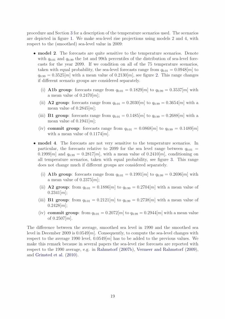
procedure and Section 3 for a description of the temperature scenarios used. The scenariosare depicted in figure 1. We make sea-level rise projections using models 2 and 4, withrespect to the (smoothed) sea-level value in 2009:

• model 2. The forecasts are quite sensitive to the temperature scenarios. Denotewith q0.01 and q0.99 the 1st and 99th percentiles of the distribution of sea-level fore-casts for the year 2099. If we condition on all of the 75 temperature scenarios,taken with equal probability, the sea-level forecasts range from q0.01 = 0.0948[m] toq0.99 = 0.3525[m] with a mean value of 0.2130[m], see figure 2. This range changesif different scenario groups are considered separately.

(i) A1b group: forecasts range from q0.01 = 0.1829[m] to q0.99 = 0.3537[m] witha mean value of 0.2470[m];

(ii) A2 group: forecasts range from q0.01 = 0.2030[m] to q0.99 = 0.3654[m] with amean value of 0.2845[m];

(iii) B1 group: forecasts range from q0.01 = 0.1485[m] to q0.99 = 0.2688[m] with amean value of 0.1941[m];

(iv) commit group: forecasts range from q0.01 = 0.0868[m] to q0.99 = 0.1489[m]with a mean value of 0.1174[m].

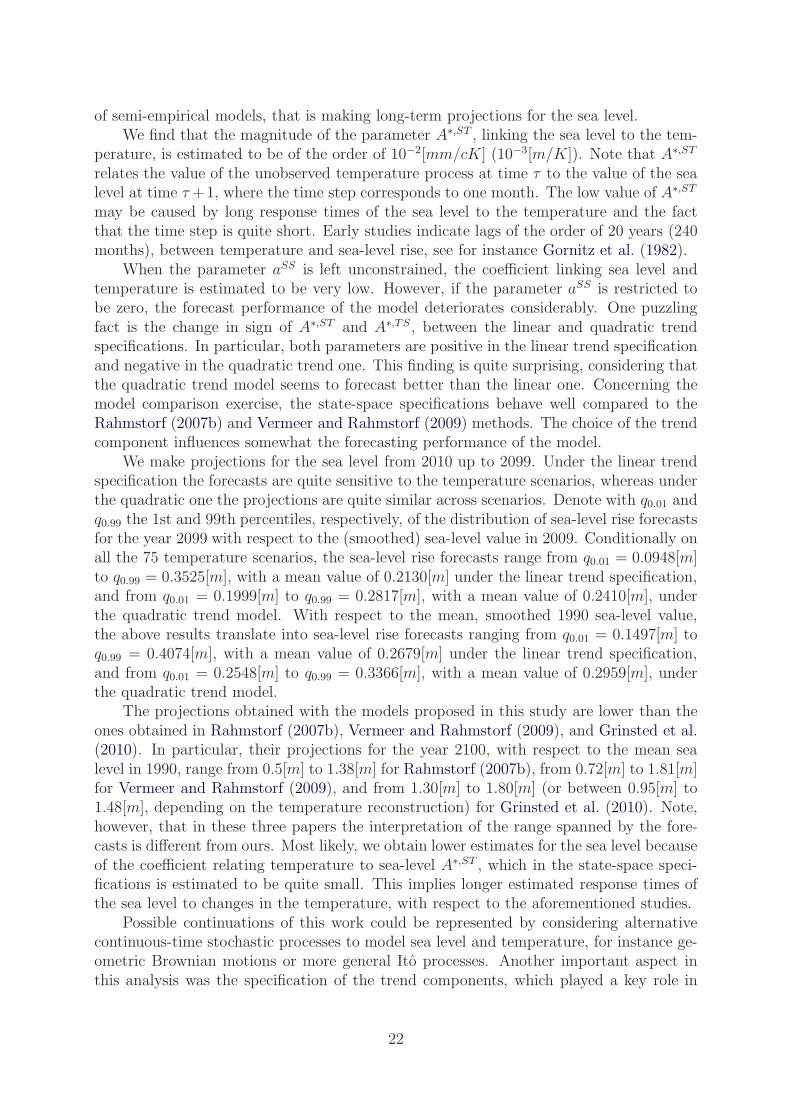
• model 4. The forecasts are not very sensitive to the temperature scenarios. Inparticular, the forecasts relative to 2099 for the sea level range between q0.01 =0.1999[m] and q0.99 = 0.2817[m], with a mean value of 0.2410[m], conditioning onall temperature scenarios, taken with equal probability, see figure 3. This rangedoes not change much if different groups are considered separately.

(i) A1b group: forecasts range from q0.01 = 0.1991[m] to q0.99 = 0.2696[m] witha mean value of 0.2375[m];

(ii) A2 group: from q0.01 = 0.1886[m] to q0.99 = 0.2704[m] with a mean value of0.2341[m];

(iii) B1 group: from q0.01 = 0.2121[m] to q0.99 = 0.2738[m] with a mean value of0.2428[m];

(iv) commit group: from q0.01 = 0.2072[m] to q0.99 = 0.2944[m] with a mean valueof 0.2507[m].

The difference between the average, smoothed sea level in 1990 and the smoothed sealevel in December 2009 is 0.0549[m]. Consequently, to compute the sea-level changes withrespect to the average 1990 level, 0.0549[m] has to be added to the previous values. Wemake this remark because in several papers the sea-level rise forecasts are reported withrespect to the 1990 average, e.g. in Rahmstorf (2007b), Vermeer and Rahmstorf (2009),and Grinsted et al. (2010).

19

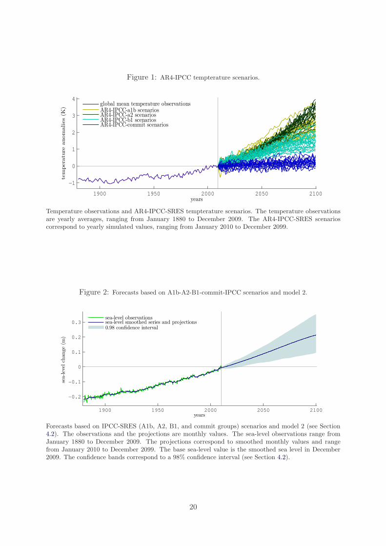
Figure 1: AR4-IPCC tempterature scenarios.

1900 1950 2000 2050 2100

−1

0

1

2

3

4

years

temperature

anomalies(K

)

global mean temperature observationsAR4-IPCC-a1b scenariosAR4-IPCC-a2 scenariosAR4-IPCC-b1 scenariosAR4-IPCC-commit scenarios

Temperature observations and AR4-IPCC-SRES tempterature scenarios. The temperature observationsare yearly averages, ranging from January 1880 to December 2009. The AR4-IPCC-SRES scenarioscorrespond to yearly simulated values, ranging from January 2010 to December 2099.

Figure 2: Forecasts based on A1b-A2-B1-commit-IPCC scenarios and model 2.

1900 1950 2000 2050 2100

−0.2

−0.1

0

0.1

0.2

0.3

years

sea-level

change(m

)

sea-level observationssea-level smoothed series and projections0.98 confidence interval

Forecasts based on IPCC-SRES (A1b, A2, B1, and commit groups) scenarios and model 2 (see Section4.2). The observations and the projections are monthly values. The sea-level observations range fromJanuary 1880 to December 2009. The projections correspond to smoothed monthly values and rangefrom January 2010 to December 2099. The base sea-level value is the smoothed sea level in December2009. The confidence bands correspond to a 98% confidence interval (see Section 4.2).

20

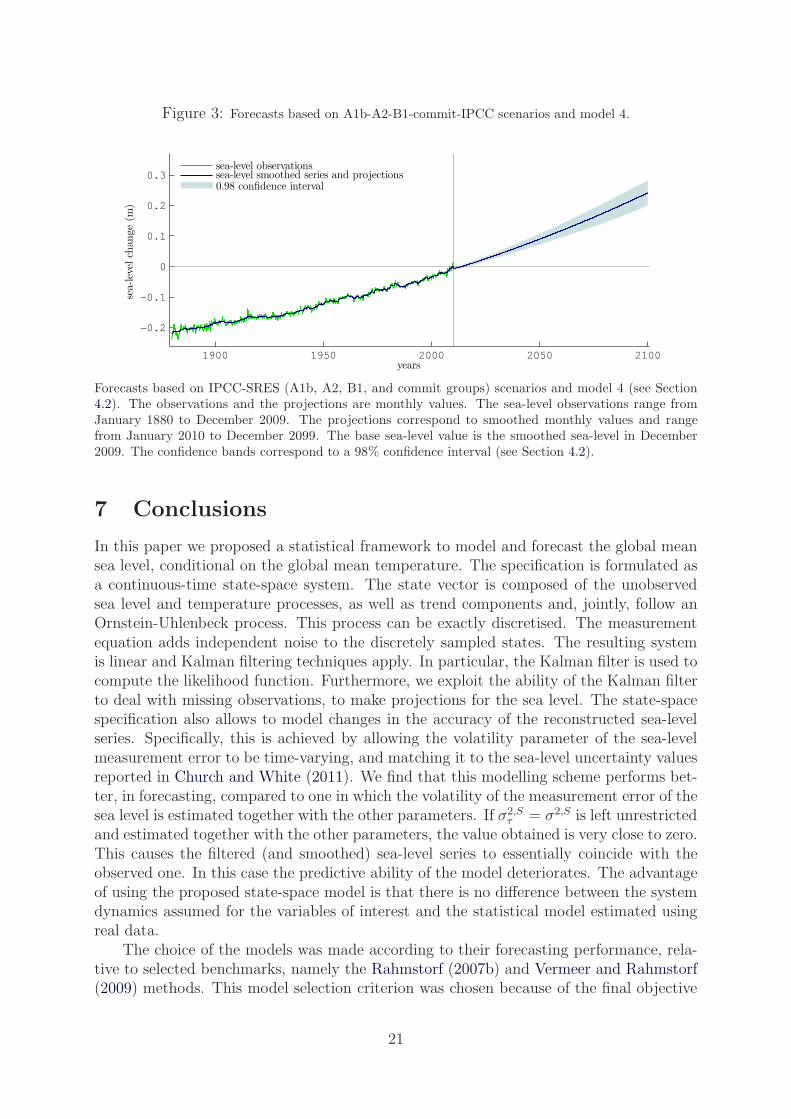
Figure 3: Forecasts based on A1b-A2-B1-commit-IPCC scenarios and model 4.

1900 1950 2000 2050 2100

−0.2

−0.1

0

0.1

0.2

0.3

years

sea-level

change(m

)

sea-level observationssea-level smoothed series and projections0.98 confidence interval

Forecasts based on IPCC-SRES (A1b, A2, B1, and commit groups) scenarios and model 4 (see Section4.2). The observations and the projections are monthly values. The sea-level observations range fromJanuary 1880 to December 2009. The projections correspond to smoothed monthly values and rangefrom January 2010 to December 2099. The base sea-level value is the smoothed sea-level in December2009. The confidence bands correspond to a 98% confidence interval (see Section 4.2).

7 Conclusions

In this paper we proposed a statistical framework to model and forecast the global meansea level, conditional on the global mean temperature. The specification is formulated asa continuous-time state-space system. The state vector is composed of the unobservedsea level and temperature processes, as well as trend components and, jointly, follow anOrnstein-Uhlenbeck process. This process can be exactly discretised. The measurementequation adds independent noise to the discretely sampled states. The resulting systemis linear and Kalman filtering techniques apply. In particular, the Kalman filter is used tocompute the likelihood function. Furthermore, we exploit the ability of the Kalman filterto deal with missing observations, to make projections for the sea level. The state-spacespecification also allows to model changes in the accuracy of the reconstructed sea-levelseries. Specifically, this is achieved by allowing the volatility parameter of the sea-levelmeasurement error to be time-varying, and matching it to the sea-level uncertainty valuesreported in Church and White (2011). We find that this modelling scheme performs bet-ter, in forecasting, compared to one in which the volatility of the measurement error of thesea level is estimated together with the other parameters. If σ2,S

τ = σ2,S is left unrestrictedand estimated together with the other parameters, the value obtained is very close to zero.This causes the filtered (and smoothed) sea-level series to essentially coincide with theobserved one. In this case the predictive ability of the model deteriorates. The advantageof using the proposed state-space model is that there is no difference between the systemdynamics assumed for the variables of interest and the statistical model estimated usingreal data.

The choice of the models was made according to their forecasting performance, rela-tive to selected benchmarks, namely the Rahmstorf (2007b) and Vermeer and Rahmstorf(2009) methods. This model selection criterion was chosen because of the final objective

21

of semi-empirical models, that is making long-term projections for the sea level.We find that the magnitude of the parameter A∗,ST , linking the sea level to the tem-

perature, is estimated to be of the order of 10−2[mm/cK] (10−3[m/K]). Note that A∗,ST

relates the value of the unobserved temperature process at time τ to the value of the sealevel at time τ +1, where the time step corresponds to one month. The low value of A∗,ST

may be caused by long response times of the sea level to the temperature and the factthat the time step is quite short. Early studies indicate lags of the order of 20 years (240months), between temperature and sea-level rise, see for instance Gornitz et al. (1982).

When the parameter aSS is left unconstrained, the coefficient linking sea level andtemperature is estimated to be very low. However, if the parameter aSS is restricted tobe zero, the forecast performance of the model deteriorates considerably. One puzzlingfact is the change in sign of A∗,ST and A∗,TS, between the linear and quadratic trendspecifications. In particular, both parameters are positive in the linear trend specificationand negative in the quadratic trend one. This finding is quite surprising, considering thatthe quadratic trend model seems to forecast better than the linear one. Concerning themodel comparison exercise, the state-space specifications behave well compared to theRahmstorf (2007b) and Vermeer and Rahmstorf (2009) methods. The choice of the trendcomponent influences somewhat the forecasting performance of the model.

We make projections for the sea level from 2010 up to 2099. Under the linear trendspecification the forecasts are quite sensitive to the temperature scenarios, whereas underthe quadratic one the projections are quite similar across scenarios. Denote with q0.01 andq0.99 the 1st and 99th percentiles, respectively, of the distribution of sea-level rise forecastsfor the year 2099 with respect to the (smoothed) sea-level value in 2009. Conditionally onall the 75 temperature scenarios, the sea-level rise forecasts range from q0.01 = 0.0948[m]to q0.99 = 0.3525[m], with a mean value of 0.2130[m] under the linear trend specification,and from q0.01 = 0.1999[m] to q0.99 = 0.2817[m], with a mean value of 0.2410[m], underthe quadratic trend model. With respect to the mean, smoothed 1990 sea-level value,the above results translate into sea-level rise forecasts ranging from q0.01 = 0.1497[m] toq0.99 = 0.4074[m], with a mean value of 0.2679[m] under the linear trend specification,and from q0.01 = 0.2548[m] to q0.99 = 0.3366[m], with a mean value of 0.2959[m], underthe quadratic trend model.

The projections obtained with the models proposed in this study are lower than theones obtained in Rahmstorf (2007b), Vermeer and Rahmstorf (2009), and Grinsted et al.(2010). In particular, their projections for the year 2100, with respect to the mean sealevel in 1990, range from 0.5[m] to 1.38[m] for Rahmstorf (2007b), from 0.72[m] to 1.81[m]for Vermeer and Rahmstorf (2009), and from 1.30[m] to 1.80[m] (or between 0.95[m] to1.48[m], depending on the temperature reconstruction) for Grinsted et al. (2010). Note,however, that in these three papers the interpretation of the range spanned by the fore-casts is different from ours. Most likely, we obtain lower estimates for the sea level becauseof the coefficient relating temperature to sea-level A∗,ST , which in the state-space speci-fications is estimated to be quite small. This implies longer estimated response times ofthe sea level to changes in the temperature, with respect to the aforementioned studies.

Possible continuations of this work could be represented by considering alternativecontinuous-time stochastic processes to model sea level and temperature, for instance ge-ometric Brownian motions or more general Ito processes. Another important aspect inthis analysis was the specification of the trend components, which played a key role in

22

the forecasting of the sea level. It would be interesting to study alternative specificationsfor the trend components and their relation to different climate forcings, such as humaninduced changes in greenhouse gases and aerosols concentrations.

23

References

Anthoff, D., R. J. Nicholls, and R. S. Tol (2010). The economic impact of substantialsea-level rise. Mitigation and Adaptation Strategies for Global Change 15 (4), 321–335.

Anthoff, D., R. J. Nicholls, R. S. Tol, and A. T. Vafeidis (2006). Global and regionalexposure to large rises in sea-level: a sensitivity analysis. Tyndall centre for climatechange research-Working Paper 96.

Arnell, N., E. L. Tompkins, N. Adger, and K. Delaney (2005). Vulnerability to abruptclimate change in europe.

Bergstrom, A. R. (1997). Gaussian estimation of mixed-order continuous-time dynamicmodels with unobservable stochastic trends from mixed stock and flow data. Econo-metric Theory 13 (04), 467–505.

Brockwell, P. J. and R. A. Davis (2009). Time series: theory and methods. Springer.

Budyko, M. I. (1968). On the origin of glacial epochs. Meteorol. Gidrol 2, 3–8.

Budyko, M. I. (1969). The effect of solar radiation variations on the climate of the earth.Tellus 21 (5), 611–619.

Budyko, M. I. (1972). The future climate. Eos, Transactions American GeophysicalUnion 53 (10), 868–874.

Cane, M. A., A. Kaplan, R. N. Miller, B. Tang, E. C. Hackert, and A. J. Busalacchi (1996).Mapping tropical pacific sea level: Data assimilation via a reduced state space kalmanfilter. Journal of Geophysical Research: Oceans (1978–2012) 101 (C10), 22599–22617.

Carter, T. (2007). General guidelines on the use of scenario data for climate impact andadaptation assessment. Technical report, Task Group on Data and Scenario Supportfor Impact and Climate Assessment (TGICA), Intergovernmental Panel on ClimateChange.

Cazenave, A. and R. S. Nerem (2004). Present-day sea level change: Observations andcauses. Reviews of Geophysics 42 (3).

Chan, N. H., J. B. Kadane, R. N. Miller, and W. Palma (1996). Estimation of tropical sealevel anomaly by an improved kalman filter. Journal of physical oceanography 26 (7),1286–1303.

Church, J. A. and N. J. White (2006). A 20th century acceleration in global sea-level rise.Geophysical research letters 33 (1).

Church, J. A. and N. J. White (2011). Sea-level rise from the late 19th to the early 21stcentury. Surveys in Geophysics 32 (4-5), 585–602.

Durbin, J. and S. J. Koopman (2012). Time series analysis by state space methods. OxfordUniversity Press.

Fraedrich, K. (1978). Structural and stochastic analysis of a zero-dimensional climatesystem. Quarterly Journal of the Royal Meteorological Society 104 (440), 461–474.

Gornitz, V., S. Lebedeff, and J. Hansen (1982). Global sea level trend in the past century.Science 215 (4540), 1611–1614.

Grinsted, A., J. C. Moore, and S. Jevrejeva (2010). Reconstructing sea level from paleoand projected temperatures 200 to 2100 ad. Climate Dynamics 34 (4), 461–472.

Hansen, J., R. Ruedy, M. Sato, M. Imhoff, W. Lawrence, D. Easterling, T. Peterson, andT. Karl (2001). A closer look at united states and global surface temperature change.Journal of Geophysical Research: Atmospheres (1984–2012) 106 (D20), 23947–23963.

Hansen, J., R. Ruedy, M. Sato, and K. Lo (2010). Global surface temperature change.Reviews of Geophysics 48 (4).

Hansen, N. and A. Ostermeier (1996). Adapting arbitrary normal mutation distributionsin evolution strategies: The covariance matrix adaptation. In Evolutionary Computa-tion, 1996., Proceedings of IEEE International Conference on, pp. 312–317. IEEE.

Harvey, A. and J. H. Stock (1993). Estimation, smoothing, interpolation, and distributionfor structural time-series models in continuous time. Models, Methods and Applicationsof Econometrics , 55–70.

Hasselmann, K. (1976). Stochastic climate models part i. theory. Tellus 28 (6), 473–485.

Hay, C. C., E. Morrow, R. E. Kopp, and J. X. Mitrovica (2013). Estimating the sourcesof global sea level rise with data assimilation techniques. Proceedings of the NationalAcademy of Sciences 110 (Supplement 1), 3692–3699.

Holgate, S., S. Jevrejeva, P. Woodworth, and S. Brewer (2007). Comment on “a semi-empirical approach to projecting future sea-level rise”. Science 317 (5846), 1866–1866.

Imkeller, P. (2001). Energy balance modelsviewed from stochastic dynamics. In Stochasticclimate models, pp. 213–240. Springer.

Jevrejeva, S., A. Grinsted, and J. Moore (2009). Anthropogenic forcing dominates sealevel rise since 1850. Geophysical Research Letters 36 (20).

Jevrejeva, S., J. Moore, and A. Grinsted (2010). How will sea level respond to changes innatural and anthropogenic forcings by 2100? Geophysical research letters 37 (7).

Jevrejeva, S., J. C. Moore, and A. Grinsted (2012a). Potential for bias in 21st centurysemiempirical sea level projections. Journal of Geophysical Research: Atmospheres(1984–2012) 117 (D20).

Jevrejeva, S., J. C. Moore, and A. Grinsted (2012b). Sea level projections to ad2500 witha new generation of climate change scenarios. Global and Planetary Change 80, 14–20.

Kemp, A. C., B. P. Horton, J. P. Donnelly, M. E. Mann, M. Vermeer, and S. Rahmstorf(2011). Climate related sea-level variations over the past two millennia. Proceedings ofthe National Academy of Sciences .

Koopman, S. J. and J. Durbin (2000). Fast filtering and smoothing for multivariate statespace models. Journal of Time Series Analysis 21 (3), 281–296.

Liu, R. Y. et al. (1988). Bootstrap procedures under some non-iid models. The Annalsof Statistics 16 (4), 1696–1708.

Mammen, E. (1993). Bootstrap and wild bootstrap for high dimensional linear models.The Annals of Statistics , 255–285.

Meehl, G. A., C. Covey, K. E. Taylor, T. Delworth, R. J. Stouffer, M. Latif, B. McAvaney,and J. F. Mitchell (2007). The wcrp cmip3 multimodel dataset: A new era in climatechange research. Bulletin of the American Meteorological Society 88 (9), 1383–1394.

Meehl, G. A., T. F. Stocker, W. D. Collins, P. Friedlingstein, A. T. Gaye, J. M. Gregory,A. Kitoh, R. Knutti, J. M. Murphy, A. Noda, et al. (2007). Global climate projections.Climate change 283.

Miller, R. N. and M. A. Cane (1989). A kalman filter analysis of sea level height in thetropical pacific.

Moore, J. C., A. Grinsted, T. Zwinger, and S. Jevrejeva (2013). Semiempirical andprocess-based global sea level projections. Reviews of Geophysics 51 (3), 484–522.

Munk, W. (2002). Twentieth century sea level: An enigma. Proceedings of the nationalacademy of sciences 99 (10), 6550–6555.

Nicolis, C. (1982). Stochastic aspects of climatic transitionsresponse to a periodic forcing.Tellus 34 (1), 1–9.

North, G. R., R. F. Cahalan, and J. A. Coakley (1981). Energy balance climate models.Reviews of Geophysics 19 (1), 91–121.

Pardaens, A., J. Lowe, S. Brown, R. Nicholls, and D. De Gusmao (2011). Sea-level riseand impacts projections under a future scenario with large greenhouse gas emissionreductions. Geophysical Research Letters 38 (12).

Press, W. H., S. A. Teukolsky, W. T. Vetterling, and B. P. Flannery (2002). NumericalRecipes in C++ (Second ed.). Cambridge University Press, Cambridge.

Pretis, F. (2015). Econometric methods to model non-stationary climate systems: theequivalence of two-component energy balance models and cointegrated VARs. Technicalreport, Institute for new economic thinking, Oxfor Martin School, University of Oxford.

Rahmstorf, S. (2007a). Response to comments on “a semi-empirical approach to projectingfuture sea-level rise”. Science 317 (5846), 1866d–1866d.

Rahmstorf, S. (2007b). A semi-empirical approach to projecting future sea-level rise.Science 315 (5810), 368–370.

Rodriguez, A. and E. Ruiz (2009). Bootstrap prediction intervals in state–space models.Journal of time series analysis 30 (2), 167–178.

Sellers, W. D. (1969). A global climatic model based on the energy balance of the earth-atmosphere system. Journal of Applied Meteorology 8 (3), 392–400.

Solomon, S., G.-K. Plattner, R. Knutti, and P. Friedlingstein (2009). Irreversible cli-mate change due to carbon dioxide emissions. Proceedings of the national academy ofsciences 106 (6), 1704–1709.

Sugiyama, M., R. J. Nicholls, and A. Vafeidis (2008). Estimating the economic cost ofsea-level rise. Technical report, MIT Joint Program on the Science and Policy of GlobalChange.

Vermeer, M. and S. Rahmstorf (2009). Global sea level linked to global temperature.Proceedings of the National Academy of Sciences 106 (51), 21527–21532.

Wu, C.-F. J. (1986). Jackknife, bootstrap and other resampling methods in regressionanalysis. the Annals of Statistics , 1261–1295.

Appendices

A Details of univariate Kalman filter

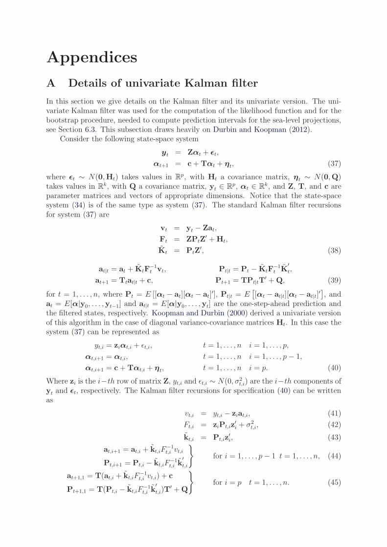
In this section we give details on the Kalman filter and its univariate version. The uni-variate Kalman filter was used for the computation of the likelihood function and for thebootstrap procedure, needed to compute prediction intervals for the sea-level projections,see Section 6.3. This subsection draws heavily on Durbin and Koopman (2012).

Consider the following state-space system

yt = Zαt + ǫt,

αt+1 = c+Tαt + ηt, (37)

where ǫt ∼ N(0,Ht) takes values in Rp, with Ht a covariance matrix, ηt ∼ N(0,Q)

takes values in Rk, with Q a covariance matrix, yt ∈ R

p, αt ∈ Rk, and Z, T, and c are

parameter matrices and vectors of appropriate dimensions. Notice that the state-spacesystem (34) is of the same type as system (37). The standard Kalman filter recursionsfor system (37) are

vt = yt − Zat,

Ft = ZPtZ′ +Ht,

Kt = PtZ′, (38)

at|t = at + KtF−1t vt, Pt|t = Pt − KtF

−1t K

′t,

at+1 = Ttat|t + c, Pt+1 = TPt|tT′ +Q, (39)

for t = 1, . . . , n, where Pt = E [[αt − at][αt − at]′], Pt|t = E

[[αt − at|t][αt − at|t]

′], andat = E[α|y0, . . . ,yt−1] and at|t = E[α|y0, . . . ,yt] are the one-step-ahead prediction andthe filtered states, respectively. Koopman and Durbin (2000) derived a univariate versionof this algorithm in the case of diagonal variance-covariance matrices Ht. In this case thesystem (37) can be represented as

yt,i = ziαt,i + ǫt,i, t = 1, . . . , n i = 1, . . . , p,

αt,i+1 = αt,i, t = 1, . . . , n i = 1, . . . , p− 1,

αt,i+1 = c+Tαt,i + ηt, t = 1, . . . , n i = p. (40)

Where zi is the i−th row of matrix Z, yt,i and ǫt,i ∼ N(0, σ2t,i) are the i−th components of

yt and ǫt, respectively. The Kalman filter recursions for specification (40) can be writtenas

vt,i = yt,i − ziat,i, (41)

Ft,i = ziPt,iz′i + σ2

t,i, (42)

kt,i = Pt,iz′i, (43)

at,i+1 = at,i + kt,iF−1t,i vt,i

Pt,i+1 = Pt,i − kt,iF−1t,i k

′t,i

}

for i = 1, . . . , p− 1 t = 1, . . . , n, (44)

at+1,1 = T(at,i + kt,iF−1t,i vt,i) + c

Pt+1,1 = T(Pt,i − kt,iF−1t,i k

′t,i)T

′ +Q

}

for i = p t = 1, . . . , n. (45)

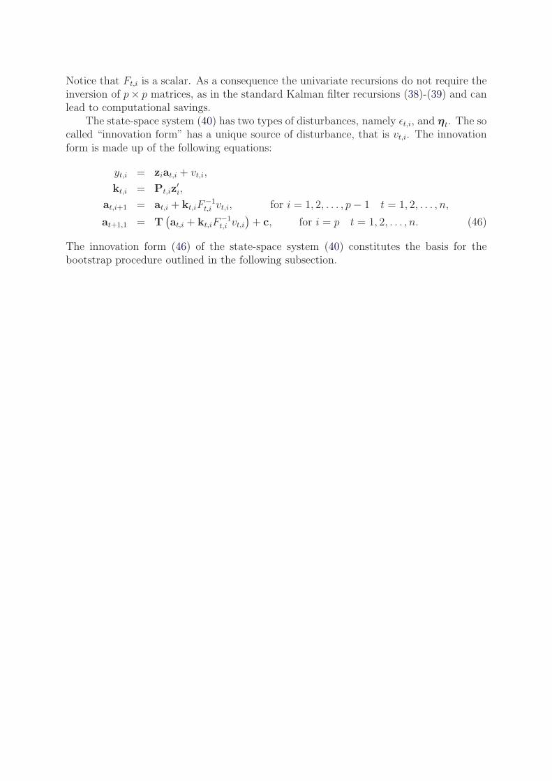
Notice that Ft,i is a scalar. As a consequence the univariate recursions do not require theinversion of p× p matrices, as in the standard Kalman filter recursions (38)-(39) and canlead to computational savings.

The state-space system (40) has two types of disturbances, namely ǫt,i, and ηt. The socalled “innovation form” has a unique source of disturbance, that is vt,i. The innovationform is made up of the following equations:

yt,i = ziat,i + vt,i,

kt,i = Pt,iz′i,

at,i+1 = at,i + kt,iF−1t,i vt,i, for i = 1, 2, . . . , p− 1 t = 1, 2, . . . , n,

at+1,1 = T(at,i + kt,iF

−1t,i vt,i

)+ c, for i = p t = 1, 2, . . . , n. (46)

The innovation form (46) of the state-space system (40) constitutes the basis for thebootstrap procedure outlined in the following subsection.

B Bootstrap procedure

In this section we outline the bootstrap procedure used to compute the prediction intervalsfor the sea-level projections, conditional on the IPCC scenarios, as described in Section 6.3.We detail the algorithm with respect to the state-space system (37) and the Kalman filterrecursions (41)-(45). The algorithm is a modification of the one proposed in Rodriguezand Ruiz (2009) that allows for time-varying measurement error variances. Denote withθ the vector containing the parameters of the state-space system (37). The algorithm wepropose is made up of the following steps:

1. estimate the parameters of model (30) by maximum likelihood and obtain θ andthe sequence of innovations {vt,i}i=1,...,p

t=1,...,n;

2. compute the centred innovations {vct,i}i=1,...,pt=1,...,n, obtained as vct,i = vt,i − vn,i, with

vn,i = (1/n)∑n

t=1 vt,i;

3. obtain the standardized innovations {vst,i}i=1,...,pt=1,...,n, computed as vst,i =

vct,i√Ft,i

;

4. obtain a sequence of bootstrap standardized innovations {v∗t,i}i=1,...,pt=1,...,n via random

draws with replacement from the randomly scaled standardized innovations {vst,i ·ǫt,i}i=1,...,p

t=1,...,n, where ǫt,i ∼ N(0, 1);

5. compute a bootstrap replicate of the observations {y∗t,i}i=1,...,pt=1,...,n by means of the in-

novation form (46) using {v∗t,i}i=1,...,pt=1,...,n and the estimated parameters θ;

6. estimate the corresponding bootstrap parameters θ∗from the bootstrap replicates;

7. run the Kalman filter with θ∗using the original observations and one temperature

scenario as described in Section 4.2.

Steps 1-7 are repeated N = 500 for each temperature scenario. As made clear in step 4 wemake use of a wild bootstrap procedure as opposed to the simple re-sampling method usedin Rodriguez and Ruiz (2009). The wild bootstrap was originally proposed by Wu (1986)and it is well known in the literature to perform better than a simple resampling scheme inthe presence of heteroskedasticity, see for instance Liu et al. (1988) and Mammen (1993).In this paper the heteroskedasticity comes from the time varying matrixHt. Note that thevariance of the innovations vt,i is given by Ft,i = ziPt,iz

′i + σ2

t,i where σ2t,i is time-varying.

In the notation of equation (33), it’s the parameter σ2,St that causes the innovations vt,i,

in equation (41), to be heteroskedastic.

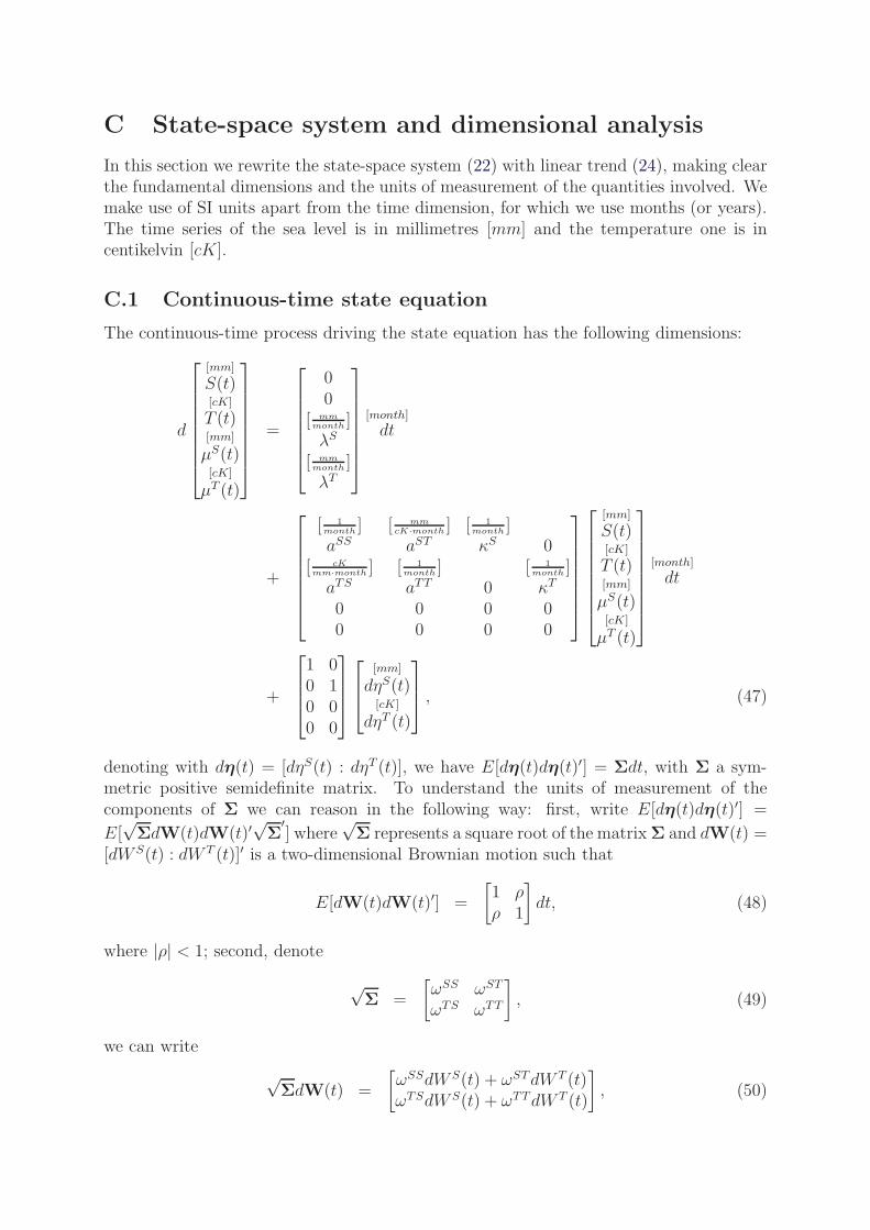
C State-space system and dimensional analysis

In this section we rewrite the state-space system (22) with linear trend (24), making clearthe fundamental dimensions and the units of measurement of the quantities involved. Wemake use of SI units apart from the time dimension, for which we use months (or years).The time series of the sea level is in millimetres [mm] and the temperature one is incentikelvin [cK].

C.1 Continuous-time state equation

The continuous-time process driving the state equation has the following dimensions:

d

[mm]

S(t)[cK]

T (t)[mm]

µS(t)[cK]

µT (t)

=

00

[ mmmonth ]λS

[ mmmonth ]λT

[month]

dt

+

[ 1

month ]aSS

[ mmcK·month ]aST

[ 1

month ]κS 0

[ cKmm·month ]aTS

[ 1

month ]aTT 0

[ 1

month ]κT

0 0 0 00 0 0 0

[mm]

S(t)[cK]

T (t)[mm]

µS(t)[cK]

µT (t)

[month]

dt

+

1 00 10 00 0

[mm]

dηS(t)[cK]

dηT (t)

, (47)

denoting with dη(t) = [dηS(t) : dηT (t)], we have E[dη(t)dη(t)′] = Σdt, with Σ a sym-metric positive semidefinite matrix. To understand the units of measurement of thecomponents of Σ we can reason in the following way: first, write E[dη(t)dη(t)′] =

E[√ΣdW(t)dW(t)′

√Σ

′] where

√Σ represents a square root of the matrixΣ and dW(t) =

[dW S(t) : dW T (t)]′ is a two-dimensional Brownian motion such that

E[dW(t)dW(t)′] =

[1 ρρ 1

]

dt, (48)

where |ρ| < 1; second, denote

√Σ =

[ωSS ωST

ωTS ωTT

]

, (49)

we can write

√ΣdW(t) =

[ωSSdW S(t) + ωSTdW T (t)ωTSdW S(t) + ωTTdW T (t)

]

, (50)

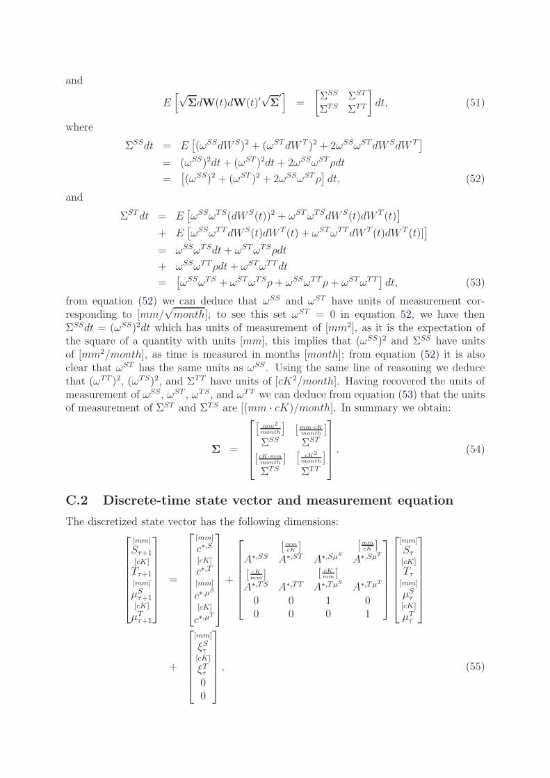
and

E[√

ΣdW(t)dW(t)′√Σ

′]=

[ΣSS ΣST

ΣTS ΣTT

]

dt, (51)

where

ΣSSdt = E[(ωSSdW S)2 + (ωSTdW T )2 + 2ωSSωSTdW SdW T

]

= (ωSS)2dt+ (ωST )2dt+ 2ωSSωSTρdt

=[(ωSS)2 + (ωST )2 + 2ωSSωSTρ

]dt, (52)

and

ΣSTdt = E[ωSSωTS(dW S(t))2 + ωSTωTSdW S(t)dW T (t)

]

+ E[ωSSωTTdW S(t)dW T (t) + ωSTωTTdW T (t)dW T (t)]

]

= ωSSωTSdt+ ωSTωTSρdt

+ ωSSωTTρdt+ ωSTωTTdt

=[ωSSωTS + ωSTωTSρ+ ωSSωTTρ+ ωSTωTT

]dt, (53)

from equation (52) we can deduce that ωSS and ωST have units of measurement cor-responding to [mm/

√month]; to see this set ωST = 0 in equation 52, we have then

ΣSSdt = (ωSS)2dt which has units of measurement of [mm2], as it is the expectation ofthe square of a quantity with units [mm], this implies that (ωSS)2 and ΣSS have unitsof [mm2/month], as time is measured in months [month]; from equation (52) it is alsoclear that ωST has the same units as ωSS. Using the same line of reasoning we deducethat (ωTT )2, (ωTS)2, and ΣTT have units of [cK2/month]. Having recovered the units ofmeasurement of ωSS, ωST , ωTS, and ωTT we can deduce from equation (53) that the unitsof measurement of ΣST and ΣTS are [(mm · cK)/month]. In summary we obtain:

Σ =

[

mm2

month

]

ΣSS

[mm·cKmonth ]ΣST

[ cK·mmmonth ]ΣTS

[

cK2

month

]

ΣTT

. (54)

C.2 Discrete-time state vector and measurement equation

The discretized state vector has the following dimensions:

[mm]

Sτ+1[cK]

Tτ+1[mm]

µSτ+1[cK]

µTτ+1

=

[mm]

c∗,S

[cK]

c∗,T

[mm]

c∗,µS

[cK]

c∗,µT

+

A∗,SS[mm

cK ]A∗,ST A∗,SµS

[mmcK ]

A∗,SµT

[ cKmm ]

A∗,TS A∗,TT

[ cKmm ]

A∗,TµS

A∗,TµT

0 0 1 00 0 0 1

[mm]

Sτ

[cK]

Tτ

[mm]

µSτ

[cK]

µTτ

+

[mm]

ξSτ[cK]

ξTτ00

, (55)

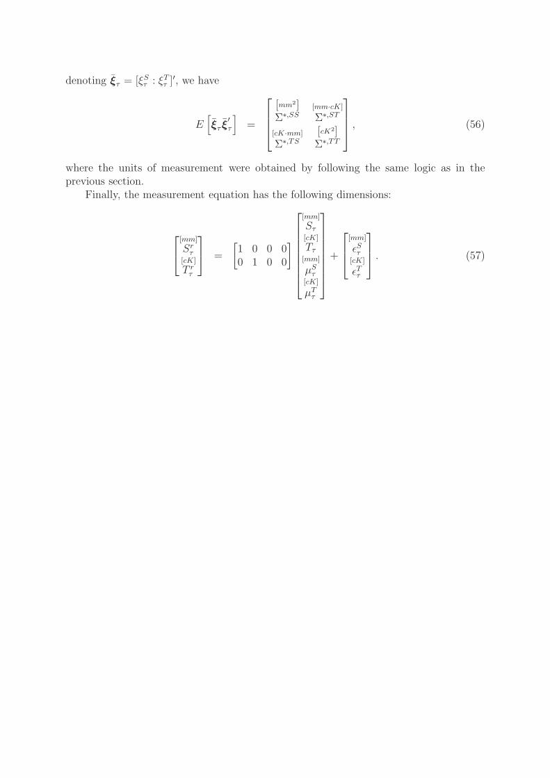
denoting ξτ = [ξSτ : ξTτ ]′, we have

E[

ξτ ξ′τ

]

=

[mm2]Σ∗,SS

[mm·cK]

Σ∗,ST

[cK·mm]

Σ∗,TS

[cK2]Σ∗,TT

, (56)

where the units of measurement were obtained by following the same logic as in theprevious section.

Finally, the measurement equation has the following dimensions:

[mm]

Srτ

[cK]

T rτ

=

[1 0 0 00 1 0 0

]

[mm]

Sτ

[cK]

Tτ

[mm]

µSτ

[cK]

µTτ

+

[mm]

ǫSτ[cK]

ǫTτ

. (57)

D Tables

In this section we report the tables with the results for the model comparison forecastingexercise and the parameter estimates for models 1-2 and models 3-4. See Sections 4 and6 for more details.

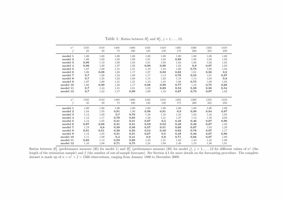
Table 1: Ratios between R1

f and Rjf , j = 1, . . . , 12.

n∗ 1535 1510 1485 1460 1435 1410 1385 1360 1335 1310f 25 50 75 100 125 150 175 200 225 250

model 1 1,00 1,00 1,00 1,00 1,00 1,00 1,00 1,00 1,00 1,00model 2 1,00 1,02 1,02 1,00 1,01 1,04 0,89 1,06 1,03 1,02model 3 0,99 1,10 1,08 1,03 1,01 1,03 1,02 1,00 1,02 1,03model 4 0,99 1,09 1,07 1,02 0,99 0,99 1,02 0,9 0,97 1,03model 5 1,07 1,00 1,31 1,21 1,19 1,24 1,06 0,75 1,09 1,04model 6 1,06 0,98 1,26 1,17 1,07 0,82 0,62 1,01 0,56 0,5

model 7 0,7 1,26 1,24 1,09 1,17 1,14 0,76 0,55 1,01 0,97

model 8 0,7 1,25 1,22 1,08 1,15 1,22 1,19 1,15 1,03 0,9

model 9 1,07 1,00 1,31 1,21 1,19 1,24 1,06 0,75 1,09 1,04model 10 1,06 0,99 1,26 1,17 0,98 0,99 0,77 1,16 0,75 0,66

model 11 0,7 1,24 1,21 1,01 1,02 0,89 0,52 0,38 0,56 0,54

model 12 0,7 1,22 1,17 0,99 1,00 1,18 0,87 0,73 0,97 1,02

n∗ 1535 1510 1485 1460 1435 1410 1385 1360 1335 1310f 25 50 75 100 125 150 175 200 225 250

model 1 1,00 1,00 1,00 1,00 1,00 1,00 1,00 1,00 1,00 1,00model 2 1,04 1,05 0,91 1,00 0,98 0,91 0,9 0,99 0,94 0,97

model 3 1,14 1,09 0,7 0,76 1,28 1,10 1,23 1,04 1,42 1,85model 4 1,12 1,17 0,78 0,85 1,36 1,21 1,37 1,12 1,59 2,03model 5 1,12 1,05 0,31 0,31 0,67 0,5 0,48 0,46 0,67 0,96

model 6 0,87 0,68 0,31 0,31 0,59 0,52 0,49 0,46 0,67 1,02model 7 1,19 0,6 0,38 0,36 0,57 0,51 0,68 0,87 1,03 1,29model 8 0,91 0,51 0,38 0,35 0,54 0,48 0,62 0,78 0,97 1,17model 9 1,12 1,05 0,31 0,31 0,67 0,5 0,48 0,46 0,67 0,96

model 10 1,11 1,09 0,4 0,41 0,9 0,8 0,71 0,66 0,97 1,89model 11 0,85 1,14 0,59 0,66 1,23 1,21 1,63 1,43 1,42 1,80model 12 1,10 1,08 0,71 0,75 1,24 1,09 1,48 1,53 1,36 1,91

Ratios between R1

f (performance measure (35) for model 1) and Rjf (performance measure (35) for model j), j = 1, . . . , 12 for different values of n∗ (the

length of the estimation sample) and f (the number of out-of-sample forecasts). See Section 4.1 for more details on the forecasting procedure. The completedataset is made up of n = n∗ + f = 1560 observations, ranging from January 1880 to December 2009.

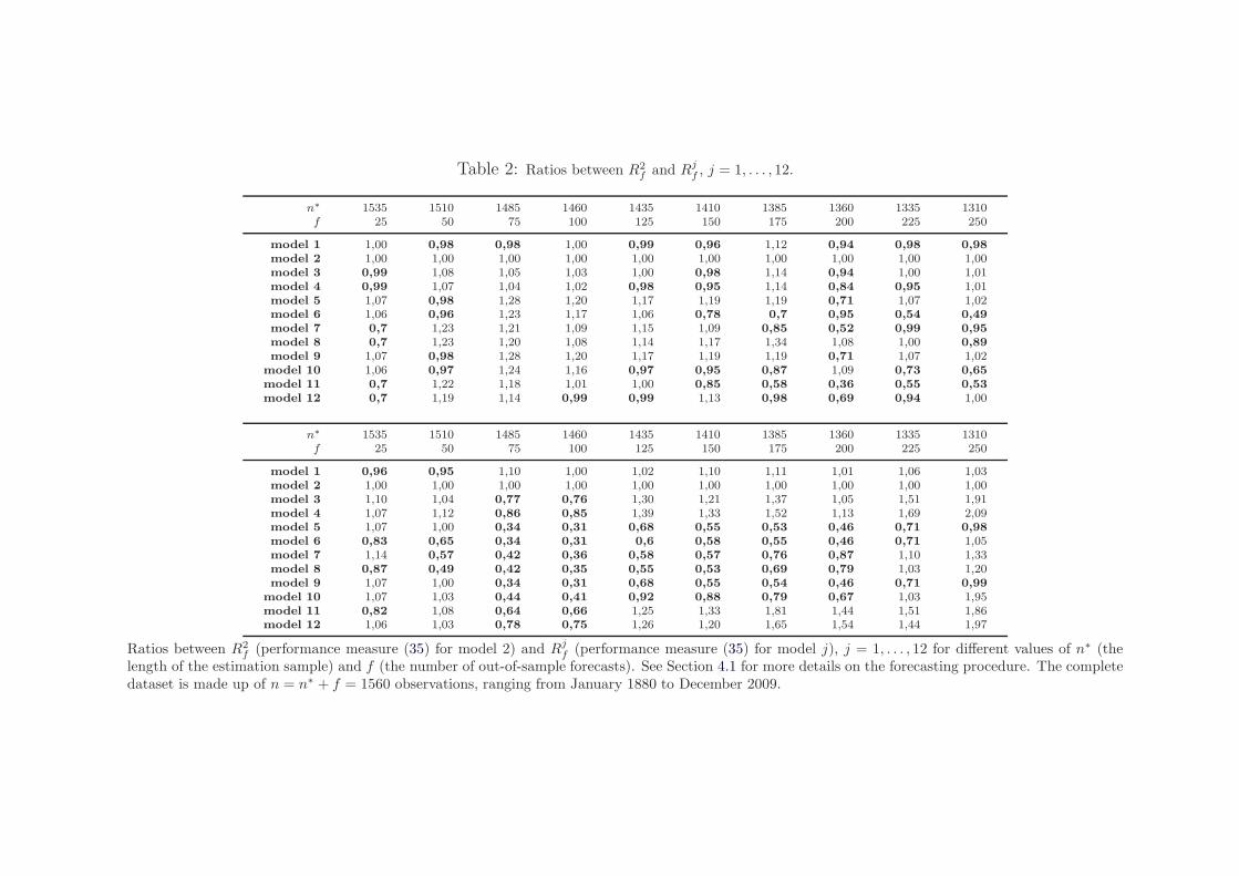
Table 2: Ratios between R2

f and Rjf , j = 1, . . . , 12.

n∗ 1535 1510 1485 1460 1435 1410 1385 1360 1335 1310f 25 50 75 100 125 150 175 200 225 250

model 1 1,00 0,98 0,98 1,00 0,99 0,96 1,12 0,94 0,98 0,98

model 2 1,00 1,00 1,00 1,00 1,00 1,00 1,00 1,00 1,00 1,00model 3 0,99 1,08 1,05 1,03 1,00 0,98 1,14 0,94 1,00 1,01model 4 0,99 1,07 1,04 1,02 0,98 0,95 1,14 0,84 0,95 1,01model 5 1,07 0,98 1,28 1,20 1,17 1,19 1,19 0,71 1,07 1,02model 6 1,06 0,96 1,23 1,17 1,06 0,78 0,7 0,95 0,54 0,49

model 7 0,7 1,23 1,21 1,09 1,15 1,09 0,85 0,52 0,99 0,95

model 8 0,7 1,23 1,20 1,08 1,14 1,17 1,34 1,08 1,00 0,89

model 9 1,07 0,98 1,28 1,20 1,17 1,19 1,19 0,71 1,07 1,02model 10 1,06 0,97 1,24 1,16 0,97 0,95 0,87 1,09 0,73 0,65

model 11 0,7 1,22 1,18 1,01 1,00 0,85 0,58 0,36 0,55 0,53

model 12 0,7 1,19 1,14 0,99 0,99 1,13 0,98 0,69 0,94 1,00

n∗ 1535 1510 1485 1460 1435 1410 1385 1360 1335 1310f 25 50 75 100 125 150 175 200 225 250

model 1 0,96 0,95 1,10 1,00 1,02 1,10 1,11 1,01 1,06 1,03model 2 1,00 1,00 1,00 1,00 1,00 1,00 1,00 1,00 1,00 1,00model 3 1,10 1,04 0,77 0,76 1,30 1,21 1,37 1,05 1,51 1,91model 4 1,07 1,12 0,86 0,85 1,39 1,33 1,52 1,13 1,69 2,09model 5 1,07 1,00 0,34 0,31 0,68 0,55 0,53 0,46 0,71 0,98

model 6 0,83 0,65 0,34 0,31 0,6 0,58 0,55 0,46 0,71 1,05model 7 1,14 0,57 0,42 0,36 0,58 0,57 0,76 0,87 1,10 1,33model 8 0,87 0,49 0,42 0,35 0,55 0,53 0,69 0,79 1,03 1,20model 9 1,07 1,00 0,34 0,31 0,68 0,55 0,54 0,46 0,71 0,99

model 10 1,07 1,03 0,44 0,41 0,92 0,88 0,79 0,67 1,03 1,95model 11 0,82 1,08 0,64 0,66 1,25 1,33 1,81 1,44 1,51 1,86model 12 1,06 1,03 0,78 0,75 1,26 1,20 1,65 1,54 1,44 1,97

Ratios between R2

f (performance measure (35) for model 2) and Rjf (performance measure (35) for model j), j = 1, . . . , 12 for different values of n∗ (the

length of the estimation sample) and f (the number of out-of-sample forecasts). See Section 4.1 for more details on the forecasting procedure. The completedataset is made up of n = n∗ + f = 1560 observations, ranging from January 1880 to December 2009.

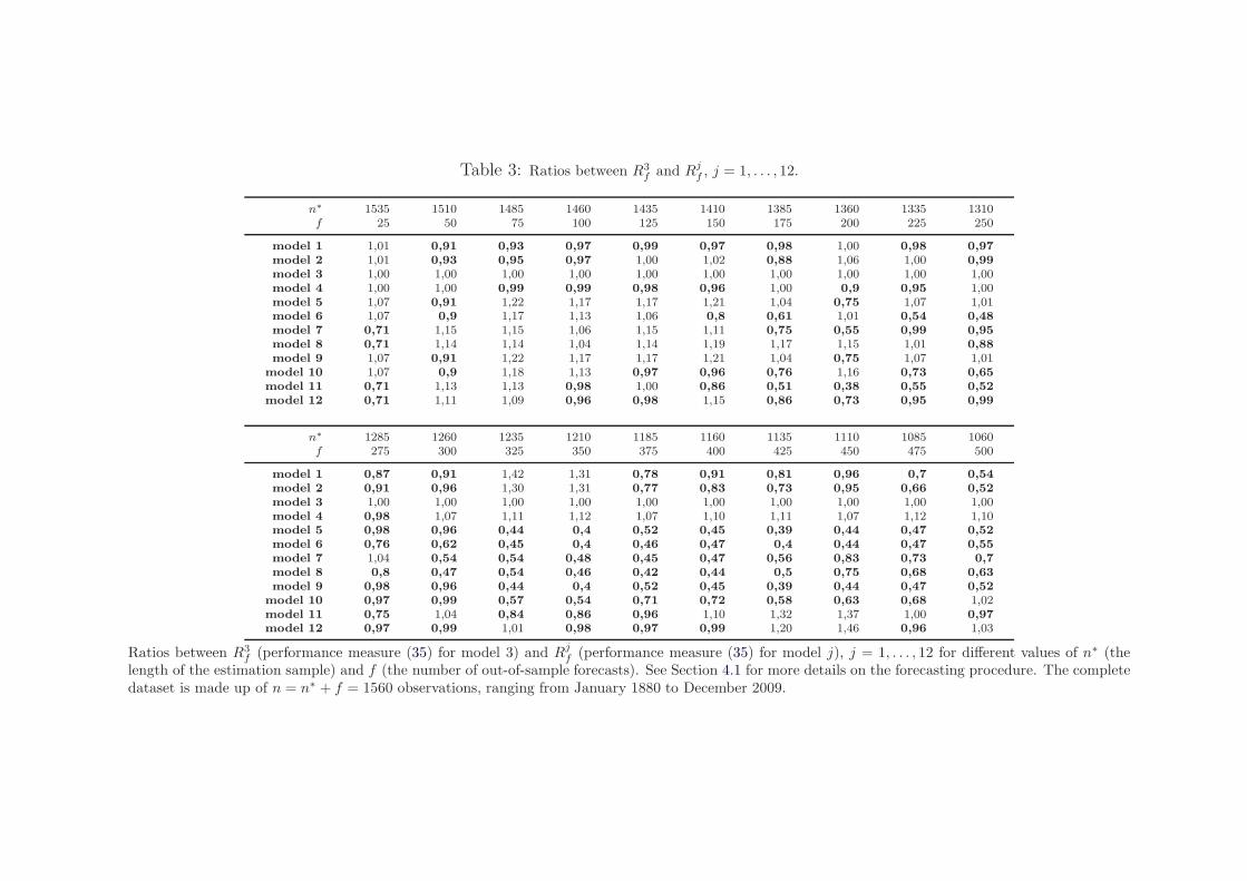
Table 3: Ratios between R3

f and Rjf , j = 1, . . . , 12.

n∗ 1535 1510 1485 1460 1435 1410 1385 1360 1335 1310f 25 50 75 100 125 150 175 200 225 250

model 1 1,01 0,91 0,93 0,97 0,99 0,97 0,98 1,00 0,98 0,97

model 2 1,01 0,93 0,95 0,97 1,00 1,02 0,88 1,06 1,00 0,99

model 3 1,00 1,00 1,00 1,00 1,00 1,00 1,00 1,00 1,00 1,00model 4 1,00 1,00 0,99 0,99 0,98 0,96 1,00 0,9 0,95 1,00model 5 1,07 0,91 1,22 1,17 1,17 1,21 1,04 0,75 1,07 1,01model 6 1,07 0,9 1,17 1,13 1,06 0,8 0,61 1,01 0,54 0,48

model 7 0,71 1,15 1,15 1,06 1,15 1,11 0,75 0,55 0,99 0,95

model 8 0,71 1,14 1,14 1,04 1,14 1,19 1,17 1,15 1,01 0,88

model 9 1,07 0,91 1,22 1,17 1,17 1,21 1,04 0,75 1,07 1,01model 10 1,07 0,9 1,18 1,13 0,97 0,96 0,76 1,16 0,73 0,65

model 11 0,71 1,13 1,13 0,98 1,00 0,86 0,51 0,38 0,55 0,52

model 12 0,71 1,11 1,09 0,96 0,98 1,15 0,86 0,73 0,95 0,99

n∗ 1285 1260 1235 1210 1185 1160 1135 1110 1085 1060f 275 300 325 350 375 400 425 450 475 500

model 1 0,87 0,91 1,42 1,31 0,78 0,91 0,81 0,96 0,7 0,54

model 2 0,91 0,96 1,30 1,31 0,77 0,83 0,73 0,95 0,66 0,52

model 3 1,00 1,00 1,00 1,00 1,00 1,00 1,00 1,00 1,00 1,00model 4 0,98 1,07 1,11 1,12 1,07 1,10 1,11 1,07 1,12 1,10model 5 0,98 0,96 0,44 0,4 0,52 0,45 0,39 0,44 0,47 0,52

model 6 0,76 0,62 0,45 0,4 0,46 0,47 0,4 0,44 0,47 0,55

model 7 1,04 0,54 0,54 0,48 0,45 0,47 0,56 0,83 0,73 0,7

model 8 0,8 0,47 0,54 0,46 0,42 0,44 0,5 0,75 0,68 0,63

model 9 0,98 0,96 0,44 0,4 0,52 0,45 0,39 0,44 0,47 0,52

model 10 0,97 0,99 0,57 0,54 0,71 0,72 0,58 0,63 0,68 1,02model 11 0,75 1,04 0,84 0,86 0,96 1,10 1,32 1,37 1,00 0,97

model 12 0,97 0,99 1,01 0,98 0,97 0,99 1,20 1,46 0,96 1,03

Ratios between R3

f (performance measure (35) for model 3) and Rjf (performance measure (35) for model j), j = 1, . . . , 12 for different values of n∗ (the

length of the estimation sample) and f (the number of out-of-sample forecasts). See Section 4.1 for more details on the forecasting procedure. The completedataset is made up of n = n∗ + f = 1560 observations, ranging from January 1880 to December 2009.

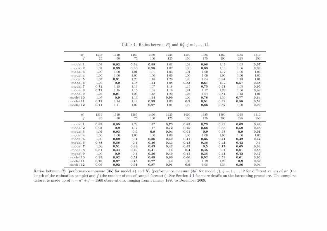
Table 4: Ratios between R4

f and Rjf , j = 1, . . . , 12.

n∗ 1535 1510 1485 1460 1435 1410 1385 1360 1335 1310f 25 50 75 100 125 150 175 200 225 250

model 1 1,01 0,92 0,94 0,98 1,01 1,01 0,98 1,12 1,03 0,97

model 2 1,01 0,93 0,96 0,98 1,02 1,06 0,88 1,18 1,06 0,99

model 3 1,00 1,00 1,01 1,01 1,03 1,04 1,00 1,12 1,06 1,00model 4 1,00 1,00 1,00 1,00 1,00 1,00 1,00 1,00 1,00 1,00model 5 1,07 0,91 1,23 1,18 1,20 1,26 1,04 0,84 1,13 1,01model 6 1,07 0,9 1,18 1,14 1,08 0,83 0,61 1,12 0,57 0,48

model 7 0,71 1,15 1,16 1,07 1,18 1,15 0,75 0,61 1,05 0,95

model 8 0,71 1,15 1,15 1,05 1,16 1,24 1,17 1,28 1,06 0,88

model 9 1,07 0,91 1,23 1,18 1,20 1,26 1,04 0,84 1,13 1,01model 10 1,07 0,9 1,19 1,14 0,99 1,00 0,76 1,30 0,77 0,64

model 11 0,71 1,14 1,14 0,99 1,03 0,9 0,51 0,42 0,58 0,52

model 12 0,71 1,11 1,09 0,97 1,01 1,19 0,86 0,82 1,00 0,99

n∗ 1535 1510 1485 1460 1435 1410 1385 1360 1335 1310f 25 50 75 100 125 150 175 200 225 250

model 1 0,89 0,85 1,28 1,17 0,73 0,83 0,73 0,89 0,63 0,49

model 2 0,93 0,9 1,17 1,17 0,72 0,75 0,66 0,88 0,59 0,48

model 3 1,02 0,93 0,9 0,9 0,94 0,91 0,9 0,93 0,9 0,91

model 4 1,00 1,00 1,00 1,00 1,00 1,00 1,00 1,00 1,00 1,00model 5 1,00 0,89 0,4 0,36 0,49 0,41 0,35 0,41 0,42 0,47

model 6 0,78 0,58 0,4 0,36 0,43 0,43 0,36 0,41 0,42 0,5

model 7 1,06 0,51 0,49 0,43 0,42 0,43 0,5 0,77 0,65 0,64

model 8 0,81 0,44 0,49 0,41 0,4 0,4 0,45 0,7 0,61 0,58

model 9 1,00 0,9 0,4 0,36 0,49 0,41 0,35 0,41 0,42 0,47

model 10 0,99 0,92 0,51 0,49 0,66 0,66 0,52 0,59 0,61 0,93

model 11 0,76 0,97 0,75 0,77 0,9 1,00 1,19 1,28 0,9 0,89

model 12 0,99 0,92 0,91 0,87 0,91 0,9 1,08 1,36 0,86 0,94

Ratios between R4

f (performance measure (35) for model 4) and Rjf (performance measure (35) for model j), j = 1, . . . , 12 for different values of n∗ (the

length of the estimation sample) and f (the number of out-of-sample forecasts). See Section 4.1 for more details on the forecasting procedure. The completedataset is made up of n = n∗ + f = 1560 observations, ranging from January 1880 to December 2009.

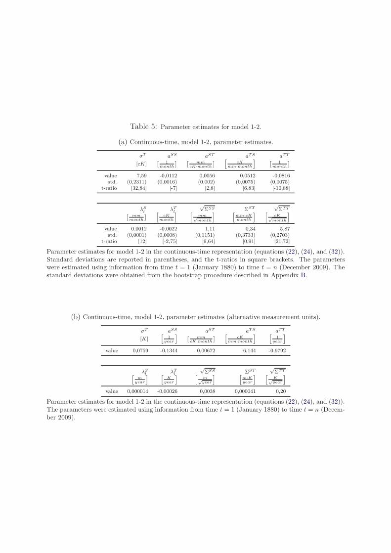
Table 5: Parameter estimates for model 1-2.

(a) Continuous-time, model 1-2, parameter estimates.

σT aSS aST aTS aTT

[cK][

1

month

] [

mmcK·month

]

[

cKmm·month

]

[

1

month

]

value 7,59 -0,0112 0,0056 0,0512 -0,0816std. (0,2311) (0,0016) (0,002) (0,0075) (0,0075)

t-ratio [32,84] [-7] [2,8] [6,83] [-10,88]

λSl

λTl

√ΣSS ΣST

√ΣTT

[

mmmonth

]

[

cKmonth

] [

mm√month

] [

mm·cKmonth

] [

cK√month

]

value 0,0012 -0,0022 1,11 0,34 5,87std. (0,0001) (0,0008) (0,1151) (0,3733) (0,2703)

t-ratio [12] [-2,75] [9,64] [0,91] [21,72]

Parameter estimates for model 1-2 in the continuous-time representation (equations (22), (24), and (32)).Standard deviations are reported in parentheses, and the t-ratios in square brackets. The parameterswere estimated using information from time t = 1 (January 1880) to time t = n (December 2009). Thestandard deviations were obtained from the bootstrap procedure described in Appendix B.

(b) Continuous-time, model 1-2, parameter estimates (alternative measurement units).

σT aSS aST aTS aTT

[K][

1

year

]

[

mmcK·month

]

[

cKmm·month

] [

1

year

]

value 0,0759 -0,1344 0,00672 6,144 -0,9792

λSl

λTl

√ΣSS ΣST

√ΣTT

[

myear

] [

Kyear

] [

m√year

] [

m·Kyear

] [

K√year

]

value 0,000014 -0,00026 0,0038 0,000041 0,20

Parameter estimates for model 1-2 in the continuous-time representation (equations (22), (24), and (32)).The parameters were estimated using information from time t = 1 (January 1880) to time t = n (Decem-ber 2009).

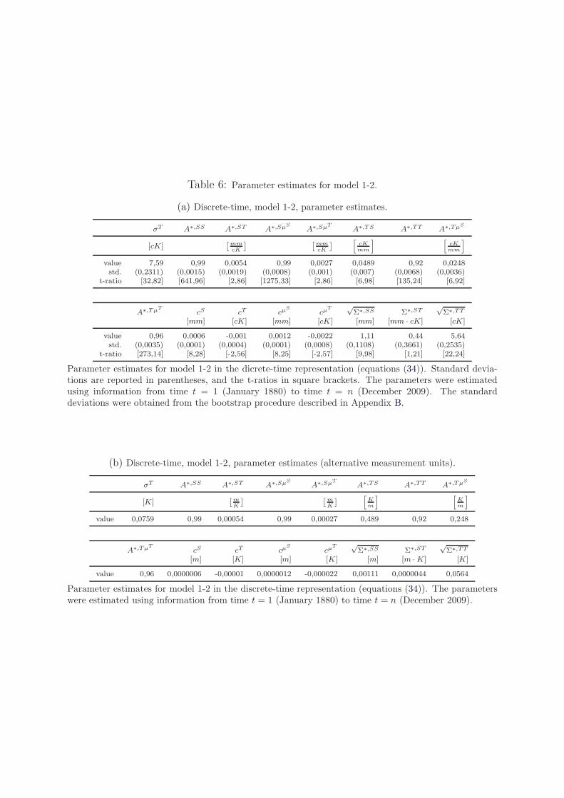
Table 6: Parameter estimates for model 1-2.

(a) Discrete-time, model 1-2, parameter estimates.

σT A∗,SS A∗,ST A∗,SµS

A∗,SµT

A∗,TS A∗,TT A∗,TµS

[cK][

mmcK

] [

mmcK

]

[

cKmm

] [

cKmm

]

value 7,59 0,99 0,0054 0,99 0,0027 0,0489 0,92 0,0248std. (0,2311) (0,0015) (0,0019) (0,0008) (0,001) (0,007) (0,0068) (0,0036)

t-ratio [32,82] [641,96] [2,86] [1275,33] [2,86] [6,98] [135,24] [6,92]

A∗,TµT

cS cT cµS

cµT

√Σ∗,SS Σ∗,ST

√Σ∗,TT

[mm] [cK] [mm] [cK] [mm] [mm · cK] [cK]

value 0,96 0,0006 -0,001 0,0012 -0,0022 1,11 0,44 5,64std. (0,0035) (0,0001) (0,0004) (0,0001) (0,0008) (0,1108) (0,3661) (0,2535)

t-ratio [273,14] [8,28] [-2,56] [8,25] [-2,57] [9,98] [1,21] [22,24]

Parameter estimates for model 1-2 in the dicrete-time representation (equations (34)). Standard devia-tions are reported in parentheses, and the t-ratios in square brackets. The parameters were estimatedusing information from time t = 1 (January 1880) to time t = n (December 2009). The standarddeviations were obtained from the bootstrap procedure described in Appendix B.

(b) Discrete-time, model 1-2, parameter estimates (alternative measurement units).

σT A∗,SS A∗,ST A∗,SµS

A∗,SµT

A∗,TS A∗,TT A∗,TµS

[K][

mK

] [

mK

]

[

Km

] [

Km

]

value 0,0759 0,99 0,00054 0,99 0,00027 0,489 0,92 0,248

A∗,TµT

cS cT cµS

cµT √

Σ∗,SS Σ∗,ST√Σ∗,TT

[m] [K] [m] [K] [m] [m ·K] [K]

value 0,96 0,0000006 -0,00001 0,0000012 -0,000022 0,00111 0,0000044 0,0564

Parameter estimates for model 1-2 in the discrete-time representation (equations (34)). The parameterswere estimated using information from time t = 1 (January 1880) to time t = n (December 2009).

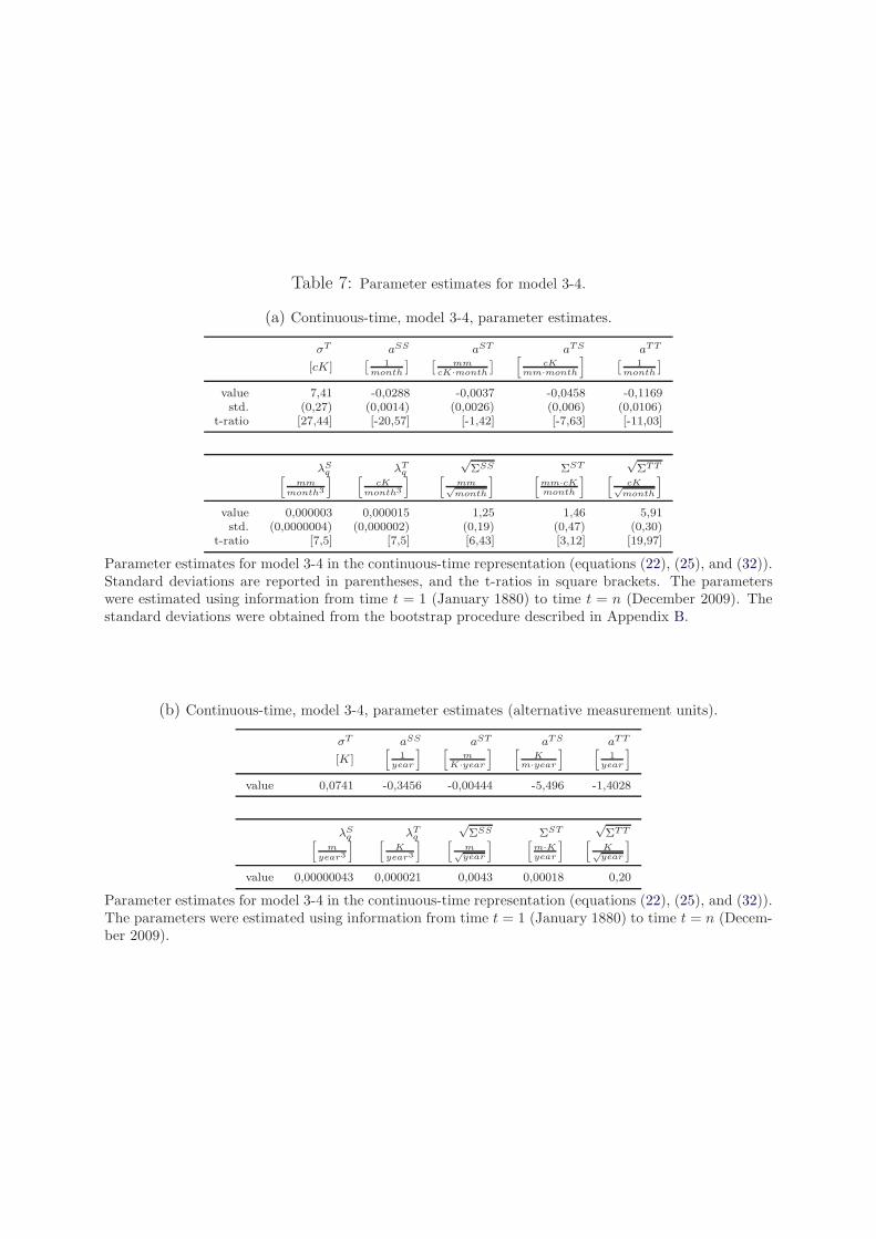
Table 7: Parameter estimates for model 3-4.

(a) Continuous-time, model 3-4, parameter estimates.

σT aSS aST aTS aTT

[cK][

1

month

] [

mmcK·month

]

[

cKmm·month

]

[

1

month

]

value 7,41 -0,0288 -0,0037 -0,0458 -0,1169std. (0,27) (0,0014) (0,0026) (0,006) (0,0106)

t-ratio [27,44] [-20,57] [-1,42] [-7,63] [-11,03]

λSq λT

q

√ΣSS ΣST

√ΣTT

[

mmmonth3

] [

cKmonth3

] [

mm√month

] [

mm·cKmonth

] [

cK√month

]

value 0,000003 0,000015 1,25 1,46 5,91std. (0,0000004) (0,000002) (0,19) (0,47) (0,30)

t-ratio [7,5] [7,5] [6,43] [3,12] [19,97]

Parameter estimates for model 3-4 in the continuous-time representation (equations (22), (25), and (32)).Standard deviations are reported in parentheses, and the t-ratios in square brackets. The parameterswere estimated using information from time t = 1 (January 1880) to time t = n (December 2009). Thestandard deviations were obtained from the bootstrap procedure described in Appendix B.

(b) Continuous-time, model 3-4, parameter estimates (alternative measurement units).

σT aSS aST aTS aTT

[K][

1

year

] [

mK·year

] [

Km·year

] [

1

year

]

value 0,0741 -0,3456 -0,00444 -5,496 -1,4028

λSq λT

q

√ΣSS ΣST

√ΣTT

[

myear3

] [

Kyear3

] [

m√year

] [

m·Kyear

] [

K√year

]

value 0,00000043 0,000021 0,0043 0,00018 0,20

Parameter estimates for model 3-4 in the continuous-time representation (equations (22), (25), and (32)).The parameters were estimated using information from time t = 1 (January 1880) to time t = n (Decem-ber 2009).

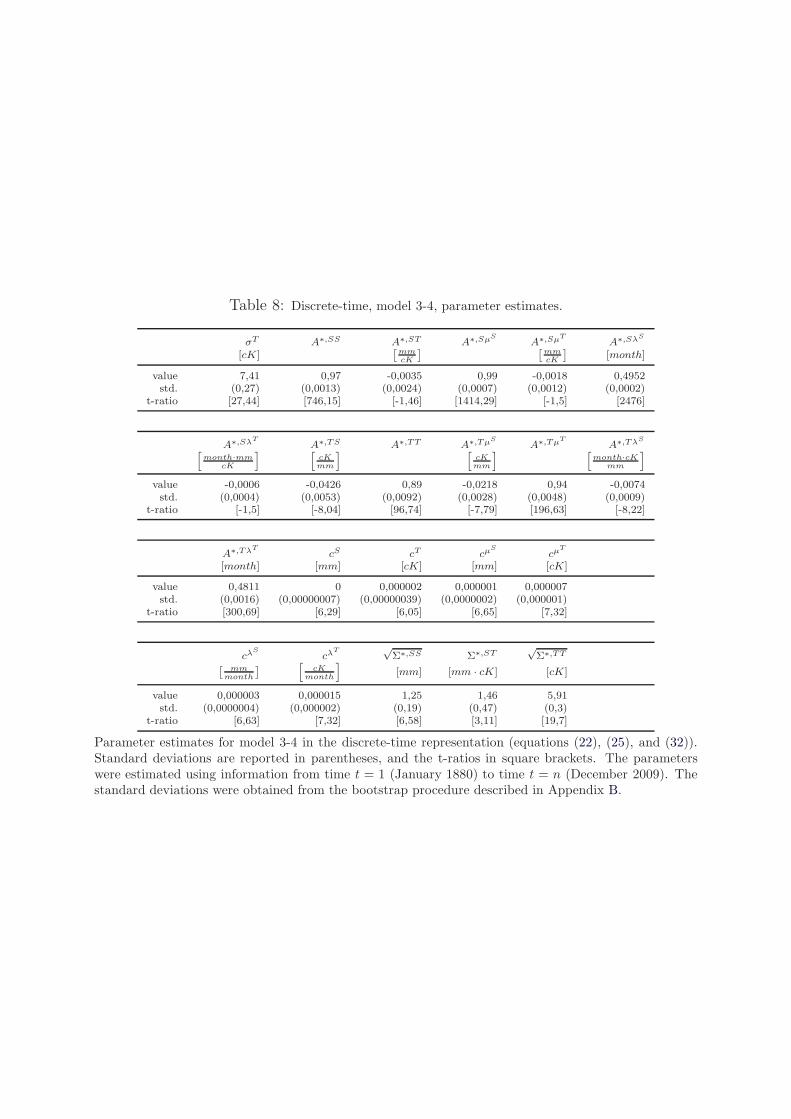
Table 8: Discrete-time, model 3-4, parameter estimates.

σT A∗,SS A∗,ST A∗,SµS

A∗,SµT

A∗,SλS

[cK][

mmcK

] [

mmcK

]

[month]

value 7,41 0,97 -0,0035 0,99 -0,0018 0,4952std. (0,27) (0,0013) (0,0024) (0,0007) (0,0012) (0,0002)

t-ratio [27,44] [746,15] [-1,46] [1414,29] [-1,5] [2476]

A∗,SλT

A∗,TS A∗,TT A∗,TµS

A∗,TµT

A∗,TλS

[

month·mmcK

] [

cKmm

] [

cKmm

] [

month·cKmm

]

value -0,0006 -0,0426 0,89 -0,0218 0,94 -0,0074std. (0,0004) (0,0053) (0,0092) (0,0028) (0,0048) (0,0009)

t-ratio [-1,5] [-8,04] [96,74] [-7,79] [196,63] [-8,22]

A∗,TλT

cS cT cµS

cµT

[month] [mm] [cK] [mm] [cK]

value 0,4811 0 0,000002 0,000001 0,000007std. (0,0016) (0,00000007) (0,00000039) (0,0000002) (0,000001)

t-ratio [300,69] [6,29] [6,05] [6,65] [7,32]

cλS

cλT

√Σ∗,SS Σ∗,ST

√Σ∗,TT

[

mmmonth

]

[

cKmonth

]

[mm] [mm · cK] [cK]

value 0,000003 0,000015 1,25 1,46 5,91std. (0,0000004) (0,000002) (0,19) (0,47) (0,3)

t-ratio [6,63] [7,32] [6,58] [3,11] [19,7]

Parameter estimates for model 3-4 in the discrete-time representation (equations (22), (25), and (32)).Standard deviations are reported in parentheses, and the t-ratios in square brackets. The parameterswere estimated using information from time t = 1 (January 1880) to time t = n (December 2009). Thestandard deviations were obtained from the bootstrap procedure described in Appendix B.

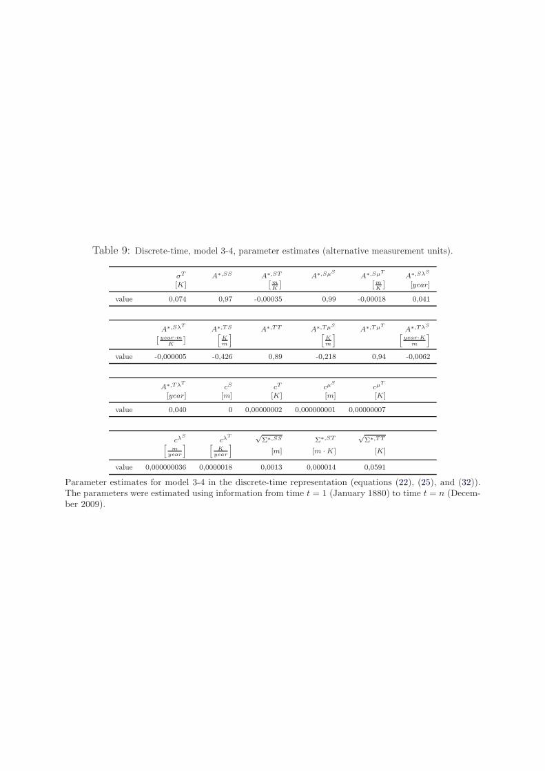
Table 9: Discrete-time, model 3-4, parameter estimates (alternative measurement units).

σT A∗,SS A∗,ST A∗,SµS

A∗,SµT

A∗,SλS

[K][

mK

] [

mK

]

[year]

value 0,074 0,97 -0,00035 0,99 -0,00018 0,041

A∗,SλT

A∗,TS A∗,TT A∗,TµS

A∗,TµT

A∗,TλS

[

year·mK

]

[

Km

] [

Km

] [

year·Km

]

value -0,000005 -0,426 0,89 -0,218 0,94 -0,0062

A∗,TλT

cS cT cµS

cµT

[year] [m] [K] [m] [K]

value 0,040 0 0,00000002 0,000000001 0,00000007

cλS

cλT

√Σ∗,SS Σ∗,ST

√Σ∗,TT

[

myear

] [

Kyear

]

[m] [m ·K] [K]

value 0,000000036 0,0000018 0,0013 0,000014 0,0591

Parameter estimates for model 3-4 in the discrete-time representation (equations (22), (25), and (32)).The parameters were estimated using information from time t = 1 (January 1880) to time t = n (Decem-ber 2009).

Research Papers 2013

2015-23: Eric Hillebrand, Søren Johansen and Torben Schmith: Data revisions and the statistical relation of global mean sea-level and temperature

2015-24: Tommaso Proietti and Alessandra Luati: Generalised partial autocorrelations and the mutual information between past and future

2015-25: Bent Jesper Christensen and Rasmus T. Varneskov: Medium Band Least Squares Estimation of Fractional Cointegration in the Presence of Low-Frequency Contamination

2015-26: Ulrich Hounyo and Rasmus T. Varneskov: A Local Stable Bootstrap for Power Variations of Pure-Jump Semimartingales and Activity Index Estimation

2015-27: Rasmus Søndergaard Pedersen and Anders Rahbek: Nonstationary ARCH and GARCH with t-distributed Innovations

2015-28: Tommaso Proietti and Eric Hillebrand: Seasonal Changes in Central England Temperatures

2015-29: Laurent Callot and Johannes Tang Kristensen: Regularized Estimation of Structural Instability in Factor Models: The US Macroeconomy and the Great Moderation

2015-30: Davide Delle Monache, Stefano Grassi and Paolo Santucci de Magistris: Testing for Level Shifts in Fractionally Integrated Processes: a State Space Approach

2015-31: Matias D. Cattaneo, Michael Jansson and Whitney K. Newey: Treatment Effects with Many Covariates and Heteroskedasticity

2015-32: Jean-Guy Simonato and Lars Stentoft: Which pricing approach for options under GARCH with non-normal innovations?

2015-33: Nina Munkholt Jakobsen and Michael Sørensen: Efficient Estimation for Diffusions Sampled at High Frequency Over a Fixed Time Interval

2015-34: Wei Wei and Denis Pelletier: A Jump-Diffusion Model with Stochastic Volatility and Durations

2015-35: Yunus Emre Ergemen and Carlos Velasco: Estimation of Fractionally Integrated Panels with Fixed Effects and Cross-Section Dependence

2015-36: Markku Lanne and Henri Nyberg: Nonlinear dynamic interrelationships between real activity and stock returns

2015-37: Markku Lanne and Jani Luoto: Estimation of DSGE Models under Diffuse Priors and Data-Driven Identification Constraints

2015-38: Lorenzo Boldrini and Eric Hillebrand: Supervision in Factor Models Using a Large Number of Predictors

2015-39: Lorenzo Boldrini and Eric Hillebrand: The Forecasting Power of the Yield Curve, a Supervised Factor Model Approach

2015-40: Lorenzo Boldrini: Forecasting the Global Mean Sea Level, a Continuous-Time State-Space Approach