Embed Size (px)
Citation preview
Forecasting Seasonal Time Series∗
Philip Hans FransesEconometric Institute, Erasmus University Rotterdam
September 6, 2004
Abstract
This chapter deals with seasonal time series in economics and it reviewsmodels that can be used to forecast out-of-sample data. Some of the key prop-erties of seasonal time series are reviewed, and various empirical examples aregiven for illustration. The potential limitations to seasonal adjustment arereviewed. The chapter further addresses a few basic models like the deter-ministic seasonality model and the airline model, and it shows what featuresof the data these models assume to have. Then, the chapter continues withmore advanced models, like those concerning seasonal and periodic unit roots.Finally, there is a discussion of some recent advances, which mainly concernmodels which allow for links between seasonal variation and heteroskedasticityand non-linearity.
Key words and phrases: Forecasting, seasonality, unit roots, periodic models,cointegration
∗Work on this chapter started when the author was enjoying the hospitality of the Institute ofMathematical Statistics, National University of Singapore (April 2004). Thanks are due to Dickvan Dijk and Marnik Dekimpe for their help with the data. All computations have been made usingEviews (version 4.1). Details of estimation results not reported in this chapter can be obtainedfrom the author. A full list of relevant references is also available. The address for correspondenceis Econometric Institute, Erasmus University Rotterdam, P.O. Box 1738, NL-3000 DR Rotterdam,email: [email protected]
1

Contents
1 Introduction 1
2 Seasonal time series 2
3 Basic Models 15
4 Advanced Models 24
5 Recent advances 33
6 Conclusion 36
0
1 Introduction
This chapter deals with seasonal time series in economics and it reviews models
that can be used to forecast out-of-sample data. A seasonal time series is assumed
to be a series measured at a frequency t where this series shows certain recurrent
patterns within a frequency T , with t = ST . For example, quarterly data (t) can
show different means and variances within a year (4T ). Similar phenomena can
appear for hourly data within days, daily data within weeks, monthly data within
years, and so on. Examples of data with pronounced recurrent patterns are quarterly
nondurable consumption, monthly industrial production, daily retail sales (within
a week), hourly referrals after broadcasting a TV commercial (within a day), and
stock price changes measured per minute within a day.
A trend is important to extrapolate accurately when forecasting longer horizons
ahead. Seasonality is important to properly take care off when forecasting the next
S or kS out-of-sample data, with k not very large, hence the medium term. This
chapter reviews models that can be usefully implemented for that purpose. The
technical detail is kept at a moderate level, and extensive reference will be made
to the studies which contain all the details. Important books in this context are
Hylleberg (1992), Ghysels and Osborn (2001), and Franses and Paap (2004). The
recent survey of Brendstrup et al. (2004) is excellent, also as it contains a useful
and rather exhaustive list of references.
The outline of this chapter is a follows. In Section 2, I discuss some of the key
properties of seasonal time series. I use a few empirical examples for illustration.
Next, I discuss the potential limitations to seasonal adjustment. In Section 3, I
review basic models like the deterministic seasonality model and the airline model,
and show features of the data these models assume they have. In Section 4, I continue
with more advanced models, like those concerning seasonal and periodic unit roots.
Section 5 deals with some recent advances, which mainly concern models which
allow for links between seasonal variation and heteroskedasticity and non-linearity.
Section 6 concludes with a summary of important future research areas.
1
2 Seasonal time series
This section deals with various features of seasonally observed time series that one
might want to capture in an econometric time series model. Next, the discussion
focuses on what it is that one intends to forecast. Finally, I address the issue why
seasonal adjustment often is problematic.
How do seasonal time series look like?
In this chapter I use a few series for illustration. The typical tools to see how sea-
sonal variation in a series might look like, and hence which time series models might
be considered to start with, are (i) graphs (over time, or per season), (ii) auto-
correlations (usually after somehow removing the trend, where it is not uncommon
to use the first differencing filter ∆1yt = yt − yt−1), (iii) the R2 of a regression of
∆1yt on S seasonal dummies or on S (or less) sines and cosines, (iv) a regression
of squared residuals from a time series model for ∆1yt on an intercept and S − 1
seasonal dummies (to check for seasonal variation in error variance), and finally (v)
autocorrelations per season (to see if there is periodicity). With periodicity one typ-
ically means that correlations within or across variables can change with the season,
see Franses and Paap (2004) for an up to date survey. It should noted that these are
all just first-stage tools, to see in which direction one could proceed. They should
not be interpreted as final models or methods, as they usually do not fully capture
all relevant aspects of the time series.
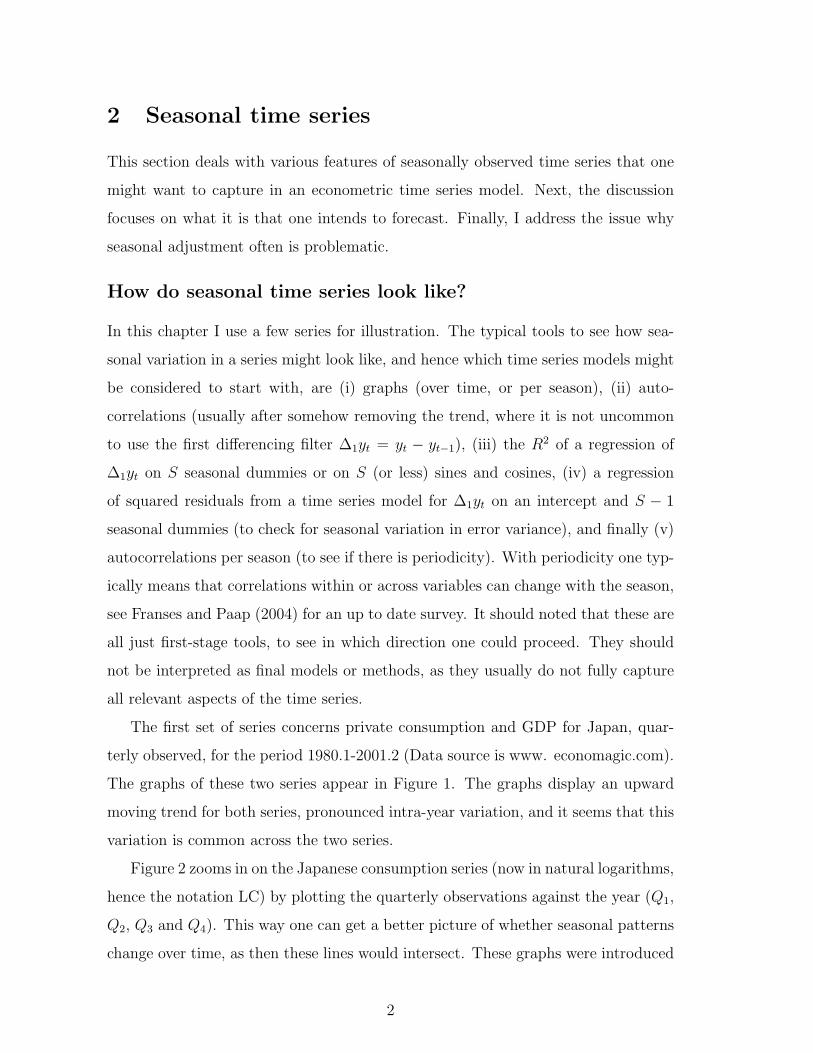
The first set of series concerns private consumption and GDP for Japan, quar-
terly observed, for the period 1980.1-2001.2 (Data source is www. economagic.com).
The graphs of these two series appear in Figure 1. The graphs display an upward
moving trend for both series, pronounced intra-year variation, and it seems that this
variation is common across the two series.
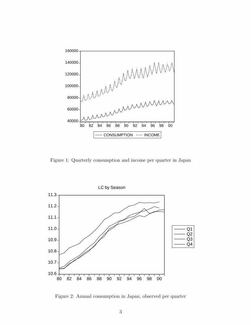
Figure 2 zooms in on the Japanese consumption series (now in natural logarithms,
hence the notation LC) by plotting the quarterly observations against the year (Q1,
Q2, Q3 and Q4). This way one can get a better picture of whether seasonal patterns
change over time, as then these lines would intersect. These graphs were introduced
2
40000
60000
80000
100000
120000
140000
160000
80 82 84 86 88 90 92 94 96 98 00
CONSUMPTION INCOME
Figure 1: Quarterly consumption and income per quarter in Japan
10.6
10.7
10.8
10.9
11.0
11.1
11.2
11.3
80 82 84 86 88 90 92 94 96 98 00
Q1Q2Q3Q4
LC by Season
Figure 2: Annual consumption in Japan, observed per quarter
3
in Franses (1991, 1994) and now appear in Eviews (version 4.1) as ”split seasonals”.
For the Japanese consumption series one can observe that there is a slight change
in seasonality towards the end of the sample, but mostly the seasonal pattern seems
rather stable over time.
For these two series, after taking natural logs, the R2 of the ”seasonal dummy
regression” for ∆1yt, that is,
∆1yt =4∑
s=1
δsDs,t + εt, (1)
is 0.927 for log(consumption) and for log(income) it is 0.943. The Ds,t variables
obtain a value 1 in seasons s and a 0 elsewhere. Note that it is unlikely that εt
matches with a white noise time series, but then still, the values of these R2 measures
are high. Franses, Hylleberg and Lee (1995) show that the size of this R2 can be
misinterpreted in case of neglected unit roots, but for the moment this regression is
informative.
A suitable first-attempt model for both Japanese log(consumption) and log(income)
is
∆1yt =4∑
s=1
δsDs,t + ρ1∆1yt−1 + εt + θ4εt−4. (2)
where ρ1 is estimated to be -0.559 (0.094) and -0.525 (0.098), respectively (with
standard errors in parentheses), and where θ4 is estimated to be 0.441 (0.100) and
0.593 (0.906), respectively. Relative to (1), the R2 of these models have increased
to 0.963 and 0.975, respectively, suggesting that constant deterministic seasonality
seems to account for the majority of trend-free variation in the data.
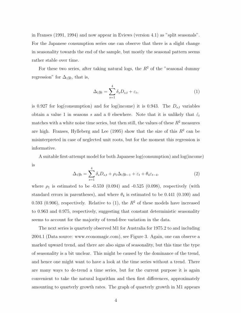
The next series is quarterly observed M1 for Australia for 1975.2 to and including
2004.1 (Data source: www.economagic.com), see Figure 3. Again, one can observe a
marked upward trend, and there are also signs of seasonality, but this time the type
of seasonality is a bit unclear. This might be caused by the dominance of the trend,
and hence one might want to have a look at the time series without a trend. There
are many ways to de-trend a time series, but for the current purpose it is again
convenient to take the natural logarithm and then first differences, approximately
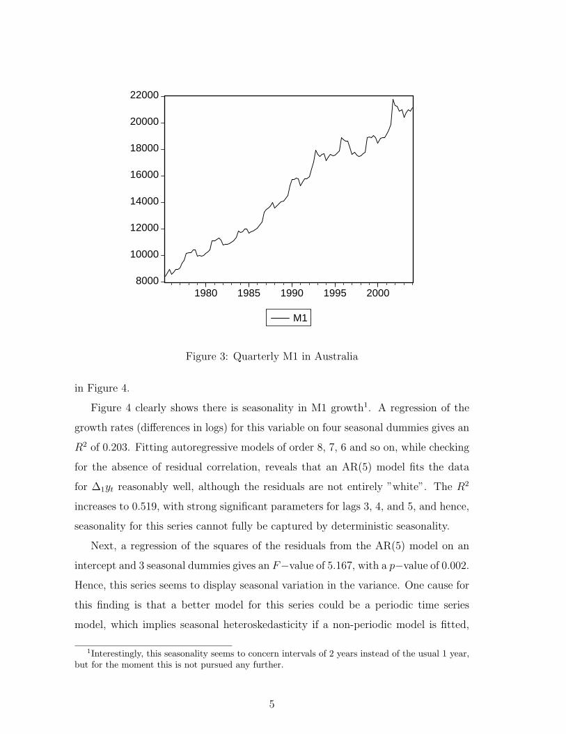
amounting to quarterly growth rates. The graph of quarterly growth in M1 appears
4
8000
10000
12000
14000
16000
18000
20000
22000
1980 1985 1990 1995 2000
M1
Figure 3: Quarterly M1 in Australia
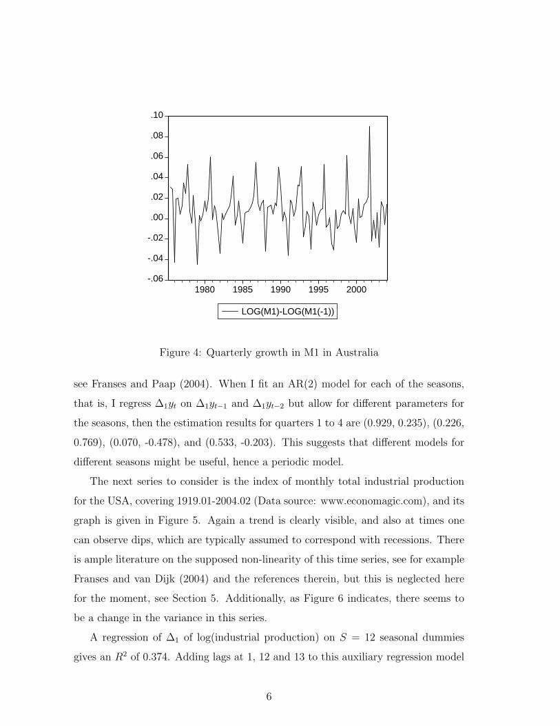
in Figure 4.
Figure 4 clearly shows there is seasonality in M1 growth1. A regression of the
growth rates (differences in logs) for this variable on four seasonal dummies gives an
R2 of 0.203. Fitting autoregressive models of order 8, 7, 6 and so on, while checking
for the absence of residual correlation, reveals that an AR(5) model fits the data
for ∆1yt reasonably well, although the residuals are not entirely ”white”. The R2
increases to 0.519, with strong significant parameters for lags 3, 4, and 5, and hence,
seasonality for this series cannot fully be captured by deterministic seasonality.
Next, a regression of the squares of the residuals from the AR(5) model on an
intercept and 3 seasonal dummies gives an F−value of 5.167, with a p−value of 0.002.
Hence, this series seems to display seasonal variation in the variance. One cause for
this finding is that a better model for this series could be a periodic time series
model, which implies seasonal heteroskedasticity if a non-periodic model is fitted,
1Interestingly, this seasonality seems to concern intervals of 2 years instead of the usual 1 year,but for the moment this is not pursued any further.
5
-.06
-.04
-.02
.00
.02
.04
.06
.08
.10
1980 1985 1990 1995 2000
LOG(M1)-LOG(M1(-1))
Figure 4: Quarterly growth in M1 in Australia
see Franses and Paap (2004). When I fit an AR(2) model for each of the seasons,
that is, I regress ∆1yt on ∆1yt−1 and ∆1yt−2 but allow for different parameters for
the seasons, then the estimation results for quarters 1 to 4 are (0.929, 0.235), (0.226,
0.769), (0.070, -0.478), and (0.533, -0.203). This suggests that different models for
different seasons might be useful, hence a periodic model.
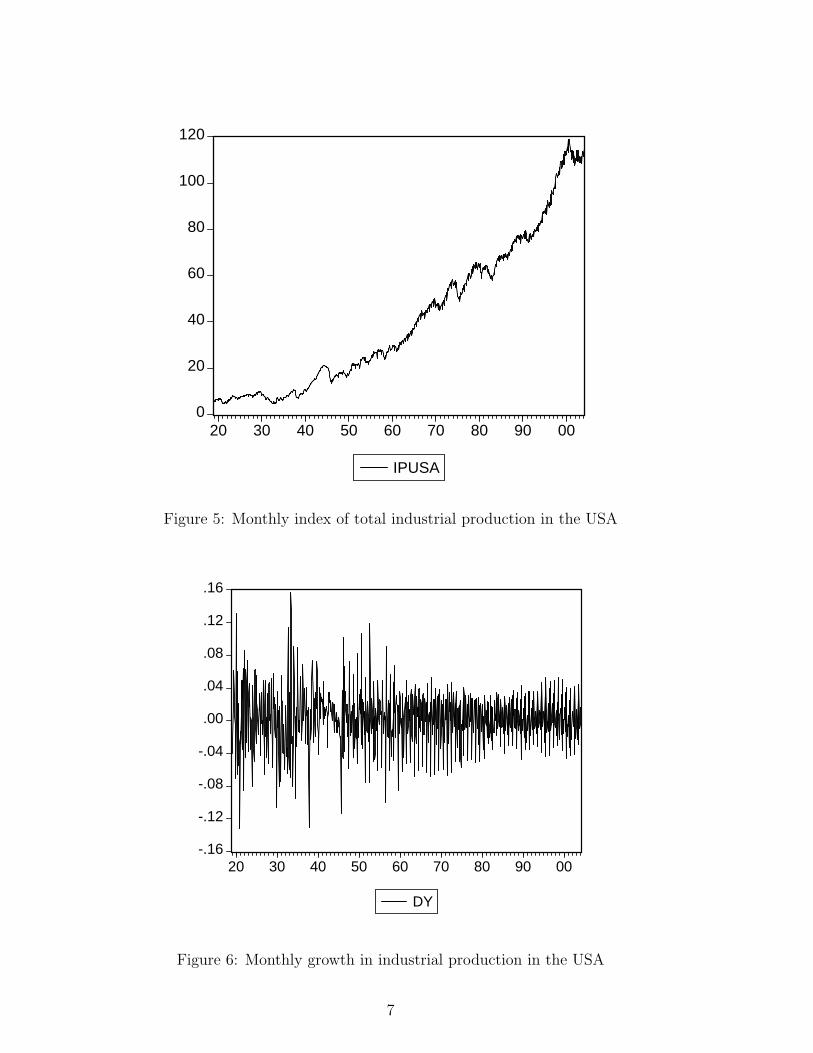
The next series to consider is the index of monthly total industrial production
for the USA, covering 1919.01-2004.02 (Data source: www.economagic.com), and its
graph is given in Figure 5. Again a trend is clearly visible, and also at times one
can observe dips, which are typically assumed to correspond with recessions. There
is ample literature on the supposed non-linearity of this time series, see for example
Franses and van Dijk (2004) and the references therein, but this is neglected here
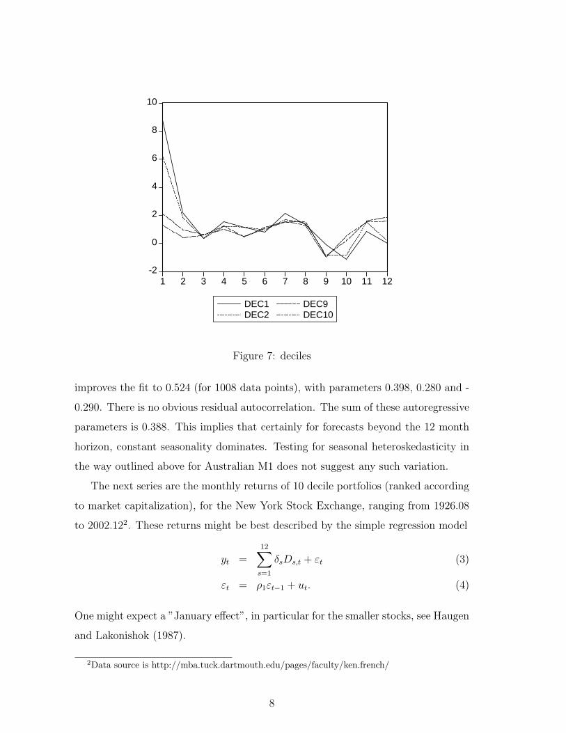
for the moment, see Section 5. Additionally, as Figure 6 indicates, there seems to
be a change in the variance in this series.
A regression of ∆1 of log(industrial production) on S = 12 seasonal dummies
gives an R2 of 0.374. Adding lags at 1, 12 and 13 to this auxiliary regression model
6
0
20
40
60
80
100
120
20 30 40 50 60 70 80 90 00
IPUSA
Figure 5: Monthly index of total industrial production in the USA
-.16
-.12
-.08
-.04
.00
.04
.08
.12
.16
20 30 40 50 60 70 80 90 00
DY
Figure 6: Monthly growth in industrial production in the USA
7
-2
0
2
4
6
8
10
1 2 3 4 5 6 7 8 9 10 11 12
DEC1DEC2
DEC9DEC10
Figure 7: deciles
improves the fit to 0.524 (for 1008 data points), with parameters 0.398, 0.280 and -
0.290. There is no obvious residual autocorrelation. The sum of these autoregressive
parameters is 0.388. This implies that certainly for forecasts beyond the 12 month
horizon, constant seasonality dominates. Testing for seasonal heteroskedasticity in
the way outlined above for Australian M1 does not suggest any such variation.
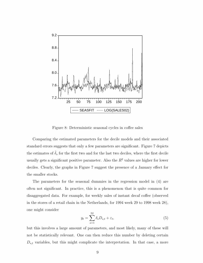
The next series are the monthly returns of 10 decile portfolios (ranked according
to market capitalization), for the New York Stock Exchange, ranging from 1926.08
to 2002.122. These returns might be best described by the simple regression model
yt =12∑
s=1
δsDs,t + εt (3)
εt = ρ1εt−1 + ut. (4)
One might expect a ”January effect”, in particular for the smaller stocks, see Haugen
and Lakonishok (1987).
2Data source is http://mba.tuck.dartmouth.edu/pages/faculty/ken.french/
8
7.2
7.6
8.0
8.4
8.8
9.2
25 50 75 100 125 150 175 200
SEASFIT LOG(SALES02)
Figure 8: Deterministic seasonal cycles in coffee sales
Comparing the estimated parameters for the decile models and their associated
standard errors suggests that only a few parameters are significant. Figure 7 depicts
the estimates of δs for the first two and for the last two deciles, where the first decile
usually gets a significant positive parameter. Also the R2 values are higher for lower
deciles. Clearly, the graphs in Figure 7 suggest the presence of a January effect for
the smaller stocks.
The parameters for the seasonal dummies in the regression model in (4) are
often not significant. In practice, this is a phenomenon that is quite common for
disaggregated data. For example, for weekly sales of instant decaf coffee (observed
in the stores of a retail chain in the Netherlands, for 1994 week 29 to 1998 week 28),
one might consider
yt =52∑
s=1
δsDs,t + εt, (5)
but this involves a large amount of parameters, and most likely, many of these will
not be statistically relevant. One can then reduce this number by deleting certain
Ds,t variables, but this might complicate the interpretation. In that case, a more
9
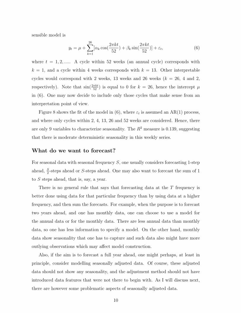
sensible model is
yt = µ +26∑
k=1
[αk cos(2πkt
52) + βk sin(
2πkt
52)] + εt, (6)
where t = 1, 2, ..... A cycle within 52 weeks (an annual cycle) corresponds with
k = 1, and a cycle within 4 weeks corresponds with k = 13. Other interpretable
cycles would correspond with 2 weeks, 13 weeks and 26 weeks (k = 26, 4 and 2,
respectively). Note that sin(2πkt52
) is equal to 0 for k = 26, hence the intercept µ
in (6). One may now decide to include only those cycles that make sense from an
interpretation point of view.
Figure 8 shows the fit of the model in (6), where εt is assumed an AR(1) process,
and where only cycles within 2, 4, 13, 26 and 52 weeks are considered. Hence, there
are only 9 variables to characterize seasonality. The R2 measure is 0.139, suggesting
that there is moderate deterministic seasonality in this weekly series.
What do we want to forecast?
For seasonal data with seasonal frequency S, one usually considers forecasting 1-step
ahead, S2-steps ahead or S-steps ahead. One may also want to forecast the sum of 1
to S steps ahead, that is, say, a year.
There is no general rule that says that forecasting data at the T frequency is
better done using data for that particular frequency than by using data at a higher
frequency, and then sum the forecasts. For example, when the purpose is to forecast
two years ahead, and one has monthly data, one can choose to use a model for
the annual data or for the monthly data. There are less annual data than monthly
data, so one has less information to specify a model. On the other hand, monthly
data show seasonality that one has to capture and such data also might have more
outlying observations which may affect model construction.
Also, if the aim is to forecast a full year ahead, one might perhaps, at least in
principle, consider modelling seasonally adjusted data. Of course, these adjusted
data should not show any seasonality, and the adjustment method should not have
introduced data features that were not there to begin with. As I will discuss next,
there are however some problematic aspects of seasonally adjusted data.
10

Why is seasonal adjustment often problematic?
It is common practice to seasonally adjust quarterly or monthly observed macro-
economic time series, like GDP and unemployment. A key motivation is that prac-
titioners seem to want to compare the current observation with that in the previous
month or quarter, without considering seasonality. As many series display seasonal
fluctuations which are not constant over time, at least not for the typical time span
considered in practice, there is a debate in the statistics and econometrics litera-
ture about which method is most useful for seasonal adjustment. Roughly speaking,
there are two important methods. The first is the Census X-11 method, initiated by
Shiskin and Eisenpress (1957), and the second one uses model-based methods, see
for example Maravall (1995). Interestingly, it seems that with the new Census X-12
method, the two approaches have come closer together, see Findley et al. (1998). In
Franses (2001) I address the question why one would want to seasonally adjust in
the first place, and what follows in this subsection draws upon that discussion.
Except for macroeconomics, there is no economic discipline in which the data are
seasonally adjusted prior to analysis. It is hard to imagine, for example, that there
would be a stock market index, with returns corrected for day-of-the-week effects.
Also, seasonality in sales or market shares is of particular interest to a manager, and
seasonal adjustment of marketing data would simply result in an uninteresting time
series.
Generally, the interest in analyzing macroeconomic data concerns the trend and
the business cycle. In case the data have stochastic trends, one usually resorts to
well-known techniques for common trends analysis and cointegration, see for example
Engle and Granger (1991). To understand business cycle fluctuations, for example
in the sense of examining which variables seem to be able to predict recessions,
one can use nonlinear models like the (smooth transition) threshold model and the
Markov-switching model, see Granger and Terasvirta (1993) and Franses and van
Dijk (2000) for surveys.
Consider a seasonally observed time series yt, where t runs from 1 to n. In
practice one might be interested in the seasonally adjusted observation at time n or
11
n − 1. The main purpose of seasonal adjustment is to separate the observed data
into two components, a nonseasonal component and a seasonal component. These
components are not observed, and have to be estimated from the data. It is assumed
that
yt = yNSt + yS
t , (7)
where yNSt is the estimated nonseasonal component, and yS
t is the estimated seasonal
component. This decomposition assumes an additive relation. When this is not the
case, one can transform yt until it holds for the transformed data. For example, if
the seasonal fluctuations seem multiplicative with the trend, one typically considers
the natural logarithmic transformation.
As said, there are two commonly used approaches to estimate the components in
(7). The first is coined Census X-12. This approach applies a sequence of two-sided
moving average filters like
w0 +m∑
i=1
wi(Li + L−i), (8)
where L is the familiar backward shift operator, and where the value of m and the
weights wi for i = 0, 1, . . . , m are set by the practitioner. It additionally contains
a range of outlier removal methods, and corrections for trading-day and holiday
effects. An important consequence of two-sided filters is that to adjust observation
yn, one needs the observations at time n + 1, n + 2 to n + m. As these are not
yet observed at n, one has to rely on forecasted values, which are then treated as
genuine observations. Of course, this automatically implies that seasonally adjusted
data should be revised after a while, especially if the newly observed realizations
differ from those forecasts. Interesting surveys of this method are given in Bell and
Hillmer (1984), Hylleberg (1986), and more recently in Findley et al. (1998).
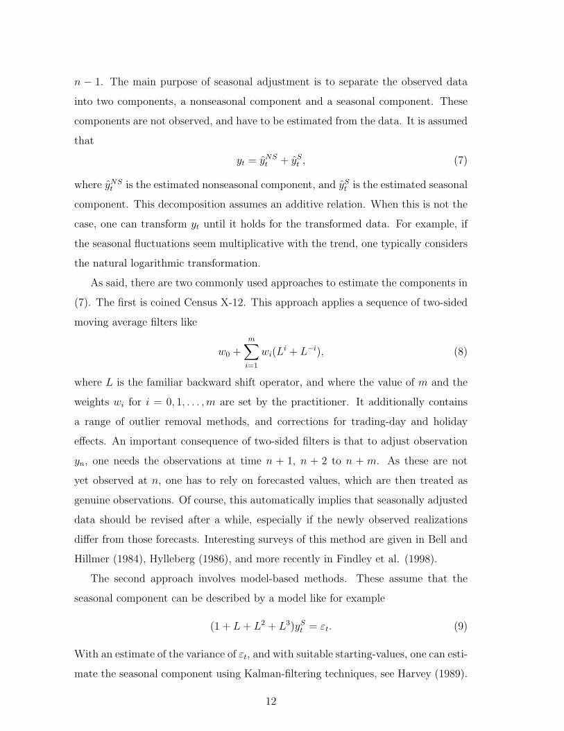
The second approach involves model-based methods. These assume that the
seasonal component can be described by a model like for example
(1 + L + L2 + L3)ySt = εt. (9)
With an estimate of the variance of εt, and with suitable starting-values, one can esti-
mate the seasonal component using Kalman-filtering techniques, see Harvey (1989).
12
Given ySt , one can simply use (7) to get the estimated adjusted series.
A few remarks can be made. The first amounts to recognizing that seasonally ad-
justed data are estimated data. In practice this might be forgotten, which is mainly
due to the fact that those who provide the seasonally adjusted data tend not to pro-
vide the associated standard errors. This is misleading. Indeed, a correct statement
would read ”this month’s unemployment rate is 7.8, and after seasonal adjustment it
is 7.5 plus or minus 0.3”. The Census X-12 method cannot generate standard errors,
but for the model-based methods it is not difficult to do so. Koopman and Franses
(2003) propose a method which also allows for business cylce-dependent confidence
intervals around seasonally adjusted data.
Obviously, when yNSt is saved and yS
t is thrown away, one cannot reconstruct
the original series yt. Moreover, if the original series yt can be described by an
econometric time series model with innovations εt, it is unclear to what extent these
innovations are assigned to either yNSt , yS
t or to both. Hence, when one constructs an
econometric time series model for the adjusted series yNSt , the estimated innovations
in this model are not the ”true” innovations. This feature makes impulse-response
analysis less interesting.
The key assumption is the relation in (7). For some economic time series this
relation does not hold. For example, if the data can best be described by a so-called
periodic time series model, where the parameters vary with the seasons, see Section
4 below, one cannot separate out a seasonal component and reliably focus on the
estimated nonseasonal component. There are a few theoretical results about what
exactly happens if one adjusts a periodic series, and some simulation and empirical
results are available, see Franses (1996), Ooms and Franses (1997) and Del Barrio
Castro and Osborn (2004). Generally, seasonally adjusted periodic data still display
seasonality.
Given the aim of seasonal adjustment, that is, to create time series which are
more easy to analyze for trends and business cycles, it is preferable that seasonally
adjusted data (1) show no signs of seasonality, (2) do not have trend properties
that differ from those of the original data, and (3) that they do not have other
non-linear properties than the original data. Unfortunately, it turns out that most
13
publicly available adjusted data do not have all of these properties. Indeed, it
frequently occurs that yNSt can be modeled using a seasonal ARMA model, with
highly significant parameters at seasonal lags in both the AR and MA parts of
the model. The intuition for this empirical finding may be that two-sided filters
as in (8) can be shown to assume quite a number of so-called seasonal unit roots,
see Section 3 below. Empirical tests for seasonal unit roots in the original series
however usually suggest a smaller number of such roots, and by assuming too many
such roots, seasonal adjustment introduces seasonality in the MA part of the model.
Furthermore, and as mentioned before, if the data correspond with a periodic time
series process, one can still fit a periodic time series model to the adjusted data. The
intuition here is that linear moving average filters treat all observations as equal.
Would seasonal adjustment leave the trend property of the original data intact?
Unfortunately not, as many studies indicate. The general finding is that the per-
sistence of shocks is higher, which in formal test settings usually corresponds with
more evidence in favor of a unit root. In a multivariate framework this amounts to
finding less evidence in favor of cointegration, that is, of the presence of stable long-
run relationships, and thus more evidence of random walk type trends. The possible
intuition of this result is that two-sided filters make the effects of innovations to
appear in 2m + 1 adjusted observations, thereby spuriously creating a higher degree
of persistence of shocks. Hence, seasonal adjustment incurs less evidence of long-run
stability.
Non-linear data do not become linear after seasonal adjustment, but there is
some evidence that otherwise linear data can display non-linearity after seasonal
adjustment, see Ghysels, Granger and Siklos (1996). Additionally, non-linear models
for the original data seem to differ from similar models for the adjusted data. The
structure of the non-linear model does not necessarily change, it merely concerns
the parameters in these models. Hence, one tends to find other dates for recessions
for adjusted data than for unadjusted data. A general finding is that the recessions
for adjusted data last longer. The intuition for this result is that expansion data are
used to adjust recession data and the other way round. Hence, regime switches get
smoothed away or become less pronounced.
14
In sum, seasonally adjusted data may still display some seasonality, can have
different trend properties than the original data have, and also can have different
non-linear properties. It is my opinion that this suggests that these data may not
be useful for their very purpose.
3 Basic Models
This section deals with a few basic models that are often used in practice. They
also often serve as a benchmark, in case one decides to construct more complicated
models. These models are the constant deterministic seasonality model, the seasonal
random walk, the so-called airline model and the basic structural time series model.
The deterministic seasonality model
This first model is useful in case the seasonal pattern is constant over time. This
constancy can be associated with various aspects. First, for some of the data we
tend to analyze in practice, the weather conditions do not change, that is, there is
a intra-year climatological cycle involving precipitation and hours of sunshine that
is rather constant over the years. For example, the harvesting season is reasonably
fixed, it is known when lakes and harbors are ice-free, and our mental status also
seems to experience some fixed seasonality. In fact, consumer survey data (con-
cerning consumer confidence) show seasonality, where such confidence is higher in
January and lower in October, as compared with other months. Some would say
that such seasonality in mood has an impact on stock market fluctuations, and in-
deed, major stock market crashes tend to occur more often in the month of October.
Other regular phenomena concern calender-based festivals and holidays. Finally, in-
stitutional factors as tax years, end-of-years bonuses, and school holidays, can make
some economic phenomena to obey a regular seasonal cycle.
A general model for constant seasonality in case there are S seasons is
yt = µ +
S2∑
k=1
[αk cos(2πkt
S) + βk sin(
2πkt
S)] + ut, (10)
where t = 1, 2, .... and ut is some ARMA type process. This expression makes explicit
15
that constant deterministic seasonality can also be viewed as a sum of cycles, defined
by sines and cosines. For example, for S = 4, one has
yt = µ + α1 cos(1
2πt) + β1 sin(
1
2πt) + α2 cos(πt) + ut, (11)
where cos(12πt) equals (0,-1,0,1,0,-1,...) and sin(1
2πt) is (1,0,-1,0,1,0,...) and cos(πt)
is (-1,1,-1,1,...). The µ is included as sin(πt) is zero everywhere.
The expression in terms of sines and cosines is also relevant as it matches more
naturally with the discussion below on filters. For example, if one considers yt +yt−2
for quarterly data, which can be written as (1 + L2)yt, then (1 + L2) cos(12πt) = 0
and (1 + L2) sin(12πt) = 0. This means that this filter effectively cancels part of the
deterministic seasonal variation. Additionally, it holds that (1+ L) cos(πt) = 0, and
of course, (1−L)µ = 0. This shows that deterministic seasonality can be removed by
applying the transformation (1−L)(1+L)(1+L2) = 1−L4. In words it means that
comparing the current quarter with the same quarter last year effectively removes
the influence of deterministic seasonality, if there would be any, or that of a trends,
again if there would be any. I will return to this transformation later on.
Naturally, there is a one-to-one link between the model in (10) and the model
which has the familiar S seasonal dummy variables. For S = 4, one has
yt =4∑
s=1
δsDs,t + ut, (12)
and it holds that µ =∑4
s=1 δs, and that α1 = δ4 − δ2, β1 = δ1 − δ3 and α2 =
δ4−δ3 +δ2−δ1. There is no particular reason to favor one of the two models, except
for the case where S is large, as I mentioned before. For example, when S is 52, a
model like in (12) contains many parameters, of which many might turn out to be
insignificant in practice. Additionally, the interpretation of these parameters is also
not easy. In contrast, for the model in (10) one can choose to assume that some α
and β parameters are equal to zero, simply as they are associated with deterministic
cycles which are not of interest for the analysis at hand.
The constant seasonality model is applied widely in marketing and tourism. In
finance, one might expect seasonality not to be too constant over time, basically as
that would imply that traders could make use of it. Further, many macroeconomic
16
data seem to display seasonality that changes over time, as is illustrated by for
example Canova and Ghysels (1994) and Canova and Hansen (1995). Seasonal pat-
terns can change due to changing consumption patterns. For example, one nowadays
needs to pay for next year’s holiday well in advance. Also, one can eat ice in the
winter, and nowadays have all kinds of vegetables in any season. It might also be
that institutions change. The tax year may shift, the end-of-year bonus might be
divided over three periods, and the timing of children’s holidays can change. It may
also be that behavior changes. For example, one can imagine different responses
to exogenous shocks in different seasons. Also, it may be that certain shocks occur
more often in some seasons. All these reasons suggest that seasonal patterns can
change over time. In the rest of this section, I will discuss three basic models that
can describe time series with changing seasonal patterns.
Seasonal random walk
A simple model that allows the seasonal pattern to change over time is the seasonal
random walk, given by
yt = yt−S + εt. (13)
It might not immediately be clear from this expression that seasonality changes, and
therefore it is useful to consider the S annual time series Ys,T . The seasonal random
walk implies that for these annual series it holds that
Ys,T = Ys,T−1 + εs,T . (14)
Hence, each seasonal series follows a random walk, and due to the innovations, the
annual series may switch position, such that ”summer becomes winter”.
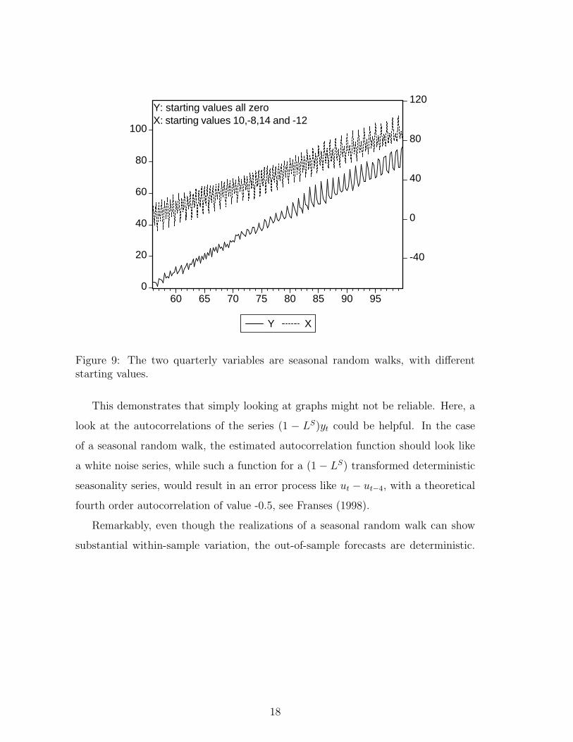
From graphs it is not easy to discern whether a series is a seasonal random walk
or not. The observable pattern depends on the starting values of the time series,
relative to the variance of the error term, see the graphs in Figure 9. When the
starting values are very close to each other, seasonal patterns seem to change quite
rapidly (the series y) and when the starting values are far apart, the graph of the x
series suggests that seasonality is close to constant, at least at first sight.
17
0
20
40
60
80
100
-40
0
40
80
120
60 65 70 75 80 85 90 95
Y X
Y: starting values all zeroX: starting values 10,-8,14 and -12
Figure 9: The two quarterly variables are seasonal random walks, with differentstarting values.
This demonstrates that simply looking at graphs might not be reliable. Here, a
look at the autocorrelations of the series (1 − LS)yt could be helpful. In the case
of a seasonal random walk, the estimated autocorrelation function should look like
a white noise series, while such a function for a (1− LS) transformed deterministic
seasonality series, would result in an error process like ut − ut−4, with a theoretical
fourth order autocorrelation of value -0.5, see Franses (1998).
Remarkably, even though the realizations of a seasonal random walk can show
substantial within-sample variation, the out-of-sample forecasts are deterministic.
18
Indeed, at time n, these forecasts are
yn+1 = yn+1−S
yn+2 = yn+2−S
:
yn+S = yn
yn+S+1 = yn+1
yn+S+2 = yn+2.
Another way of allowing for seasonal random walk type changing pattern, is to
introduce changing parameters. For example, a subtle form of changing seasonality
is described by a time-varying seasonal dummy parameter model. For example, for
S = 4 this model could look like
yt =4∑
s=1
δs,tDs,t + ut, (15)
where
δs,t = δs,t−S + εs,t. (16)
When the variance of εs,t = 0, the constant parameter model appears. The amount
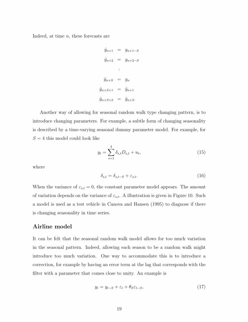
of variation depends on the variance of εs,t. A illustration is given in Figure 10. Such
a model is used as a test vehicle in Canova and Hansen (1995) to diagnose if there
is changing seasonality in time series.
Airline model
It can be felt that the seasonal random walk model allows for too much variation
in the seasonal pattern. Indeed, allowing each season to be a random walk might
introduce too much variation. One way to accommodate this is to introduce a
correction, for example by having an error term at the lag that corresponds with the
filter with a parameter that comes close to unity. An example is
yt = yt−S + εt + θSεt−S, (17)
19
-30
-20
-10
0
10
20
-20
-10
0
10
20
60 65 70 75 80 85 90 95
Y X
X: constant parametersY: parameter for season 1 is random walk
Figure 10: Time series with constant seasonality (x) and with one seasonal dummyparameter as a seasonal random walk (y)
where θS can approximate -1. Bell (1987) demonstrates that when θS = −1, the
model reduces to
yt =S∑
s=1
δsDs,t + εt. (18)
Clearly, this also gives an opportunity to test if there is constant or changing sea-
sonality.
An often applied model, popularized by Box and Jenkins (1970) and named after
its application to monthly airline passenger data, is the airline model. It builds on
the above model by considering
(1− L)(1− LS)yt = (1 + θ1L)(1 + θSLS)εt, (19)
where it should be noted that
(1− L)(1− LS)yt = yt − yt−1 − yt−S + yt−S−1. (20)
This model is assumed to effectively handle a trend in the data using the filter (1−L)
and any changing seasonality using (1 − LS). Strictly speaking, the airline model
20
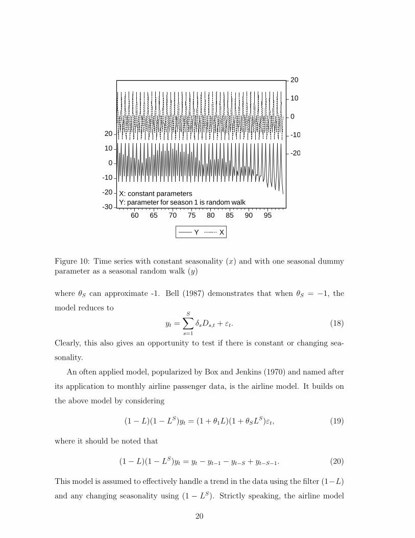
Dependent Variable: LC-LC(-1)-LC(-4)+LC(-5)Method: Least SquaresDate: 04/07/04 Time: 09:48Sample(adjusted): 1981:2 2001:2Included observations: 81 after adjusting endpointsConvergence achieved after 10 iterationsBackcast: 1980:1 1981:1
Variable Coefficient Std. Error t-Statistic Prob.
C -0.000329 0.000264 -1.246930 0.2162MA(1) -0.583998 0.088580 -6.592921 0.0000
SMA(4) -0.591919 0.090172 -6.564320 0.0000
R-squared 0.444787 Mean dependent var -5.01E-05Adjusted R-squared 0.430550 S.D. dependent var 0.016590S.E. of regression 0.012519 Akaike info criterion -5.886745Sum squared resid 0.012225 Schwarz criterion -5.798061Log likelihood 241.4132 F-statistic 31.24325Durbin-Watson stat 2.073346 Prob(F-statistic) 0.000000
Inverted MA Roots .88 .58 .00+.88i -.00 -.88i -.88
Figure 11: Airline model estimation results: quarterly log(consumption) in Japan
assumes S + 1 unit roots. This is due to the fact that the characteristic equation of
the AR part, which is,
(1− z)(1− zS) = 0, (21)
has S + 1 solutions on the unit circle. For example, if S = 4 the solutions are (1,
1, -1, i, -i). This implies a substantial amount of random walk like behavior, even
though it is corrected to some extent by the (1+θ1L)(1+θSLS)εt part of the model.
In terms of forecasting, it assumes very wide confidence intervals around the point
forecasts. On the other hand, the advantages of this model are that it contains only
two parameters and that it can describe a wide range of variables, which can be
observed from the Eviews output in Figures 11, 12 en 13. The estimated residuals
of these models do not obviously indicate mis-specification. On the other hand, it is
clear that the roots of the MA polynomial (indicated at the bottom panel of these
graphs) are close to the unit circle.
21
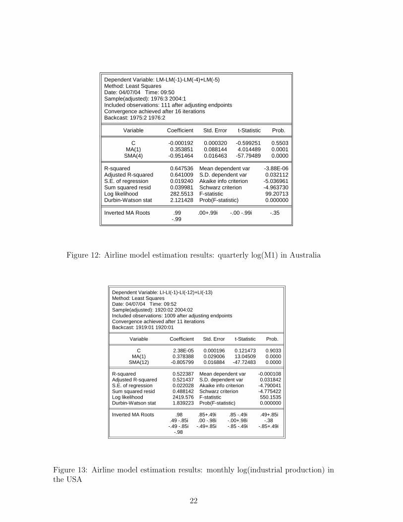
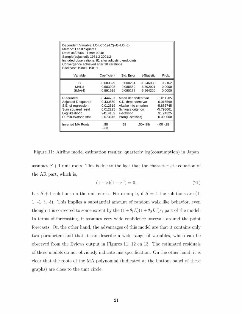
Dependent Variable: LM-LM(-1)-LM(-4)+LM(-5)Method: Least SquaresDate: 04/07/04 Time: 09:50Sample(adjusted): 1976:3 2004:1Included observations: 111 after adjusting endpointsConvergence achieved after 16 iterationsBackcast: 1975:2 1976:2
Variable Coefficient Std. Error t-Statistic Prob.
C -0.000192 0.000320 -0.599251 0.5503MA(1) 0.353851 0.088144 4.014489 0.0001
SMA(4) -0.951464 0.016463 -57.79489 0.0000
R-squared 0.647536 Mean dependent var -3.88E-06Adjusted R-squared 0.641009 S.D. dependent var 0.032112S.E. of regression 0.019240 Akaike info criterion -5.036961Sum squared resid 0.039981 Schwarz criterion -4.963730Log likelihood 282.5513 F-statistic 99.20713Durbin-Watson stat 2.121428 Prob(F-statistic) 0.000000
Inverted MA Roots .99 .00+.99i -.00 -.99i -.35 -.99
Figure 12: Airline model estimation results: quarterly log(M1) in Australia
Dependent Variable: LI-LI(-1)-LI(-12)+LI(-13)Method: Least SquaresDate: 04/07/04 Time: 09:52Sample(adjusted): 1920:02 2004:02Included observations: 1009 after adjusting endpointsConvergence achieved after 11 iterationsBackcast: 1919:01 1920:01
Variable Coefficient Std. Error t-Statistic Prob.
C 2.38E-05 0.000196 0.121473 0.9033MA(1) 0.378388 0.029006 13.04509 0.0000
SMA(12) -0.805799 0.016884 -47.72483 0.0000
R-squared 0.522387 Mean dependent var -0.000108Adjusted R-squared 0.521437 S.D. dependent var 0.031842S.E. of regression 0.022028 Akaike info criterion -4.790041Sum squared resid 0.488142 Schwarz criterion -4.775422Log likelihood 2419.576 F-statistic 550.1535Durbin-Watson stat 1.839223 Prob(F-statistic) 0.000000
Inverted MA Roots .98 .85+.49i .85 -.49i .49+.85i .49 -.85i .00 -.98i -.00+.98i -.38 -.49 -.85i -.49+.85i -.85 -.49i -.85+.49i -.98
Figure 13: Airline model estimation results: monthly log(industrial production) inthe USA
22
Basic structural model
Finally, a model that takes a position in between seasonal adjustment and the airline
model is the Structural Time Series Model, see Harvey (1989). The basic idea is that
a time series can be decomposed in various components, which reflect seasonality,
trend, cycles and so on. This representation facilitates the explicit consideration of
a trend component or a seasonal component, which, if one intends to do so, can
be subtracted from the data to get a trend-free or seasonality-free series. Often, a
Structural Time Series Model can be written as a seasonal ARIMA type model, and
hence, its descriptive quality is close to that of a seasonal ARIMA model.
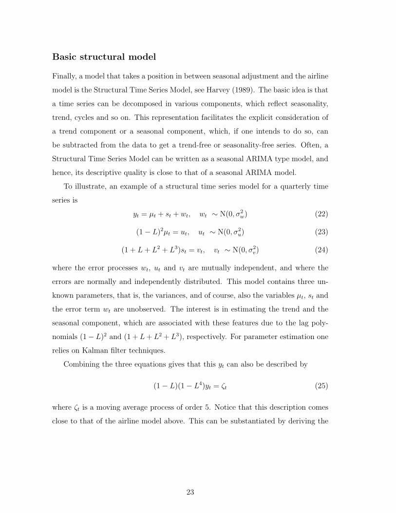
To illustrate, an example of a structural time series model for a quarterly time
series is
yt = µt + st + wt, wt ∼ N(0, σ2w) (22)
(1− L)2µt = ut, ut ∼ N(0, σ2u) (23)
(1 + L + L2 + L3)st = vt, vt ∼ N(0, σ2v) (24)
where the error processes wt, ut and vt are mutually independent, and where the
errors are normally and independently distributed. This model contains three un-
known parameters, that is, the variances, and of course, also the variables µt, st and
the error term wt are unobserved. The interest is in estimating the trend and the
seasonal component, which are associated with these features due to the lag poly-
nomials (1−L)2 and (1 + L + L2 + L3), respectively. For parameter estimation one
relies on Kalman filter techniques.
Combining the three equations gives that this yt can also be described by
(1− L)(1− L4)yt = ζt (25)
where ζt is a moving average process of order 5. Notice that this description comes
close to that of the airline model above. This can be substantiated by deriving the
23
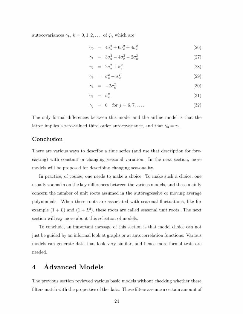
autocovariances γk, k = 0, 1, 2, . . ., of ζt, which are
γ0 = 4σ2u + 6σ2
v + 4σ2w (26)
γ1 = 3σ2u − 4σ2
v − 2σ2w (27)
γ2 = 2σ2u + σ2
v (28)
γ3 = σ2u + σ2
w (29)
γ4 = −2σ2w (30)
γ5 = σ2w (31)
γj = 0 for j = 6, 7, . . . . (32)
The only formal differences between this model and the airline model is that the
latter implies a zero-valued third order autocovariance, and that γ3 = γ5.
Conclusion
There are various ways to describe a time series (and use that description for fore-
casting) with constant or changing seasonal variation. In the next section, more
models will be proposed for describing changing seasonality.
In practice, of course, one needs to make a choice. To make such a choice, one
usually zooms in on the key differences between the various models, and these mainly
concern the number of unit roots assumed in the autoregressive or moving average
polynomials. When these roots are associated with seasonal fluctuations, like for
example (1 + L) and (1 + L2), these roots are called seasonal unit roots. The next
section will say more about this selection of models.
To conclude, an important message of this section is that model choice can not
just be guided by an informal look at graphs or at autocorrelation functions. Various
models can generate data that look very similar, and hence more formal tests are
needed.
4 Advanced Models
The previous section reviewed various basic models without checking whether these
filters match with the properties of the data. These filters assume a certain amount of
24
unit roots, and it seems sensible to test whether these roots are present or not. In this
section I discuss models that allow for a more sophisticated description of seasonal
patterns, while allowing for the possible presence of zero frequency trends. Next, I
will discuss models that allow the trend and season variation to be intertwined.
Seasonal unit roots
A time series variable has a non-seasonal unit root if the autoregressive polynomial
(of the model that best describes this variable), contains the component 1− L, and
the moving-average part does not. For example, the model yt = yt−1 + εt has a
first-order autoregressive polynomial 1 − L, as it can be written as (1 − L)yt = εt.
Hence, data that can be described by the random walk model are said to have a unit
root. The same holds of course for the model yt = µ + yt−1 + εt, which is a random
walk with drift. Solving this last model to the first observation, that is,
yt = y0 + µt + εt + εt−1 + · · ·+ ε1 (33)
shows that such data also have a deterministic trend. Due to the summation of the
error terms, it is possible that data diverge from the overall trend µt for a long time,
and hence one could conclude from a graph that there are all kinds of trends with
directions that vary from time to time. Therefore, such data are sometimes said to
have a stochastic trend.
The unit roots in seasonal data, which can be associated with changing season-
ality, are seasonal unit roots, see Hylleberg et al. (1990) [HEGY]. For quarterly
data, these roots are −1, i, and -i. For example, data generated from the model
yt = −yt−1 + εt would display seasonality, but if one were to make graphs with the
split seasonals, then one could observe that the quarterly data within a year shift
places quite frequently. Similar observations hold for the model yt = −yt−2 + εt,
which can be written as (1 + L2)yt = εt, where the autoregressive polynomial 1 + L2
corresponds to the seasonal unit roots i and -i, as these two values solve the equation
1 + z2 = 0.
25
Testing for seasonal unit roots
In contrast to simply imposing (seasonal) unit roots, one can also test whether they
are present or not. The most commonly used method for this purpose is the HEGY
method. For quarterly data it amounts to a regression of ∆4yt on deterministic
terms like an intercept, seasonal dummies, a trend and seasonal trends and on (1 +
L + L2 + L3)yt−1, (−1 + L − L2 + L3)yt−1, −(1 + L2)yt−1, −(1 + L2)yt−2, and on
lags of ∆4yt. A t−test is used to examine the significance of the parameter for
(1 + L + L2 + L3)yt−1, and similarly, a t−test for (−1 + L−L2 + L3)yt−1 and a joint
F−test for −(1+L2)yt−1 and −(1+L2)yt−2 . An insignificant test value indicates the
presence of the associated root(s), which are 1, −1, and the pair i, −i, respectively.
Asymptotic theory for the tests is developed in Hylleberg et al. (1990), and useful
extensions are put forward in Smith and Taylor (1998).
When including deterministic terms, it is important to recall the discussion in
Section 2, concerning the seasonal dummies. Indeed, when the seasonal dummies are
included unrestrictedly, it is possible that the time series (under the null hypothesis
of seasonal unit roots) can display seasonally varying deterministic trends. Hence,
when checking for example whether the (1+L) filter can be imposed, one also needs
to impose that the α2 parameter for cos(πt) in (11) equals zero. The preferable way
to include deterministics therefore is to include the alternating dummy variables
D1,t −D2,t + D3,t −D4,t, D1,t −D3,t, and D2,t −D4,t. And, for example, under the
null hypothesis that there is a unit root −1, the parameter for the first alternating
dummy should also be zero. These joint tests extend the work of Dickey and Fuller
(1981), and are discussed in Smith and Taylor (1999). When models are created
for panels of time series or for multivariate series, as I will discuss below, these
restrictions on the deterministics (based on the sine-cosine notation) are important
too.
Kawasaki and Franses (2003) propose to detect seasonal unit roots within the
context of a structural time series model. They rely on model selection criteria. Us-
ing Monte Carlo simulations, they show that the method works well. They illustrate
their approach for several quarterly macroeconomic time series variables.
26
Seasonal cointegration
In case two or more seasonally observed time series have seasonal unit roots, one
may be interested in testing for common seasonal unit roots, that is, in testing for
seasonal cointegration. If these series have such roots in common, they will have
common changing seasonal patterns.
Engle et al. (1993) [EGHL] propose a two-step method to see if there is seasonal
cointegration. When two series y1,t and y2,t have a common non-seasonal unit root,
then the series ut defined by
ut = (1 + L + L2 + L3)y1,t − α1(1 + L + L2 + L3)y2,t (34)
does not need the (1− L) filter to become stationary. Seasonal cointegration at the
annual frequency π, corresponding to unit root −1, implies that
vt = (1− L + L2 − L3)y1,t − α2(1− L + L2 − L3)y2,t (35)
does not need the (1 + L) differencing filter. And, seasonal cointegration at the
annual frequency π/2, corresponding to the unit roots ±i, means that
wt = (1− L2)y1,t − α3(1− L2)y2,t − α4(1− L2)y1,t−1 − α5(1− L2)y2,t−1 (36)
does not have the unit roots ±i. In case all three ut, vt and wt do not have the
relevant unit roots, the first equation of a simple version of a seasonal cointegration
model is
∆4y1,t = γ1ut−1 + γ2vt−1 + γ3wt−2 + γ4wt−3 + ε1,t, (37)
where γ1 to γ4 are error correction parameters. The test method proposed in EGHL
is a two-step method, similar to the Engle-Granger (1987) approach to non-seasonal
time series.
Seasonal cointegration in a multivariate time series Yt can also be analyzed us-
ing an extension of the Johansen approach, see Johansen and Schaumburg (1999),
Franses and Kunst (1999a). It amounts to testing the ranks of matrices that corre-
spond to variables which are transformed using the filters to remove the roots 1, -1
or ± i. More precise, consider the (m× 1) vector process Yt, and assume that it can
27
be described by the VAR(p) process
Yt = ΘDt + Φ1Yt−1 + · · ·+ ΦpYt−p + et, (38)
where Dt is the (4 × 1) vector process Dt = (D1,t, D2,t, D3,t, D4,t)′ containing the
seasonal dummies, and where Θ is an (m × 4) parameter matrix. Similar to the
Johansen (1995) approach and conditional on the assumption that p > 4, the model
can be rewritten as
∆4Yt = ΘDt + Π1Y1,t−1 (39)
+ Π2Y2,t−1 + Π3Y3,t−2 + Π4Y3,t−1 (40)
+ Γ1∆4Yt−1 + · · ·+ Γp−4∆4Yt−(p−4) + et,
where
Y1,t = (1 + L + L2 + L3)Yt
Y2,t = (1− L + L2 − L3)Yt
Y3,t = (1− L2)Yt.
This is a multivariate extension of the univariate HEGY model. The ranks of the
matrices Π1, Π2, Π3 and Π4 determine the number of cointegration relations at each
of the frequencies. Again, it is important to properly account for the deterministics,
in order not to have seasonally diverging trends, see Franses and Kunst (1999a) for
a solution.
Periodic models
An alternative class of models is the periodic autoregression. Consider a univariate
time series yt, which is observed quarterly for N years. It is assumed that n = 4N .
A periodic autoregressive model of order p [PAR(p)] can be written as
yt = µs + φ1syt−1 + · · ·+ φpsyt−p + εt, (41)
or
φp,s(L)yt = µs + εt, (42)
28
with
φp,s(L) = 1− φ1sL− · · · − φpsLp, (43)
where µs is a seasonally-varying intercept term. The φ1s, . . . , φps are autoregressive
parameters up to order ps which may vary with the season s, where s = 1, 2, 3, 4.
For εt it can be assumed it is a standard white noise process with constant variance
σ2, but that may be relaxed by allowing εt to have seasonal variance σ2s . As some
φis, i = 1, 2, . . . , p, can take zero values, the order p is the maximum of all ps.
Multivariate representation
In general, the PAR(p) process can be rewritten as an AR(P ) model for the (4 ×1) vector process YT = (Y1,T , Y2,T , Y3,T , Y4,T )′, T = 1, 2, . . . , N , where Ys,T is the
observation of yt in season s of year T . The model is then
Φ0YT = µ + Φ1YT−1 + · · ·+ ΦP YT−P + εT , (44)
or
Φ(L)YT = µ + εT , (45)
with
Φ(L) = Φ0 − Φ1L− · · · − ΦP LP , (46)
µ = (µ1, µ2, µ3, µ4)′, εT = (ε1,T , ε2,T , ε3,T , ε4,T )′, and εs,T is the observation on the
error process εt in season s of year T . The lag operator L applies to data at frequen-
cies t and to T , that is, Lyt = yt−1 and LYT = YT−1. The Φ0, Φ1, . . . , ΦP are 4 × 4
parameter matrices with elements
Φ0[i, j] =
1 i = j,0 j > i,−φi−j,i i < j,
(47)
Φk[i, j] = φi+4k−j,i, (48)
for i = 1, 2, 3, 4, j = 1, 2, 3, 4, and k = 1, 2, . . . , P . For P it holds that P =
1+ [(p− 1)/4], where [ · ] is the integer function. Hence, when p is less than or equal
to 4, the value of P is 1.
As Φ0 is a lower triangular matrix, model (44) is a recursive model. This means
that Y4,T depends on Y3,T , Y2,T , and Y1,T , and on all variables in earlier years.
29
Similarly, Y3,T depends on Y2,T and Y1,T , and Y2,T on Y1,T and on all observations in
past years. As an example, consider the PAR(2) process
yt = φ1syt−1 + φ2syt−2 + εt, (49)
which can be written as
Φ0YT = Φ1YT−1 + εT , (50)
with
Φ0 =
1 0 0 0−φ12 1 0 0−φ23 −φ13 1 0
0 −φ24 −φ14 1
and Φ1 =
0 0 φ21 φ11
0 0 0 φ22
0 0 0 00 0 0 0
. (51)
A useful representation is based on the possibility of decomposing a non-periodic
AR(p) polynomial as (1 − α1L)(1 − α2L) · · · (1 − αpL), see Boswijk, Franses and
Haldrup (1997) where this representation is used to test for (seasonal) unit roots
in periodic models. Note that this can only be done when the solutions to the
characteristic equation for this AR(p) polynomial are all real-valued. Similar results
hold for the multivariate representation of a PAR(p) process, and it can be useful
to rewrite (44) asP∏
i=1
Ξi(L)YT = µ + εT , (52)
where the Ξi(L) are 4× 4 matrices with elements which are polynomials in L.
A simple example is the PAR(2) process
Ξ1(L)Ξ2(L)YT = εT , (53)
with
Ξ1(L) =
1 0 0 −β1L−β2 1 0 00 −β3 1 00 0 −β4 1
,
Ξ2(L) =
1 0 0 −α1L−α2 1 0 0
0 −α3 1 00 0 −α4 1
. (54)
30
This PAR(2) model can be written as
(1− βsL)(1− αsL)yt = µs + εt, . (55)
or
yt − αsyt−1 = µs + βs(yt−1 − αs−1yt−2) + εt, (56)
as, and this is quite important, the lag operator L also operates on αs, that is,
Lαs = αs−1 for all s = 1, 2, 3, 4 and with α0 = α4. The characteristic equation is
|Ξ1(z)Ξ2(z)| = 0, (57)
and this is equivalent to
(1− β1β2β3β4z)(1− α1α2α3α4z) = 0. (58)
So, the PAR(2) model has one unit root when either β1β2β3β4 = 1 or α1α2α3α4 = 1,
and has at most two unit roots when both products equal unity. The case where
α1α2α3α4 = 1 while not all αs are equal to 1 is called periodic integration, see
Osborn (1988) and Franses (1996). Tests for periodic integration are developed in
Boswijk and Franses (1996) for the case without allowing for seasonal unit roots, and
in Boswijk, Franses and Haldrup (1997) for the case where seasonal unit roots can
also occur. Obviously, the maximum number of unity solutions to the characteristic
equation of a PAR(p) process is equal to p.
The analogy of a univariate PAR process with a multivariate time series process
can be used to derive explicit formulae for one- and multi-step ahead forecasting, see
Franses (1996). It should be noted that then the one-step ahead forecasts concern
one-year ahead forecasts for all four Ys,T series. For example, for the model YT =
Φ−10 Φ1YT−1 + ωT , where ωT = Φ−1
0 εT , the forecast for N + 1 is YN+1 = Φ−10 Φ1YN .
Finally, one may wonder what the consequences are of fitting non-periodic models
to periodic data. One consequence is that such a non-periodic model requires many
lags, see Franses and Paap (2004) and Del Barrio Castro and Osborn (2004). For
example, a PAR(1) model can be written as
yt = αs+3αs+2αs+1αsyt−4 + εt + αs+3εt−1 + αs+3αs+2εt−2 + αs+3αs+2αs+1εt−3. (59)
31
As αs+3αs+2αs+1αs is equal for all seasons, the AR parameter at lag 4 in a non-
periodic model is truly non-periodic, but of course, the MA part is not. The MA
part of this model is of order 3. If one estimates a non-periodic MA model for these
data, the MA parameter estimates will attain an average value of the αs+3, αs+3αs+2,
and αs+3αs+2αs+1 across the seasons. In other words, one might end up considering
an ARMA(4,3) model for PAR(1) data. And, if one decides not to include an MA
part in the model, one usually needs to increase the order of the autoregression to
whiten the errors. This suggests that higher-order AR models might fit to low-order
periodic data. When αs+3αs+2αs+1αs = 1, one has a high-order AR model for the ∆4
transformed time series. In sum, there seems to be a trade-off between seasonality
in parameters and short lags against no seasonality in parameters and longer lags.
Conclusion
There is a voluminous literature on formally testing for seasonal unit roots in non-
periodic data and on testing for unit roots in periodic autoregressions. There are
many simulation studies to see which method is best. Also, there are many studies
which examine whether imposing seasonal unit roots or not, or assuming unit roots
in periodic models or not, lead to better forecasts. This also extends to the case
of multivariate series, where these models allow for seasonal cointegration or for
periodic cointegration. An example of a periodic cointegration model is
∆4yt = γs(yt−4 − βsxt−4) + εt, (60)
where γs and βs can take seasonally varying values, see Boswijk and Franses (1995).
For example, Lof and Franses (2001) analyze periodic and seasonal cointegration
models for bivariate quarterly observed time series in an empirical forecasting study,
as well as a VAR model in first differences, with and without cointegration restric-
tions, and a VAR model in annual differences. The VAR model in first differences
without cointegration is best if one-step ahead forecasts are considered. For longer
forecast horizons, the VAR model in annual differences is better. When compar-
ing periodic versus seasonal cointegration models, the seasonal cointegration models
tend to yield better forecasts. Finally, there is no clear indication that multiple
32
equations methods improve on single equation methods.
To summarize, tests for periodic variation in the parameters and for unit roots
allow one to make a choice between the various models for seasonality. There are
many tests around, and they are all easy to use. Not unexpectedly, models and
methods for data with frequencies higher than 12 can become difficult to use in
practice, see Darne (2004) for a discussion of seasonal cointegration in monthly
series. Hence, here there is a need for more future research.
5 Recent advances
This section deals with a few recent developments in the area of forecasting seasonal
time series. These are (i) seasonality in panels of time series, (ii) periodic models
for financial series, and (iii) nonlinear models for seasonal time series.
Seasonality in panels of time series
The search for common seasonal patterns can lead to a dramatic reduction in the
number of parameters, see Engle and Hylleberg (1996). One way to look for common
patterns across the series yi,t, where i = 1, 2, .., I, and I can be large, is to see of the
series have common dynamics or common trends. Alternatively, one can examine if
series have common seasonal deterministics.
As can be understood from the discussion on seasonal unit roots, before one can
say something about (common) deterministic seasonality, one first has to decide on
the number of seasonal unit roots. The HEGY test regression for seasonal unit roots
is
Φpi(L)∆4yi,t = µi,t + ρi,1S(L)yi,t−1 + ρi,2A(L)yi,t−1
+ ρi,3∆2yi,t−1 + ρi,4∆2yi,t−2 + εt, (61)
and now it is convenient to take
µi,t = µi + α1,i cos(πt) + α2,i cos(πt
2) + α3,i cos(
π(t− 1)
2) + δit, (62)
and where ∆k is the k−th order differencing filter, S(L)yi,t = (1 + L + L2 + L3)yi,t
and A(L)yi,t = −(1 − L + L2 − L3)yi,t. The model assumes that each series yi,t
33
can be described by a (pi + 4)−th order autoregression. Smith and Taylor (1999)
and Franses and Kunst (1999a,b) argue that an appropriate test for a seasonal unit
root at the bi-annual frequency is now given by a joint F−test for ρi,2 and α1,i. An
appropriate test for the two seasonal unit roots at the annual frequency is then given
by a joint F−test for ρ3,i, ρ4,i, α2,i and α3,i. Franses and Kunst (1999b) consider
these F -tests in a model where the autoregressive parameters are pooled over the
equations, hence a panel HEGY test. The power of this panel test procedure is rather
large. Additionally, once one has taken care off seasonal unit roots, these authors
examine if two or more series have the same seasonal deterministic fluctuations. This
can be done by testing for cross-equation restrictions.
Periodic GARCH
Periodic models might also be useful for financial time series. They can be used
not only to describe the so-called day-of-the-week effects, but also to describe the
apparent differences in volatility across the days of the week. Bollerslev and Ghysels
(1996) propose a periodic generalized autoregressive conditional heteroskedasticity
(PGARCH) model. Adding a periodic autoregression for the returns to it, one has
a PAR(p)-PGARCH(1,1) model, which for a daily observed financial time series yt,
t = 1, . . . , n = 5N , can be represented by
xt = yt −5∑
s=1
(µs +
p∑i=1
φisyt−i
)Ds,t
=√
htηt (63)
with ηt ∼ N(0, 1) for example, and
ht =5∑
s=1
(ωs + ψsx2t−1)Ds,t + γht−1, (64)
where the xt denotes the residual of the PAR model for yt, and where Ds,t denotes
a seasonal dummy for the day of the week, that is, s = 1, 2, 3, 4, 5.
In order to investigate the properties of the conditional variance model, it is
useful to define zt = x2t − ht, and to write it as
x2t =
5∑s=1
(ωs + (ψs + γ)x2t−1)Ds,t + zt − γzt−1. (65)
34
This ARMA process for x2t contains time-varying parameters ψs+γ and hence strictly
speaking, it is not a stationary process. To investigate the stationarity properties of
x2t , (65) can be written in a time-invariant representation. Franses and Paap (2000)
successfully fit such a model to the daily S&P 500 index, and even find that
Π5s=1(ψs + γ) = 1. (66)
In other words, they fit a periodically integrated GARCH model.
Models of seasonality and nonlinearity
It is well known that a change in the deterministic trend properties of a time series
yt is easily mistaken for the presence of a unit root. In a similar vein, if a change in
the deterministic seasonal pattern is not detected, one might well end up imposing
seasonal unit roots, see Ghysels (1994), Smith and Otero (1997), Franses, Hoek and
Paap (1997) and Franses and Vogelsang (1998).
Changes in deterministic seasonal patterns usually are modelled by means of
one-time abrupt and discrete changes. However, when seasonal patterns shift due
to changes in technology, institutions and tastes, for example, these changes may
materialize only gradually. This suggests that a plausible description of time-varying
seasonal patterns is
φ(L)∆1yt =4∑
s=1
δ1,sDs,t(1−G(t; γ, c)) +4∑
s=1
δ2,sDs,tG(t; γ, c) + εt, (67)
where G(t; γ, c) is the logistic function
G(st; γ, c) =1
1 + exp{−γ(st − c)} , γ > 0. (68)
As st increases, the logistic function changes monotonically from 0 to 1, with the
change being symmetric around the location parameter c, as G(c−z; γ, c) = 1−G(c+
z; γ, c) for all z. The slope parameter γ determines the smoothness of the change. As
γ →∞, the logistic function G(st; γ, c) approaches the indicator function I[st > c],
whereas if γ → 0, G(st; γ, c) → 0.5 for all values of st. Hence, by taking st = t,
the model takes an “intermediate” position in between deterministic seasonality and
stochastic trend seasonality.
35
Nonlinear models with smoothly changing deterministic seasonality are proposed
in Franses and van Dijk (2004). These authors examine the forecasting performance
of various models for seasonality and nonlinearity for quarterly industrial produc-
tion series of 18 OECD countries. They find that the accuracy of point forecasts
varies widely across series, across forecast horizons and across seasons. However,
in general, linear models with fairly simple descriptions of seasonality outperform
at short forecast horizons, whereas nonlinear models with more elaborate seasonal
components dominate at longer horizons. Simpler models are also preferable for
interval and density forecasts at short horizons. Finally, none of the models is found
to be the best and hence, forecast combination is worthwhile.
To summarize, recent advances in modeling and forecasting seasonal time series
focus at (i) models for panels of time series and at (ii) models which not only capture
seasonality, but also conditional volatility and non-linearity, for example. To fully
capture all these features is not easy, also as various features may be related. More
research is needed in this area too.
6 Conclusion
Forecasting studies show that model specification efforts pay off in terms of perfor-
mance. Simple models for seasonally differenced data forecast well for one or a few
steps ahead. For longer horizons, more involved models are much better. These
involved models address seasonality in conjunction with trends, non-linearity and
conditional volatility. Much more research is needed to see which models are to be
preferred in which situations.
There are at least two well articulated further research issues. The first concerns
methods to achieve parsimony. Indeed, seasonal time series models for monthly or
weekly data contain a wealth of parameters, and this can reduce efficiency dramat-
ically. The second concerns the analysis of unadjusted data for the situation where
people would want to rely on adjusted data, that is, for decisions on turning points.
How would one draw inference in case trends, cycles and seasonality are related?
Finally, in case one persists in considering seasonally adjusted data, how can we
36

design methods that allow for the best possible interpretation of these data, when
the underlying process has all kinds of features?
It is hoped that this chapter has contributed to get an interest in modeling and
forecasting seasonal time series data, and that it has stimulated an interest in doing
further research in this fascinating area.
37
References
Bell, W. R. and S. C. Hillmer (1984), Issues Involved with the Seasonal Adjust-
ment of Economic Time Series (with discussion), Journal of Business and Economic
Statistics, 2, 291-320.
Bell, W.R. (1987), A Note on Overdifferencing and the Equivalence of Seasonal
Time Series Models With Monthly Means and Models With (0, 1, 1)12 Seasonal Parts
When θ = 1, Journal of Business & Economics Statistics, 5, 383-387.
Bollerslev, T. and E. Ghysels (1996), Periodic Autoregressive Conditional Het-
eroscedasticity, Journal of Business and Economic Statistics, 14, 139-151.
Boswijk, H. P. and P. H. Franses (1995), Periodic Cointegration – Representation
and Inference, Review of Economics and Statistics, 77, 436-454.
Boswijk, H. P. and P. H. Franses (1996), Unit Roots in Periodic Autoregressions,
Journal of Time Series Analysis, 17, 221-245.
Boswijk, H. P., P. H. Franses and N. Haldrup (1997) Multiple Unit Roots in Pe-
riodic Autoregression, Journal of Econometrics, 80, 167-193.
Brendstrup, B., S. Hylleberg, M.O. Nielsen, L. L. Skippers, and L. Stentoft (2004),
Seasonality in Economic Models, Macroeconomic Dynamics, 8, 362-394.
Canova, F. and E. Ghysels (1994), Changes in Seasonal Patterns: Are they Cycli-
cal?, Journal of Economic Dynamics and Control, 18, 1143-1171.
Canova, F. and B. E. Hansen (1995), Are Seasonal Patterns Constant over Time?
A Test for Seasonal Stability, Journal of Business and Economic Statistics, 13, 237-
252.
38
Darne, O. (2004), Seasonal Cointegration for Monthly Data, Economics Letters,
82, 349-356.
Del Barrio Castro, T. and D.R. Osborn (2004), The Consequences of Seasonal Ad-
justment for Periodic Autoregressive Processes, Reconometrics Journals, to appear.
Dickey, D.A. and W.A. Fuller (1981), Likelihood Ratio Statistics for Autoregres-
sive Time Series with a Unit Root, Econometrica, 49, 1057-1072.
Engle, R.F. and C.W.J. Granger (1987), Cointegration and Error Correction: Rep-
resentation, Estimation, and Testing, Econometrica, 55, 251-276.
Engle, R.F. and C.W.J. Granger (1991, eds.), Long-Run Economic Relationships:
Readings in Cointegration, Oxford: Oxford University Press.
Engle, R. F., C. W. J. Granger, S. Hylleberg and H. S. Lee (1993), Seasonal Coin-
tegration: The Japanese Consumption Function, Journal of Econometrics, 55, 275-
298.
Engle, R.F. and S. Hylleberg (1996), Common Seasonal Features: Global Unem-
ployment, Oxford Bulletin of Economics and Statistics, 58, 615-630.
Findley, D.F., B.C. Monsell, W.R. Bell, M.C. Otto, and B.-C. Chen (1998), New
Capabilities and Methods of the X-12-ARIMA Seasonal-Adjustment Program (with
Discussion), Journal of Business and Economic Statistics 16, 127-177.
Franses, P. H. (1991), A Multivariate Approach to Modeling Univariate Seasonal
Time Series, Econometric Institute Report 9101, Erasmus University Rotterdam.
Franses, P. H. (1994), A Multivariate Approach to Modeling Univariate Seasonal
39
Time Series, Journal of Econometrics, 63, 133-151.
Franses, P.H. (1996), Periodicity and Stochastic Trends in Economic Time Series,
Oxford: Oxford University Press.
Franses, P.H. (1998), Time Series Models for Business and Economic Forecasting,
Cambridge: Cambridge University Press.
Franses, P.H. (2001), Some Comments on Seasonal Adjustment, Revista De Econo-
mia del Rosario (Bogota, Colombia), 4, 9-16.
Franses, P. H., H. Hoek and R. Paap (1997), Bayesian Analysis of Seasonal Unit
Roots and Seasonal Mean Shifts, Journal of Econometrics, 78, 359-380.
Franses, P. H. and S. Hylleberg and H. S. Lee (1995), Spurious Deterministic Sea-
sonality, Economics Letters, 48, 249-256.
Franses, P. H. and R.M. Kunst (1999a), On the Role of Seasonal Intercepts in
Seasonal Cointegration, Oxford Bulletin of Economics and Statistics, 61, 409-433.
Franses, P.H. and R.M. Kunst (1999b), Testing Common Deterministic Seasonal-
ity, with an Application to Industrial Production, Econometric Institute Report
9905, Erasmus University Rotterdam.
Franses, P. H. and R. Paap (2000), Modelling Day-of-the-week Seasonality in the
S&P 500 Index, Applied Financial Economics, 10, 483-488.
Franses P.H. and R. Paap (2004), Periodic Time Series Models, Oxford: Oxford
University Press.
Farnses, P.H. and D.J.C. van Dijk (2000), Non-linear Time Series Models in Em-
40
pirical Finance, Cambridge: Cambridge University Press.
Franses, P.H. and D.J.C. van Dijk (2004), The Forecasting Performance of Vari-
ous Models for Seasonality and Nonlinearity for Quarterly Industrial Production,
International Journal of Forecasting, to appear.
Franses, P. H. and T. J. Vogelsang (1998), On Seasonal Cycles, Unit Roots and
Mean Shifts, Review of Economics and Statistics, 80, 231-240.
Ghysels, E. (1994), On the Periodic Structure of the Business Cycle, Journal of
Business and Economic Statistics, 12, 289-298.
Ghysels, E., C.W.J. Granger and P.L. Siklos (1996), Is Seasonal Adjustment a Lin-
ear or a Nnnlinear Data-Filtering Process? (with Discussion), Journal of Business
and Economic Statistics 14, 374-397.
Ghysels, E. and D. R. Osborn (2001), The Econometric Analysis of Seasonal Time
Series, Cambridge: Cambridge University Press.
Granger, C.W.J. and T. Terasvirta (1993), Modelling Non-Linear Economic Re-
lationships, Oxford: Oxford University Press.
Harvey, A.C. (1989), Forecasting, Structural Time Series Models and the Kalman
Filter, Cambridge: Cambridge University Press.
Haugen, R.A. and J. Lakonishok (1987), The Incredible January Effect: The Stock
Market’s Unsolved Mystery, New York: McGraw-Hill.
Hylleberg, S. (1986), Seasonality in regression, Orlando: Academic Press.
Hylleberg, S. (1992), Modelling Seasonality, Oxford: Oxford University Press.
41
Hylleberg, S., R. F. Engle, C. W. J. Granger, and B. S. Yoo (1990), Seasonal Inte-
gration and Cointegration, Journal of Econometrics, 44, 215-238.
Johansen, S. (1995), Likelihood-Based Inference in Cointegrated Vector Autoregres-
sive Models, Oxford: Oxford University Press.
Johansen, S. and E. Shaumburg, (1999), Likelihood Analysis of Seasonal Cointe-
gration, Journal of Econometrics, 88, 301-339.
Kawasaki, Y. and P.H. Franses (2003), Detecting Seasonal Unit Roots in a Struc-
tural Time Series Model, Journal of Applied Statistics, 30, 373-387.
Koopman, S.J. and P.H. Franses (2003), Constructing Seasonally Adjusted Data
with Time-Varying Confidence Intervals, Oxford Bulletin of Economics and Statis-
tics, 64, 509-526.
Lof, M. and P. H. Franses (2001), On Forecasting Cointegrated Seasonal Time Se-
ries, International Journal of Forecasting, 17, 607-621.
Maravall, A. (1995), Unobserved Components in Economic Time Series, in H. Pe-
saran, P. Schmidt and M. Wickens (eds.), Handbook of Applied Econometrics (Vol-
ume 1), Oxford: Basil Blackwell.
Ooms, M. and P.H. Franses (1997), On Periodic Correlations between Estimated
Seasonal and Nonseasonal Components in German and US Unemployment, Journal
of Business and Economic Statistics 15, 470-481.
Osborn, D. R. (1988), Seasonality and Habit Persistence in a Life-Cycle Model of
Consumption, Journal of Applied Econometrics, 3, 255-266.
42
Osborn, D. R. (1990), A Survey of Seasonality in UK Macroeconomic Variables,
International Journal of Forecasting, 6, 327-336.
Osborn, D. R. (1991), The Implications of Periodically Varying Coefficients for Sea-
sonal Time-Series Processes, Journal of Econometrics, 48, 373-384.
Osborn, D. R. and P. M. M. Rodrigues (2001), Asymptotic Distributions of Sea-
sonal Unit Root Tests: A Unifying Approach, Econometric Reviews, 21, 221-241.
Shiskin, J. and H. Eisenpress (1957), Seasonal Adjustment by Electronic Computer
Methods, Journal of the American Statistical Association 52, 415-449.
Smith, J. and J. Otero (1997), Structural Breaks and Seasonal Integration, Eco-
nomics Letters, 56, 13-19.
Smith, R.J. and A.M.R. Taylor (1998), Additional Critical Values and Asymptotic
Representations for Seasonal Unit Root Tests, Journal of Econometrics, 85, 269-288.
Smith, R. J. and A. M. R. Taylor (1999), Likelihood Ratio Tests for Seasonal Unit
Roots, Journal of Time Series Analysis, 20, 453-476.
43