Forecasting recessions in real time∗

Knut Are Aastveit† Anne Sofie Jore‡ Francesco Ravazzolo§

October 7, 2013

Abstract

This paper reviews several methods to define and forecast classical business cycle

turning points in Norway, a country which does not have an official business cycle

indicator. It compares the Bry and Boschan rule (BB), an autoregressive Markov

Switching model (MS), and their versions augmented with surveys or financial indi-

cators, using several vintages of Norwegian Gross Domestic Product as the business

cycle indicator. Timing of the business cycles depends on the vintage and the

method used. BB provides the most reliable definition of business cycles. A fore-

casting exercise is also presented: the BB applied to density forecasts augmented

with the consumer confidence survey, the regional network survey, and the financial

condition index provides the most timely predictions for Norwegian turning points

in real time.

JEL-codes: C32, C52, C53, E37, E52

Keywords: Density combination; Forecast densities; Turning Points; Real-time data

∗We thank Hilde Bjørnland, James Mitchell, Christie Smith, Leif Anders Thorsrud and Shaun Vahey

for helpful comments and their work in SAM at early stages. We also thank seminar and conference

participants at the workshop on “New Methods for Forecasting Macroeconomic Data” at the University of

Nottingham, in particular our discussant Nicholas Fawcett, at The 32nd Annual International Symposium

on Forecasting, at the 2012 Computational and Financial Econometrics conference, and at Norges Bank.

The views expressed in this paper are those of the authors and should not be attributed to Norges Bank.†Norges Bank, Knut-Are.Aastveit@norges-bank.no‡Corresponding author : Norges Bank, Anne-Sofie.Jore@norges-bank.no§Norges Bank and BI Norwegian Business School, Francesco.Ravazzolo@norges-bank.no

1

1 Introduction

Short-term analysis in central banks and other policy institutions is intended to provide

policy makers, and possible a larger audience, with assessments of the recent past and

current business cycle. Point and density forecasts of few variables of interest are often

provided. However, the analysis of current economic conditions do not rely just on this

information, and there is a long tradition in business cycle analysis and related research

on separating periods with contraction with periods with expansion, see Schumpeter

(1954). Policy decisions vary depending on the fact the economy is in an expansion or

recession period. Most of the research has focused on US data, where the NBER cycle

is the official and often defined reference cycle. But many other countries do not have

an official dating and, for example, a Norwegian classical business cycles does not exist.

In this paper we review several methods to define classical business cycle turning

points for the Norwegian economy. The Norwegian business cycle is not fully synchro-

nized with cycles of other Scandinavian countries, nor either with the European cycle

and/or US cycle for several reasons, including Norway is a small open economy with

large exports of energy (gas and oil) goods. We compare a Bry and Boschan rule (BB)

as in Harding and Pagan (2002) and an autoregressive Markov Switching model (MS)

as in Hamilton (1989), all two methods applied to an univariate series, the Norwegian

Gross Domestic Product (GDP).

Macroeconomic data, and in particular GDP, are subject to important revisions over

time. Benchmark revisions, but also revisions due to new information change series

substantially and for several years. Economic decisions (see Orphanides and van Norden

(2002)) are not immune to such changes. Hamilton (2011) also shows that business

cycle dating can result in important differences when several vintages are considered.

We compare business cycle turning points given by the three methods listed above when

using 2012 ex-post revised data to real-time data.

Finally, data are released with substantial delays and therefore economic decisions

rely on forecasts of the missing recent information. The literature on point forecast is

2

large (see Timmermann (2006) for a recent review), it is growing on density forecasting,

but it is very thin on turning point prediction, see e.g. Billio et al. (2012). Markov

switching models can produce point, density and turning point forecasts; on contrary, the

BB rule must be extended with forecasts of the recent and future values of the economic

variables to predict turning points. Furthermore, both methods can be augmented with

additional leading indicators where a leading indicator is interpreted as a variable that

timely summarizes the common cyclical movements of some coincident macroeconomic

variables. We focus our analysis on two classes of data: financial indices and survey

data.

Harvey (1989) has been one of the first study to document the relationship between

financial variables and macroeconomic aggregates, focusing on the links between the

term structure and consumption growth. More recently, Cochrane and Piazzesi (2005)

and Ludvigson and Ng (2009) have extended such analysis. Also, there are several

studies documenting that the information obtained from surveys has high forecasting

power for macroeconomic variables; see, for example, Thomas (1999), Mehra (2002),

Fama and Gibbons (1984), and Ang et al. (2007) when using quantitative surveys; and

Hansson et al. (2005), Abberger (2007), Claveria et al. (2007) and Lui et al. (2010a,b)

when applying qualitative surveys. Specifically, for Norwegian data Næs et al. (2011)

and Aastveit and Trovik (2012) document the role of financial indicators, and Martinsen

et al. (2013) apply survey data to forecast Norwegian economic aggregates.

We find that the BB provides a reasonable business cycle over the last four decades;

whether the MS provides, on contrary, recession periods which often last too shortly.

When predicting business cycle turning points, financial and survey data seems to con-

tain substantial predictability and the BB applied to density forecasts augmented with

the financial condition index, the consumer confidence survey and the regional network

survey provide superior predictions to the ones from Markov Switching models.

The rest of the paper is organized as follows: the next section describes the modeling

framework and discuss how business cycle turning points are defined. The third section

presents data and the dating for the Norwegian economy over the last two decades. The

3

fourth section focuses on the prediction of the turning points in real-time, describes the

recursive forecasting exercise and provide results. Finally, section 5 concludes.

2 Business cycle dating approaches

We define a business cycle as a pattern in aggregate economic activity, as first described in

Burns and Mitchell (1948). This is the classical business cycle, measuring developments

in the level of economic activity and characterized by peaks and troughs. An alternative

concept is the growth cycle. Economic fluctuations are characterized by “high” or “low”

growth, most commonly relative to trend growth. An attractive feature of the classical

business cycle is that it is not necessary to calculate the unobserved trend growth. This is

particularly important when it comes to forecasting turning points, since the uncertainty

in the measurement of trend growth is at its highest at the end of the time series.

Classical business cycles in the US are defined by the Business Cycle Dating Com-

mittee of the National Bureau of Economic Research (NBER). The committee decides

when a turning point occurs, i.e. in which month a recession respectively starts and

ends. Decisions are made by deliberation based on available data, hence announcements

of turning points are not very timely. The December 2007 peak was announced Decem-

ber 1, 2008 and the following June 2009 trough was announced September 20, 2010. The

dating of the turning points are normally not revised.

A number of methods have been suggested in order to develop mechanical algorithms

for calculating the start and ending of recessions, in particular for US data where re-

cessions defined by the NBER serve as benchmarks. See Hamilton (2011) for a survey.

Here we concentrate on two different methods.

2.1 Bry and Broschan

Bry and Boschan (1971) describe a method that was able to (almost) replicate the

business cycles in the US as measured by the dating committee of the NBER. Harding

and Pagan (2002) build on the work by Bry and Boschan to develop an algorithm for

4

detecting turning points in quarterly data. The quarterly procedure picks potential

turning points and subject them to conditions that ensure that relevant criteria for

business cycles are met.

In the first step, the BB procedure identifies a potential peak in a quarter if the value

is a local maximum. Correspondingly, a potential trough is identified if the value is a

local minimum. Searching for maxima and minima over a window of 5 quarters seems

to produce reasonable results. After potential turning points are identified, the choice of

final turning points depends on several rules to ensure alternating peaks and troughs and

minimum duration of phases and cycles. Formally, definitions of peaks can be written

∧t = 1{(yt−2, yt−1) < yt > (yt+1, yt+2)} (1)

Correspondingly for troughs:

∨t = 1{(yt−2, yt−1) > yt < (yt+1, yt+2)} (2)

When forecasting peaks and troughs, the values on the right-hand side of the equations

are replaced by forecasts. Formally:

∧t = 1{(yt−2, yt−1) < yt, P rob(yt+1, yt+2) < yt) > 0.5} (3)

and

∨t = 1{(yt−2, yt−1) > yt, P rob(yt+1, yt+2) > yt) > 0.5} (4)

The business cycle can be interpreted as a state St, which takes the value 1 in

expansions and 0 in recessions. Turning points occur when the state changes. The

relationship between the business cycle and the local peaks and troughs can be written

as

St = St−1(1− ∧t−1) + (1− St−1)∨t−1) (5)

If the economy is in an expansion, St−1 = 1. If no peak occurred in (t-1), then ∧t−1 = 0

and it follows that the state St = 1. On the other hand, if there is a peak in (t-1) then

∧t−1 = 1 and the state changes to St = 0. The state will remain at 0 until a trough is

detected.

5

2.2 Markov Switching

There is a long tradition on using nonlinear models to capture the asymmetry and

the turning points in business cycle dynamics. Among such class of models, Markov-

switching (MS) models (see for example Goldfeld and Quandt (1973), Hamilton (1989),

Clements and Krolzig (1998), Kim and Murray (2002), Kim and Piger (2000), and

Krolzig (2000) for further extensions) are dominant. In our paper we consider an autore-

gressive MS model for GDP growth similar to Hamilton (1989) where only the intercept

is allowed to switch between regimes:

yt = νst + φ1yt−1 + . . .+ φpyt−p + ut, uti.i.d.∼ N (0, σ2) (6)

t = 1, . . . , T , where νst is the MS-intercept; φl, with l = 1, . . . , p, are the autoregressive

coefficients; and {st}t is the regime-switching process, that is a m-states ergodic and

aperiodic Markov-chain process. This process is unobservable (latent) and st represents

the current phase, at time t, of the business cycle (e.g. contraction or expansion). The

latent process takes integer values, say st ∈ {1, . . . ,m}, and has transition probabilities

P(st = j|st−1 = i) = pij , with i, j ∈ {1, . . . ,m}. The transition matrix P of the chain is

P =

p11 . . . p1m...

...

pm1 . . . pmm

and has, as a special case, the one-forever-shift model that is widely used in structural-

break analysis (e.g., see Jochmann et al. (2010) and references therein). In our appli-

cations we assume that the initial values, (y−p+1, . . . , y0), and s0, of the processes {yt}t

and {st}t respectively, are known. A suitable modification of the procedure in Vermaak

et al. (2004) can be applied for estimating the initial values of both the observable and

the latent variables. 1

1Following Krolzig (2000) and Anas et al. (2008), we also investigate a MS model which assumes

that both the intercept and the volatility are driven by a regime-switching variable. The results are

qualitatively similar and available upon request

6

The choice on the number of regimes is often crucial and following previous literature

we investigate specification from two regimes (as for example in for example Hamilton

(1989)) to four regimes (such as in Billio et al. (2012)). Evidence of more than two

regimes, even in forecasting applications, is rather common in finance and has suggestive

economic meanings. See Guidolin (2011) for an up-to-date literature review with a deep

discussion of this aspect. However, we find that two regimes are satisfactory in our

empirical applications, probably due to the particular features of our (Norwegian) data

set, see next section.

In this paper we apply a Bayesian inference approach. There are at least two reasons

for this this choice. First, inference for latent variable models calls for simulation based

methods, which can be naturally included in a Bayesian framework. Second, predictive

densities essential for density forecasting are natural output in a Bayesian framework,

overcoming difficulties of the frequentist approach in dealing with parameter uncertainty,

by ignoring it or by implementing a time-consuming bootstrapping approach.

In this paper we propose a Bayesian inference framework that relies on data aug-

mentation (see Tanner and Wong (1987)) and on a Monte Carlo approximation of the

posterior distributions as in Billio et al. (2012). We follow Fruhwirth-Schnatter (2006)

and define the vector of regressors, x0t = (yt−1, . . . , yt−p, σ)′, with regime invariant coeffi-

cients, φ = (φ1, . . . , φp)′, and the vector, ν = (ν1, . . . , νm)′ of regime-specific parameters.

In this notation the regression model in equation (6) writes as

yt = ξ′tν + x′0tφ + ut, uti.i.d.∼ N (0, γ)

The data-augmentation procedure (see also Fruhwirth-Schnatter (2006)) yields the

completed likelihood function of model (6)

L(y1:T , ξ1:T |θ) =

T∏t=1

m∏k=1

m∏j=1

pξjt−1ξktjk

(2πσ2k

)−ξkt2 exp

{− ξkt

2σ2k(yt − νk − x′0tφ)2

}(7)

where θ = (ν ′,φ′,σ′,p)′ is the parameter vector, with p = (p1·, . . . ,pm·)′, pk· =

(pk1, . . . , pkm) the k-th row of the transition matrix, and zs:t = (zs, . . . , zt)′, 1 ≤ s ≤ t ≤

T , denotes a subsequence of a given sequence of variables, zt, t = 1, . . . , T .

7

In a Bayesian framework we need to complete the description of the model by spec-

ifying the prior distributions of the parameters. Again following Billio et al. (2012) we

apply the data-dependent prior approach suggested by Diebolt and Robert (1994) and

consider a conjugate partially improper prior. Conjugate improper priors are numerically

close to the Jeffreys prior, provide similar inferences and yield easier posterior simula-

tions. We assume uniform prior distributions for all the autoregressive coefficients, the

intercept and the precision parameters

(φ1, . . . , φp) ∝ IRp(φ1, . . . , φp)

νk ∝ IR(νk), k = 1, . . . ,m

σ2k ∝ 1

σ2kIR+(σ2k), k = 1, . . . ,m

and do not impose stationarity constraints for the autoregressive coefficients. We as-

sume standard conjugate prior distributions for the transition probabilities. These dis-

tributions are independent and identical Dirichlet distributions, one for each row of the

transition matrix

(pk1, . . . , pkm)′ ∼ D(δ1, . . . , δm)

with k = 1, . . . ,m.

When estimating a MS model, which is a dynamic mixture model, one needs to

deal with the identification issue arising from the invariance of the likelihood function

and of the posterior distribution (which follows from the assumption of symmetric prior

distributions) to permutations of the allocation variables. Many different ways to solve

this problem are discussed, for example, in Fruhwirth-Schnatter (2006). We identify the

regimes by imposing some constraints on the parameters, as it is standard in business

cycle analysis. We consider the following identification constraints on the intercept:

ν1 < 0 and ν1 < ν2 < . . . < νm, which allow us to interpret the first regime as the one

associated with the recession phase.

Samples from the joint posterior distribution of the parameters and the allocation

variables are obtained by iterating a Gibbs sampling algorithm. We refer to Billio et al.

8

(2012), section 3.3, for specific details of the sampling procedure for the posterior of the

allocation variables (see also Krolzig (1997)). The methodology produces as final output

predictive densities for yt+h, p(yt+h|yt) and we apply iterative forecasting when h > 1.

Augmented Markov Switching The MS specification in the previous paragraph can

be augmented with leading indicators. We investigate several indicators, based on finan-

cial indices or surveys. The idea is that a leading indicator is a variable that summarizes

the common cyclical movements of some coincident macroeconomic variables. Hence,

the approach used in this paper models the idea of business cycles as the simultaneous

movement of economic activity in various sectors by using an indicator. In addition,

the asymmetric nature of expansions and contractions is captured by assuming again a

Markov process for GDP growth:

yt = νst + φ1yt−1 + . . .+ φpyt−p + βxt + ut, uti.i.d.∼ N (0, σ2) (8)

t = 1, . . . , T , where νst is the MS-intercept; φl, with l = 1, . . . , p, are the autoregres-

sive coefficients; {st}t is the regime-switching process, and xt is a vector of exogenous

indicators.

Chauvet (1998) models the process for xt also as a MS model, whether we skip

it, but we allow for autoregressive terms in the observation equations for yt. Model

(8) is again estimated using Bayesian inference and the procedure is divided in two

stages. Priors and posteriors for the these model are similar to standard MS model,

where the vector of regime invariant coefficients is extended with the β coefficient, x0t =

(yt−1, . . . , yt−p, β, σ)′. We discuss the list of indicators in the section 4.

3 Norwegian business cycle dating

Business cycles are cycles in economic activity. We interpret “economic activity” as

developments in GDP Mainland Norway. There is no official dating of business cycles in

Norway. Several studies of the Norwegian business cycle exist, see for instance Bjørnland

9

(1995) and Eika and Lindquist (1997). These are analyzing the growth cycle. In a study

by Christoffersen (2000), classical business cycles in the Nordic countries are defined

by using the Bry and Boschan algorithm on monthly data on Industrial Production.

Industrial Production does not seem the most appropriate variable for the Norwegian

business cycle because the production sector is small compared to other sector, such as

energy and the public sector; and the Norwegian business cycle is not fully synchronized

with cycles of other Scandinavian countries.

National accounts data are revised. Revisions may lead to changes in the dating of

business cycles, regardless of the method used to extract the cycles. Until November

2011, seasonally adjusted growth rates were substantially revised as far back as the early

1980s, even if the unadjusted data were not revised. This led to changes in the dating of

peaks and troughs, and made it extremely difficult to define business cycles historically.

In November 2011, Statistics Norway changed their seasonally adjustment method. They

also took steps to ensure that seasonally adjusted growth in historical data (prior to the

base year, which changes every year) are kept unchanged. See description of methods for

seasonal adjustment on Statistic Norway’s home page.2 Seasonally adjusted growth rates

will now only change when the unadjusted data are revised. The revision in unadjusted

data connected to the annual change of the base year is minor, but there will be larger

main revisions from time to time.

With more stable and consistent historical data, it is of increasing interest to search

for a method to define classical business cycles in Norway. Since no official dating of

business cycles exists, we will base the choice of method on how “reasonable” the turning

points are and compare with the general idea of developments in the Norwegian economy.

We use the two methods applied top GDP Mainland Norway presented in section 2 as

alternatives to define turning points.3

Quarterly national accounts data exist from 1978. We will search for turning points

for the whole sample using the BB-method. The Markov Switching method (MS) entails

2See http://www.ssb.no/en/nasjonalregnskap-og-konjunkturer/concepts-and-definitions-in-national-accounts3The BB provides the same result if applied to GDP level or growth, whether the MS requires

stationary data.

10

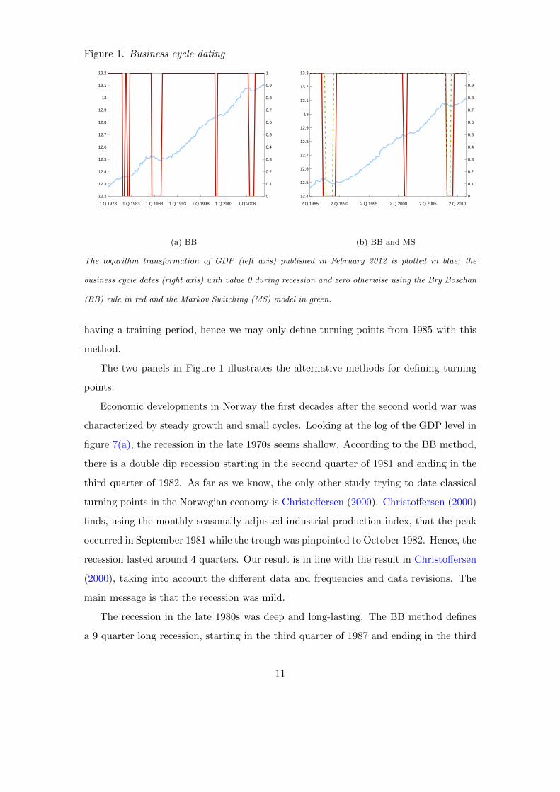
Figure 1. Business cycle dating

1.Q.1978 1.Q.1983 1.Q.1988 1.Q.1993 1.Q.1998 1.Q.2003 1.Q.2008

12.2

12.3

12.4

12.5

12.6

12.7

12.8

12.9

13

13.1

13.2

0

0.1

0.2

0.3

0.4

0.5

0.6

0.7

0.8

0.9

1

(a) BB

2.Q.1985 2.Q.1990 2.Q.1995 2.Q.2000 2.Q.2005 2.Q.2010

12.4

12.5

12.6

12.7

12.8

12.9

13

13.1

13.2

13.3

0

0.1

0.2

0.3

0.4

0.5

0.6

0.7

0.8

0.9

1

(b) BB and MS

The logarithm transformation of GDP (left axis) published in February 2012 is plotted in blue; the

business cycle dates (right axis) with value 0 during recession and zero otherwise using the Bry Boschan

(BB) rule in red and the Markov Switching (MS) model in green.

having a training period, hence we may only define turning points from 1985 with this

method.

The two panels in Figure 1 illustrates the alternative methods for defining turning

points.

Economic developments in Norway the first decades after the second world war was

characterized by steady growth and small cycles. Looking at the log of the GDP level in

figure 7(a), the recession in the late 1970s seems shallow. According to the BB method,

there is a double dip recession starting in the second quarter of 1981 and ending in the

third quarter of 1982. As far as we know, the only other study trying to date classical

turning points in the Norwegian economy is Christoffersen (2000). Christoffersen (2000)

finds, using the monthly seasonally adjusted industrial production index, that the peak

occurred in September 1981 while the trough was pinpointed to October 1982. Hence, the

recession lasted around 4 quarters. Our result is in line with the result in Christoffersen

(2000), taking into account the different data and frequencies and data revisions. The

main message is that the recession was mild.

The recession in the late 1980s was deep and long-lasting. The BB method defines

a 9 quarter long recession, starting in the third quarter of 1987 and ending in the third

11

quarter of 1989. Using the MS algorithm, see 7(b) in appendix, the recession starts in

the first quarter of 1988 and ends in the first quarter of 1989, i.e. lasting 5 quarters.

The characteristics of this period depend on the data vintage. In order to illustrate

the challenges associated with data revisions, we have calculated turning points using

national account vintages published in February 2010 and in February 2011, respectively.

See Figures 5 and 6 in the appendix. The recession in the late 1980s has become a double

dip recession according to the BB method and a triple dip recession when employing

the MS method. The whole recessionary period lasts longer for both methods. With

the 2010 and the 2011 vintages, the BB recession starts in the third quarter of 1987 and

does not end until the fourth quarter of 1991, a length of 18 quarters. The recession

defined by the Markov switching method starts in the fourth quarter of 1986 and ends

in the third quarter of 1991 (2010 vintage) or the first quarter of 1991 (2011 vintage).

To sum up, the timing of the recession in the late 1980s depends on which vintage we

use and on the choice of method.

Results using data published after Statistics Norway has changed their seasonally

adjustment of historical data favor the use of the BB method. The MS method produces

a recession that seems to start too late and to end too early, based on a judgemental

assessment of developments in the Norwegian economy in that period. It also seems

more reasonable when visually inspecting the log level of GDP.

We can compare the results from this period with findings in Christoffersen (2000).

He finds a peak in April 1989 and a trough in July 1990, ie around 5 quarters. Compared

with analyzing quarterly GDP, using monthly industrial production points to a shorter

recession, starting later and ending sooner. Again, this result seems unreasonable.

An alternative way of assessing how reasonable the turning points are, is to compare

their timing with developments in the unemployment rate, which has the advantage

of not being revised, see Figure 2. The unemployment rate starts to rise in the fourth

quarter of 1987, supporting the timing of a peak in 1987Q3 as defined by the BB method.

The next recession in the early 2000s is defined by the BB, while the MS method does

12

Figure 2. Unemployment rate and business cycle dating (BB) based on GDP

1.Q.1978 1.Q.1983 1.Q.1988 1.Q.1993 1.Q.1998 1.Q.2003 1.Q.2008

1

1.5

2

2.5

3

3.5

4

4.5

5

5.5

6

0

0.1

0.2

0.3

0.4

0.5

0.6

0.7

0.8

0.9

1

Unemployment rate (left axis) is plotted in blue; the business cycle dates (right axis) using BB and GDP

in red.

not pick any turning points in this period (but it peaks a short recession using 2010 and

2011 vintages). This mild recession is associated with the bursting of the “dot-com´´

bubble. The next big recession is, however, defined by all two methods. The MS method

defines a very short recession, 3 quarters starting with the third quarter of 2008. The

BB method defines the same peak in 2008Q2, but the trough does not occur until the

second quarter of 2009 - a recession lasting 5 quarters.

Judging the business cycles produced by the alternative methods, the BB method

seems to define turning points that are in line with the general assessment of develop-

ments in the Norwegian economy since the late 1970s. The MS defines peaks and troughs

in unlikely quarters or not at all.

4 Forecasting Norwegian turning points in real time

The turning points defined by the quarterly version of the Bry-Boschan method can

be interpreted as describing turning points in the “true” Norwegian classical business

cycles. One interesting question is then: Is it possible to predict the turning points in

real time?

13

In this exercise we will concentrate on the latest recession. The most important

reason for this choice is that prior to November 2011 revisions of seasonally adjusted

national affected data as far back as in the early 1980. Data vintages from the period

prior to November 2011 is increasingly different from the latest published vintage as

we move backwards in time. We would not expect, using real-time data, to be able

to predict turning points defined by the latest available vintages. This is also to some

extent true for the latest recession, since data are final only after three years of revisions.

However, these are revisions based on new information and we cannot avoid taking this

into account.

We will use the two methods described in section 2 on real-time data and compare

their ability to forecast turning points. The Markov switching techniques already com-

pute probabilities of being in one regime or the other (ie in recession or expansion).

The quarterly Bry-Boschan requires predictions to be able to define a turning point in

real time. We produce predictive densities from an autoregressive model AR(p) of order

p, where we fix p = 4 as in the Markov switching example.4 The median value of the

predictive densities is then used to extend the GDP level with the forecasts. The median

forecasts can be directly compared to define recession using the MS when regime 1 has

50% (or higher) probability. Since quarterly GDP is released with a lag of approximately

7 weeks, this means that if we add forecasts for 2 quarters to the latest available vintage

(ie a nowcast and a forecast), we may at the earliest predict a turning point 7 weeks

after it occurred. If we add a three-steps ahead forecast, it would in theory be possible

to forecast a turning point 5 weeks before it occurs. We will, however, confine ourselves

to predictive densities one- and two-steps ahead, as the uncertainty increases with the

horizon.

Both the BB and the MS can be augmented with leading indicators where a lead-

ing indicator is interpreted as a variable that timely summarizes the common cyclical

4Evaluations of point forecast accuracy are only relevant for highly restricted loss functions. More

generally, complete probability distributions over outcomes provide information helpful for making eco-

nomic decisions; see, for example, the discussions in Granger and Pesaran (2000), Timmermann (2006)

and Gneiting (2011).

14

movements of some coincident macroeconomic variables. We focus our analysis on two

classes of data: financial indices and survey data. Indicator models based on financial

data and survey data are likely candidates for being early in detecting turning points.

Publication are timely compared to GDP, and the nature of the statistics ensures that a

wide range of information and considerations are taken into account by financial market

participants, see Næs et al. (2011) and/or the respondents in the surveys, see Martinsen

et al. (2013). Note that financial data is high frequency and we choose the quarterly

version following Næs et al. (2011). All the surveys are just quarterly, as there are not

monthly surveys in Norway that have been published long enough to be useful in model

based forecasting. We have chosen two financial variables and three alternative surveys.

The financial indices are:

• Financial conditions index (FCI). The index is constructed using a dynamic fac-

tor model with financial variables, including interest rates, money and credit and

spreads.

• Amihud’s illiquidity ratio (Ill). The ratio is a measure of stock market liquidity,

see Amihud (2002)

The surveys are:

• The overall business confidence indicator from the business tendency survey for

manufactoring, mining and quarrying (BTS). The survey is conducted by Statistics

Norway in the last three weeks of the quarter and is published at the end of the

first month in the next quarter.

• The overall consumer confidence (CC) index (Indicator). The survey is conducted

by TNS Gallup in the fifth week of the quarter and is published in the middle of

the quarter.

• Expected growth in 6 months (all industries), from Norges Bank’s regional network

survey (RN). The survey is conducted in the first half of the quarter and published

around three weeks before the end of the quarter.

15

We use growth levels of all the five indicators together with GDP itself in bivariate

vector autoregressive models following Aastveit et al. (2013), and use the forecasts for

GDP to apply the BB rule.5 We also use the same variables as exogenous variables in

the augmented MS autoregressive models.6

4.1 Results

Results are presented in tables 1 to 4. From table 1, we can see that the five alternative

augmented BB models all predict in real time 2008Q3 as the peak quarter. The first

model to predict the downturn is the model with the consumer confidence indicator as the

second variable (in addition to GDP itself). When the survey is published 2 December,

using this to predict a two-step forecast (fourth quarter 2008 and first quarter 2009) for

GDP and then run the BB procedure on the resulting time series pinpoints a peak two

months after the quarter ended. All three survey models predict a peak in 2008Q3 as

soon as the survey for the fourth quarter of 2008 is published. The Markov switching

model augmented with the Norges Bank’s regional network survey also needs the fourth

quarter of 2008 to forecast the turning point, but starting in 2007Q4, which seems too

early for Norway. The other models predict the turning point later and three of them

starting in 2008Q2.

Table 2 summarizes the peaks identified in the previous section using ex post data,

more precisely the vintage published in February 2012. In real time, the forecasted

peaks occur later than the peaks defined ex post using the full database. This is no

surprise, since ex post data contains information from four more years. Furthermore,

data is substantially revised. For example, in Figure 3, we compare the log levels of

GDP vintages published in November 2008 and February 2012, respectively. In the 2008

5Applying univariate autoregressive models for the GDP extended with exogenous variables produces

less accurate results than bivariate VARs, confirming evidence in Aastveit et al. (2013).6We also investigated two definitions of unemployment; the unemployment rate from the Labor Force

Survey and the registered unemployment rate; and the use of the levels; but results in all these cases are

inferior with recessions starting too late and lasting too long.

16

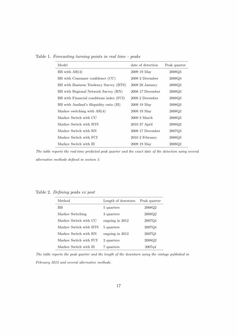
Table 1. Forecasting turning points in real time - peaks

Model date of detection Peak quarter

BB with AR(4) 2009 19 May 2008Q3

BB with Consumer confidence (CC) 2008 2 December 2008Q3

BB with Business Tendency Survey (BTS) 2009 28 January 2008Q3

BB with Regional Network Survey (RN) 2008 17 December 2008Q3

BB with Financial conditions index (FCI) 2008 2 December 2008Q3

BB with Amihud’s illiquidity ratio (Ill) 2009 19 May 2008Q3

Markov switching with AR(4) 2009 19 May 2008Q2

Markov Switch with CC 2009 3 March 2008Q3

Markov Switch with BTS 2010 27 April 2008Q2

Markov Switch with RN 2008 17 December 2007Q3

Markov Switch with FCI 2010 2 February 2008Q3

Markov Switch with Ill 2009 19 May 2008Q2

The table reports the real-time predicted peak quarter and the exact date of the detection using several

alternative methods defined in section 2.

Table 2. Defining peaks ex post

Method Length of downturn Peak quarter

BB 5 quarters 2008Q2

Markov Switching 3 quarters 2008Q2

Markov Switch with CC ongoing in 2012 2007Q4

Markov Switch with BTS 5 quarters 2007Q4

Markov Switch with RN ongoing in 2012 2007Q1

Markov Switch with FCI 2 quarters 2008Q2

Markov Switch with Ill 7 quarters 2007q4

The table reports the peak quarter and the length of the downturn using the vintage published in

February 2012 and several alternative methods.

17

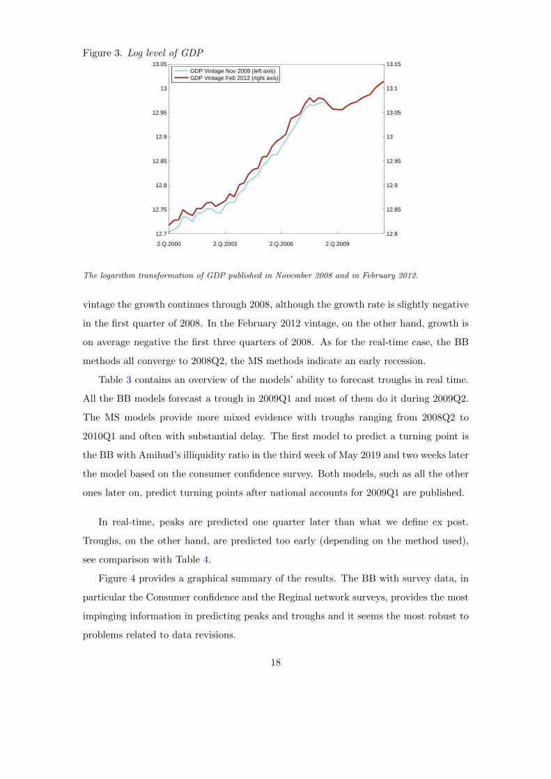
Figure 3. Log level of GDP

2.Q.2000 2.Q.2003 2.Q.2006 2.Q.2009

12.7

12.75

12.8

12.85

12.9

12.95

13

13.05

12.8

12.85

12.9

12.95

13

13.05

13.1

13.15

GDP Vintage Nov 2008 (left axis)GDP Vintage Feb 2012 (right axis)

The logarithm transformation of GDP published in November 2008 and in February 2012.

vintage the growth continues through 2008, although the growth rate is slightly negative

in the first quarter of 2008. In the February 2012 vintage, on the other hand, growth is

on average negative the first three quarters of 2008. As for the real-time case, the BB

methods all converge to 2008Q2, the MS methods indicate an early recession.

Table 3 contains an overview of the models’ ability to forecast troughs in real time.

All the BB models forecast a trough in 2009Q1 and most of them do it during 2009Q2.

The MS models provide more mixed evidence with troughs ranging from 2008Q2 to

2010Q1 and often with substantial delay. The first model to predict a turning point is

the BB with Amihud’s illiquidity ratio in the third week of May 2019 and two weeks later

the model based on the consumer confidence survey. Both models, such as all the other

ones later on, predict turning points after national accounts for 2009Q1 are published.

In real-time, peaks are predicted one quarter later than what we define ex post.

Troughs, on the other hand, are predicted too early (depending on the method used),

see comparison with Table 4.

Figure 4 provides a graphical summary of the results. The BB with survey data, in

particular the Consumer confidence and the Reginal network surveys, provides the most

impinging information in predicting peaks and troughs and it seems the most robust to

problems related to data revisions.

18

Table 3. Forecasting turning points in real time - troughs

Model date of detection Trough quarter

BB with AR(4) 2009 19 May 2009Q1

BB with Consumer confidence (CC) 2009 2 June 2009Q1

BB with Business Tendency Survey (BTS) 2009 28 July 2009Q1

BB with Regional Network Survey (RN) 2009 10 June 2009Q1

BB with Financial conditions index (FCI) 2009 2 July 2009Q1

BB with Amihud’s illiquidity ratio (Ill) 2009 19 May 2009Q1

Markov switching with AR(4) 2009 19 May 2009Q1

Markov Switch with CC 2010 7 December 2010Q1

Markov Switch with BTS 2010 27 April 2009Q1

Markov Switch with RN 2008 17 December 2008Q2

Markov Switch with FCI 2010 2 February 2008Q4

Markov Switch with Ill 2009 19 August 2009Q1

The table reports the real-time predicted though quarter and the exact date of the detection using several

methods.

Table 4. Defining troughs ex post

Method Length of downturn Trough quarter

BB 5 quarters 2009Q3

Markov Switching 3 quarters 2009Q1

Markov Switch with CC ongoing in 2012 ..

Markov Switch with BTS 5 quarters 2009Q1

Markov Switch with RN ongoing in 2012 ..

Markov Switch with FCI 2 quarters 2008Q4

Markov Switch with Ill 7 quarters 2009q3

The table reports the though quarter and the length of the downturn using the vintage published in

February 2012 and several alternative methods.

19

Figure 4. Turning point forecasts

1 2 3 4 1 2 3 4 1 2 3 4 1 2 3 4 1 2 3 4BryBorschan with AR4

Ex postRT inRT out

BryBorschan with Consumer ConfidenceEx postRT inRT out

BryBorschan with Business tendency surveyEx postRT inRT out

BryBorschan with Regional network surveyEx postRT inRT out

BryBorschan with Financial conditions index (FCI)Ex postRT inRT out

BryBorschan with Amihud's illiquidity index (Ill)Ex postRT inRT out

Markov Switcing with AR4 Ex postRT inRT out

Markov Switcing with with Consumer ConfidenceEx postRT inRT out

Markov Switcing with Business tendency surveyEx postRT inRT out

Markov Switcing with Regional network surveyEx postRT inRT out

Markov Switcing with Financial conditions index (FCI)Ex postRT inRT out

Markov Switcing with Amihud's illiquidity index (Ill)Ex postRT inRT out

2007 2008 2009 2010 2011

For each class of models, the figure illustrates the length of the recession in lines “Ex-post” using ex-post

data. Red denotes quarters where the economy is in recession. The lines denoted “RT” in show which

quarter is the first in the recession in real time, i.e the peak quarter is the quarter before the quarter

marked in red. In the lines denoted “RT out”, the red quarter is the trough quarter in real time. Black

vertical lines with the real-time data indicate which date the turning point was detected.

20

5 Conclusion

We compare several methods to define and forecast in real time classical business cycle

turning points in Norway, a country which does not have an official business cycle indi-

cator. We apply the Bry and Boschan rule (BB), an autoregressive Markov Switching

model (MS), and the two methodologies augmented with financial indicators and sur-

vey data, using several vintages of Norwegian Gross Domestic Product as the business

cycle indicator. We find that the BB provides the most reliable definition of business

cycles using different vintages and when augmented with density forecasts from survey

models provides more timely predictions for Norwegian turning points than the Markov

Switching models both using final vintage and, above all, real-time data.

Our analysis focuses on a single country and just one, large, recession. We think,

however, the analysis provides useful indications on how to construct classical business

cycle turning points using timely information.

References

Aastveit, K., K. Gerdrup, A. Jore, and L. Thorsrud (2013). Nowcasting gdp in real-time:

A density combination approach. Journal of Business Economics and Statistics forth-

coming.

Aastveit, K. and T. Trovik (2012). Nowcasting norwegian gdp: the role of asset prices

in a small open economy. Empirical Economics 42 (1), 95–119.

Abberger, K. (2007). Qualitative business surveys and the assessment of employment –

a case study for Germany. International Journal of Forecasting 23 (2), 249–258.

Amihud, Y. (2002). Illiquidity and stock returns: Cross-section and time-series effects.

Journal of Financial Markets 5, 31–56.

Anas, J., M. Billio, L. Ferrara, and G. L. Mazzi (2008). A System for Dating and

Detecting Turning Points in the Euro Area. The Manchester School 76, 549–577.

21

Ang, A., G. Bekaert, and M. Wei (2007, May). Do macro variables, asset markets, or

surveys forecast inflation better? Journal of Monetary Economics 54 (4), 1163–1212.

Billio, M., R. Casarin, F. Ravazzolo, and H. van Dijk (2012). Combination schemes

for turning point predictions. Quarterly Review of Economics and Finance 52 (4),

402–412.

Bjørnland, H. C. (1995). Trends, cycles, and measures of persistence in the Norwegian

economy. Statistics Norway.

Bry, G. and C. Boschan (1971). Cyclical Analysis of Time Series: Selected Procedures

and Computer Programs. NBER Technical Paper 20.

Burns, A. and W. Mitchell (1948). Measuring business cycles. NBER.

Chauvet, M. (1998). An econometric characterization of business cycle dynamics with

factor structure and regime switching. International Economic Review 39 (4), 969–996.

Christoffersen, P. (2000). Dating the turning points of nordic business cycles. EPRU

Working paper No. 00/13 .

Claveria, O., E. Pons, and R. Ramos (2007). Business and consumer expectations and

macroeconomic forecasts. International Journal of Forecasting 23 (1), 47–69.

Clements, M. P. and H. M. Krolzig (1998). A comparison of the forecast performances

of Markov-switching and threshold autoregressive models of US GNP. Econometrics

Journal 1, C47–C75.

Cochrane, J. and M. Piazzesi (2005). Bond risk premia. American Economic Review 94,

138–160.

Diebolt, J. and C. P. Robert (1994). Estimation of finite mixture distributions through

Bayesian sampling. Journal of the Royal Statistical Society B 56, 363–375.

Eika, T. and K.-G. Lindquist (1997). Konjunkturimpulser fra utlandet. Statistics Norway.

22

Fama, E. F. and M. R. Gibbons (1984). A comparison of inflation forecasts. Journal of

Monetary Economics 13 (3), 327–348.

Fruhwirth-Schnatter, S. (2006). Mixture and Markov-swithing Models. New York:

Springer.

Gneiting, T. (2011). Making and evaluating point forecasts. Journal of the American

Statistical Association 106, 746–762.

Goldfeld, S. M. and R. E. Quandt (1973). A Markov Model for Switching Regression.

Journal of Econometrics 1, 3–16.

Granger, C. and M. Pesaran (2000). Economic and statistical measures of forecast

accuracy. Journal of Forecasting 19, 537–560.

Guidolin, M. (2011). Markov switching models in empirical finance. Advances in Econo-

metrics 27, 1–86.

Hamilton, J. D. (1989). A new approach to the economic analysis of nonstationary time

series and the business cycle. Econometrica 57, 357–384.

Hamilton, J. D. (2011). Calling recessions in real time. International Journal of Fore-

casting 27(4), 1006–1026.

Hansson, J., P. Jansson, and M. Lof (2005). Business survey data: Do they help in

forecasting GDP growth? International Journal of Forecasting 21, 377–389.

Harding, D. and A. Pagan (2002). Dissecting the Cycle: A Methodological Investigation.

Journal of Monetary Economics 49, 365–381.

Harvey, C. (1989). The real term structure and consumption growth. Journal of Finan-

cial Economics 22, 305–333.

Jochmann, M., G. Koop, and R. Strachan (2010). Bayesian forecasting using stochas-

tic search variable selection in a VAR subject to breaks. International Journal of

Forecasting 26(2), 326–347.

23

Kim, C. J. and C. J. Murray (2002). Permanent and Transitory Components of Reces-

sions. Empirical Economics 27, 163–183.

Kim, C. J. and J. Piger (2000). Common stochastic trends, common cycles, and asymme-

try in economic fluctuations. Working paper, n. 681, International Finance Division,

Federal Reserve Board, Semptember 2000.

Krolzig, H.-M. (1997). Markov Switching Vector Autoregressions. Modelling, Statistical

Inference and Application to Business Cycle Analysis. Berlin: Springer.

Krolzig, H.-M. (2000). Predicting Markov-Switching Vector Autoregressive Processes.

Nuffield College Economics Working Papers, 2000-WP31.

Ludvigson, S. and S. Ng (2009). Macro factors in bond risk premia. Review of Financial

Studies 22, 5027–5067.

Lui, S., J. Mitchell, and M. Weale (2010a). Qualitative business surveys: signal or noise?

Journal of the Royal Statistical Society: Series A Forthcoming.

Lui, S., J. Mitchell, and M. Weale (2010b). The utility of expectational data: Firm-level

evidence using matched qualitative-quantitative UK surveys. International Journal of

Forecasting Forthcoming.

Martinsen, K., F. Ravazzolo, and F. Wulfsberg (2013). Forecasting macroeconomic

variables using disaggregate survey data. International Journal of Forecasting forth-

coming.

Mehra, Y. P. (2002). Survey measures of expected inflation: revisiting the issues of

predictive content and rationality. Economic Quarterly (Sum), 17–36.

Næs, R., J. Skjeltorp, and B. Ødegaard (2011). Stock market liquidity and the business

cycle. Journal of Finance, 2011, 66, 139-176. 66, 139–176.

Orphanides, A. and S. van Norden (2002). The unreliability of output-gap estimates in

real time. The Review of Economics and Statistics 84 (4), 569–583.

24

Schumpeter, J. A. (1954). History of Economic Analysis. London: George Allen and

Unwin.

Tanner, M. and W. Wong (1987). The calculation of posterior distributions by data

augmentation. Journal of the American Statistical Association 82, 528–550.

Thomas, L. B. (1999). Survey measures of expected U.S. inflation. Journal of Economic

Perspectives 13 (4), 125–144.

Timmermann, A. (2006). Forecast combinations. In G. Elliott, C. W. J. Granger, and

A. Timmermann (Eds.), Handbook of Economic Forecasting, Volume 1, pp. 136–96.

Amsterdam: Elsevier.

Vermaak, J., C. Andrieu, A. Doucet, and S. J. Godsil (2004). Reversible jump Markov

chain Monte Carlo strategies for Bayesian model selection in autoregressive processes.

Journal of Time Series Analysis 25, 785–809.

25

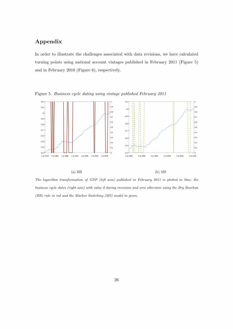
Appendix

In order to illustrate the challenges associated with data revisions, we have calculated

turning points using national account vintages published in February 2011 (Figure 5)

and in February 2010 (Figure 6), respectively.

Figure 5. Business cycle dating using vintage published February 2011

1.Q.1978 1.Q.1983 1.Q.1988 1.Q.1993 1.Q.1998 1.Q.2003 1.Q.2008

12.3

12.4

12.5

12.6

12.7

12.8

12.9

13

13.1

13.2

0

0.1

0.2

0.3

0.4

0.5

0.6

0.7

0.8

0.9

1

(a) BB

2.Q.1985 2.Q.1990 2.Q.1995 2.Q.2000 2.Q.2005 2.Q.2010

12.4

12.5

12.6

12.7

12.8

12.9

13

13.1

0

0.1

0.2

0.3

0.4

0.5

0.6

0.7

0.8

0.9

1

(b) MS

The logarithm transformation of GDP (left axis) published in February 2011 is plotted in blue; the

business cycle dates (right axis) with value 0 during recession and zero otherwise using the Bry Boschan

(BB) rule in red and the Markov Switching (MS) model in green.

26

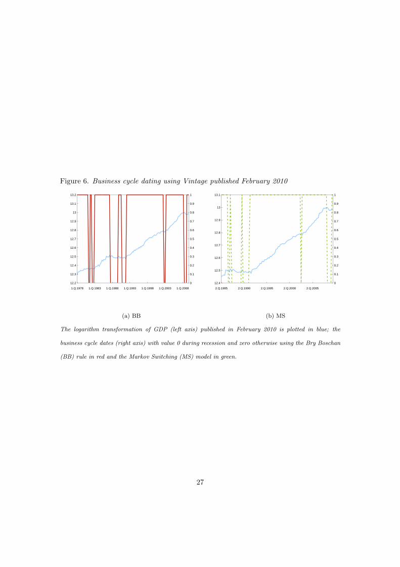
Figure 6. Business cycle dating using Vintage published February 2010

1.Q.1978 1.Q.1983 1.Q.1988 1.Q.1993 1.Q.1998 1.Q.2003 1.Q.2008

12.2

12.3

12.4

12.5

12.6

12.7

12.8

12.9

13

13.1

13.2

0

0.1

0.2

0.3

0.4

0.5

0.6

0.7

0.8

0.9

1

(a) BB

2.Q.1985 2.Q.1990 2.Q.1995 2.Q.2000 2.Q.2005

12.4

12.5

12.6

12.7

12.8

12.9

13

13.1

0

0.1

0.2

0.3

0.4

0.5

0.6

0.7

0.8

0.9

1

(b) MS

The logarithm transformation of GDP (left axis) published in February 2010 is plotted in blue; the

business cycle dates (right axis) with value 0 during recession and zero otherwise using the Bry Boschan

(BB) rule in red and the Markov Switching (MS) model in green.

27