FORECASTING OFFICE BUILDING RENTAL GROWTH USING A … · 2018-07-23 · different at six different points in the property market cycle. In a defining study, Pyhrr, Roulac and Born

Pacific Rim Property Research Journal, Vol 10, No 3 283

FORECASTING OFFICE BUILDING RENTAL GROWTH USING A DYNAMIC APPROACH

MARCELLO TONELLI, MERVYN COWLEY

and

TERRY BOYD

Queensland University of Technology ABSTRACT Numerous econometric models have been proposed for forecasting property market performance, but limited success has been achieved in finding a reliable and consistent model to predict property market movements over a five to ten year timeframe. This research focuses on office rental growth forecasts and overviews many of the office rent models that have evolved over the past 20 years. A model by DiPasquale and Wheaton is selected for testing in the Brisbane office market. The adaptation of this model did not provide explanatory variables that could assist in developing a reliable, predictive model of office rental growth. In light of this result, this paper suggests a system dynamics framework that includes an econometric model based on historical data as well as user input guidance for the primary variables. The rent forecast outputs would be assessed having regard to market expectations and probability profiling undertaken for use in simulation exercises. Keywords: Forecasting, office rents, system dynamics, econometric modelling,

simulation. INTRODUCTION Earlier approaches in estimating rental growth rates in discounted cash flow valuation exercises were often overly simplistic, generating projections that were far from realistic (Hendershott, 1996; Born & Pyhrr, 1994). Kummerow (1997) found, during the 1980s, that Australian valuers commonly adopted a single, linear and compounding rent growth rate in their assessments. A recent survey of valuers in Brisbane, Australia (Cowley, 2003) found that most valuers use broad cyclical rent forecasts in cash flow studies, but that the conservative nature of recent forecasts in this city appear to lack a methodology and fortitude in recognising the volatility of the property market. Figure 1 illustrates this inconsistency with a

284 Pacific Rim Property Research Journal, Vol 10, No 3

comparison of the historical volatility of prime office rents spliced onto the median of forecasts from five major valuation firms. In this case, the forecasts were relatively close, ranging between zero and five percent growth per annum. The standard deviations of the five forecasts ranged between 0.4% and 1.9%, while the historical volatility was 14.4%. Figure 1: Historical and forecast percentage change – Brisbane prime office rents

-15.0%

-10.0%

-5.0%

0.0%

5.0%

10.0%

15.0%

20.0%

25.0%

30.0%

35.0%

1971

1974

1977

1980

1983

1986

1989

1992

1995

1998

2001

2004

2007

2010

Year

% C

hang

e

Actual Historical Change 5 Valuation

Firms' Median Forecast

Source: BIS Shrapnel & CBD Valuation Firms Asset managers are emphasizing the importance of realistic rental growth forecasts and requiring valuers to justify their forecasts. This study examines whether existing or adapted econometric models developed from historical data can be used to predict future rental growth rates. Initially a literature review of property cycle analysis is undertaken and thereafter an econometric model is tested using data from the Brisbane office market. As the results from this study are unhelpful in providing a model for predictive purposes, reference is made to the incorporation of the simulation process and the incorporation of System Dynamics in the forecasting process. LITERATURE REVIEW ON PROPERTY CYCLES Much research has been devoted to the nature and causes of property market cycles. Born and Pyhrr (1994) conducted practical tests to determine the impacts of


accounting for market and economic cycles in property cash flow assessments. McGough and Tsolacos (1995) examined commercial building activity in the UK and its procyclicality with demand side factors, such as GDP and employment growth. Clayton (1996) found, in a Canadian study, real estate returns were a function of general capital market conditions. Kaiser (1997) investigated real estate cycles over a long term extending from the 1800s and argued for the existence of “long cycles” with durations of 50 to 60 years. These “long cycles” were said to be driven by prior periods of above-average inflation. Canter, Gordon and Mosburgh (1997) examined the impact of economic fundamentals on building vacancy rates as a generator of property cycles. The relationship between macroeconomic variables and the property market was said to provide the ability to distinguish between the different stages of real estate cycles when looking at property returns (Grissom and DeLisle, 1999). Mueller (1999) determined rental growth rates to be statistically different at six different points in the property market cycle. In a defining study, Pyhrr, Roulac and Born (1999) nominated cycles’ “pervasive and dynamic impacts on real estate returns, risks and investment values”. Again, this study raised the key linkages between macroeconomic factors and property supply and demand factors. With a wider view, Dehesh and Pugh (2000) considered the impact of globalisation, economic agglomeration and financial deregulation on real estate cycles. Many researchers have recognised the cyclical influences and negative impacts of overbuilding on office vacancy rates and, consequently, on office rents. Barras (1994) considered several cyclical influences of different periodicity conspired to produce major, speculative building booms. Barras also considered these occurrences to be self-replicating over time. Gallagher and Wood (1999) noted the property market’s tendency to over-react to economic trends, generating excess office construction and this was known to have a negative impact on market performance. The causes of these occurrences were quoted as being the long-term investment nature of real estate; development lags; space demand uncertainty; high adjustment (acquisition / disposal) costs; and the “unbridled enthusiasm” of developers. In this context, Kummerow (1999) spoke of “allocative and production inefficiencies” in terms of resources. Sivitanidou and Sivitanides (2000) raised the concept of “irreversible investment” in relation to the “highly cyclical and highly volatile” office-commercial construction activity in the US. Past research on property cycles and the supply and demand dynamics of property markets has been paralleled by studies aimed at developing rent, return and space supply forecasting models. Office rent models have been evolving over the past twenty years and the majority of the models explicitly quantify causal relationships between changes in rent levels and property market and macroeconomic determinants. Figure 2 provides a visual representation of the 22 identified models.


Figure 2:

Of interest is a comparison of the relative dominance of the explanatory variables adopted in the 22 models. The following table provides a representation of the relative level of adoption of the various property, market, economic and financial factors.

Table 1: Office rent explanatory variables adopted by researchers Office Rent Models – Determinants Property Market Factors Economic / Financial Factors

Researcher(s) Year

Rent

Equilibrium

Rent

Vacancy R

ate

Natural

Vacancy R

ate

Building

Characteristics

Space A

bsorption

Space Supply

Occupied Space

Location

Construction

Costs

Lease Aspects

House Prices

Operating C

osts

Market

Conditions

Economic

Activity

Economic

Uncertaint y

Interest Rates

Employm

ent

Unem

ployment

Stock Market

Inflation

Taxation

Rosen KT 1984 Hekman JS 1985 Shilling J, Sirman C & Corgel J 1987 Wheaton WC & Torto RG 1988 Frew J & Jud GD 1988 Gardiner C & Henneberry J 1988 Gardiner C & Henneberry J 1991 Dobson SM & Goddard JA 1992 Glascock JL, Kim M & Sirmans CF 1993 Giussani B, Hsia M & Tsolacos S 1993 Hendershott PH et al* 1996 DiPasquale D & Wheaton WC 1996 Hendershott PH 1997 Dunse N & Jones C 1998 D’Arcy E et al 1999 Hendershott PH et al 1999 Wheaton WC 1999 Chaplin R 2000 Murray J 2000 MacFarlane J et al 2002 Hendershott PH et al 2002 Tse RYC & Fischer D 2003

Observations 11 4 13 7 3 1 8 2 2 4 0 1 3 2 6 1 5 6 1 0 1 1

Pacific Rim

Property Research Journal, V

ol 10, No. 3

287


Figure 3 displays the relative dominance of the explanatory variables adopted by the researchers. Figure 3: Explanatory variables – frequency of adoption by researchers

0 5 10 15

Observed Rent

Vacancy Rate

Building Characteristics

Space Supply

Location

Lease Aspects

Operating Costs

Economic Activity

Interest Rates

Unemployment

Inflation

Det

erm

inan

ts

Observations

Economic / Fianancial Factors

Propert y Market Factors

Aside from historical or observed rents, the dominant property / market determinants adopted for office rents include observed and natural vacancy rates and space supply. The prevalent economic / financial determinants adopted include economic activity, interest rates and employment. Dominant econometric models McDonald (2002) surveyed office market econometric models and the study focused on the models developed by Wheaton, Torto and Evans (1997) and Hendershott, Lizieri and Matysiak (1999). Both these models were estimated for the London office market and served as forerunners to the “RICS model” developed in 2000 by the RICS Research Foundation. In commenting on the Wheaton Torto and Evans model, McDonald stated that its “theoretical framework is arguably the best among available models”. A varied version of this model was estimated for the San Francisco office market (DiPasquale and Wheaton, 1996). A diagrammatic representation of the workings of this model has been produced in Figure 4.


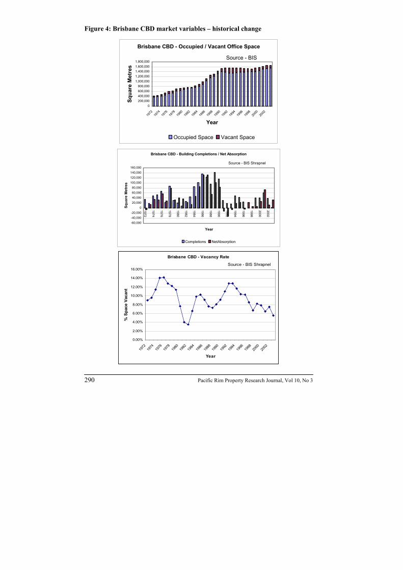
Figure 4: Conceptual map – derived from DiPasquale and Wheaton office market model (1996) The publication of full econometric models is relatively rare. The DiPasquale / Wheaton – Wheaton / Torto / Evans models incorporate the majority of the explanatory variables found to be dominant in the many models that have evolved over time. This together with McDonald’s (2002) support for the framework and the relative transparency of how the models were applied to the San Francisco and London markets assisted in selecting the framework for testing and forecasting with data for Brisbane, Australia. The MacFarlane et al. (2002) test of a modified version of the “RICS model” using Sydney market data demonstrated the difficulties of applying a model with the assumption of universality across other international office markets. However, as a starting point, this study is limited to a direct application of the DiPasquale / Wheaton model without regard to potential differences between Brisbane and San Francisco in market dynamics. Brisbane Central Business District data Brisbane is the capital of Queensland and is the third largest Australian central business district in terms of office floor area with a total net lettable area of approximately 1.65M square metres. Some of the city’s fundamental office market variables and their change over the last 31 years are shown in Figure 4.

Desired Rent

Vacancy

Desired Occ. Space

Employment

Net Absorption

Desired Completions

Completions

Deman

Lag TimeStock

Demolitions

Lag Time

Occupied Space

Rent

Lag Time

Lag Time

STRONG RELATIONSHIPS

WEAK RELATIONSHIPS

LAGS

EXOGENOUS VARIABLES


Figure 4: Brisbane CBD market variables – historical change

Brisbane CBD - Occupied / Vacant Office Space

0200,000400,000600,000800,000

1,000,0001,200,0001,400,0001,600,0001,800,000

1972

1974

1976

1978

1980

1982

1984

1986

1988

1990

1992

1994

1996

1998

2000

2002

YearSq

uare

Met

res

Occupied Space Vacant Space

Source - BIS

Brisbane CBD - Building Completions / Net Absorption

-60,000-40,000-20,000

020,00040,00060,00080,000

100,000120,000140,000160,000

1972

1974

1976

1978

1980

1982

1984

1986

1988

1990

1992

1994

1996

1998

2000

2002

Year

Squa

re M

etre

s

Completions NetAbsorption

Source - BIS Shrapnel

Brisbane CBD - Vacancy Rate

0.00%

2.00%

4.00%

6.00%

8.00%

10.00%

12.00%

14.00%

16.00%

1972

1974

1976

1978

1980

1982

1984

1986

1988

1990

1992

1994

1996

1998

2000

2002

Year

% S

pace

Vac

ant



Brisbane CBD - Prime Face / Effective Rent (89-90$)

$0

$50

$100

$150

$200

$250

$300

$350

$400

$450

$500

1972

1974

1976

1978

1980

1982

1984

1986

1988

1990

1992

1994

1996

1998

2000

2002

Year

Rate

/ m

2Prime Face Rent Prime Effective Rent


A frequent lament of property researchers is the quality and extent of available property market data (eg: Jones, 1995; Mitchell and McNamara, 1997; Tsolacos and McGough, 1999; Mueller, 2002; MacFarlane, Murray, Parker and Peng, 2002). In this instance, due to the lack of longer term CBD employment data, the scope of the study has been limited to annual data extending from 1980 to 2003. Some summary statistics for the data utilized for model testing are given in Table 2. Table 2: Data summary statistics

Variable Period Mean Std Dev Minimum Maximum

Vacancy (%) 1980-2003 8.5% 2.4% 3.5% 12.9%

Occupied Space (∆m²) 1980-2003 37,450m² 43,636m² -33,600m² 132,100m²

Net Absorption (∆m²) 1980-2003 37,433m² 43,646m² -33,600m² 132,000m²

Employment (∆) 1981-2003 1,450 1,689 -1,300 4,100

Withdrawals (m²) 1980-2003 14,825m² 13,698m² 0m² 48,300m²

Completions (m²) 1980-2003 52,979m² 43,992m² 0m² 142,300m²

Work Space Ratio (∆m²) 1981-2003 0.2m² 0.8m² -1.0m² 2.3m²

Gross Effective Rent ($/m²) 1980-2003 $195 $39 $152 $264

Results of Brisbane study A summary of some of the results from applying the DiPasquale and Wheaton model to the Brisbane data is given in the following sections. Some adjustments to the lag periods have been adopted to better reflect the workings of the Brisbane market.


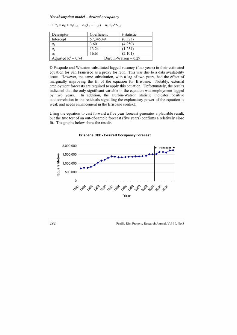
Net absorption model – desired occupancy OC*t = α0 + α1Et-2 + α2(Et – Et-2) + α3Et-2*Vt-2

Descriptor Coefficient t-statistic Intercept 57,345.49 (0.323) α1 3.60 (4.250) α2 13.24 (1.254) α3 16.61 (2.101) Adjusted R2 = 0.74 Durbin-Watson = 0.29

DiPasquale and Wheaton substituted lagged vacancy (four years) in their estimated equation for San Francisco as a proxy for rent. This was due to a data availability issue. However, the same substitution, with a lag of two years, had the effect of marginally improving the fit of the equation for Brisbane. Notably, external employment forecasts are required to apply this equation. Unfortunately, the results indicated that the only significant variable in the equation was employment lagged by two years. In addition, the Durbin-Watson statistic indicates positive autocorrelation in the residuals signalling the explanatory power of the equation is weak and needs enhancement in the Brisbane context. Using the equation to cast forward a five year forecast generates a plausible result, but the true test of an out-of-sample forecast (five years) confirms a relatively close fit. The graphs below show the results.

Brisbane CBD - Desired Occupancy Forecast

0

500,000

1,000,000

1,500,000

2,000,000

1982

1984

1986

1988

1990

1992

1994

1996

1998

2000

2002

2004

2006

2008

Year

Squa

re M

etre

s

F o recast


However, calculation of the Theil’s U-statistic (1.05) for the out-of-sample forecast infers a naïve forecast would marginally eclipse the forecast derived from the equation in terms of accuracy. Equilibrium rent R* = µ0 – µ1Vt-1 + µ2 ABt-1 St-1

Descriptor Coefficient t-statistic Intercept 160.27 (7.116) µ1 103.26 (0.436) µ2 825.28 (5.220) Adjusted R2 = 0.53 Durbin-Watson = 1.18

Surprisingly, the vacancy rate variable did not register as significant in this case, while the lagged absorption / stock ratio was found to influence the level of equilibrium rent. The equation is not a good fit (adjusted R² of 0.53) and a case for further refinement of the equation’s structure is supported by a degree of positive autocorrelation remaining in the residuals. Using the stock, new supply, absorption and vacancy forecasts derived from the model, a five year forecast of the equilibrium rent was generated. Applying the results to the DiPasquale and Wheaton rent equation [Rt = µ3(R* - Rt-1) + Rt-1 where µ3 is an adjustment parameter quantifying speed of movement towards equilibrium rent], a five year median gross effective rent forecast is generated. The results were

Brisbane CBD - Desired Occupancy Forecast

0200,000400,000600,000800,000

1,000,0001,200,0001,400,0001,600,0001,800,000

1981 1983 1985 1987 1989 1991 1993 1995 1997 1999 2001 2003

Year

Squa

re M

etre

s

Actual Forecast


found to be quite erratic and the out-of-sample forecast Theil’s U-statistic (2.76) confirmed a naïve forecast would produce a far superior result.

Brisbane CBD - Median Gross Effective Rent Forecast

$0.0

$50.0

$100.0

$150.0

$200.0

$250.0

$300.0

1980

1982

1984

1986

1988

1990

1992

1994

1996

1998

2000

2002

2004

2006

2008

Year

Rat

e / m

2

Forecast

Brisbane CBD - Mean Rent - Out-of-Sample Forecast

$0

$50

$100

$150

$200

$250

$300

1980

1981

1982

1983

1984

1985

1986

1987

1988

1989

1990

1991

1992

1993

1994

1995

1996

1997

1998

1999

2000

2001

2002

2003

Year

$/m

2

Actual Forecast

The results of this analysis are disappointing although no reasonable fit was anticipated due the differences between the markets. While further work is required to estimate a model that exhibits a sound fit to the Brisbane market, this research will extend beyond the application of econometric models into a potentially complementary area of system dynamics.


SYSTEM DYNAMICS System dynamics theories offer the opportunity to model the complex interrelationships of the real estate environment and to observe their dynamic behaviour over time, with particular respect to how these interrelationships impact the investment prospects facing the building company or even the private investor. Simulation modelling in general seems to be a relatively new concept in the real estate industry. Other industry sectors have proven that the use of well-calibrated structural models, such as system dynamics simulators, can do a reasonable job of forecasting in situations where regression and trend forecasts have proven their individual weaknesses (Sterman, 1988; Sterman, 2000; Lyneis, 2000), but the use of such theories in real estate markets has been very sporadic. Forrester (1969), founder of system dynamics, developed Urban Dynamics, a complex model counting 150 equations for the prediction of urban growth and decline, used to understand America’s urban crisis. Vennix (1996) offers a case study to illustrate the dynamics of the housing market from the perspective of housing associations. Kim and Lannon (1991) examined Minneapolis’ real estate activity arguing that delays, self-ordering dynamics, speculation and short-term individual gain are the factors that need to be addressed. Kummorow (1997, 1999) developed a series of dynamic models, integrating econometric and simulation principles with forecasting methods, to study and forecast supply and demand cycles for the areas of Sydney and Perth. Aptek Associates LLC also developed a series of corporate real estate simulation tools that can be used to do more accurate planning and forecasting (Klammt, 2001). Bakken & Sterman (1993) designed a real estate flight simulator, in which the user takes command of a firm in the volatile market of office buildings and pilots it from start-up to success. The adaptation of a statistical model to a system dynamics framework has several advantages. First of all, spreadsheet analyses are static in nature, no matter how complex the macros are, and do not take into account the changing dynamics of the market environment. Conversely, a system dynamics model does not simply determine future rates under current market conditions, but it also considers changes that occur overtime from the interaction of different variables. Secondly, allowing parameters such as employment growth and demolition rate to be varied exogenously by the user adds credibility to the simulation model, because it gives the user a better understanding of the industry structure and makes the user participate to the decision making process. On the other hand, we must also be very careful with the type and amount of freedom granted to the user. Assumptions should not deviate from reasonable ranges set in consistency with historical patterns to prevent the model from coming up with illogical values. Additionally, only a limited number of parameters should be given the possibility


of having arbitrary values: the main inputs such as supply and demand should always be kept endogenous to the system. Bertsche, Crawford and Macadam (1996) assert the existence of a deep body of theoretical literature that praise the power of simulations to change behaviour by giving managers the opportunity to experiment, test their assumptions, and learn from their mistakes in a risk-free environment. But the literature has little to say about how the theory can be applied in real corporate situations. In fact, their study also shows that over 60 percent of US corporations have used some sort of simulation and that only a few have succeeded. This statistic shows that simulations can play a useful role in successful transformations, but if they are poorly designed they have no more than an entertainment value. For this reason, the econometric structure of the model remains a primary concern and it needs to be designed on the basis of logic, expert opinion and historical trends. Application of system dynamics Due to the inadequacy of existing econometric models, this study is considering whether a system dynamics approach can provide a basis for rental growth forecasts. A four-step approach has been identified:

i. collect all the available mental and written information ii. develop the structure of the model iii. simulate and compare outputs with historical data iv. evaluate the discrepancies.

a) The first step is to collect information from many different sources:

professional experience and knowledge, written database and numerical database. Mental and written information will then be used to structure the model, while numerical data will be used for comparison of time-series.

b) Without doubt, the most important priority remains the creation of an

econometric model that is logically structured and that is market tested. System dynamics, as well as structural equation modeling (SEM), is based on causal relationships, where the change in one variable is assumed to result in a change in another variable. However, Forrester (1992) illustrates the peculiarity of system dynamics arguing that “symptom, action, and solution are not isolate in a linear cause-to-effect relationship, but exist in a nest of circular and interlocking structures. In such structures an action can induce not only correction but also fluctuation, counter-pressures, and even accentuation of the very forces that produced the original symptoms of distress”. Regression analysis, which has been widely adopted by previous researchers, has the great limitation of allowing only a single relationship between dependent and independent variables at a time. SEM can estimate many interrelated equations at once, but it assumes the linearity of all


relationships (Hair, 1998). The structuring process involves the identification of decision making points; the expression in terms of equations of causal relationships among variables; and the estimation of some parameters from time-series data.

Some of the equations that are being considered while writing this paper are:

Rt = Rt-1+ τ1* [Rt-1* (Vt-1 - Vt)] (1)

where Rt-1 and Vt-1 are respectively the rent and vacancy from the previous period, while τ1 is an adjuster. ‘Completions’ (Ct) is a function of demand and most researchers seem to agree that vacancy rate is the engine that drives cycles. The adoption of a minimum vacancy value is required to make construction feasible (or to start the engine) and TV represents this level. It is the vacancy rate floor, a fixed value specific to the analysed market used to trigger construction.

Ct = St-3 * (TV - Vt-3) (2)

Obviously, Ct exists only for values greater than zero. After careful consideration, a supply lag time of 3 years was chosen for the equation. Studies of the Sydney CBD have shown that 3 years is the best fit (MacFarlane, Murray, Parker, & Peng, 2002), however not as many studies have been conducted in Brisbane. Cowley (2003) has compared the time taken to develop different buildings in the CBD and its results show that 3 years is probably a good estimate for Brisbane as well. The table shows that, on average, it takes 1 year for the acquisition process and 2 years to complete the building.

Levels Project NLA

Date of site acquisition

Construction commenced

Completion date

40 Waterfront Place 59,179m² Jul-84 Mar-88 Jun-90

40 Riverside Centre 51,687m² Apr-84 Apr-84 Oct-86

36 Central Plaza One 40,290m² Jan-85 N/A May-88

13 Mincom Central 24,619m² Mar-94 Dec-98 Nov-00

22 Hall Chadwick 15,661m² May-98 Apr-00 Oct-01

17 CUA House 18,000m² Oct-00 Feb-01 May-02


The formula for vacancy in period t is: Vt = (St - OCt) / St (3)

where OC is the occupied space and is calculated by multiplying employment times space per worker in terms of square metres:

OCt = Et * SWt (4)

Total space at time t is simply total space from the previous period plus constructions less space withdrawals:

St = St-1 + Ct – δt (5)

Ct is the symbol for completions, while δt includes demolitions, removals and space conversions. Employment (Et) and demolition rate (δt) are the only two variables that are external to the feedback cycle and therefore the user must select a value for each period t. The range values for Et are set to 80,000-105,000. Employment has always been incremental, going from 46,500 units in 1980 to 85,000 in 2003. In fact, only three small drops were registered in the period of study (n=24): 1,000 in 1983; 700 in 1991; and 100 in 1998. The parameters chosen for δt are instead 0 (in the event that there are no demolitions registered in the period t) and 50,000. In the last thirty-four years (n=34), the highest number of demolitions registered in a single year has been 48,300 (1994) and there has been an average of 10,953 per year. Space per worker depends upon differentials between current and previous rent:

SWt = SWt-1 – τ2 [SWt-1 * (Rt – Rt-1)] (6)

where SWt-1 is space per worker in the previous period and τ2 is an adjustment rate. c) The third step involves simulations and sensitivity testing to produce a wide

array of time-series output. The output is then compared with time-series from real life and behavioural characteristics from the model are identified and compared with the corresponding characteristics of real time-series.

d) The final step is the analysis of the discrepancies that the comparison between

time-series has revealed. Each discrepancy has to be evaluated separately and a decision needs to be made on whether or not to modify the structure of the model to align the behavior of the variable with the real system. When the model is finalized, it can be used for forecasting or policy analysis.


CONCLUSIONS Recent observations of rent forecasts adopted by Brisbane property professionals for cash flow studies resurrect concerns raised by researchers about the use of overly simplistic, near linear forecasts for a variable that has experienced significant historical volatility. A review of the literature on property cycles revealed an increasing amount of research being devoted to the subject through an evolutionary process covering the previous 20 years. The recent formulation and publication of a cycles research framework and classification model (Pyhrr, Born, Manning & Roulac, 2003) represents a significant advance in the drive for a standardised approach in categorising research on the subject. Many studies have recognised a natural progression from the property cycle discipline to the field of property market variable forecasting. The dominant method for evaluating the value / viability of major commercial buildings / developments requires the incorporation of rent forecasts in cash flow analyses. An examination of 22 rent growth models developed since 1984 has provided an indication of the dominant explanatory variables adopted by researchers. The prevalent property / market determinants have included historical rent levels, vacancy rate, natural / equilibrium/structural vacancy rate and space supply. The prevalent economic / financial determinants adopted have included economic activity, interest rates and employment. The DiPasquale and Wheaton (1996) econometric model was selected for testing with Brisbane city data on the basis that it incorporated many of these dominant explanatory variables. The explanation of the model was generally more comprehensive than normally published. In addition, a recent study (McDonald, 2002) comparing the relatively few published commercial property market econometric models indicated the theoretical soundness of this model. The out-of-sample forecasts produced for Brisbane city using the model produced disappointing results, but this could be due to incompatibilities between the San Francisco and Brisbane markets rendering the model as a poor fit to the later. In addition, the time span of the available Brisbane data did not cover two complete market cycles and the quality of the CBD employment data needs to be further investigated. These aspects may have also contributed to the relatively weak explanatory power of the equations. Testing and development of rent models for Brisbane will continue with the aim of developing a forecasting module for incorporation with the office building investment evaluation model developed by the Australian Cooperative Research Centre for Construction Innovation. However, it is anticipated the application of


system dynamics will accentuate the forecasting module by truly reflecting the causal relationships and dynamic interaction of market variables to surpass the existing static rent models that purely rely upon multiple regression equations. In addition, the scope to incorporate simulation capabilities in a user friendly package offers significant advantages. REFERENCES Bakken, B.E. & Sterman, J.D. (1993). Commercial Real Estate Management Flight Simulator. MIT Sloan School of Management. Barras, R. (1994). Property and the economic cycle: building cycles revisited. Journal of Property Research, Vol. 11, pp. 183-197. Bertsche, D., Crawford, C. & Macadam, S. (1996). Is simulation better than experience? The McKinsey Quarterly, No. 1, pp. 50–57. Born, W.L. & Pyhrr, S.A. (1994). Real estate valuation: the effect of market and property cycles. Journal of Real Estate Research, Vol. 9, No. 4, pp. 455-486. Canter, T., Gordon, J. & Mosbaugh, P. (1996). Integrating regional economic indicators with the real estate cycle. Journal of Real Estate Research, Vol. 12, No. 3, pp. 469-485. Chaplin, R. (2000). Predicting real estate rents: walking backwards into the future. Journal of Property Investment and Finance, Vol. 18, No. 3, pp. 352-370. Clayton, J. (1996). Market fundamentals, risk and the Canadian property cycle: implications for property valuation and investment decisions. Journal of Real Estate Research, Vol. 12, No. 3, pp. 347-367. Cowley, M. (2003). Property Market Cycle., Masters Dissertation, Queensland University of Technology. D’Arcy, E., McGough, T. & Tsolacos, S. (1999). An econometric analysis and forecasts of the office rental cycle in the Dublin area. Journal of Property Research, Vol. 16, No. 4, pp. 309-321. Dehesh, A. & Pugh, C. (2000). The internationalisation of post 1980 property cycles and the Japanese bubble economy, 1986-96. International Journal of Urban and Regional Research, Vol. 18, Iss. 1, March, pp. 147-165.


DiPasquale, D. & Wheaton, W.C. (1996). Urban Economics and Real Estate Markets. Prentice Hall, New Jersey. Dobson, S.M. & Goddard, J.A. (1992). The determinants of commercial property prices and rents. Bulletin of Economic Research, Vol. 44, No. 4, pp. 301-321. Dunse, N. & Jones, C. (1998). A hedonic price model of office rents. Journal of Property Valuation and Investment, Vol. 16, No. 3, pp. 297-312. Forrester, J. (1969). Urban Dynamics. Productivity Press, Portland, Oregon. Forrester, J. (1992). Policies, decisions and information sources for modelling. European Journal of Operational Research, Vol. 59, Iss. 1, pp. 42-63. Frew, J. & Jud, G.D. (1988). The vacancy rate and rent levels in the commercial office market. Journal of Real Estate Research, Vol. 3, No. 1, pp. 1-8. Gallagher, M. & Wood, A.P. (1999). Fear of overbuilding in the office sector: how real is the risk and can we predict it? Journal of Real Estate Research, Vol. 17, No. 1, pp. 3-32. Gardiner, C. & Henneberry, J. (1989). The development of a simple regional office rent prediction model. Journal of Property Valuation and Investment, Vol. 7, No. 1. Gardiner, C. & Henneberry, J. (1991). Predicting regional office rents using habit-persistence theories. Journal of Property Valuation and Investment, Vol. 9, No. 3. Giussani, B., Hsia, M. & Tsolocas, S. (1993). A comparative analysis of the major determinants of office rental values in Europe. Journal of Property Valuation and Investment, Vol. 11, No. 2, pp. 157-173. Glascock, J.L., Kim, M. & Sirmans, C.F. (1993). An analysis of office market rents: parameter constancy and unobservable variables. Journal of Real Estate Research, Vol. 8, No. 4, pp. 625-637. Grissom, T. & DeLisle, J.R. (1999). A multiple index analysis of real estate cycles and structural change. Journal of Real Estate Research, Vol. 18, No. 1, pp. 97-129. Hair, J.F. (1998). Multivariate Data Analysis, Prentice Hall, Upper Saddle River, N.J. Hekman, J.S. (1985). Rental price adjustment and investment in the office market. AREUEA Journal, Vol. 13, No. 1, pp. 32-47.


Hendershott, P. (1996). Rental adjustment and valuation in overbuilt markets: evidence from the Sydney office market. Journal of Urban Economics, Vol. 39, No. 1, pp. 51-67. Hendershott, P. & Lizieri, C. & Matysiak, G.A. (1996). Modelling the London office market. The Cutting Edge 1996, RICS Research, London. Hendershott, P., Lizieri, C. & Matysiak, G. (1999). The workings of the London office market. Real Estate Economics, Vol. 27, pp. 365-387. Hendershott, P.H., MacGregor, B.D. & Tse, R.Y.C. (2002). Estimation of the rental adjustment process. Real Estate Economics, Vol. 30, No. 2, pp. 165-183. Jones, C. (1995). An economic basis for the analysis and prediction of Local office property markets. Journal of Property Valuation and Investment, Vol. 13, No. 2, pp. 16-30. Kaiser, R.W. (1997). The long cycle in real estate. Journal of Real Estate Research, Vol. 14, No. 3, pp. 233-258. Klammt, F. (2001). Modelling in corporate real estate. 18th International Conference of the System Dynamics Society, Bergen, Norway. Kim, D.H. & Lannon-Kim, C. (1991). Minneapolis’ real estate game: when will it end? The Systems Thinker, Vol. 2, No. 5, pp. 7-9. Kummerow, M. (1997). Commercial property valuations with cyclical forecasts. The Valuer & Land Economist, Vol. 34, No. 5, pp. 424-428. Kummerow, M. (1999). A systems dynamics model of cyclical office oversupply. Journal of Real Estate Research, Vol. 18, No. 1, pp. 233-255. Lyneis, J. (2000). System dynamics for market forecasting and structural analysis. System Dynamics Review, Vol. 16, No. 1, pp. 3-24. MacFarlane, J., Murray, J., Parker, D. & Peng, V. (2002). Forecasting property market cycles: an application of the RICS model to the Sydney CBD office market. 8th PRRES Conference, Christchurch. McDonald, J.F. (2002). A survey of econometric models for office markets. Journal of Real Estate Literature, Vol. 10, No. 2, pp. 223-242.


McGough, T. & Tsolacos, S. (1995). Forecasting commercial rental values using ARIMA models. Journal of Property Valuation and Investment, Vol. 13, No. 5, pp. 6-22. Mitchell, P.M. & McNamara, P.F. (1997). Issues in the development and application of property market forecasting: the investor’s perspective. Journal of Property Finance, Vol. 8, No. 4, pp. 363-376. Mueller, G.R. (1999). Real estate rental growth rates at different points in the physical market cycle. Journal of Real Estate Research, Vol. 18, No. 1, pp. 131-150. Mueller, G.R. (2002). What will the next real estate cycle look like? Journal of Real Estate Portfolio Management, Vol. 8, No. 2, pp. 115. Pyhrr, S.A., Born, W., Manning, M.A. & Roulac, S.E. (2003). Project and portfolio management decisions: a framework and body of knowledge model for cycle research. Journal of Real Estate Portfolio Management, Vol. 9, No. 1, pp. 1-16. Pyhrr, S.A., Roulac, S.E. & Born, W.L. (1999). Real estate cycles and their strategic implications for investors and portfolio managers in the global economy. Journal of Real Estate Research, Vol. 18, No. 1, pp. 7-69. Rosen, K. (1984). Toward a model of the office building sector. AREUEA Journal, Vol. 12, No. 3, pp. 261-269. Shilling, J., Sirmans, C. & Corgel, J. (1987). Price adjustment process for rental office space. Journal of Urban Economics, Vol. 22, pp. 90-100. Sivitanidou, R. & Sivitanides, P. (2000). Does the theory of irreversible investments help explain movements in office-commercial construction. Real Estate Economics, Vol. 28, pp. 623-661. Sterman, J.D. (1988). Modelling the formation of expectations: the history of energy demand forecasts. International Journal of Forecasting, Vol. 4, pp. 243-259. Sterman, L.D. (2000). Business Dynamics: Systems Thinking and Modelling for a Complex World. Irwin/McGraw-Hill, Chicago, IL. Tse, R.Y.C. & Fischer, D. (2003). Estimating natural vacancy rates in office markets using a time-varying model. Journal of Real Estate Literature, Vol. 11, No. 1, pp. 37-45.


Tsolacos, S. & McGough, T. (1999). Rational expectations, uncertainty and cyclical activity in the British office market. Urban Studies, Vol. 36, No. 7, pp. 1137-1149. Vennix, J. (1996). Group Model Building. Wiley & Sons, England. Wheaton, W.C. & Torto, R.G. (1988). Vacancy rates and the future of office rents. AREUEA Journal, Vol. 16, No. 4, pp. 430-436. Wheaton, W.C., Torto, R.G. & Evans, P. (1997). The cyclic behaviour of the London office market. Journal of Real Estate Finance and Economics, Vol. 15, No. 1, pp. 77-92.

Documents

FORECASTING OFFICE BUILDING RENTAL GROWTH USING A … · 2018-07-23 · different at six different points in the property market cycle. In a defining study, Pyhrr, Roulac and Born