Forecasting of Smart Meter Time Series Basedon Neural Networks

Thierry Zufferey, Andreas Ulbig, Stephan Koch, and Gabriela Hug

Power Systems Laboratory, ETH Zurich, Switzerland{thierryz,ulbig,koch,ghug} @ eeh.ee.ethz.ch

Abstract. In traditional power networks, Distribution System Opera-tors (DSOs) used to monitor energy flows on a medium- or high-voltagelevel for an ensemble of consumers and the low-voltage grid was regardedas a black box. However, electric utilities nowadays obtain ever moreprecise information from single consumers connected to the low- andmedium-voltage grid thanks to smart meters (SMs). This allows a pre-viously unattainable degree of detail in state estimation and other gridanalysis functionalities such as predictions. This paper focuses on the useof Artificial Neural Networks (ANNs) for accurate short-term load andPhotovoltaic (PV) predictions of SM profiles and investigates differentspatial aggregation levels. A concluding power flow analysis confirms thebenefits of time series prediction to support grid operation. This studyis based on the SM data available from more than 40,000 consumers aswell as PV systems in the City of Basel, Switzerland.

Keywords: smart meter, short-term forecasting, artificial neural net-work, data preparation, power flow, big data analytics

1 Introduction

Conventional electricity meters are usually read only once per billing period andgive no information as to when energy is consumed at each metered site duringthat time span. Nevertheless, the current roll-out of new sensor elements calledsmart meters enables accurate high-resolution measurements on both the spatialscale (on a household level) and the temporal scale (every hour or 15 minutes) forparts of the distribution grid for which previously only spatially aggregated mea-surements on the substation and transformer level have been available. At firstglance, the main motivations of DSOs to install smart meters are the efficientintegration of billing data into the existing billing systems by avoiding manualdata gathering, and to facilitate the tracking in case of customers moving to adifferent property or changing their electricity supplier. Additionally, this evolu-tion can be seen as an excellent opportunity for better operation and planningof active distribution grids, e.g. generation scheduling, load management andsystem security assessment. This inevitably relies on accurate predictions onthe low-voltage level for both distributed generation and end-use consumption,which can be obtained using high-resolution SM data.

2

Therefore, this paper presents a comprehensive approach for SM forecastingof several types of loads and PV systems, using big data technologies and parallelcloud computing. Predictions are carried out by means of ANNs for severalspatial aggregation sizes, going from individual time series to the sum of allavailable load or production profiles. Measured time series and forecasting resultsare finally compared by running a power flow analysis for both cases.

The remainder of this paper is organized as follows: Section 2 presents thedataset and indispensable preprocessing tasks before performing the forecastinganalysis as described by Sect. 3. This is followed by Sect. 4 which shows a powerflow simulation based on predicted time series. Eventually, the main contribu-tions of this paper are summarized and future works are given in Sect. 5.

2 Smart Meter Data Preparation

The data used in this study has been collected by IWB [1], the public utilityof the City of Basel, between April 2014 and September 2015 and comes fromapproximately 40,000 small consumers, 1,000 large consumers (commercial andindustrial loads) and 400 PV systems that are well distributed across the city. Itis made up of energy consumption values with a sampling period of 15 minutes.Time series whose data is missing during at least one full day in the case of smallconsumers or one full month for large consumers and PV systems are discarded.In addition, meteorological data measured each 10 minutes by MeteoSwiss [2]at the weather station of Binningen is also utilized but has to be adapted tocomply with the SM sampling rate.

After the above mentioned removals, it appears that 0.94% of energy val-ues coming from small consumers are missing, which is due to both sporadicconnection failures for a few SMs and significant data gaps for a majority ofdevices during several hours. However, this does not impact the billing processas a separate data register exists for the total yearly energy consumption of agiven customer. In order not to introduce a substantial bias into the forecastingprocess, missing data has to be carefully substituted. Since some SM time seriesare likely to display similar patterns, weighted K-Nearest Neighbors (KNN) is anappropriate imputation method [3]. For the sake of saving time, a reduced train-ing set of 3,000 normalized time series is first created, from which the 5 closesttraining examples in terms of Euclidean distance are selected for each incom-plete load profile. Missing values are then substituted by the weighted averageof the corresponding attribute from the 5 nearest neighbors, i.e. each neighborcontributes proportionally to its proximity degree. The KNN implementationis adapted from the open-source software Knowledge Extraction based on Evo-lutionary Learning (KEEL) [4] and supported by the cloud computing engineApache Spark [5] deployed on a 16-core Azure Virtual Machine (VM).

An anomaly detection is also carried out. On the one hand, it identifies loadswith an unusually low energy consumption, i.e. with an average consumptionlower than 100 Wh per day for the dataset with small consumers and lower than100 kWh per month for the one with large consumers. Since the forecasting

3

algorithm performs very poorly on these load profiles whose energy share amongall customers is in fact negligible, they can be excluded from the study. On theother hand, large consumers with a share of zero values higher than 20% as wellas PV systems exhibiting a nighttime production are considered as unrealisticand are therefore also removed from the original dataset.

3 Smart Meter Based Forecasting

A wide variety of methods are suggested in the scientific literature concerningtime series based prediction. ANNs are nevertheless considered among the mostsuccessful machine learning algorithms for this purpose [6, 7]. A feed-forwardMultilayer Perceptron (MLP) available in the cloud computing software H2O [8]is used in this study and deployed in local mode on the Azure VM. Concerningthe network architecture, one hidden layer consisting of 200 neurons appears tobe a good trade-off between accurate predictions and reasonable computationaltime. The rectifier max(0, x) serves as an activation function, notably showing ahigher performance than the Sigmoid function for individual SM profiles and lowlevels of aggregation. Furthermore, a random 50% of incoming weights are zeroedout to prevent overfitting and stochastic gradient descent with backpropagationis used to train the model with a prediction horizon of 24 hours, i.e. 96 time steps,starting at midnight. It is assumed that all SM data until midnight is availablefor the model training and validation. Regarding the meteorological data, valuesrecorded at the same time as the energy value to be predicted are used. Thispresupposes, though, a perfect weather forecast, which is certainly impossible inreality. The potential impact on the forecasting accuracy is discussed in moredetail below, where the presented ANN is assessed on the three different typesof datasets.

3.1 Small Consumers

Feature Selection. In this dataset, 27,284 profiles of residential loads, shops,small offices and a few electric storage heaters remain after the preprocessingtasks described in the previous section. Data from April 2014 to March 2015, i.e.one entire year, builds the training set while the month of April 2015 serves as thevalidation set. Furthermore, four types of data are gathered and used as inputfeatures for the neural network. The SM time series itself is the first sourceof information, from which 16 features are extracted as suggested, in part, byValtonen et al. in [9]:

– Mean consumption of previous day,– Last 3 values of previous day,– Consumption on previous day at the same time, and 3 preceding time steps,– Average of 3 previous days at the same time, and 3 preceding time steps,– Average of 3 previous weeks on the same weekday at the same time, and 3

preceding time steps.

4

Note that multiple consecutive time steps are presented to the ANN simul-taneously in order to make use of the temporal structure provided by the timeseries data. This allows the model not to rely only on a single value that canvary considerably from one time step to the next but to detect a consumptiontendency at the considered time period. Instead of a standard feed-forward net-work, a variant of Time Delay Neural Network (TDNN) is employed, which isknown to outperform the simple version [10].

Additionally, three different types of exogenous information are used to trainthe neural network, which can greatly increase the forecasting accuracy. Con-cerning weather data, only air temperature is considered in this paper. Since thisfeature appears to have a limited influence on the prediction performance, errorsin the temperature forecast would not significantly impact the result. Anothercategory consists of calendar features such as the hour of the day, the weekdayand the month. The energy consumption depends finally to a large extent onsocial activities. For instance, at a household scale, the start-up of a single devicelike an electric oven or a washing machine is clearly visible in the load profile.Although it is inconceivable to accurately measure the human activity, one canstill account for public holidays. To summarize, 21 features are fed to the ANN,from which a large share directly comes from historical energy values.

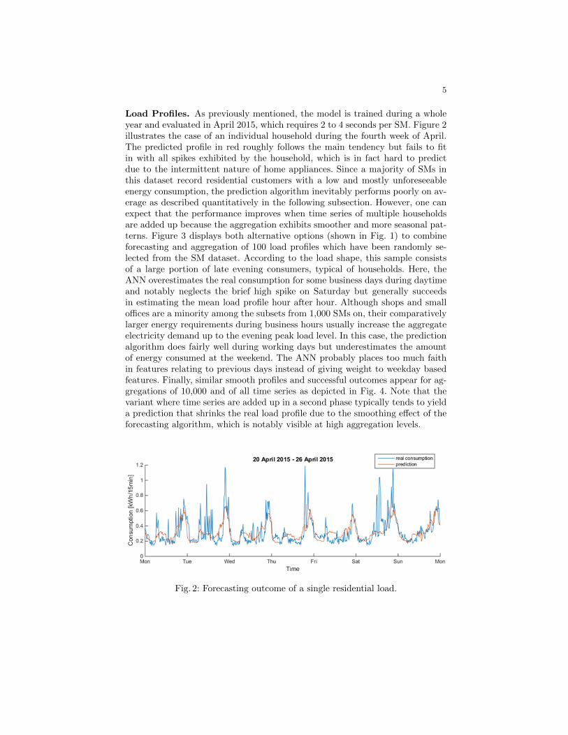
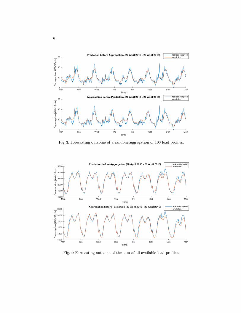
Spatial Aggregation. Besides training a model on single time series, differentaggregation sizes are investigated, i.e. the aggregation of 10, 100, 1,000, 10,000and all load profiles. Two options can be implemented which are presented inFig. 1 with an example of 10 SMs:

(a) The forecast is carried out for each single profile before building groups of10 randomly chosen predicted time series and adding them up,

(b) Original time series are first added up according to the previous group forma-tion and the forecasting algorithm is only applied to aggregate load profiles.

(a) (b)

Fig. 1: Two versions to perform prediction with an aggregation of 10 load profiles.

5

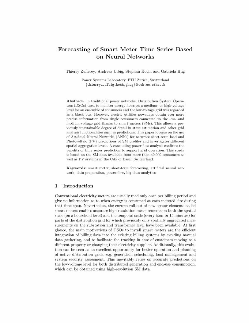
Load Profiles. As previously mentioned, the model is trained during a wholeyear and evaluated in April 2015, which requires 2 to 4 seconds per SM. Figure 2illustrates the case of an individual household during the fourth week of April.The predicted profile in red roughly follows the main tendency but fails to fitin with all spikes exhibited by the household, which is in fact hard to predictdue to the intermittent nature of home appliances. Since a majority of SMs inthis dataset record residential customers with a low and mostly unforeseeableenergy consumption, the prediction algorithm inevitably performs poorly on av-erage as described quantitatively in the following subsection. However, one canexpect that the performance improves when time series of multiple householdsare added up because the aggregation exhibits smoother and more seasonal pat-terns. Figure 3 displays both alternative options (shown in Fig. 1) to combineforecasting and aggregation of 100 load profiles which have been randomly se-lected from the SM dataset. According to the load shape, this sample consistsof a large portion of late evening consumers, typical of households. Here, theANN overestimates the real consumption for some business days during daytimeand notably neglects the brief high spike on Saturday but generally succeedsin estimating the mean load profile hour after hour. Although shops and smalloffices are a minority among the subsets from 1,000 SMs on, their comparativelylarger energy requirements during business hours usually increase the aggregateelectricity demand up to the evening peak load level. In this case, the predictionalgorithm does fairly well during working days but underestimates the amountof energy consumed at the weekend. The ANN probably places too much faithin features relating to previous days instead of giving weight to weekday basedfeatures. Finally, similar smooth profiles and successful outcomes appear for ag-gregations of 10,000 and of all time series as depicted in Fig. 4. Note that thevariant where time series are added up in a second phase typically tends to yielda prediction that shrinks the real load profile due to the smoothing effect of theforecasting algorithm, which is notably visible at high aggregation levels.

Fig. 2: Forecasting outcome of a single residential load.

6

Fig. 3: Forecasting outcome of a random aggregation of 100 load profiles.

Fig. 4: Forecasting outcome of the sum of all available load profiles.

7

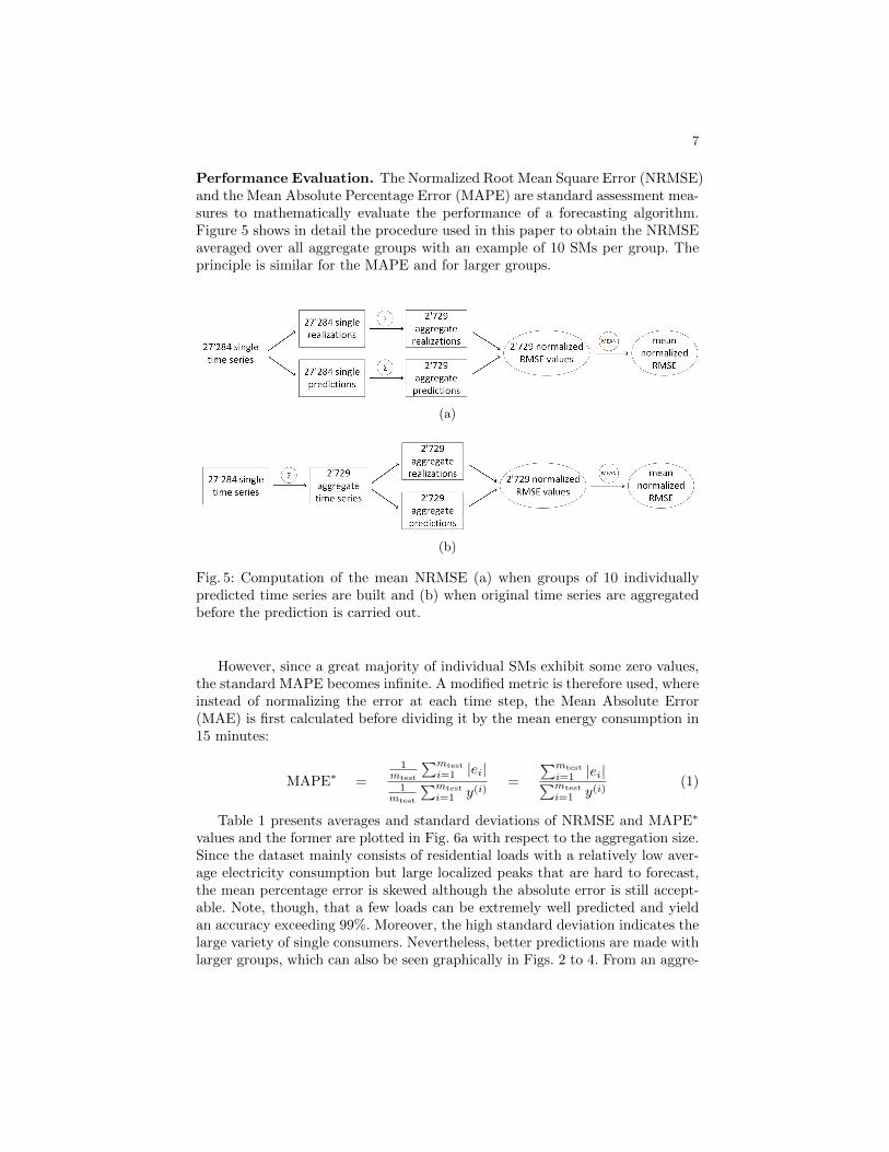
Performance Evaluation. The Normalized Root Mean Square Error (NRMSE)and the Mean Absolute Percentage Error (MAPE) are standard assessment mea-sures to mathematically evaluate the performance of a forecasting algorithm.Figure 5 shows in detail the procedure used in this paper to obtain the NRMSEaveraged over all aggregate groups with an example of 10 SMs per group. Theprinciple is similar for the MAPE and for larger groups.

(a)

(b)

Fig. 5: Computation of the mean NRMSE (a) when groups of 10 individuallypredicted time series are built and (b) when original time series are aggregatedbefore the prediction is carried out.

However, since a great majority of individual SMs exhibit some zero values,the standard MAPE becomes infinite. A modified metric is therefore used, whereinstead of normalizing the error at each time step, the Mean Absolute Error(MAE) is first calculated before dividing it by the mean energy consumption in15 minutes:

MAPE∗ =1

mtest

∑mtest

i=1 |ei|1

mtest

∑mtest

i=1 y(i)=

∑mtest

i=1 |ei|∑mtest

i=1 y(i)(1)

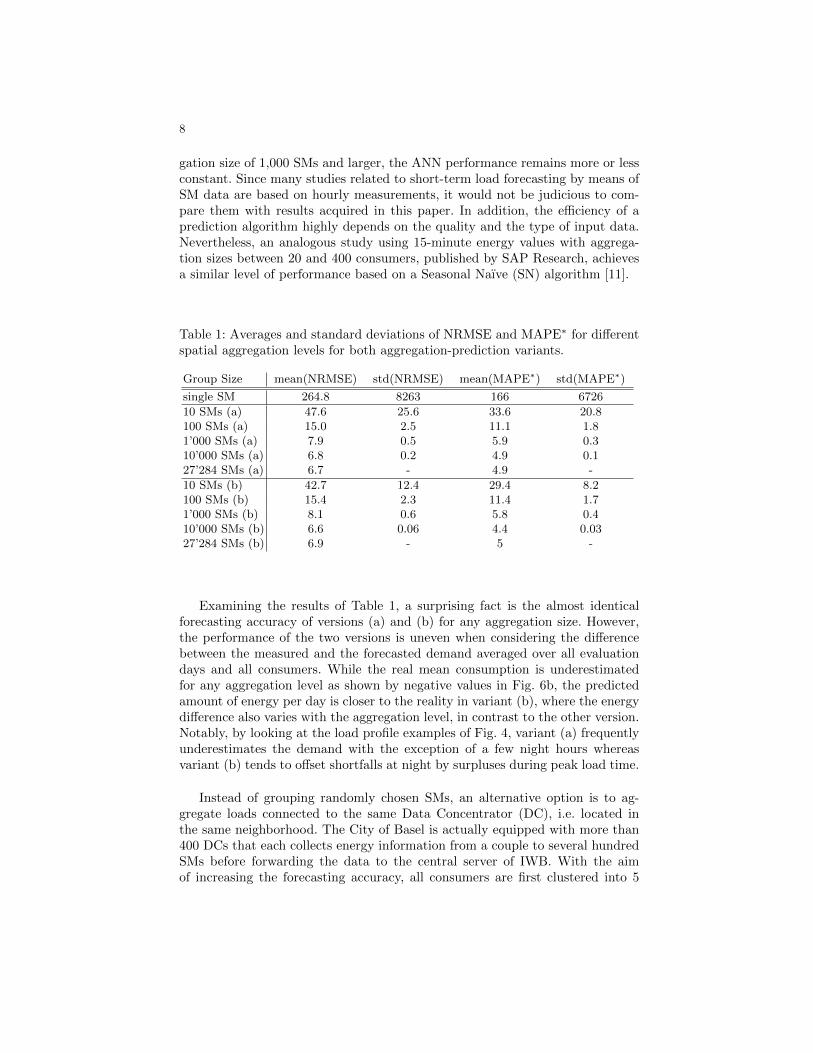
Table 1 presents averages and standard deviations of NRMSE and MAPE∗

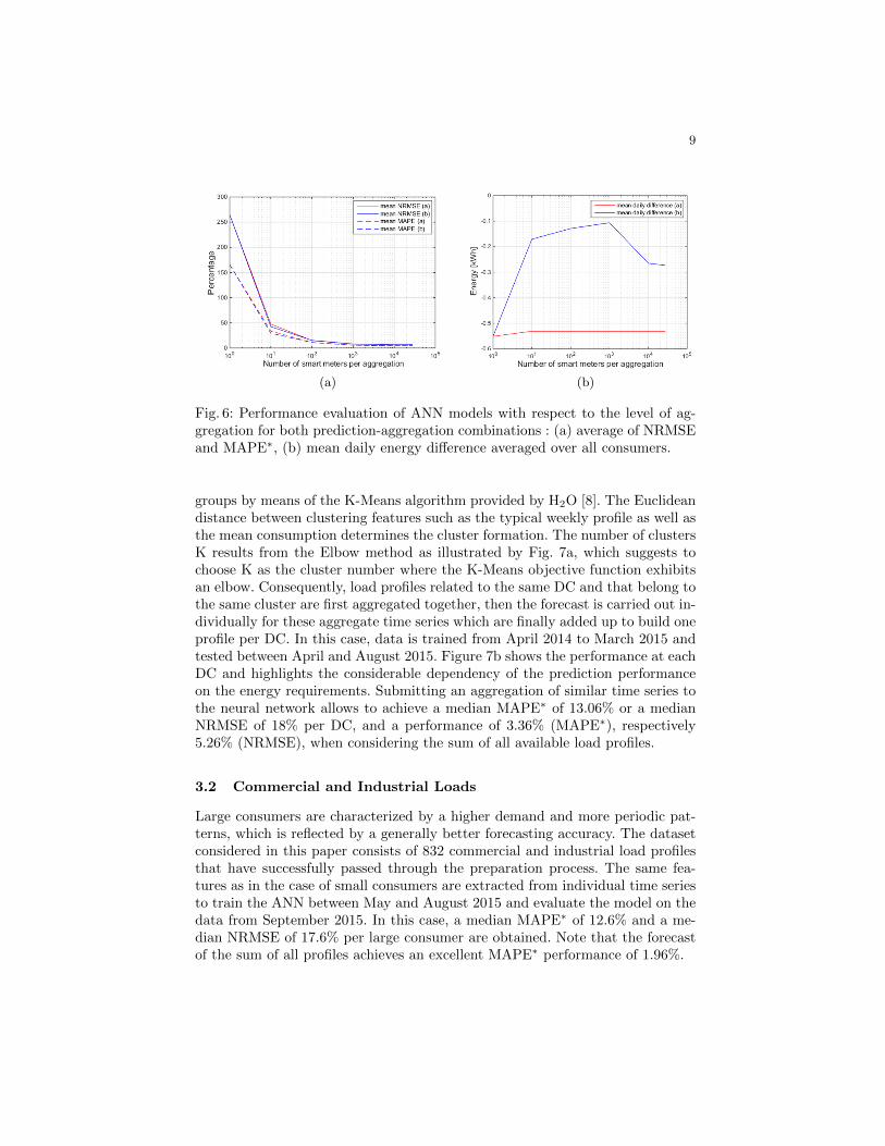
values and the former are plotted in Fig. 6a with respect to the aggregation size.Since the dataset mainly consists of residential loads with a relatively low aver-age electricity consumption but large localized peaks that are hard to forecast,the mean percentage error is skewed although the absolute error is still accept-able. Note, though, that a few loads can be extremely well predicted and yieldan accuracy exceeding 99%. Moreover, the high standard deviation indicates thelarge variety of single consumers. Nevertheless, better predictions are made withlarger groups, which can also be seen graphically in Figs. 2 to 4. From an aggre-

8

gation size of 1,000 SMs and larger, the ANN performance remains more or lessconstant. Since many studies related to short-term load forecasting by means ofSM data are based on hourly measurements, it would not be judicious to com-pare them with results acquired in this paper. In addition, the efficiency of aprediction algorithm highly depends on the quality and the type of input data.Nevertheless, an analogous study using 15-minute energy values with aggrega-tion sizes between 20 and 400 consumers, published by SAP Research, achievesa similar level of performance based on a Seasonal Naıve (SN) algorithm [11].

Table 1: Averages and standard deviations of NRMSE and MAPE∗ for differentspatial aggregation levels for both aggregation-prediction variants.

Group Size mean(NRMSE) std(NRMSE) mean(MAPE∗) std(MAPE∗)

single SM 264.8 8263 166 6726

10 SMs (a) 47.6 25.6 33.6 20.8100 SMs (a) 15.0 2.5 11.1 1.81’000 SMs (a) 7.9 0.5 5.9 0.310’000 SMs (a) 6.8 0.2 4.9 0.127’284 SMs (a) 6.7 - 4.9 -

10 SMs (b) 42.7 12.4 29.4 8.2100 SMs (b) 15.4 2.3 11.4 1.71’000 SMs (b) 8.1 0.6 5.8 0.410’000 SMs (b) 6.6 0.06 4.4 0.0327’284 SMs (b) 6.9 - 5 -

Examining the results of Table 1, a surprising fact is the almost identicalforecasting accuracy of versions (a) and (b) for any aggregation size. However,the performance of the two versions is uneven when considering the differencebetween the measured and the forecasted demand averaged over all evaluationdays and all consumers. While the real mean consumption is underestimatedfor any aggregation level as shown by negative values in Fig. 6b, the predictedamount of energy per day is closer to the reality in variant (b), where the energydifference also varies with the aggregation level, in contrast to the other version.Notably, by looking at the load profile examples of Fig. 4, variant (a) frequentlyunderestimates the demand with the exception of a few night hours whereasvariant (b) tends to offset shortfalls at night by surpluses during peak load time.

Instead of grouping randomly chosen SMs, an alternative option is to ag-gregate loads connected to the same Data Concentrator (DC), i.e. located inthe same neighborhood. The City of Basel is actually equipped with more than400 DCs that each collects energy information from a couple to several hundredSMs before forwarding the data to the central server of IWB. With the aimof increasing the forecasting accuracy, all consumers are first clustered into 5

9

(a) (b)

Fig. 6: Performance evaluation of ANN models with respect to the level of ag-gregation for both prediction-aggregation combinations : (a) average of NRMSEand MAPE∗, (b) mean daily energy difference averaged over all consumers.

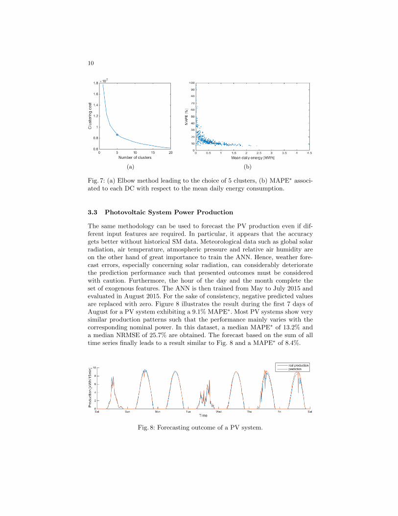
groups by means of the K-Means algorithm provided by H2O [8]. The Euclideandistance between clustering features such as the typical weekly profile as well asthe mean consumption determines the cluster formation. The number of clustersK results from the Elbow method as illustrated by Fig. 7a, which suggests tochoose K as the cluster number where the K-Means objective function exhibitsan elbow. Consequently, load profiles related to the same DC and that belong tothe same cluster are first aggregated together, then the forecast is carried out in-dividually for these aggregate time series which are finally added up to build oneprofile per DC. In this case, data is trained from April 2014 to March 2015 andtested between April and August 2015. Figure 7b shows the performance at eachDC and highlights the considerable dependency of the prediction performanceon the energy requirements. Submitting an aggregation of similar time series tothe neural network allows to achieve a median MAPE∗ of 13.06% or a medianNRMSE of 18% per DC, and a performance of 3.36% (MAPE∗), respectively5.26% (NRMSE), when considering the sum of all available load profiles.

3.2 Commercial and Industrial Loads

Large consumers are characterized by a higher demand and more periodic pat-terns, which is reflected by a generally better forecasting accuracy. The datasetconsidered in this paper consists of 832 commercial and industrial load profilesthat have successfully passed through the preparation process. The same fea-tures as in the case of small consumers are extracted from individual time seriesto train the ANN between May and August 2015 and evaluate the model on thedata from September 2015. In this case, a median MAPE∗ of 12.6% and a me-dian NRMSE of 17.6% per large consumer are obtained. Note that the forecastof the sum of all profiles achieves an excellent MAPE∗ performance of 1.96%.

10

(a) (b)

Fig. 7: (a) Elbow method leading to the choice of 5 clusters, (b) MAPE∗ associ-ated to each DC with respect to the mean daily energy consumption.

3.3 Photovoltaic System Power Production

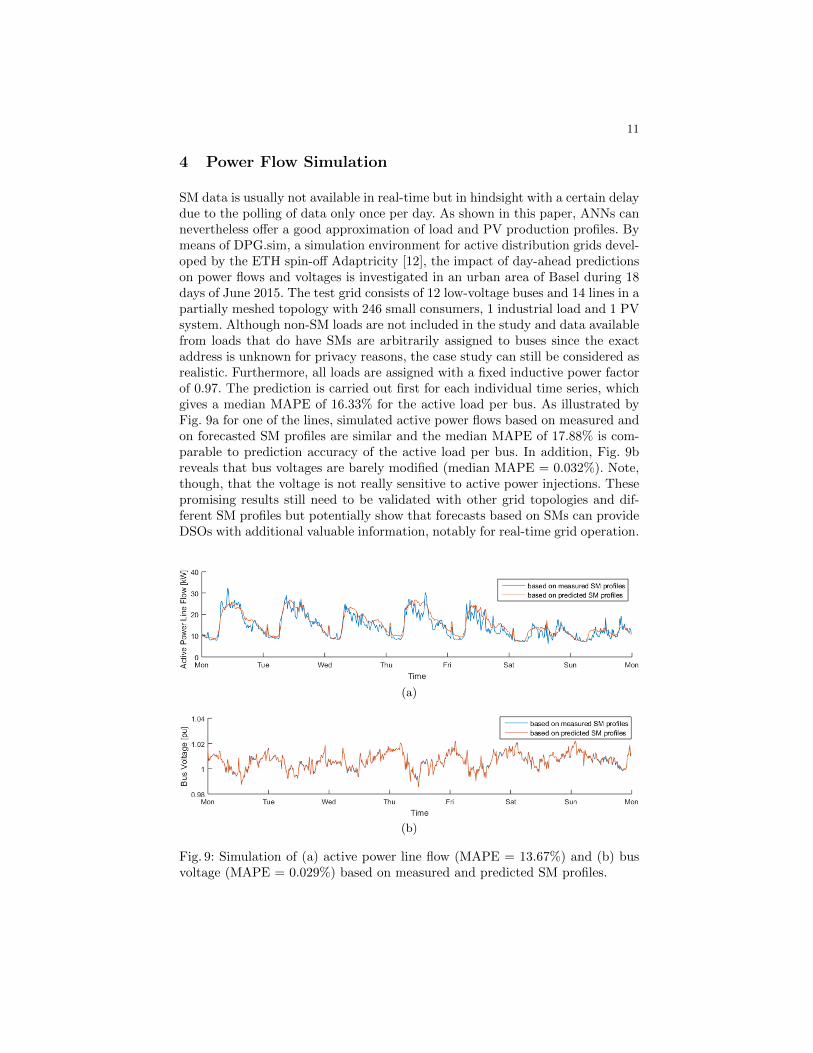
The same methodology can be used to forecast the PV production even if dif-ferent input features are required. In particular, it appears that the accuracygets better without historical SM data. Meteorological data such as global solarradiation, air temperature, atmospheric pressure and relative air humidity areon the other hand of great importance to train the ANN. Hence, weather fore-cast errors, especially concerning solar radiation, can considerably deterioratethe prediction performance such that presented outcomes must be consideredwith caution. Furthermore, the hour of the day and the month complete theset of exogenous features. The ANN is then trained from May to July 2015 andevaluated in August 2015. For the sake of consistency, negative predicted valuesare replaced with zero. Figure 8 illustrates the result during the first 7 days ofAugust for a PV system exhibiting a 9.1% MAPE∗. Most PV systems show verysimilar production patterns such that the performance mainly varies with thecorresponding nominal power. In this dataset, a median MAPE∗ of 13.2% anda median NRMSE of 25.7% are obtained. The forecast based on the sum of alltime series finally leads to a result similar to Fig. 8 and a MAPE∗ of 8.4%.

Fig. 8: Forecasting outcome of a PV system.

11

4 Power Flow Simulation

SM data is usually not available in real-time but in hindsight with a certain delaydue to the polling of data only once per day. As shown in this paper, ANNs cannevertheless offer a good approximation of load and PV production profiles. Bymeans of DPG.sim, a simulation environment for active distribution grids devel-oped by the ETH spin-off Adaptricity [12], the impact of day-ahead predictionson power flows and voltages is investigated in an urban area of Basel during 18days of June 2015. The test grid consists of 12 low-voltage buses and 14 lines in apartially meshed topology with 246 small consumers, 1 industrial load and 1 PVsystem. Although non-SM loads are not included in the study and data availablefrom loads that do have SMs are arbitrarily assigned to buses since the exactaddress is unknown for privacy reasons, the case study can still be considered asrealistic. Furthermore, all loads are assigned with a fixed inductive power factorof 0.97. The prediction is carried out first for each individual time series, whichgives a median MAPE of 16.33% for the active load per bus. As illustrated byFig. 9a for one of the lines, simulated active power flows based on measured andon forecasted SM profiles are similar and the median MAPE of 17.88% is com-parable to prediction accuracy of the active load per bus. In addition, Fig. 9breveals that bus voltages are barely modified (median MAPE = 0.032%). Note,though, that the voltage is not really sensitive to active power injections. Thesepromising results still need to be validated with other grid topologies and dif-ferent SM profiles but potentially show that forecasts based on SMs can provideDSOs with additional valuable information, notably for real-time grid operation.

(a)

(b)

Fig. 9: Simulation of (a) active power line flow (MAPE = 13.67%) and (b) busvoltage (MAPE = 0.029%) based on measured and predicted SM profiles.

12

5 Conclusion

Based on a large database, this paper proposes an exhaustive approach for fore-casting various types of SM profiles, from an appropriate data preparation tothe use of predicted time series in a power flow study. While an individualhousehold is difficult to forecast, a considerably improved accuracy is achievedfor commercial and industrial loads, PV systems and aggregate load profiles.Furthermore, training an ANN on spatially aggregated time series instead ofadding up individual predicted profiles allows to reduce the computational costwithout decreasing the forecasting accuracy. An even better efficiency can stillbe obtained by aggregating profiles of similar shapes. It would be neverthelessworthwhile to consider longer training and validation periods and investigateother prediction algorithms on this type of data, e.g. Support Vector Machine(SVM) or more sophisticated ANNs like Recurrent Neural Network (RNN) andLong Short-Term Memory (LSTM). In addition, the impact of weather forecasterrors should be closely assessed. Eventually, based on satisfactory SM predic-tions, DSOs would be able to gain insight into the state of their low-voltage gridin real-time even though real-time measurements are not directly available.

Acknowledgements. This study is part of the project “Optimized DistributionGrid Operation by Utilization of SmartMetering Data” funded by the SwissFederal Office of Energy and carried out at the ETH Zurich in collaborationwith the ETH spin-off company Adaptricity [12] and the public utility of theCity of Basel “Industrielle Werke Basel” (IWB).

References

1. Industrielle Werke Basel, http://www.iwb.ch/2. MeteoSwiss, http://www.meteoswiss.admin.ch3. Troyanskaya, O., Cantor, M., Sherlock, G., Brown, P., Hastie, T., Tibshirani, R.,

Botstein, D., Altman, R.B.: Missing value estimation methods for DNA microar-rays. In: Bioinformatics 17(6), pp. 520–525. Oxford Univ Press (2001)

4. Alcal-Fdez, J., Snchez, L. , Garca, S., Del Jesus, M., Ventura, S., Garrell, J., Otero,J., Romero, C., Bacardit, J., Rivas, V., Fernndez, J., Herrera, F.: Knowledge Ex-traction based on Evolutionary Learning, http://sci2s.ugr.es/keel/algorithms.php

5. Apache Spark, https://spark.apache.org6. Koponen, P., Mutanen, A., Niska, H.: Assessment of Some Methods for Short-Term

Load Forecasting. In: IEEE PES ISGT Europe (2014)7. He, W.: Deep neural network based load forecast. In: Computer Modelling & New

Technologies 2014 18(3), pp. 258–2628. OxData H2O, http://www.h2o.ai9. Valtonen, P., Honkapuro, S., Partanen, J.: Improving Short-Term Load Forecast

Accuracy by Utilizing Smart Metering. In: CIRED Workshop, Lyon, France (2010)10. Busseti, E., Osband, I., Wong, S.: Deep Learning for Time Series Modeling. In: CS

229 Final Project Report. Stanford University (2012)11. Ilic, D., Karnouskos, S., Da Silva, P. G.: Improving Load Forecast in Prosumer

Clusters by Varying Energy Storage Size. In: IEEE Grenoble PowerTech (2013)12. Adaptricity AG, https://www.adaptricity.com