Forecasting Market Prices in a Supply Chain Game

Christopher Kiekintveld a, Jason Miller b, Patrick R. Jordan a,Lee F. Callender a, and Michael P. Wellman a

aUniversity of MichiganComputer Science and Engineering

Ann Arbor, MI 48109-2121 USAbStanford University

Department of Mathematics, building 380Stanford, CA 94305 USA

Abstract

Predicting the uncertain and dynamic future of market conditions on the supply chain, asreflected in prices, is an essential component of effective operational decision making. Wepresent and evaluate methods used by our agent, Deep Maize, to forecast market prices inthe Trading Agent Competition Supply Chain Management game (TAC/SCM). We employa variety of machine learning and representational techniques to exploit as many typesof information as possible, integrating well-known methods in novel ways. We evaluatethese techniques through controlled experiments as well as performance in both the mainTAC/SCM tournament and supplementary Prediction Challenge. Our prediction methodsdemonstrate strong performance in controlled experiments and achieved the best overallscore in the Prediction Challenge.

? This is a revised and substantially extended version of a paper presented at the SixthInternational Joint Conference on Autonomous Agents and Multiagent Systems [23].

Email addresses: ckiekint@umich.edu (Christopher Kiekintveld),jmiller@math.stanford.edu (Jason Miller), prjordan@umich.edu (PatrickR. Jordan), asleep@umich.edu (Lee F. Callender), wellman@umich.edu(Michael P. Wellman).

URLs: http://teamcore.usc.edu/kiekintveld (Christopher Kiekintveld),http://www.eecs.umich.edu/˜prjordan (Patrick R. Jordan),http://ai.eecs.umich.edu/people/wellman (Michael P. Wellman).

Preprint submitted to Elsevier 3 November 2008

1 Introduction

The quality of economic decisions made now depend on market conditions thatwill prevail in the future. This is particularly true of supply chain environments,which evolve dynamically based on complex interactions among multiple play-ers across several tiers. We present and evaluate methods of forecasting marketconditions developed to predict prices in the Trading Agent Competition SupplyChain Management game (TAC/SCM). In TAC/SCM, automated trading agentscompete to maximize their profits in a simulated supply-chain environment. Theyface many challenges, including strategic interactions and uncertainty about marketconditions. Though complex, this domain offers a relatively controlled environmentamenable to extensive experimentation. TAC also attracts a diverse pool of partici-pants, which facilitates benchmarking and evaluation. This is particularly importantfor prediction tasks, where the quality of predictions depends in part on the actionsof opponents. Research competitions such as TAC offer the opportunity to test pre-dictions in environments where the opposing agents are designed and selected byothers, mitigating an important source of potential bias relative to using opponentsof one’s own design [37].

Our agent for the SCM game, Deep Maize, relies on price predictions in boththe upstream and downstream markets to make purchasing, production, and salesdecisions. Figure 1 shows an overview of the daily decision process. Predictionsabout market conditions feed into an approximate optimization procedure that usesvalues to decompose the decision problem. The architecture is described in detailelsewhere [22]. Since our predictions are integrated into a task-situated agent, wecan evaluate the benefits of improved predictions on overall performance in addi-tion to prediction error metrics.

We apply machine learning to forecast prices in two different markets with distinctnegotiation mechanisms and information-revelation rules. Like many real markets,the available information on market conditions comes from a variety of hetero-geneous sources. Integrating different learning techniques and representations toexploit all of the available information is a central theme of our approach. We findthat representing the current market conditions well is particularly important foreffective learning.

We begin with a discussion of related work and an overview of the TAC/SCMgame, highlighting the benefits and drawbacks of the different forms of informa-tion available for making predictions. The first set of methods we describe are usedfor predicting prices in the downstream consumer market. Central to all of thesemethods is a nearest-neighbors learning algorithm that uses historical game datato induce the relationship between market indicators and prices. We test variationsthat employ two different representations for price distributions: an absolute rep-resentation, and a relative representation that exploits local price stability. Finally,

2

State State Estimation

Long-termProduction Schedule

Supply Supply MarketMarket

PredictionPrediction

CustomerCustomerMarket Market

PredictionPrediction

Market Predictions

ComponentValues

PCValues

CustomerSales

SupplyPurchasing

FactorySchedule

High-levelDecisions

Low-levelDecisions

Fig. 1. Overview of Deep Maize’s decision process on each TAC/SCM day.

we develop an online learning method that procedure that combines and shifts pre-dictions using additional observations within a game instance. Our evaluation ofthese methods includes both prediction error and supply-chain performance. Weshow substantial improvements over a baseline predictor, with online adaptationexhibiting especially strong performance improvements.

We proceed to discuss methods for making predictions in the market for compo-nent supplies. There are two elements to our approach in this market. The first is alinear interpolation model that uses recent observations to make relatively accuratepredictions about the current spot market. The second is a learning model that re-gresses prices against market indicators. This learning model can be used to makeabsolute price predictions, or to predict residuals for the linear interpolation model.We show that combining the linear interpolation model for current market priceswith residual predictions improves overall performance, particularly for long-termpredictions.

We close with discussion of the performance of both prediction algorithms basedon the results of TAC/SCM tournaments and the inaugural TAC/SCM PredictionChallenge. Deep Maize has been a perennial finalist in the primary competition,and placed first in the Prediction Challenge. Our forecasting methods demonstratestrong performance on prediction error measures and contribute to strong overallperformance in the context of decision making.

3

2 Related Work

Forecasting is studied across many disciplines, and many approaches have beendeveloped for making predictions based on historical data. We do not attempt tosurvey all of the various methods here, but refer the reader to one of many introduc-tory texts that describe exponential smoothing, GARCH, ARIMA, spectral analy-sis, neural networks, Kalman filters, and other popular methods [5,8,15]. Pindyckand Rubinfeld [33] is a good introduction to many forecasting methods used in thecontext of economic predictions and modeling. The proliferation of techniques isin part an indication that the best method for any particular problem may dependon many factors, including the type and quantity of information available and theproperties of the domain.

Many applications focus on comparing methods to identify the most effective ap-proach for a particular problem (for example, see the application of forecasting toretail sales by Alon et al. or the application to predict electricity prices by Nogaleset al. [26]). Our approach for price prediction focuses on combining predictionsmade using difference sources of information and methods. Various methods havebeen developed for combining predictions, often motivated by the problem of com-bining the opinions of experts [1,10]. Recently, predictions markets have become apopular method for aggregating information [14]. Our approach shares some fea-tures with these markets, including the use of logarithmic scoring rules to evaluatethe quality of predictions.

Price forecasting is a very important element of decision making in a wide varietyof market settings, including financial markets [18] and energy markets [26]. Therise of internet auctions has led to an increasing interest in computational methodsfor price forecasting in auction environments (e.g., [13]). Brooks et al. [6] discussesmany issues related to learning price models in the context of online markets. Priceprediction methods have also been used as the basis for successful bidding strate-gies in many specific types of auctions, including simultaneous ascending auctions[27]. It is not surprising then that price prediction has played an important role in thedesign of agents for the Trading Agent Competition since its inception. For the TACTravel game [37], a crucial factor in agent performance was the ability to predict theclosing price of auctions for hotel rooms. Participants explored many approachesfor making these predictions, spanning statistical analysis, machine learning, andeconomic modeling [9,36,38]. Post-tournament analysis revealed that the commonthread among the most effective methods was not the particular technique applied,but rather the information taken into account by the predictor [38]; specifically, thebest predictors accounted for the initial auction prices.

Most agents for the TAC/SCM game also employ some form of price prediction,but vary significantly both in what quantities are predicted and the methods usedfor making predictions. Many agents only estimate prices for the current simulation

4

day, and do not attempt to forecast changes in prices over time [2,3,7,16]. One ofthe most successful agents in the tournament, TacTex, has applied a variety of so-phisticated approaches for price prediction. The specific methods have evolved insuccessive tournaments, but generally rely on a combination of statistical machinelearning applied to historical data and online adaptation [29–32]. The most recentversion of TacTex specifically uses machine learning to predict both current and fu-ture prices. The MinneTAC team has also devoted significant effort to developingprediction methods for the TAC/SCM domain [20,21]. Their approach is somewhatunique in that it focus on predicting changes in the economic regimes, which re-flect over-supply, under-supply, or other characteristic market conditions. Our useof market state is similar in spirit to the idea of an economic regime, but we donot distinguish among a discrete set of possible regimes. The first version of DeepMaize used an analytic solution based on competitive equilibrium to predict marketprices [25]. This approach became infeasible when the game rules were modifieddue to the greater complexity of the supplier pricing model. Another unique ap-proach was used by RedAgent, the winner of the first TAC/SCM competition [19].This agent used an internal market to coordinate decisions and make predictions;to our knowledge no current agents use this approach.

3 The TAC Supply-Chain Game

Agent 1

Agent 2

Agent 4

Agent 3

Agent 5

Agent 6

Pintel

IMD

Basus

Macrostar

Mec

Queenmax

Watergate

Mintor

supplieroffer

componentRFQ

offeracceptance

Customerbid

PC RFQ

CP

UM

oth

erboar

dM

emory

Har

d D

isk

Fig. 2. TAC/SCM supply chain configuration.

5

Agents in TAC/SCM play the role of personal computer (PC) manufacturers [11,12]. 1

The six automated agents compete to maximize their profits on a simulated supplychain, shown in Figure 2. Agents assemble 16 different types of PCs for sale, de-fined by compatible combinations of CPU, motherboard, hard disk, and memorycomponents. Each day agents negotiate with suppliers to purchase components,negotiate with customers to sell finished products, and create manufacturing andshipping schedules for the next day. Each agent has an identical factory with lim-ited capacity for production. Each game has 220 simulated days, each of whichtakes 15 seconds of real time.

3.1 The Personal Computer Market

The 16 PC types are separated into three market segments representing high-, mid-,and low-grade PCs. The average demand level for each segment varies separatelyaccording to a random walk with a stochastic trend. Each day, the customer demandprocess generates a set of RFQs (request-for-quotes) representing the aggregatedemand. Each customer request is valid for a single day and specifies a PC type,due date, reserve price, and penalty for late delivery. The negotiations for theserequests use a simultaneous sealed-bid auction mechanism. Agents submit priceoffers for a subset of the RFQs. The lowest bidder for each request is awarded theorder, and must deliver the product by the due date or pay the penalty specified inthe contract. Due to the configuration of the market, there are strong interactionsamong auctions both within and across days.

3.2 The Component Market

To procure components to build PCs, agents must negotiate with eight supplierswhose behavior is defined in the game specification. Each supplier sells two dis-tinct grades of a single component type. CPU components have a unique supplier,whereas all other types are provided by two suppliers. Suppliers have a limiteddaily production capacity for each component they sell. These capacities vary ac-cording to a mean-reverting random walk, and are not directly observable by themanufacturers.

Manufacturers negotiate with suppliers via an RFQ mechanism. Each day, a manu-facturer may send up to five RFQs per component to each supplier specifying type,due date, quantity, and reserve price. Any future day may be specified as the duedate. The suppliers respond the following day with offers specifying a proposed

1 We present an overview of the game rules here. The full rule specifications for eachcompetition, tournament results, and general TAC information are available at http://www.sics.se/tac.

6

quantity, price, and delivery date. 2 Suppliers may opt to accept a subset of theoffers by responding with orders. Suppliers determine offer prices based on theratio of their committed and available production capacity. This pricing functionaccounts for inventory, previous commitments, future capacity, and the demandrepresented in the current set of customer RFQs. In general, component prices riseas demand rises and suppliers become more constrained. In some cases, the sup-plier may be capacity constrained and unable to offer components at any price.Prices depend on both the requested due date and the day the request is made. Pricepredictions must be made for this entire space of possibilities to support importantdecisions about the optimal time to make component purchases.

3.3 Observable Market Data

Agents may utilize several complementary forms of evidence to make predictionsabout market prices. Each provides unique insights into current activity and howthe market may evolve. The first category of evidence comprises observations ofthe markets during a game instance. This information is the most timely and spe-cific to the current situation, but is of relatively low fidelity. More detailed obser-vations of market activity are available in game logs after each game instance hascompleted. 3 Logs from previous rounds are publicly available, and additional datamay be generated in private simulations.

During a game, agents receive daily observations from participating in the PCand component markets. In the PC market, agents observe the set of requests andwhether or not each bid resulted in an order. They also receive a daily report foreach PC type listing the maximum and minimum selling price from the previousday. The details of individual market transactions and opponents’ bids are not re-vealed. In the component market, agents receive price quotes for each request theysend, some of which may be price probes. Neither the supplier’s state (inventory,capacity, and commitments) nor other agents’ requests are revealed. Every 20 sim-ulation days, manufacturers receive a report containing aggregate market data forthe preceding 20-day period. This data includes the mean selling price and quantitysold for each PC type, and the mean selling price, quantity ordered, and quantityshipped for component type. The report also includes the mean production capac-ity for each supply line. The importance of this evidence is that it is specific to thecurrent market conditions and current set of manufacturing agents. However, theseobservations say relatively little about how market conditions are likely to evolve,especially if similar conditions have not been observed earlier in the game.

2 Suppliers may offer either a partial quantity or a later delivery if they are unable to meetthe initial request due to capacity constraints.3 A rule change in 2007 explicitly disallows agents from collecting and utilizing these logsduring a tournament round, but logs from previous rounds or simulations may still be used.

7

Table 1Four categories of predictions made in the Prediction Challenge.

Prediction Description

Current PC prices Lowest price offered by manufacturers for each current RFQ

Future PC prices Median lowest price offered for each PC type in 20 days

Current component prices Offer price for each component RFQ sent on current day

Future component prices Offer price for each component RFQ sent in 20 days

The historical logs reveal the entire transaction history in each market (includingall bids, offers, and orders), as well as supplier capacities and other state attributeshidden during a game instance. This precise information is potentially very usefulfor predicting the evolution of market prices over time. However, conditions in thecurrent game are unlikely to be identical to conditions in historical games. A partic-ularly difficult issue is that the pool of competing agents is constantly changing asteams update their agents, so historical data may not be representative of the currentstrategic environment. Selecting relevant historical data is an important challenge.

3.4 The Prediction Challenge

The 2007 TAC event introduced two challenge competitions to complement theoriginal TAC/SCM scenario. In the TAC/SCM Prediction Challenge [28], agentscompete to make the most accurate price predictions in four categories: short- andlong-term, for both component and PC markets (see Table 1). The challenge iso-lates the prediction component of the game by having participants make predictionson behalf of the same designated agent, PAgent. Simulations including a PAgentare run before the challenge to generate log files. During the challenge, the log filesare used to simulate the experience of playing the game for the predictors by pro-viding the exact sequence of messages observed by PAgent during the game. Thepredictions made based on this information by competitors in the Challenge do notaffect the behavior of the PAgent. This simulation framework allows all predictorsto make an identical set of predictions, and also allows predictions to be made manytimes for the same set of game instances. The predictions are scored against actualprices using the root mean squared (RMS) error, normalizing by component andPC base prices.

Each round of the challenge used three sets of 16 game instances, with differentagents competing with PAgent on the supply chain. The agents comprising thecompetitive environment were selected from those in the public agent repository. 4

4 The TAC agent repository http://www.sics.se/tac/showagents.php storesbinary implementations of many agents from past TAC tournaments, released by their de-velopers.

8

Since tests can be run independently and repeated, the software framework for theChallenge also provides a useful toolkit for conducting one’s own prediction tests.We took advantage of this in developing and testing new prediction methods for thecomponent market in preparation for the 2007 TAC/SCM tournament and Predic-tion Challenge.

4 Methods for PC Market Predictions

Each day, Deep Maize estimates the underlying demand state in the customer mar-ket and creates predictions of the price curves it faces. 5 For the current simulationday, the set of requests is known. Estimating the price curve in this case is equiv-alent to estimating the probability that a given bid on an RFQ will result in anorder, denoted Pr(win|bid). To predict the price curve for future simulation days,it is also necessary to predict the set of request that will be generated. We combinepredictions about the set of requests and the distribution of selling prices for eachrequest (i.e., Pr(win|bid)) to estimate the effective demand curve for each futureday. The effective demand curve represents the expected marginal selling prices foreach additional PC sold. The agent uses these forecast demand curves to make cus-tomer bidding decisions and create a projected manufacturing schedule. We beginby discussion of our methods for estimating a key element of the game state, andproceed with a discussion of our methods for predicting customer market prices.

4.1 Customer Demand Projection

The customer demand processes that determine the number of RFQs to generateexert a great influence on market prices in the SCM game. There are three stochasticdemand processes, corresponding to the respective market segments. Each processis captured by two state variables: a mean Q and trend τ . The number of RFQsgenerated in each market segment on day d is determined by a draw from a Poissondistribution with mean Q. The initial demand levels for each segment are drawnuniformly from known intervals. The mean demand evolves according to the dailyupdate rule

Qd+1 = min(Qmax,max(Qmin, τdQd)). (1)

Both the minimum and maximum values of Q are given for each market segmentin the specification. The trend τ is initially neutral, τ0 = 1, and is updated by the

5 The methods described in this section were developed for the 2005 TAC/SCM tourna-ment, and used with minor updates and new data sets in the 2006 competition. The versionused in the 2007 tournament and Prediction Challenge were identical to the 2006 version(including the data sets).

9

stochastic perturbation ε ∼ U [−0.01, 0.01]:

τd+1 = max(0.95,min(1/0.95, τd + ε)). (2)

When the demand Q reaches a maximum or minimum value, the trend resets to theneutral level.

Qd

τd

Qd+1

#Q

τd+1

Fig. 3. Bayesian network model of demand evolution.

The stateQ and τ are hidden from the manufacturers, but can be estimated based onthe observed demand. We estimate the underlying demand process using a Bayesianmodel, illustrated in Figure 3. 6 Note that the updated demand,Qd+1, is a determin-istic function of Qd and τd, as specified in Eq. (1). This deterministic relationshipsimplifies the update of our beliefs about the demand state given a new observa-tion. Let Pr(Qd, τd) denote the probability distribution over demand states givenour observations through day d. We can incorporate a new observation Qd+1 asfollows:

Pr(Qd, τd|Qd+1) ∝ Pr(Qd+1|Qd, τd) Pr(Qd, τd). (3)

Eq. (3) exploits the fact that the observation at d+1 is conditionally independent ofprior observations given the demand state (Qd, τd). We can elaborate the first termof the RHS using the demand update (1):

Pr(Qd+1|Qd, τd) = Poisson(min(Qmax,max(Qmin, τdQd))).

After calculating the RHS of Eq. (3) for all possible demand states, we normalizeto recover the updated probability distribution. We can then project forward ourbeliefs over (Qd, τd) using the demand and trend update equations (1) and (2), toobtain a probability distribution over (Qd+1, τd+1).

A sequence of updates by Eq. (3) represents an exact posterior distribution overdemand state given a series of observations. To maintain a finite encoding of thisjoint distribution, we consider only integer values for demand and divide the trend

6 We have released source code for this estimation method. It is available in the TAC agentrepository.

10

range into T discrete values, evenly spaced (Deep Maize uses T = 9 for tourna-ment play). Given a distribution over demand states, we can project this distributionforward to estimate future demand.

4.2 Learning Prices from Historical Data

We use a k-nearest neighbors (kNN) algorithm to induce the relationship betweenindicators of market conditions (features) and likely distributions of current andfuture prices. The idea is simple: given a set of games, find situations that mostclosely resemble the current situation and predict based on the observed outcomes.When prices are not changing much from day to day, learning prices from historicaldata has little additional benefit over simply estimating the prices in the currentgame instance. However, when prices are changing, historical data may help theagent to predict how the prices will move based on features of the current situation.

For each PC type and day, we define the state using a vector of features F =(f0, . . . , fn). 7 The difference between two states f 1 and f 2 is defined by weightedEuclidean distance:

d =

√√√√ n∑i=0

wi · (f 1i − f 2

i )2,

where wi is a weight associated with each feature. Additionally, we bound the max-imum distance for any individual feature, so d = ∞ if f 1

i − f 2i is greater than the

bound. To predict the prices during a game, the agent first computes the currentstate features. It then finds the k state vectors in a database of historical game in-stances that are most similar to the current state, using d as the metric. To ensurediversity in the data set, we select at most one of the k vectors from each histor-ical game instance. Associated with each state in the historical database are theobserved price distributions in that game instance. We average these for the k ob-servations to predict prices in the current game. Preliminary experiments varyingthe value of k showed the best results for values between 15 and 20; we use a valueof 18 for all competitions and experimental results presented below.

The potential features we experimented with included the current simulation day,statistics about current prices, and estimates of underlying supply, demand, andinventory conditions. Many of these were motivated by analysis showing that re-lated measures were strongly correlated with customer market prices in previouscompetitions [24]. We tested a range of possible features, weights, and bounds inpreliminary experiments, and selected those which had the lowest prediction er-ror after extensive but ad hoc manual exploration. All of the following results useequal weights and bounds. For predicting the current days’ prices, we selected the

7 When initially computing the values of features, we normalize the values for each featureby the standard deviation of the feature in the training set.

11

following features: average high and average low selling price from the previousfive days, estimated mean customer demand (Q), the simulation day, and the lineartrend of selling prices from the previous ten days. For predicting future prices, weused the same set of features with the addition of the estimated customer demandtrend (τ ).

4.2.1 Data Sets

We employ two distinct data sets for making predictions, one based on tournamentgames and one based on internal simulations. The tournament data set containedgames from earlier rounds in the tournament. As new rounds were played, we addedthe additional games to the training set. During the 2005 tournament we automat-ically added new games within a round to the data set; this was disallowed by the2007 rule change mentioned above.

The second data set consisted of games run using six copies of Deep Maize. Weplayed a sequence of roughly 100 games, initially using just the tournament dataset to make predictions. After each game, we replaced the oldest log in the dataset with the new one, so eventually the data set consisted entirely of games playedby the six Deep Maize agents. The final 45 games of this sequence were selectedas the “self-play” data set. Ideally, as the data sets contain more data from thisspecific environment, the predictions will come to reflect the true market prices andagents’ behavior will improve. In the limit, we can imagine agents converging to acompetitive equilibrium, which may be closer to the environment of the final roundthan games from less competitive rounds early in the tournament. As it happened,our analysis indicates that predictions based on this data set were not very accurate.

4.3 Representing and Estimating Price Distributions

We experiment with two different representations for the distribution of PC prices.One uses absolute price levels, and the other is relative to recent price observations.The advantage of absolute prices is that they translate readily across games and caneasily represent changes in the overall level of prices. The relative distribution iscentered on moving averages of the high and low selling price reports for the previ-ous five days. Between these two averages we use 60 uniformly distributed points,above the average of the highs and below the average of the lows we use 20 pointsdistributed uniformly. The strength of this representation is in its ability to exploitthe fact that prices tend to be stable over short periods of time in the game (a fewsimulation days). It effectively shifts observations from historical games into therelevant range of prices for the current game, which is often small. When extract-ing data from historical games we adjust for the number of opponent agents by ran-domly selecting one agent and removing that agent’s bid, if it exists. This accounts

12

for the effects of the agent’s own bid on the price; it is effectively learning the pricethat would be expected based on only the competitors’ bids. We also smooth theobserved distributions by considering all requests in the range d− 10, . . . , d+ 10.

To compute the estimated price distribution we take the average of the distributionsstored for the k nearest neighbors, as described above. For each price point j, wetake the predicted probabilities for this point in each of the historical instances andaverage them. For relative predictions, these points represent pricing statistics rela-tive to current prices; for absolute, they represent absolute prices. After averaging,we enforce monotonicity in the distribution. Starting from the low end of the dis-tribution, we take the maximum of the estimated probability for the price point andthe estimated probability of the immediately preceding price point.

To forecast prices i days into the future, we project based on what happened i daysinto the future in each historical game. The agent requires predictions for all fu-ture days, so using this method requires that the historical instances have at least asmany days remaining in the game as the current game does. We enforce the tighterconstraint that the historical predictions must start on exactly the same simulationday. For relative price predictions, we also account for changes in the overall pricelevels over time by modifying the pricing statistics. For each price statistic, we com-pute the average change over the intervening i days in the historical data. Pricingstatistics for the future days are modified by adding the average change. The abso-lute distributions do not need to account for this, since the price points are based onabsolute values.

4.4 Online Learning

We employ an online learning procedure that optimizes predictions according toa logarithmic scoring rule. 8 First, we produce baseline predictions Ptournament andPself-play based on the two data sets described in Section 4.2.1. We then constructadjusted predictions of the form

a(b · Ptournament + (1− b) · Pself-play) + c, (4)

where b weights the two prediction sources based on their accuracy in the currentenvironment, and the coefficients a and c define an affine transformation allowingus to correct for systematic errors.

We determine the values of a, b, and c using a brute-force search to find the setof values (from a discretized range) that minimizes the scoring rule. The possible

8 The logarithmic scoring rule is strictly proper, in that the optimal score is obtained onlyfor the true probability. Scoring according to rules that are not proper (including RMS error)can lead to biased estimates.

13

transformations are scored using the recent history of bids won and lost, a valu-able but otherwise unused source of information. Each possible set of values isscored on the measure −∑

bids log(αbid) where αbid is the magnitude of the differ-ence between the predicted probability of winning and the result of the bid, whichis 1 if the bid resulted in a win and 0 otherwise. To prevent very large changes inthe prediction we loosely bound the possible values of a, b, and c. This optimiza-tion is performed using the actual bids submitted by the agent in recent days, andmodifies the distribution only within the range of prices where bids are made. Thistypically leaves the extremes of the distribution (very high or low probability bids)unchanged, since there is little bidding activity at these extremes.

5 Evaluation of PC Market Predictions

We evaluate our forecasting techniques using both prediction error and supply-chain performance. We evaluate several variations of the predictor that employ sub-sets of the functionality described in Section 4 to assess the contributions of each.As a baseline we use a heuristic predictor described by Pardoe and Stone [29].The baseline predictor uses only information contained in the current price level,and relies completely on local price stability for predictive power. This is similarto what our predictor might look like using the relative representation without anyhistorical data or online transformations. This predictor produces surprisingly ac-curate predictions despite its simplicity. The reason is that prices in the TAC SCMgame tend to be quite stable for long periods, especially if the start and end gameconditions are excluded. 9 One of the primary reasons we use this as a baselineis that we believe it is reflective of the default heuristic methods used by many ofthe agents to make decisions (especially in the early years of the competition). Inparticular, it makes use of only local information about prices in the current game,and does not attempt to project changes in price levels over time.

The baseline method predicts the distribution of PC prices using a weighted averageof uniform densities between the low and high prices from the previous five days. 10

We project this into the future by assuming that the distribution of prices does notchange and adjusting for the predicted change in the number of RFQs generated, asgiven by the model of customer demand described in Section 4.1.

We present results for the baseline and four variations of our kNN-based predictor.These variations use either the relative or absolute representation, and either apply

9 A linear regression on the average selling prices from one day to the next results in anR2 value on the order of 0.99,so current prices are extremely predictive of prices in the near future.10 We use weights of 0.3 for the most recent two days, 0.2 for the middle day, and 0.1 forthe oldest two days.

14

online affine transformations or not. All results use both the tournament and self-play data sets, which contain 95 and 45 game instances respectively. Regardlessof whether overall affine transformations are applied we use the online scoringmethod to weight the predictions from these two sources. At the end of this sectionwe briefly discuss the effects of varying the data sets. All error results are derivedfrom the 14 clean finals games from the 2005 tournament. 11

5.1 Prediction Error

We discuss two different types of prediction error. The first is for predictions madeabout the probability of winning the current day’s auctions, and the second is forpredictions about the effective demand curve on future days.

As we discuss the prediction error results, it is important to keep in mind that thereis a substantial amount of uncertainty inherent in the domain model; we do notexpect any prediction method to achieve anywhere near perfect predictions. Todemonstrate this and provide some calibration, we consider the process that gener-ates the overall level of customer demand in the SCM game. The level of customerdemand (number of requests generated each day) is one of the most important fac-tors influencing market prices. Recall that we use a Bayesian model to track themean customer demand and trend; this model is the theoretically optimal predic-tor of the process. We ran tests comparing this predictor to a naive predictor thatpredicts that the mean demand on all future days will remain exactly the demandobserved today. The optimal Bayesian model improved on the naive model, butthe difference was relatively small. The naive model had an RMS error of approxi-mately 35, and the Bayesian model achieved an RMS error of approximately 30—areduction on the order of 15%. Whereas this may seem a relatively small improve-ment in prediction quality, these small improvements can translate into substantialdifferences in overall agent performance.

5.1.1 Current Day Prediction Error

Predicting the conditional distribution Pr(win|bid) for the current day’s RFQ setis an important special case because these estimates are used for making biddingdecisions. It is also unique because it is the only day for which we have the actualset of customer RFQs available; for future days, there is substantial additional un-certainty since the quantities, PC types, due dates, penalties, and reserve prices areall unknown.

11 In two games (3718 and 4254) the University of Michigan network lost connectivity andthis team’s agent was unable to connect to the game server for a large part of the game.This distorts the results for uninteresting reasons, so we omit these games.

15

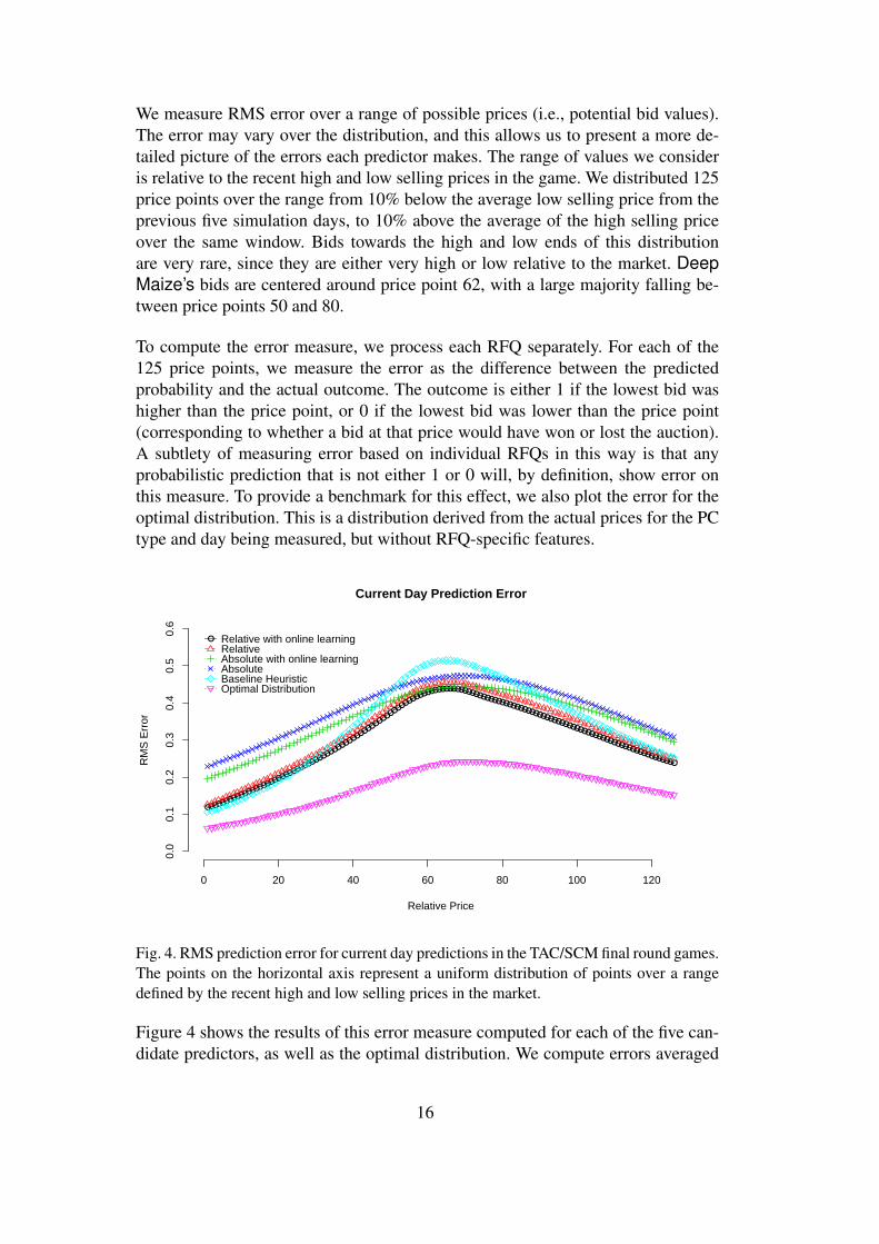
We measure RMS error over a range of possible prices (i.e., potential bid values).The error may vary over the distribution, and this allows us to present a more de-tailed picture of the errors each predictor makes. The range of values we consideris relative to the recent high and low selling prices in the game. We distributed 125price points over the range from 10% below the average low selling price from theprevious five simulation days, to 10% above the average of the high selling priceover the same window. Bids towards the high and low ends of this distributionare very rare, since they are either very high or low relative to the market. DeepMaize’s bids are centered around price point 62, with a large majority falling be-tween price points 50 and 80.

To compute the error measure, we process each RFQ separately. For each of the125 price points, we measure the error as the difference between the predictedprobability and the actual outcome. The outcome is either 1 if the lowest bid washigher than the price point, or 0 if the lowest bid was lower than the price point(corresponding to whether a bid at that price would have won or lost the auction).A subtlety of measuring error based on individual RFQs in this way is that anyprobabilistic prediction that is not either 1 or 0 will, by definition, show error onthis measure. To provide a benchmark for this effect, we also plot the error for theoptimal distribution. This is a distribution derived from the actual prices for the PCtype and day being measured, but without RFQ-specific features.

●●●●●●●●●●●●●●●●●●●●●●●●●●●●●●●●●●●●●●●●●●●●●●●●●●●●●●●●●●●●●●●●●●●●●●●●●●●●●●●●●●●●●●●●●●●●●●●●●●●●●●●●●●●●●●●●●●●●●●●●●●●●●●

0 20 40 60 80 100 120

0.0

0.1

0.2

0.3

0.4

0.5

0.6

Current Day Prediction Error

Relative Price

RM

S E

rror

● Relative with online learningRelativeAbsolute with online learningAbsoluteBaseline HeuristicOptimal Distribution

Fig. 4. RMS prediction error for current day predictions in the TAC/SCM final round games.The points on the horizontal axis represent a uniform distribution of points over a rangedefined by the recent high and low selling prices in the market.

Figure 4 shows the results of this error measure computed for each of the five can-didate predictors, as well as the optimal distribution. We compute errors averaged

16

over all games from the 2005 tournament final round, restricted to predictions madefor the middle part of the game from simulation day 20 to 200. This restriction isprimarily because the baseline predictor is not designed for border cases, such aswhen no recent price observations are available. The error of the baseline is artifi-cially high in these cases, which would distort the overall error results in favor ofour methods.

Of the candidate predictors, the relative predictor with online learning has the low-est overall prediction error. All four of our predictors have lower error than thebaseline in the center part of the distribution. The two absolute predictors havegreater error when making predictions for very high or very low prices. Onlinelearning reduces prediction error across the entire distribution for both the absoluteand relative representations. The relative predictors generally perform better thanthe absolute predictors. However, the absolute predictor with online learning haslower error than the relative predictor without online learning in the center of theprice distribution. This is where online learning should have the greatest impact,since more bids are placed in this region and it has more data to make updates. Thedifferences in error between our predictors and the baseline are quite substantial. Inthe center of the distribution, the difference between the baseline method and theoptimal method is approximately 0.3, and the difference between the optimal andthe relative predictor with online learning is approximately 0.2, an improvement ofroughly 30%.

Conceptually, errors towards the center of the distribution are likely to be muchmore important because bids are centered there. However, is not clear how errorsshould be weighted, since bid densities may vary in different situations (and cer-tainly for different agents). These predictions are also used for making non-biddingdecisions, which may use the information in different ways. Using supply-chainperformance (as we do in Section 5.2 below) is one way to resolve this dilemma,since we can test the predictors as they are used by a real decision-making proce-dure.

5.1.2 Future Forecasting Error

A distinctive feature of Deep Maize is that it explicitly forecasts changes in fu-ture market conditions. For future days, the agent translates its predictions into aneffective demand curve for use in production scheduling. This demand curve spec-ifies the price the agent would need to bid to win a particular quantity of PCs, onaverage. These prices are given in an ordered list, with the first price representingthe bid to win one PC, the second price the bid to win two PCs, and so on. Thepredictor gives the probability of winning a bid Pr(win|bid), which we combinewith the predicted overall demand to determine the expected quantity won for any

17

given bid level. Inverting this function yields the desired prices. 12

●

●

●

●

●

●

●

●

●●

0 10 20 30 40 50

0.00

0.05

0.10

0.15

0.20

Future Prediction Error

Prediction Horizon (days)

RM

S E

rror

● Relative with online learningRelativeAbsolute with online learningAbsoluteBaseline Heuristic

Fig. 5. RMS error between predicted and actual effective demand curves out to a horizonof 50 days, computed on the 2005 finals.

We measure the error for this effective demand curve, which combines errors fromthe price predictions and demand predictions. For each simulation day, we computethe actual demand curve by sorting the observed prices for each PC. We then mea-sure the RMS error between the prices in this list and the predicted demand curve,summing the errors for each PC in the list up to a maximum of 200 values perday. 13 Figure 5 compares the five predictors on this aggregate measure of futureforecasting error out to a prediction horizon of 50 days.

The pattern of results is similar to the results for the current day. The two relativepredictors score the best over all horizons, followed by the baseline and then thetwo absolute predictors. The online affine transformations are beneficial regardlessof the representation used. We note that this measure averages error over the dis-tribution (each data point represents a compression of the full distribution shownin Figure 4). We present information in this way partially for easy visualization,but also because future planning may be more dependent on errors over the entiredistribution than bidding decisions. However, we should note that the absolute pre-dictor shows higher overall error on this measure primarily because of errors at theextreme parts of the distribution, as in the short-term error results.

12 Our functional form allows simple inversion of this function, but this inversion can alsobe computed using a simple binary search to find the necessary bid level.13 An agent typically projects selling 100 or fewer PCs of any type on a given day, so thisis roughly twice the number of values the agent actually uses to make decisions.

18

5.2 Supply-Chain Performance

Since our forecasting methods were specifically designed to support decision mak-ing in a fully implemented and automated agent, we have the opportunity to assesshow forecasts impact agent performance. This is particularly interesting becauseof the complex interactions between prediction error and decisions. As discussedabove, it can be difficult to determine how to weight different types of predictionerrors. Another issue with online predictions is that the decisions made affect theinformation available for making future predictions.

We ran simulations using a profile of two MinneTAC-05 agents, two TacTex-05agents, one static version of Deep Maize, and one modified version. MinneTAC-05 and TacTex-05 were finalists in 2005 that were among the first to release agentbinaries. We ran four sets of games with a minimum of 35 samples. The staticversion of Deep Maize used the relative affine predictor. We present results asdifferences between the static and variable versions of Deep Maize. This pairingreduces variance but introduces bias to the extent that varying the sixth agent affectsthe performance of the static version. Another important caveat is that these resultsare for a single profile of strategies. More systematic approaches to selecting testenvironments may be better justified on game-theoretic grounds [17], but we makedo with a single convenient albeit ad hoc profile here.

In addition to scores we give three measures of customer sales performance: av-erage selling price (ASP), “selling efficiency”, and “timing efficiency”. Selling ef-ficiency is the fraction of achieved revenue to the maximum possible revenue foridentical daily sales, given perfect information about opponents’ bids and the optionto partially fill orders. Timing efficiency measures how well the agent distributedsales over time. Let the t-optimal same day selling price be the highest ASP theagent could achieve by selling each PC at most t days after it was actually deliv-ered and no earlier than it was actually produced. PCs are labeled according to aFIFO queuing policy. Timing efficiency is the ratio of the t-optimal same day sell-ing price to the selling efficiency. This factors out the effects of bidding policy andleaves the effects of deciding which days to sell on. The appeal of these additionalmetrics is that they allow us to compare a specific element of decision performanceagainst an optimal value, though we must remain cognizant of the additional con-straints when interpreting the results.

The simulation results are in Table 2. The most striking point is that all of ourkNN-based predictors comfortably outperform the same agent using the baselinepredictor. To calibrate, the difference between the top and bottom scores in the2005 finals was approximately 6.5 M, less than the advantage of any of our pre-dictors over the baseline. Clearly, effective prediction can have a sizable impact onagent performance when the decision-making architecture is capable of exploitingthe information. The affine transformations again showed benefits for both repre-

19

Predictor Score ASP Selling Efficiency 20-day Timing

Relative, No Affine –2.3M 0.004 –0.007 –0.015

Absolute, Affine 0.3M 0.001 –0.008 0.000

Absolute, No Affine –1.2M 0.007 –0.014 –0.009

Baseline –9.1M –0.032 0.002 –0.032Table 2Performance measures in simulated games. The numbers represent the difference betweentwo versions of Deep Maize using the relative affine predictor and the indicated predictor.

sentations.

The absolute predictors scored better than the relative predictors, albeit by fairlysmall margins. This is somewhat unexpected, given the error results. Earlier resultsusing a smaller data set for the predictors actually showed a slight advantage forthe relative predictor. We expect a larger data set to benefit the absolute represen-tation disproportionately because some of the features are based on current prices.With more data more similar instances are available, and the absolute represen-tation should predict more like the relative representation. We conjecture that therelative representation may have greater advantages for smaller data sets, but havenot verified this experimentally. Another likely explanation for this discrepancy isthat the absolute representation better reflects the actual uncertainty present be-cause it is able to spread predictions over a broader range of prices. This may causethe agent to delay making purchasing decisions until more information is available,potentially improving performance.

In general, the differences between the agent variations on the sales metrics are rel-atively small, but we note some interesting features. The timing measure correlatesquite well with the overall scores. The baseline predictor performs very poorly onthis measure as well as having a low ASP. The selling efficiency numbers do notshow a strong pattern, and the ASP numbers for the kNN variations are also am-biguous. This suggest that one of the more consistent benefits of better forecastsfor Deep Maize is the usefulness of these forecasts in timing sales activity.

5.3 Tournament and Self-Play Data

We also generated error scores for the four predictor variants using only the tourna-ment data set and only the self-play data set (a total of 12 different variations). Wedo not present full data here, but can describe the pattern of results fairly easily. Us-ing only the tournament data resulted in almost exactly equivalent performance tousing the combined data sets. The results using only the self-play data were almostalways worse than either the tournament only or combined settings. One conclu-sion we draw from this is that the process we used to generate the self-play data did

20

not produce the most relevant experience for making predictions. Another is thatthe online scoring procedure was effective at detecting the source of more salientinformation to use in the combined predictor. It does this by placing a very highvalue on the variable b in Eq. (4), weighting the tournament data set much moreheavily than the self-play data set. As the agent plays a game, we often observevalues set to the maximum possible value, within the range of allowable values.

6 Methods for Component Market Predictions

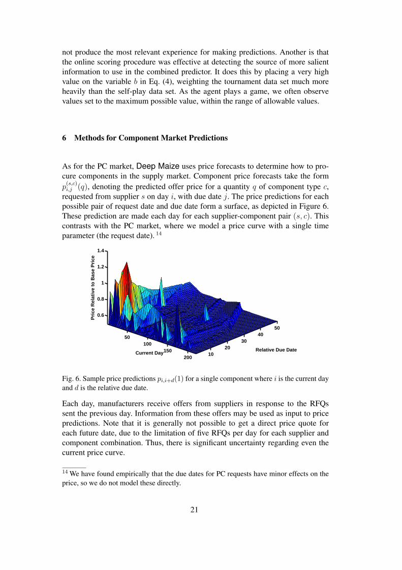
As for the PC market, Deep Maize uses price forecasts to determine how to pro-cure components in the supply market. Component price forecasts take the formp

(s,c)i,j (q), denoting the predicted offer price for a quantity q of component type c,

requested from supplier s on day i, with due date j. The price predictions for eachpossible pair of request date and due date form a surface, as depicted in Figure 6.These prediction are made each day for each supplier-component pair (s, c). Thiscontrasts with the PC market, where we model a price curve with a single timeparameter (the request date). 14

50100

150200

1020

3040

50

0.6

0.8

1

1.2

1.4

Relative Due Date

Supplier Price Prediction on Component 300

Current Day

Pri

ce R

elat

ive

to B

ase

Pri

ce

Fig. 6. Sample price predictions pi,i+d(1) for a single component where i is the current dayand d is the relative due date.

Each day, manufacturers receive offers from suppliers in response to the RFQssent the previous day. Information from these offers may be used as input to pricepredictions. Note that it is generally not possible to get a direct price quote foreach future date, due to the limitation of five RFQs per day for each supplier andcomponent combination. Thus, there is significant uncertainty regarding even thecurrent price curve.

14 We have found empirically that the due dates for PC requests have minor effects on theprice, so we do not model these directly.

21

We consider three classes of prediction methods for the component market. Thefirst creates an estimate of the current price curve using the observed spot pricequotes and linear interpolation. This method does not attempt to predict changesin prices over time. The second approach augments the first by using market indi-cators to predict residual changes from the estimated price curve over time. Thismethod exploits local price stability in the short term by using the linear interpola-tion model as a base, but still allows for modeling price variability over time. Thefinal method applies regression to predict prices directly based on market indica-tors. This method allows for the greatest flexibility in predicting price changes.

6.1 Linear Interpolation Price Predictor

As noted in many accounts of TAC/SCM agents, market prices in the game tend toexhibit local price stability over short horizons. The degree of volatility may varydepending on the particular agents playing and random variations in the underlyinggame state. However, there are structural reasons to expect such stability. One is thatthe underlying supplier capacity and customer demand levels change over time, butrarely exhibit drastic changes over short time periods. In addition, the outstandingcommitments and inventory of suppliers and manufacturers tend to exert a dampingeffect on component price changes.

Deep Maize estimates the current market state based on price quotes from recentdays. We employ linear interpolation to estimate prices for due dates with no recentobservations. Figure 7 shows an example price curve estimated using this method,which we term the linear interpolation price predictor (LIPP). Due to local pricestability, we expect LIPP to be a reasonably good predictor for prices in the nearfuture. Empirical results below support this proposition.

6.2 Relative Component Price Predictor

In analyzing the performance of LIPP, we note a tendency for predictions over theentire price curve to systematically overestimate or underestimate prices. There areseveral plausible reasons for this. Recall that suppliers’ current capacity varies ac-cording to a random walk during the game. Suppliers construct prices in part basedon projecting their current production capacity into the future to determine theiravailable capacity. Since available capacity is used in pricing for all request dates,fluctuations in capacity cause prices for all of these dates to rise or fall in unison.This pattern could also result from manufacturing agents increasing or decreasingorder quantities, but maintaining approximately the same timing in their purchaseschedules. This might result, for instance, from rising or falling customer demandlevels.

22

100 110 120 130 140

500

520

540

560

580

600

Day Due

Pric

e

Fig. 7. A sample linear interpolation of recent price quotes.

LIPP does not take into account any information beyond recent price quotes thatmight help to predict these sorts of price fluctuations. We introduce the relativecomponent price predictor (RCPP) as a way of exploiting these additional formsof information. RCPP predicts the residual error of LIPP by applying regressionto technical attributes summarizing the observable market state. A list of the at-tributes we used is given in Table 3. The predictions made by RCPP are formed bycalculating the summation of the residual errors and LIPP predictions.

The intuition for this approach is that the RCPP algorithm identifies game statesthat are likely to result in predictable price shifts, leading to inaccurate LIPP esti-mates. The residuals modify the current price estimates to account for these shifts.This approach exploits the short-term accuracy of the linear price predictor, whileexploiting historical data and market indicators to adapt future forecasts. We notethat there is a parallel between this approach and the relative representation used inpredicting prices in the PC market.

6.3 Absolute Component Price Predictor

The final class of predictors we consider is the absolute component price predictor(ACPP). ACPP applies regression to directly learn prices from the technical indi-cators. Unlike RCPP, this approach does not bootstrap the short-term accuracy ofLIPP, so it is not relative to the estimated current prices. The potential advantageof this approach is that it offers greater flexibility for modeling price shifts, sinceit is not constrained by the LIPP prediction. If there are prevailing long-term pricetrends not captured in the RCPP residuals, ACPP may yield more accurate predic-

23

tions at long horizons. We note that there is a parallel between this approach andthe absolute representation used in predicting prices in the PC market.

7 Evaluation of Component Market Predictions

We evaluate the relative performance of the three classes of predictors on the basisof prediction error using the Prediction Challenge framework. We present the re-sults of experiments run after the competition using the data set from the final roundof the 2007 Prediction Challenge. 15 The data consists of a total of 48 games con-taining the designated PAgent, divided into three sets of 16 games played againstthe same set of opponents. All opponents were selected from the agent repository.The predictors are scored using normalized RMS error on all required componentprice predictions.

7.1 Setting Expiration Intervals for LIPP

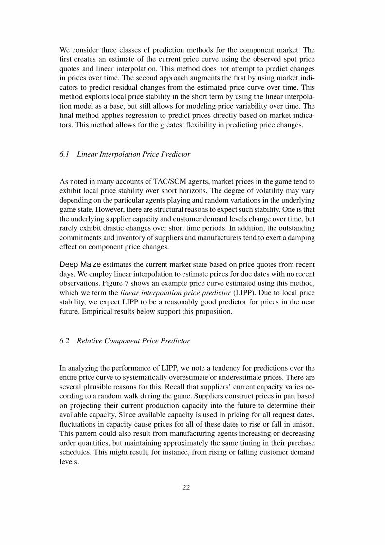
We begin by exploring an important parameter of the LIPP method, which we thenfix for subsequent analysis. Recall that manufacturers are limited in the numberof RFQs they may submit each day. We can increase the number of observationsavailable for estimating the price curve by including RFQ responses from previousdays, with the caveat that these quotes may represent stale information. We repre-sent this tradeoff using an expiration interval that determines how many days ofprevious observations are used to construct the LIPP estimate. Using a longer in-terval increases the amount of data available, along with the risk that the data nolonger accurately reflects the current situation. To determine the best setting of theexpiration interval, we tested intervals from one to five days. The results are shownin Figure 8.

The mean accuracy of the LIPP predictions decreases monotonically as the size ofthe length of the expiration interval is increased. This result implies that the day-to-day price volatility in TAC/SCM is high enough that the benefit of having datapoints for additional due dates is outweighed by the reduced accuracy of the olderdata points. It is possible that adapting this expiration interval dynamically during agame based on observed price volatility or other factors could yield more accuratepredictions, but we have not yet fully explored this possibility.

15 Many of these analyses were also performed before the Challenge using other test sets;we repeat all of the experiments using this data set for consistency

24

EX1 EX2 EX3 EX4 EX5

0.03

50.

040

0.04

50.

050

Expiration Interval

RM

S E

rror

Fig. 8. RMS error for LIPP with various expiration intervals.

7.2 Estimating Attribute Quality for Regression Models

As a preliminary step to regression, we seek to evaluate the quality of variousattributes that may be used to predict current and future component prices. Un-like classification problems, there are few measures of attribute quality availablefrom the current literature. For example, information gain, j-measure, and χ2 can-not be used for estimating attribute quality in a regression. Three measures thathave been proposed for regression with numerical attributes are mean absolute andmean squared error [4], and RReliefF [34]. Because the error measures assumeindependence among attributes, they are less appropriate given strong interdepen-dencies like those introduced in our analysis. In contrast, RReliefF has be shownempirically to perform well in situations where there are strong interdependencies,such as parity problems. A short explanation of the RReliefF values is rather elu-sive (see related work [35] for a thorough exposition), but we attempt here to givesome intuition as to what the values represent.

RReliefF is an extension of the ReliefF algorithm to regression. In classification,ReliefF measures an attribute’s quality according to how well a given attribute dis-tinguishes instances that are similar in the attribute space. The value itself is theapproximated difference of two probabilities with respect to a given attribute value.The first is the probability that a different value is observed given near instancesfrom different classes. The second is the probability that a different value is ob-served given near instances from the same class. Because price predictions and, ingeneral, regressions are continuous, we cannot calculate these probabilities. RReli-

25

efF attempts to solve this problem by introducing a probability distribution whichdetermines whether two instances are different. The values calculated by RReliefFlie in the range [−1, 1] with random attributes tending to be slightly negative. Atthe extremes, a value of near one signifies that a different attribute value impliesa different regression value for nearby instances. A RReliefF value greater thanzero indicates that the first probability subsumes the second and thus the attributeis likely to discriminate nearby instances to a useful extent. We adopt this simplethreshold to determine whether attributes are included in our regression models.Our experience is consistent with the empirical findings that RReliefF attribute se-lection improves our regression models over the default model that includes allavailable attributes.Table 3Attributes considered by RCPP and their RReliefF values for current and future days. Thefirst five attributes correspond to parameters of an individual RFQ and the remainder ofmarket state.

Attribute Current Future Description

day –0.000603 0.000842 current day

sent-day –0.000603 0.000842 day the RFQ will be sent

due-day 0.000124 0.001038 day the RFQ will be due

duration 0.000209 0.000603 due-day minus sent-day

quantity 0.011297 0.013593 RFQ quantity

linear-price 0.019816 0.010123 LIPP price prediction

nearest-price-point-diff –0.001689 –0.002899 nearest known price point distance (days from due date)

days-since-data –0.006886 0.006228 days since due date had a price quote

market-capacity –0.000496 0.00023 last supplier capacity from market report

estimated-capacity –0.000317 0.001029 estimate of supplier capacity using market reports and trend

surplus –0.000514 0.000157 available capacity minus agent demand in recent period

aggregate-surplus –0.000618 0.000295 available capacity minus agent demand in total

mean-demand –0.001663 0.000741 mean customer demand for component

mean-low-demand –0.002198 0.001023 mean customer demand for low-end components

mean-mid-demand –0.0014 0.0009 mean customer demand for mid-range components

mean-high-demand –0.002 –0.000787 mean customer demand for high-end components

5-day-demand –0.001258 0.000852 customer demand for last 5 days

20-day-demand –0.000687 0.00164 customer demand for last 20 days

40-day-demand –0.000833 0.0014 customer demand for last 40 days

A complete list of all attributes considered for regression analysis as well as theRReliefF values for each attribute on both current and future day predictions isgiven in Table 3. The attributes are a mix of RFQ parameters and estimated marketstate. Note that RReliefF values often differ significantly with respect to currentand future predictions. In particular, the table suggests that current predictions arebest determined by the attribute subset quantity, due-day, duration, and linear-price,all but the last of which are RFQ parameter attributes. This differs notably fromfuture predictions , for which the majority of attributes are still of threshold quality.Component prices vary loosely according to a few market state parameters that

26

are hidden from direct observation. Our attribute set was chosen in an attempt toextract useful observable parameters from the market in lieu of the hidden state. Forcurrent predictions, it appears that the market state attributes are not very useful inregression. This is likely explained by the observation that the internal market statechanges gradually and that useful portions of the internal state are already expressedin the LIPP prices from the prior day. Thus, current prices can best be determinedby attributes from the RFQ and LIPP prices, whereas including the estimates ofmarket state is not beneficial. This is not to say that estimating internal marketstate is without predictive power in all cases. As the RRefliefF values in the futurecolumn suggest, the future market state is no longer reflected in LIPP prices andincluding these attributes is likely beneficial.

7.3 Comparing Regression Methods for RCPP

There are many machine learning algorithms that could be applied to learn theresidual errors for RCPP. We tested a variety of regression algorithms from theWeka machine learning package [39] for this task, including linear regression,kNN, support vector machines, and various decision-tree regressions. We gener-ated training data from approximately 50 game instances simulated on a local com-puting cluster. Each game of training data had one PAgent playing, along with acollection of other agents taken from the agent repository (the same set of potentialopponents used for the Prediction Challenge). Each game contains approximately1800 sample price predictions for each CPU component and twice as many fornon-CPU components. We train separate predictors for each component type, sowe have approximately 90,000 data points for CPU components and 180,000 fornon-CPU components. We take samples from the viewpoint of the PAgent in thetraining games, so the market indicators are computed with respect to this agent’sobservations.

After some preliminary experimentation, we selected additive regression 16 andreduced-error pruning trees (REP trees) as the most promising candidates. Manyof the other algorithms had similar results in terms of prediction error, but requiredmuch longer to train or generated very large models. For some of the algorithms,overfitting was a severe problem. We tested several parameter settings for bothadditive regression and REP trees using the data set from the final round of thePrediction Challenge. Additive regression was tested both with default settings andwith a shrinkage rate of 10%. 17 REP Trees were tested with maximum tree depths

16 Additive regression is a meta-learning algorithm wherein each decision stump is fit tothe residual of the previous step every iteration.17 The shrinkage rate considers how much of the trained decision stump is used each itera-tion. Normally, the shrinkage rate is set to 100%, however, a smaller shrinkage rate inducesa smoothing effect and reduces overfitting.

27

of four through seven. All variations learned residuals from LIPP predictions withan expiration interval of one (the best setting from the previous section).

AddReg Shrink REP4 REP5 REP6 REP7

0.03

50.

040

0.04

50.

050

Predictor

Cur

rent

RM

S E

rror

AddReg Shrink REP4 REP5 REP6 REP7

0.08

0.09

0.10

0.11

Predictor

Fut

ure

RM

S E

rror

Fig. 9. Prediction error results for various candidate learning algorithms on the data setfrom the final round of the Prediction Challenge. Future corresponds to a 20-day horizon.

Figure 9 shows the prediction error results for these methods on both current andfuture predictions. The different learning algorithms produced very similar results;each would have placed first in both component prediction categories. For the ac-tual Challenge, we used the REP tree algorithm with maximum depth five to learnresiduals for RCPP, since this algorithm was consistently accurate for both currentand future predictions.

7.4 Comparison of Prediction Methods

In the previous sections, we explored variations of the LIPP and RCPP methods toidentify good parameter settings for these algorithms. We now directly compare theperformance of the three different classes of methods introduced in Section 6. Weuse the LIPP method with expiration interval one, the RCPP method learning resid-uals using REP trees of max depth five, and an ACPP predictor that uses additiveregression to make price predictions directly from the technical indicators. 18 Pre-diction error results for all three algorithms on both current and future predictionsare given in Figure 10. All current comparisons in the figure are statistically signifi-cant beyond the 0.005 level and all future comparisons in the figure are statisticallysignificant beyond the 0.05 level using a standard t-test.

For the current price predictions, the performance for LIPP and RCPP is very close,with both outperforming the absolute predictor by a wide margin. This is strongevidence that the LIPP method effectively summarizes the current price state, and

18 Based on the results in the previous section, we would expect a REP-tree version ofACPP to have very similar performance.

28

ACPP RCPP LIPP

0.03

50.

045

0.05

5

Predictor

Cur

rent

RM

S E

rror

ACPP RCPP LIPP

0.08

0.09

0.10

0.11

0.12

Predictor

Fut

ure

RM

S E

rror

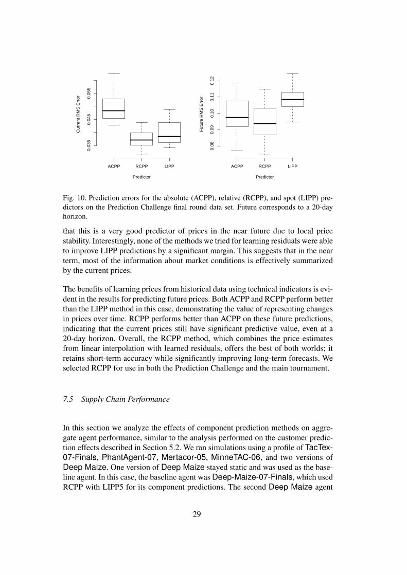
Fig. 10. Prediction errors for the absolute (ACPP), relative (RCPP), and spot (LIPP) pre-dictors on the Prediction Challenge final round data set. Future corresponds to a 20-dayhorizon.

that this is a very good predictor of prices in the near future due to local pricestability. Interestingly, none of the methods we tried for learning residuals were ableto improve LIPP predictions by a significant margin. This suggests that in the nearterm, most of the information about market conditions is effectively summarizedby the current prices.

The benefits of learning prices from historical data using technical indicators is evi-dent in the results for predicting future prices. Both ACPP and RCPP perform betterthan the LIPP method in this case, demonstrating the value of representing changesin prices over time. RCPP performs better than ACPP on these future predictions,indicating that the current prices still have significant predictive value, even at a20-day horizon. Overall, the RCPP method, which combines the price estimatesfrom linear interpolation with learned residuals, offers the best of both worlds; itretains short-term accuracy while significantly improving long-term forecasts. Weselected RCPP for use in both the Prediction Challenge and the main tournament.

7.5 Supply Chain Performance

In this section we analyze the effects of component prediction methods on aggre-gate agent performance, similar to the analysis performed on the customer predic-tion effects described in Section 5.2. We ran simulations using a profile of TacTex-07-Finals, PhantAgent-07, Mertacor-05, MinneTAC-06, and two versions ofDeep Maize. One version of Deep Maize stayed static and was used as the base-line agent. In this case, the baseline agent was Deep-Maize-07-Finals, which usedRCPP with LIPP5 for its component predictions. The second Deep Maize agent

29

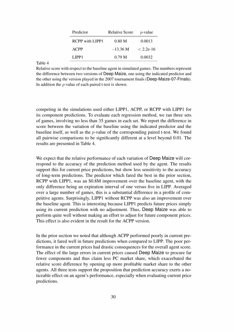
Predictor Relative Score p-value

RCPP with LIPP1 0.80 M 0.0013

ACPP –13.36 M < 2.2e-16

LIPP1 0.79 M 0.0032Table 4Relative score with respect to the baseline agent in simulated games. The numbers representthe difference between two versions of Deep Maize, one using the indicated predictor andthe other using the version played in the 2007 tournament finals (Deep-Maize-07-Finals).In addition the p-value of each paired t-test is shown.

competing in the simulations used either LIPP1, ACPP, or RCPP with LIPP1 forits component predictions. To evaluate each regression method, we ran three setsof games, involving no less than 35 games in each set. We report the difference inscore between the variation of the baseline using the indicated predictor and thebaseline itself, as well as the p-value of the corresponding paired t-test. We foundall pairwise comparisons to be significantly different at a level beyond 0.01. Theresults are presented in Table 4.

We expect that the relative performance of each variation of Deep Maize will cor-respond to the accuracy of the prediction method used by the agent. The resultssupport this for current price predictions, but show less sensitivity to the accuracyof long-term predictions. The predictor which fared the best in the prior section,RCPP with LIPP1, was an $0.8M improvement over the baseline agent, with theonly difference being an expiration interval of one versus five in LIPP. Averagedover a large number of games, this is a substantial difference in a profile of com-petitive agents. Surprisingly, LIPP1 without RCPP was also an improvement overthe baseline agent. This is interesting because LIPP1 predicts future prices simplyusing its current prediction with no adjustment. Thus, Deep Maize was able toperform quite well without making an effort to adjust for future component prices.This effect is also evident in the result for the ACPP version.

In the prior section we noted that although ACPP performed poorly in current pre-dictions, it fared well in future predictions when compared to LIPP. The poor per-formance in the current prices had drastic consequences for the overall agent score.The effect of the large errors in current prices caused Deep Maize to procure farfewer components and thus claim less PC market share, which exacerbated therelative score difference by opening up more profitable market share to the otheragents. All three tests support the proposition that prediction accuracy exerts a no-ticeable effect on an agent’s performance, especially when evaluating current pricepredictions.

30

8 TAC/SCM Tournament and Prediction Challenge

The TAC/SCM tournament and Prediction Challenge offer distinct opportunities forevaluation of our prediction methods in comparison with alternatives outside ourcontrol. The Prediction Challenge facilitates direct comparisons with competingprediction approaches, isolating this aspect of the game. The general tournamentresults allow us to evaluate the general competency of our agent relative to the othercompetitors. Predictions are an important component of Deep Maize’s decisionmaking, so the overall performance of the agent reflects in part the quality of thesepredictions. An important aspect of both the SCM tournament and the PredictionChallenge is that each new game instance may present novel strategic environmentsnot be reflected in any historical data. Thus, this exercise serves as an importantindication of the robustness of our prediction results.

8.1 TAC/SCM Tournaments

Tournament performance is an important indicator of the overall competence ofTAC/SCM agents. Each TAC/SCM tournament comprises a sequence of rounds:qualifying, seeding, quarter-finals, semi-finals, and finals. The qualifying and seed-ing rounds span several days and are used primarily for development and testing.The quarter-finals, semi-finals, and finals are held on successive days. In 2005 and2006, 24 agents were selected to begin the quarter-finals, with half eliminated ineach round. In 2007, 18 agents started the quarter-finals, with six eliminated ineach round. Results from the 2005, 2006, and 2007 tournament semi-final and finalrounds including Deep Maize are presented in Tables 5, 6, and 7. 19

Deep Maize has performed very well in each of the TAC/SCM tournaments todate. Our agent reached the final round each year, placing fourth in 2005, third in2006, and third in 2007. Deep Maize also demonstrated strong performance inthe semi-final rounds, placing first in each heat. This record of overall performanceprovides evidence that Deep Maize is effective in a wide variety of competitiveenvironments. The version of the customer prediction module presented here isvery similar to the modules that played in all the 2005–2007 tournaments. Thisaspect of the agent was largely unmodified between 2005 and 2007, though otherelements of the agent underwent significant revisions.

In 2005 and 2006, Deep Maize used only LIPP5 for component market predic-tions. RCPP was added to the predictions for the 2007 tournament (using a REPTree with a maximum depth five), however we still maintained an expiration in-terval of five for LIPP. Unfortunately, we did not discover the superior accuracy

19 More details about the tournament structure and full results are available at the TAC website, http://www.sics.se/tac.

31

Table 5Scores and rankings from the rounds Deep Maize played in during the 2005 SCM tour-nament. All scores are in millions of dollars. The adjusted column eliminates two gameinstances (3718 and 4259) where the University of Michigan network lost connectivityduring the game, distorting the results substantially.

Semi-Finals 2 Finals Finals (adjusted)

Deep Maize 3.68 TacTex-05 4.74 TacTex-05 5.18

TacTex-05 3.57 SouthamptonSCM 1.60 Deep Maize 2.06

MinneTAC 2.27 Mertacor 0.55 SouthamptonSCM 1.55

RationalSCM –2.28 Deep Maize –0.22 Mertacor 0.53

CMieux –2.33 MinneTAC –0.31 MinneTAC 0.33

PhantAgent –6.64 Maxon –1.99 Maxon –1.74

Table 6Scores and rankings from the rounds Deep Maize played in during the 2006 SCM tourna-ment. All scores are in millions of dollars.

Semi-Finals 2 Finals

Deep Maize 6.45 TacTex-06 5.85

Maxon 4.08 PhantAgent 4.15

Botticelli 1.95 Deep Maize 3.58

CMieux 1.81 Maxon 1.75

SouthamptonSCM 1.63 Botticelli 0.48

Mertacor 1.44 MinneTAC –2.70

Table 7Scores and rankings from the rounds Deep Maize played in during the 2007 SCM tourna-ment. All scores are in millions of dollars.

Semi-Finals 1 Finals

Deep Maize 9.76 PhantAgent 8.67

Tinhorn 6.94 TacTex 6.31

Maxon 5.63 DeepMaize 5.45

MasterBham 5.40 Maxon 1.79

CrocodileAgent 5.12 Tinhorn 1.34

Sorter95 –2.65 CMieux 1.24

32

of lower expiration intervals until shortly before the finals, such that we could notmake the modification and completely test the strategy. The training data used for2007 tournament play was derived from approximately 100 game instances, includ-ing games from the late rounds of the 2006 tournament and additional simulationsusing the best available agents from the agent repository.

8.2 TAC/SCM 2007 Prediction Challenge

The introduction of the Prediction Challenge allows us to directly compare ourprediction approaches to other competitors, supplementing our own analysis basedon controlled experiments. The Prediction Challenge was played in two rounds, asemi-final and a final. The semi-final round took place during the same time-frameas the TAC/SCM seeding round, before the main tournament. Like the qualifiersand seeding rounds in the main TAC/SCM tournament, this round was meant asa preliminary test of the overall Prediction Challenge for both the organizers andcompetitors. The final round took place the day before the main TAC/SCM finals.In both rounds, every competitor was given eight hours to make predictions aboutthe 48 games defining the round. Competitors were allowed to produce their pre-dictions any time during this period, independently of the other competitors.

The results from the Challenge semi-finals and finals are shown in Table 8. DeepMaize placed first overall in the finals, achieving the top score in both componentprediction categories and the second-best scores in both PC prediction categories.These results provide additional support for the overall efficacy of our methods.Deep Maize used a variation of RCPP for the semi-final round of the PredictionChallenge. Among other differences, this version used an expiration interval offive for the linear price interpolations. The final round version used an expirationinterval of one, which largely account for the significant improvement in currentcomponent price predictions between the semi-final and final round. The data setfor component price predictions was based on games specifically simulated for thePrediction Challenge, as discussed in Section 7.3. The customer price predictorused in the Challenge was identical to the version used by Deep Maize in the2006 TAC/SCM tournament, including the data set.

9 Conclusions

We document and analyze successful approaches for forecasting prices in a chal-lenging market domain. The general principle of our design is to support exploita-tion of all possible sources of information. To this end, we integrate several well-known ideas in an novel way, resulting in better overall predictions.

33

Table 8TAC/SCM Prediction Challenge 2007 Results (RMS error normalized by base price).

Prediction Agent Semi-Finals Finals

Current PCs

TacTex 0.04812 0.04554

Deep Maize 0.04632 0.04682

Botticelli 0.09449 0.04714

Kshitij 0.04882 0.04873

Future PCs

TacTex 0.09318 0.09156

Deep Maize 0.09473 0.09586

Botticelli 0.13984 0.10238

Kshitij 0.15428 0.11094

Current Components

Deep Maize 0.04810 0.03919

Botticelli 0.04163 0.04168

TacTex 0.04239 0.04284

Kshitij 0.10654 0.13333

Future Components

Deep Maize 0.09925 0.09427

Botticelli 0.10067 0.09700

TacTex 0.10714 0.10338

Kshitij 0.16324 0.13886

In the PC market we evaluate our ideas against a baseline predictor similar to thoseused by many competing agents, applying both error measures and simulation per-formance as benchmarks. We show that improved predictions can dramatically im-prove agent performance in TAC/SCM. This is particularly interesting in light ofthe substantial uncertainties inherent in the domain and challenges of predicting thebehavior of other agents.

The technique we present for applying transformations to predictions using onlinescoring is particularly interesting, and should be applicable in many domains. Thismethod provides a way to perform principled combinations of predictions based ondifferent sources of data, as well as a way to reduce systematic errors. It does theseby making use of additional information derived from online performance. Thismethod showed consistent benefits in our experiments across a range of conditionson both prediction error and simulation performance metrics.

We also investigated the use of absolute and relative representations for predic-tions. It appears that each of these representations has advantages under certainconditions, particularly related to how the information is used in decision making.

34

In the component market we develop methods to integrate volatile spot price predic-tions with a long term predictor using multiple sources of inter-market information.This relative predictor is more accurate than either the spot predictions or absoluteprice predictions from historical data in isolation.

Our prediction methods for both markets demonstrate strong overall performance,demonstrated in internal experiments and in our first-place finish in the inauguralTAC/SCM Prediction Challenge. These predictions have also contributed to thestrong overall performance of Deep Maize in the TAC/SCM tournament in recentyears.

Acknowledgments

Thanks to the participants and organizers of the TAC/SCM competition for pro-viding such a fruitful research environment. We owe particular gratitude to DavidPardoe for designing and operating the Prediction Challenge. Kevin O’Malley con-tributed to the Deep Maize infrastructure. This work was supported in part by NSFgrant IIS-0205435, and the STIET program under NSF IGERT grant 0114368.

References

[1] J. M. Bates and C. W. J. Granger. The combination of forecasts. Operations Research,20(4):451–468, 1969.

[2] M. Benisch, A. Greenwald, V. Naroditskiy, and M. Tschantz. A stochasticprogramming approach to scheduling in TAC SCM. In Fifth ACM Conference onElectronic Commerce, pages 152–159, New York, 2004.

[3] M. Benisch, A. Sardinha, J. Andrews, and N. Sadeh. CMieux: Adaptive strategies forcompetitive supply chain trading. In Eighth International Conference on ElectronicCommerce, pages 47–58, Ann Arbor, 2006.

[4] L. Breiman, J. Friedman, C. J. Stone, and R. Olshen. Classification and RegressionTrees. Chapman & Hall/CRC, 1984.

[5] P. J. Brockwell and R. A. Davis. Introduction to Time Series and Forecasting.Springer-Verlag, 1996.

[6] C. H. Brooks, R. Gazzale, R. Das, J. O. Kephart, J. K. MacKie-Mason, and E. H.Durfee. Model selection in an information economy: Choosing what to learn.Computational intelligence, 2002.

[7] D. A. Burke, K. N. Brown, B. Hnich, and A. Tarim. Learning market prices for a real-time supply chain management trading agent. In AAMAS-06 Workshop on TradingAgent Design and Analysis, Hakodate, 2006.

35

[8] C. Chatfield. Time-Series Forecasting. Chapman & Hall/CRC, 2001.

[9] S.-F. Cheng, E. Leung, K. M. Lochner, K. O’Malley, D. M. Reeves, and M. P.Wellman. Walverine: A Walrasian trading agent. Decision Support Systems, 39:169–184, 2005.

[10] R. T. Clemen and R. L. Winkler. Combining probability distributions from experts inrisk analysis. Risk Analysis, 19(2):187–203, 1999.

[11] J. Collins, R. Arunachalam, N. Sadeh, J. Eriksson, N. Finne, and S. Janson. Thesupply chain management game for the 2007 trading agent competition. TechnicalReport CMU-ISRI-07-100, Carnegie Mellon University, 2007.

[12] J. Eriksson, N. Finne, and S. Janson. Evolution of a supply chain management gamefor the Trading Agent Competition. AI Communications, 9:1–12, 2006.

[13] R. Ghani. Price prediction and insurance for online auctions. In InternationalConference on Knowledge Discovery in Data Mining, pages 411–418, 2005.

[14] R. Hanson. Combinatorial information market design. Information Systems Frontiers,5(1):107–119, 2003.

[15] T. Hastie, R. Tibshirani, and J. Friedman. Elements of Statistical Learning. Springer-Verlag, 2001.

[16] M. He, A. Rogers, X. Luo, and N. R. Jennings. Designing a successful trading agentfor supply chain management. In Fifth International Joint Conference on AutonomousAgents and Multiagent Systems, pages 1159–1166, Hakodate, 2006.

[17] P. R. Jordan, C. Kiekintveld, and M. P. Wellman. Empirical game-theoretic analysisof the TAC supply chain game. Sixth International Joint Conference on AutonomousAgents and Multiagent Systems, pages 1188–1195, 2007.

[18] P. J. Kaufman. Trading Systems and Methods. John Wiley and Sons, third edition,1998.

[19] P. W. Keller, F.-O. Duguay, and D. Precup. RedAgent-2003: An autonomousmarket-based supply-chain management agent. In Third International Conference onAutonomous Agents and Multiagent Systems, pages 1182–1189, 2004.

[20] W. Ketter. Identification and Prediction of Economic Regimes to Guide DecisionMaking in Multi-Agent Marketplaces. PhD thesis, University of Minnesota, January2007.

[21] W. Ketter, J. Collins, M. L. Gini, A. Gupta, and P. Schrater. A predictive empiricalmodel for pricing and resource allocation decisions. In Ninth International Conferenceon Electronic Commerce, pages 449–458, Minneapolis, 2007.

[22] C. Kiekintveld, J. Miller, P. R. Jordan, and M. P. Wellman. Controlling a supply chainagent using value-based decomposition. In Seventh ACM Conference on ElectronicCommerce, pages 208–217, Ann Arbor, 2006.

36

[23] C. Kiekintveld, J. Miller, P. R. Jordan, and M. P. Wellman. Forecasting market pricesin a supply chain game. In Sixth International Joint Conference on Autonomous Agentsand Multiagent Systems, pages 1318–1325, 2007.

[24] C. Kiekintveld, Y. Vorobeychik, and M. P. Wellman. An analysis of the 2004 supplychain management trading agent competition. In IJCAI-05 Workshop on TradingAgent Design and Analysis, Edinburgh, 2005.

[25] C. Kiekintveld, M. P. Wellman, S. Singh, J. Estelle, Y. Vorobeychik, V. Soni, andM. Rudary. Distributed feedback control for decision making on supply chains. InFourteenth International Conference on Automated Planning and Scheduling, pages384–392, Whistler, BC, 2004.

[26] F. J. Nogales, J. Contreras, A. J. Conejo, and R. Espinola. Forecasting next-dayelectricity prices by time series models. IEEE Transactions on Power Systems,17:342–348, 2002.

[27] A. Osepayshvili, M. P. Wellman, D. M. Reeves, and J. K. MacKie-Mason. Self-confirming price prediction for bidding in simultaneous ascending auctions. In Twenty-First Conference on Uncertainty in Artificial Intelligence, pages 441–449, Edinburgh,2005.

[28] D. Pardoe. The TAC SCM Prediction Challenge. http://www.cs.utexas.edu/˜TacTex/PredictionChallenge/, June 2007.

[29] D. Pardoe and P. Stone. Bidding for customer orders in TAC SCM. In Agent MediatedElectronic Commerce VI, volume 3435 of Lecture Notes in Artificial Intelligence.Springer, 2005.

[30] D. Pardoe and P. Stone. TacTex-05: A champion supply chain management agent.In Twenty-First National Conference on Artificial Intelligence, pages 1489–1494,Boston, 2006.

[31] D. Pardoe and P. Stone. Adapting price predictions in TAC SCM. In AAMAS-07Workshop on Agent Mediated Electronic Commerce IX, Honolulu, 2007.

[32] D. Pardoe and P. Stone. An autonomous agent for supply chain management. InG. Adomavicius and A. Gupta, editors, Handbooks in Information Systems Series:Business Computing. Elsevier, 2007.

[33] R. S. Pindyck and D. L. Rubinfeld. Econometric Models and Econometric Forecasts.Irwin/McGraw-Hill, 4th edition, 1998.

[34] M. Robnik-Sikonja and I. Kononenko. An adaptation of Relief for attribute estimationin regression. In Fourteenth International Conference on Machine Learning, pages296–304, Nashville, 1997.

[35] M. Robnik-Sikonja and I. Kononenko. Theoretical and empirical analysis of ReliefFand RReliefF. Machine Learning, 53:23–69, 2003.

[36] P. Stone, R. E. Schapire, M. L. Littman, J. A. Csirik, and D. McAllester. Decision-theoretic bidding based on learned density models in simultaneous, interactingauctions. Journal of Artificial Intelligence Research, 19:209–242, 2003.

37

[37] M. P. Wellman, A. Greenwald, and P. Stone. Autonomous Bidding Agents: Strategiesand Lessons from the Trading Agent Competition. MIT Press, 2007.

[38] M. P. Wellman, D. M. Reeves, K. M. Lochner, and Y. Vorobeychik. Price predictionin a trading agent competition. Journal of Artificial Intelligence Research, 21:19–36,2004.

[39] I. H. Witten and E. Frank. Data Mining: Practical Machine Learning Tools andTechniques with Java Implementations. Morgan Kaufmann, 2005.

38