Energy Conversion and Management 75 (2013) 561–569

Contents lists available at SciVerse ScienceDirect

Energy Conversion and Management

journal homepage: www.elsevier .com/ locate /enconman

Forecasting hourly global solar radiation using hybrid k-meansand nonlinear autoregressive neural network models

0196-8904/$ - see front matter � 2013 Elsevier Ltd. All rights reserved.http://dx.doi.org/10.1016/j.enconman.2013.07.003

⇑ Corresponding author. Tel.: +213 (0)29 93 21 17; fax: +213 (0)29 93 26 98.E-mail addresses: benkhalil3@gmail.com (K. Benmouiza), cheknanali@yahoo.

com, a.cheknane@mail.lagh-univ.dz (A. Cheknane).1 Tel.: +213 (0)778 73 85 56.

Khalil Benmouiza a,1, Ali Cheknane b,⇑a Département de Physique, Faculté des Sciences, Université Abou-Beker Belkaid de Tlemcen, BP 119, Tlemcen 13000, Algerieb Laboratoire des Semiconducteurs et Matériaux Fonctionnels, Université Amar Telidji de Laghouat, Algérie, BP 37G, Laghouat 03000, Algerie

a r t i c l e i n f o a b s t r a c t

Article history:Received 14 May 2013Accepted 5 July 2013

Keywords:Forecasting solar radiationArtificial neural networksClusteringPhase space reconstitution

In this paper, we review our work for forecasting hourly global horizontal solar radiation based on thecombination of unsupervised k-means clustering algorithm and artificial neural networks (ANN).k-Means algorithm focused on extracting useful information from the data with the aim of modelingthe time series behavior and find patterns of the input space by clustering the data. On the other hand,nonlinear autoregressive (NAR) neural networks are powerful computational models for modeling andforecasting nonlinear time series. Taking the advantage of both methods, a new method was proposedcombining k-means algorithm and NAR network to provide better forecasting results.

� 2013 Elsevier Ltd. All rights reserved.

1. Introduction solar radiation time series [36]. Moreover, global solar radiation

The generation of the energy in our modern industrialized soci-ety is still mainly based on a very limited resource. Some projec-tions show that the global energy demands will almost triple by2050 [10]. Thus, the search for alternative energy resources has be-come an important issue for our time. Solar energy is becoming avery attractive solution since it is considered an essentially inex-haustible and broadly available energy.

For an efficient conversion and utilization of solar power, solarradiation data should be measured continuously and accuratelyover the long-term. However, the measurement of solar radiationis not available for all countries in the world due to some technicaland fiscal limitations. Hence, several studies were proposed in theliterature to find mathematical and physical models to estimateand forecast the amount of solar radiations such as stochastic pre-diction models based on time series methods [14,36,39,40] andartificial neural network approaches [11,2,4].

Classical linear time series models like autoregressive movingaverage modeling [3] have been widely used in modeling of lineartime series [36]. Even so, it was proven that they are inadequate inthe analysis and prediction of solar radiation due to the non-stationary and nonlinearity of the solar radiation time series, espe-cially for cloudy sky [39,1,36]. In addition, stochastic models arebased on the probability estimation that needs a full identificationof the mathematical function, leads to a difficult forecasting of the

time series is a dynamical system that depends on some meteoro-logical elements such as temperature, water vapor, suspend solids,cloud and water air condition that can represent nonlinear charac-teristics [36,12,38] .

To overcome this problem, nonlinear approaches, such as artifi-cial neural networks (ANN) was considered a powerful tool forforecasting similar time series [39,28,36]. The advantages of theANN that it does not require the knowledge of the internal systemparameters that offer a compact solution for multiple variableproblems [11,2,36,4]. However, single models presented a big fore-casting error [36]. Thus, hybrid methods combining different mod-els have been widely used in the literature to improve the forecastperformance [36,12,5]. Nevertheless, no one of those methods willbe capable of presenting information about the behavior of the so-lar radiation time series in the future. Hence, it was used the TimeSeries Data Mining (TSDM) methodology [33] which is a funda-mental contribution to the fields of time series analysis and datamining that allows a search, for valuable information on nonlinearproblems such as solar radiation time series [21].

Data mining is the identification of interesting structure in thedata, where the structure designates patterns of the data and rela-tionships among regions of the data; it is a process of groupingsimilar elements gathered closely using unsupervised clusteringmethods such as k-means and c-means algorithms [37]. Data min-ing techniques were used in a wide variety of fields for prediction.For example, in stock prices, meteorological data, customer behav-ior, production control and other types of scientific data [9].

Taking the two advantages of both methods, the k-means ap-proach [25] for clustering the solar radiation data to extract useful

562 K. Benmouiza, A. Cheknane / Energy Conversion and Management 75 (2013) 561–569

information and the ANN for forecasting purposes, a new methodwas proposed in this paper that combines an unsupervised k-means clustering algorithm and nonlinear autoregressive neuralnetwork.

At the first stage, the data obtained from the phase space recon-stitution using Takens theorem [35] were clustered using k-meanalgorithm; clustering is a process of grouping an unlabelled set ofexamples into several clusters such that a similar pattern is associ-ated with every cluster. The motivation of using the k-meansapproach in this paper is due to its simplicity and also to the factthat the proposed methods do not require an advanced clusteringalgorithm. However, one of the vital issues of the k-means algo-rithm is the choosing of the appropriate number of clusters [37].Therefore, a silhouette function proposed by [32,23] was used toobtain the best number of bunches.

At the second stage, the nonlinear autoregressive (NAR) neuralnetwork that is a multilayer perceptron neural network (MLP) withsome modification was applied for forecasting the solar radiationtime series trying different architecture to get the best networkstructure. Combining those two methods presented better resultsfor multi-step ahead prediction in long term forecasting.

The remaining part of this paper is organized as follows. Section2 presented the methodology used in this work for forecasting thesolar radiation time series using time series data mining technique,a background of space phase reconstitution, k-means clusteringalgorithm and NAR network methods were also viewed. In Section3, we simulated the forecasting results of the proposed method andcomparing the results with the measured ones. The last sectionwas devoted to the conclusion and discussion of future works.

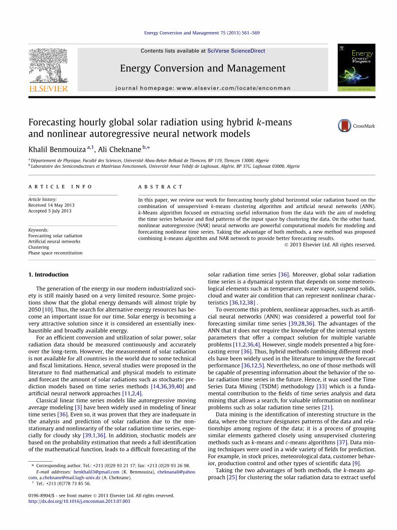
2. Methodology

A time series is a collection of time ordered observations x(ti),each one being entered at a specific time t called a period [30].

Fig. 1. The proposed methodology for t

Modeling and forecasting of the time series are an importation taskto extract useful information from the data [7]. Hence, in this pa-per, a proposed method that relies on principles of time seriesanalysis, unsupervised clustering, artificial neural networks andevolutionary optimization methods were proposed as presentedin Fig. 1. The methodology can be outlined in the following steps:

(1) Determine the minimum, appropriate, embedding dimen-sion for phase space reconstruction for the time series [15];

(2) Identify regions of the reconstructed phase-space which hassimilar characteristics using k-means clustering algorithm;

(3) For each cluster train different NAR neural network to gener-ate regional predictor for forecasting local regions;

(4) Use the corresponding NAR neural network using differentdelay and neurons to generate a global prediction for thetime series;

(5) Reconstructed phase-space of the obtained time series fromstep 4, then use the appropriate k-means method to clusterthe data using the same parameters used in step 1 and step2;

(6) To perform the forecast, assign each pattern from step 5 tothe appropriate region obtained from step 3 using as a crite-rion the Euclidean distance:- If the Euclidean distance between each region and theassigned pattern is small, then it was considered a betterforecast, else return to step 4.

2.1. Determining an appropriate embedding dimension

Phase space reconstruction provides a simplified, multidimen-sional representation of a nonlinear time series that simplifies fur-ther analysis. The approach of phase-space reconstruction consistsof embedding the time series into a higher-dimensional space tosee the underlying dynamical system [15]. The most widely usedversion of embedding is a time delay embedding [35]. This method

ime series data mining forecasting.

K. Benmouiza, A. Cheknane / Energy Conversion and Management 75 (2013) 561–569 563

embeds a scalar time series x(ti) into a m-dimensional space de-noted X(ti), as expressed in the following equation,

XðtiÞ ¼ ðxðtiÞ; xðti þ sÞ; � � � ; xðti þ ðm� 1ÞsÞ ð1Þ

where i ¼ ð1;2; . . . ;MÞ, s is the delay time, m is the embeddingdimension, and M is the number of embedded points in them-dimensional space given by Eq. (2). N is the total number ofpoints of the time series and XðtiÞ is the embedded time series intoan m-dimensional space.

M ¼ N � ðm� 1Þs ð2Þ

Several methods were presented in the literature to provide anestimation of optimal embedding dimension and time delay forbetter phase space reconstitution of the original time series[35,16,31]. In this paper, the mutual information method proposedby Fraser and Swinney [8] was used to set the delay coordinates.This method is summarized as follows,

– Calculating of the mutual information IðxðtÞ; xðt � sÞÞ of x(t) andxðt � sÞ for a given s as expressed in the following equation,

IðxðtÞ; xðt � sÞÞ ¼Xx2v

Xy2c

pðxðtÞ; xðt � sÞÞ

� logpðxðtÞ; xðt � sÞÞpðxðtÞÞpððt � sÞÞ ð3Þ

p(x(t), x(t � s)), is the joint probability mass function for themarginal probability mass functions x(t) and x(t � s).

- Drawing of the mutual information function I(t) for given s,- The optimum time delay s is the first minimum of the mutual

information function.

A small value of the delay leads to a x(t) very similar to xðt þ sÞthen all the data stay near one other. On other hands, big delayleads to an independent coordinates and no information can begained from the plotted data.

To determine the optimal embedding dimension m, differentmethods such as the box-counting dimension [26], false nearestneighbors [15], small-window solution [18] and C–C methods[16] were proposed in the literature.

In this paper, false nearest model was employed because of sim-ple implementation and accuracy. It consists of learning how manydimensions are sufficient to embed a particular time series [15];for a given embedding dimension, this method determines thenearest neighbor of every point in a given dimension, then checksto see if these are still close neighbors in one higher dimension. Thepercentage of False Nearest Neighbors should drop to 0 when theappropriate embedding dimension has been achieved.

Fig. 2. k-Means clustering algorithm.

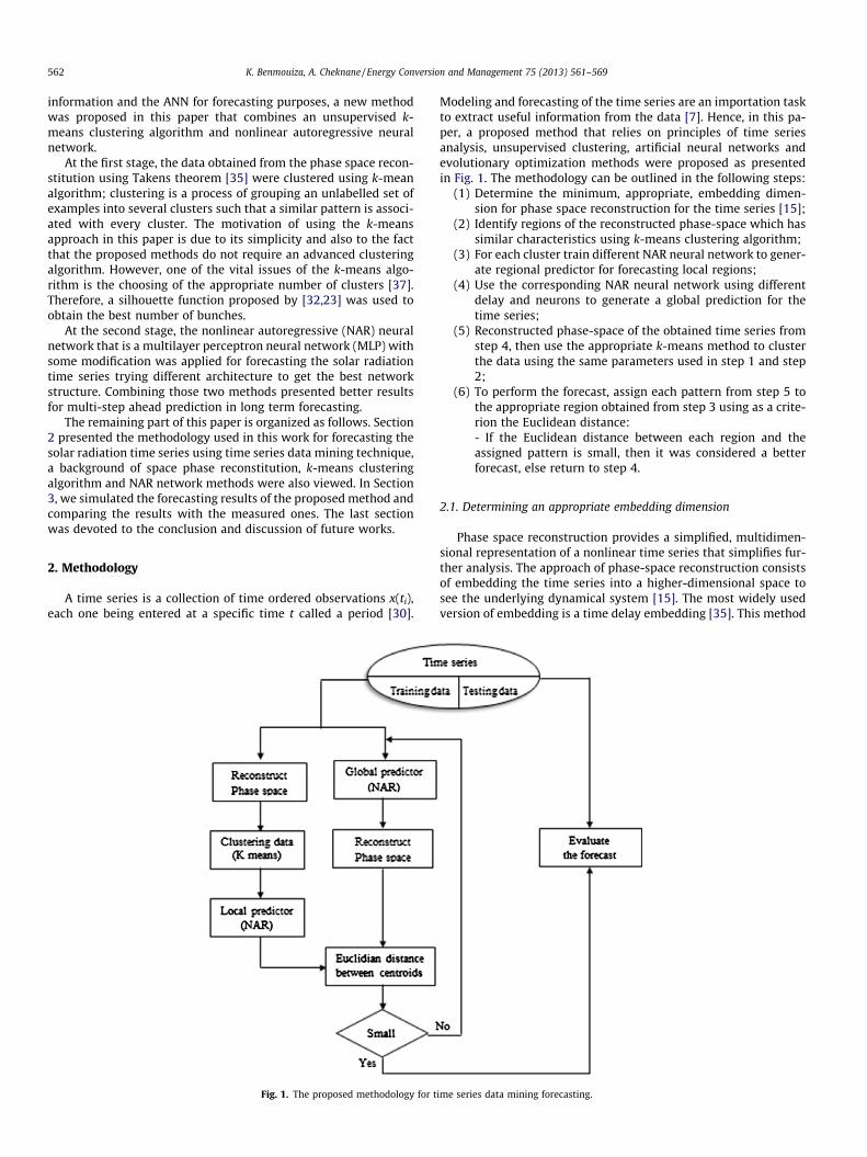
2.2. k-Means algorithm

k-Means is one of the quickest and simplest unsupervised learn-ing algorithms to perform clustering; the method consists of clas-sifying a given data into fixed k clusters [25,34]. The main idea is todefine k centroids for each cluster; those centroids should beplaced as much as possible far away from each other. In first step,each point of the data set is connected to the nearest cluster cen-troid by calculating the squared Euclidian distance between datapoint xðjÞi and the cluster centre c

j, as expressed by the following

equation

kxðjÞi � cjk2 ð4Þ

The second step consists of re-calculating the location of thenew k centroid. Repeating the first and second steps until the cen-troids no longer move produced a separation of the objects intogroups from which the objective function J expressed in Eq. (5) isminimized.

J ¼Xk

j¼1

Xn

i¼1

kxðjÞi � cjk2 ð5Þ

A summary of k-means algorithm is shown in Fig. 2,

2.2.1. Selection of the number of clustersThe k-means algorithm is based on the selection of the opti-

mum number of clusters [34,37]. The choosing of many clustersdoes not necessarily imply having a better quality of information.On the other hand, a small number of clusters produce unclear re-sults that could muddle the pattern recognition up.

The Silhouette function [32] expressed in Eq. (6) provides ameasure of the cluster separation that can be used for the interpre-tation and validation of clustered data. The motivation of using thistechnique that is simple to read, and provides a graphical represen-tation that allows the testing of various sets of clusters. It consistsof calculating the average dissimilarity a (i) of the ith data withinthe same cluster. This criterion can be interpreted as how well-matched the ith data to those clusters are assigned to it. The nextstep, is to determine the average dissimilarity of the ith data withthe data of another cluster, then the lowest average is denoted byb(i).

sðiÞ ¼ bðiÞ � aðiÞmaxfaðiÞ; bðiÞg ð6Þ

From this equation, it is clearly shown that if s(i) is close to 1then a(i)� b(i), which means that the values of a(i) are too small,which indicate that the ith data is well matched for its cluster. Fur-thermore, a large b(i) implies that i is badly matched to its neigh-boring cluster. Thus, a s(i) close to 1 means that the datum isappropriately clustered. If s(i) is close to minus one, then by thesame logic, we can see that i would be more appropriate if it wasclustered in its neighboring cluster. An s(i) near zeromeans thatthe datum is on the border of two natural clusters.

A successful clustering has a high mean silhouette value s(i).Lletí et al. [23] considered a 0.6 silhouette value for all clustersas a good result. However, in real-time series, it is almost impossi-ble to achieve this. Hence, a compromise among silhouette plotsand averages was used to determine the natural number of clusterswithin a data set.

2.3. Nonlinear autoregressive neural network (NAR)

Artificial neural network (ANN) is a class of neural network rep-resented by a mathematical model that is inspired by the biologicalnervous system; it is an intelligent system that has the ability torecognize time series patterns and nonlinear characteristics.

564 K. Benmouiza, A. Cheknane / Energy Conversion and Management 75 (2013) 561–569

Hence, it has been widely used for modeling dynamic nonlineartime series [13,22].

ANN combines artificial neurons to process information; it ismade up by simple neurons that are connected in a network byweighted links. Each input is multiplied by those weights thatcomputed by a mathematical function which defines the activationof the neuron. Another activation function computes the output ofthe artificial neuron that depends on a certain threshold.

Using mathematical notation, the output of a neuron can bewritten as the following equation,

y ¼ f bþX

i

wixi

!ð7Þ

here b is the bias for the neuron; the bias input to the neuronalgorithm is an offset value that helps the signal to exceed the acti-vation function’s threshold. f is the activation function, w

iare the

weights, xiare the inputs and y represents the output.

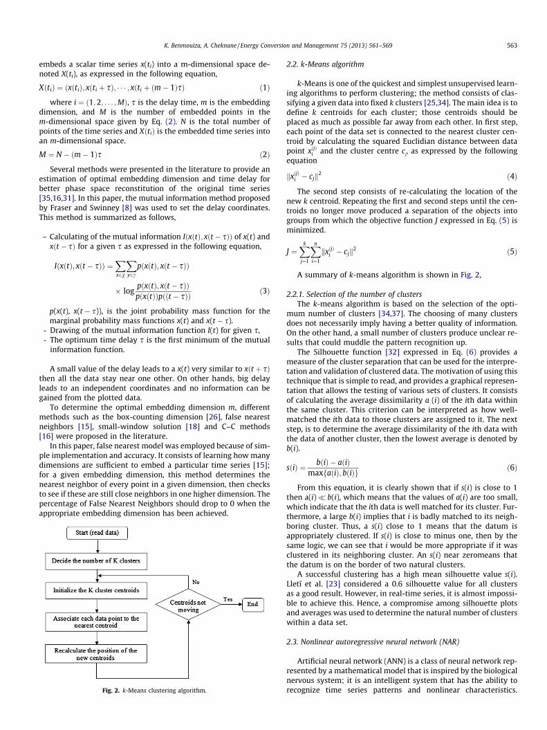
Various types of artificial neural networks were presented inliterature among them Multi-Layer Perceptron (MLP), where theneurons are grouped into an input layer, one or more hidden layersand an output layer. Recurrent Neural Networks (RNN) such aslayer recurrent networks [13], Time Delay Neural Networks(TDNN) [13,36] and NAR [6,27]. In RNN, the outputs of a dynamicsystem depend not only on the present inputs, but also on the his-tory of the states systems and the inputs. The NAR is a recurrentdynamic network based on a linear autoregressive model withfeedback connections, including several layers of the network. Itis commonly used in multi-step ahead time series forecasting; ituses past values of the actual time series to predict next valuesas determined by the following equation,

yðtÞ ¼ f yðt � 1Þ þ yðt � 2Þ þ � � � þ yðt � dÞð Þ ð8Þ

f is a nonlinear function, where the future values depend onlyon regressed d previous values of the output signal as shown inFig. 3. The combined history of the inputs and outputs of the sys-tem forms an intermediate inputs vector to be shown in the neuralnetwork model that could be any of the standard feed forward neu-ral networks like MLP networks.

In addition, the RNN are based on training algorithms that usedto adjust the weight values to get a desired output when certain in-puts are given. Hence, various ways were presented to let a neuralnetwork learn such as supervised training where the input–outputset is defined, and unsupervised learning that the output isundefined.

Back-propagation method is one of the most popular andwidely used learning techniques for training RNN. It consists ofminimizing the global quadratic error between the network output

Fig. 3. Structure of

and the desired target by adjusting the weight values. The adjust-ment can be done using several algorithms such as Levemberg–Marquardt [19,25], Bayesian Regularization [24] and scaledconjugate gradient [29] algorithms. The latter one was selectedto train larger networks. Once the network is trained using thepreselected inputs and outputs, all the synaptic weights are saved,and the network is ready to be tested on the new input informa-tion. Since the NAR network is very similar to a Multilayer Percep-tron (MPL), a modified MLP neural network was applied in thispaper for predicting purposes.

3. Simulation results

In our simulation, we are interested in multi-hour ahead fore-casting of the hourly global solar radiation time series using a com-bination of clustering techniques and nonlinear autoregressiveneural networks. Hence, two global horizontal solar radiation timeseries were selected in this paper for simulation purposes. In allcases, the evaluation of the accuracy of the prediction methodologyis accomplished by calculating the root mean square error (RMSE)expressed by Eq. (9) and the normalized root mean square error(NRMSE) given by Eq. (10),

RMSE ¼ < ðIi;predicted � Ii;measuredÞ2 >h i1

2 ð9Þ

NRMSE ¼< ðIi;predicted � Ii;measuredÞ2 >h i1

2

< Ii;measured >

0B@

1CA ð10Þ

RMSE and NRMSE provide information on the short-term per-formance of the correlations by allowing a term-by-term compar-ison of the actual difference between the predicted and measuredvalues. An NRMSE value between 0.2 and 0.5 was considered byLewis [20] to be as a good prediction model. Kostylev and Pavlovski[17] found that the best performing model on an hourly time scalehad an NRMSE of 0.17 for mostly clear days and 0.32 for mostlycloudy days. Furthermore, Wu and Chan [36] found that theNRMSE error will be big in the case of cloudy skies.

In addition, a comparison between the introduced naïve autore-gressive and moving average (ARMA) predictors was used to eval-uate the goodness of the proposed method. ARMA model has beenwidely used in papers for forecasting solar radiation time series[36]. It consists of modeling a time series of its past values, asexpressed in the following equation,

xt ¼Xp

i¼1

uixt�i þ et þXq

j

hjet�j ð11Þ

NAR network.

0 0.2 0.4 0.6 0.8 1

1

2

3

Silhouette Value

Clu

ster

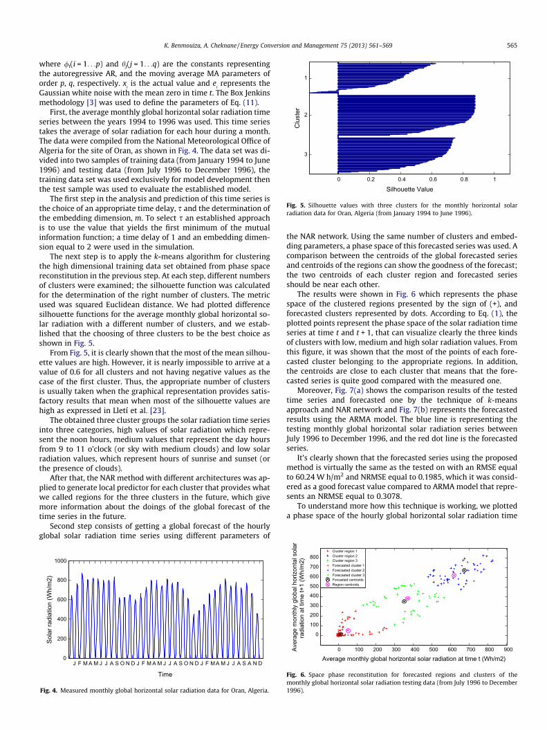
Fig. 5. Silhouette values with three clusters for the monthly horizontal solarradiation data for Oran, Algeria (from January 1994 to June 1996).

K. Benmouiza, A. Cheknane / Energy Conversion and Management 75 (2013) 561–569 565

where /i(i = 1. . .p) and hj(j = 1. . .q) are the constants representingthe autoregressive AR, and the moving average MA parameters oforder p, q, respectively. x

tis the actual value and e

trepresents the

Gaussian white noise with the mean zero in time t. The Box Jenkinsmethodology [3] was used to define the parameters of Eq. (11).

First, the average monthly global horizontal solar radiation timeseries between the years 1994 to 1996 was used. This time seriestakes the average of solar radiation for each hour during a month.The data were compiled from the National Meteorological Office ofAlgeria for the site of Oran, as shown in Fig. 4. The data set was di-vided into two samples of training data (from January 1994 to June1996) and testing data (from July 1996 to December 1996), thetraining data set was used exclusively for model development thenthe test sample was used to evaluate the established model.

The first step in the analysis and prediction of this time series isthe choice of an appropriate time delay, s and the determination ofthe embedding dimension, m. To select s an established approachis to use the value that yields the first minimum of the mutualinformation function; a time delay of 1 and an embedding dimen-sion equal to 2 were used in the simulation.

The next step is to apply the k-means algorithm for clusteringthe high dimensional training data set obtained from phase spacereconstitution in the previous step. At each step, different numbersof clusters were examined; the silhouette function was calculatedfor the determination of the right number of clusters. The metricused was squared Euclidean distance. We had plotted differencesilhouette functions for the average monthly global horizontal so-lar radiation with a different number of clusters, and we estab-lished that the choosing of three clusters to be the best choice asshown in Fig. 5.

From Fig. 5, it is clearly shown that the most of the mean silhou-ette values are high. However, it is nearly impossible to arrive at avalue of 0.6 for all clusters and not having negative values as thecase of the first cluster. Thus, the appropriate number of clustersis usually taken when the graphical representation provides satis-factory results that mean when most of the silhouette values arehigh as expressed in Lletí et al. [23].

The obtained three cluster groups the solar radiation time seriesinto three categories, high values of solar radiation which repre-sent the noon hours, medium values that represent the day hoursfrom 9 to 11 o’clock (or sky with medium clouds) and low solarradiation values, which represent hours of sunrise and sunset (orthe presence of clouds).

After that, the NAR method with different architectures was ap-plied to generate local predictor for each cluster that provides whatwe called regions for the three clusters in the future, which givemore information about the doings of the global forecast of thetime series in the future.

Second step consists of getting a global forecast of the hourlyglobal solar radiation time series using different parameters of

J F M A M J J A S O N D J F M A M J J A S O N D J F MA M J J A S A N D0

200

400

600

800

1000

Time

Sola

r rad

iatio

n (W

h/m

2)

Fig. 4. Measured monthly global horizontal solar radiation data for Oran, Algeria.

the NAR network. Using the same number of clusters and embed-ding parameters, a phase space of this forecasted series was used. Acomparison between the centroids of the global forecasted seriesand centroids of the regions can show the goodness of the forecast;the two centroids of each cluster region and forecasted seriesshould be near each other.

The results were shown in Fig. 6 which represents the phasespace of the clustered regions presented by the sign of (+), andforecasted clusters represented by dots. According to Eq. (1), theplotted points represent the phase space of the solar radiation timeseries at time t and t + 1, that can visualize clearly the three kindsof clusters with low, medium and high solar radiation values. Fromthis figure, it was shown that the most of the points of each fore-casted cluster belonging to the appropriate regions. In addition,the centroids are close to each cluster that means that the fore-casted series is quite good compared with the measured one.

Moreover, Fig. 7(a) shows the comparison results of the testedtime series and forecasted one by the technique of k-meansapproach and NAR network and Fig. 7(b) represents the forecastedresults using the ARMA model. The blue line is representing thetesting monthly global horizontal solar radiation series betweenJuly 1996 to December 1996, and the red dot line is the forecastedseries.

It’s clearly shown that the forecasted series using the proposedmethod is virtually the same as the tested on with an RMSE equalto 60.24 W h/m2 and NRMSE equal to 0.1985, which it was consid-ered as a good forecast value compared to ARMA model that repre-sents an NRMSE equal to 0.3078.

To understand more how this technique is working, we plotteda phase space of the hourly global horizontal solar radiation time

0 100 200 300 400 500 600 700 800 900

0

100

200

300

400

500

600

700

800

Average monthly global horizontal solar radiation at time t (Wh/m2)

Aver

age

mon

thly

glo

bal h

oriz

onta

l sol

ar

Cluster region 1Cluster region 2Cluster region 3Forecasted cluster 1Forecasted cluster 2Forecasted cluster 3Forcasted centroidsRegion centroids

radi

atio

n at

tim

e t+

1 (W

h/m

2)

Fig. 6. Space phase reconstitution for forecasted regions and clusters of themonthly global horizontal solar radiation testing data (from July 1996 to December1996).

1st Jun. Jul. Aug. Sep. Oct. Nov. 31st Dec.

0

200

400

600800

1000

0

200400

Time (months)

Aver

age

mon

thly

hor

izon

tal g

loba

l

forecasted solar radiationmeasured solar radiation

sola

r rad

iatio

n (W

h/m

2)

Fig. 7a. Comparison between measured monthly global horizontal solar radiationdata (from July 1996 to December 1996), and forecasted by the proposed model.

1st Jun. Jul. Aug. Sep. Oct. Nov. Dec.

0

200

400

600

800

Time (months)

Aver

age

mon

thly

glo

bal h

oriz

onta

l Measured solar radiationForecasted sola radiation

sola

r rad

iatio

n (W

/m2)

Fig. 7b. Comparison between measured monthly global horizontal solar radiationdata (from July 1996 to December 1996), and forecasted by ARMA model.

1st Jun. Jul. Aug. Sep. Oct. Nov. 31st Dec.

0

100

200

300

400

500

600

700

800

Time (months)

Aver

age

mon

thly

hor

izon

tal g

loba

l sol

ar

Measured solar radiationForecasted solar radiation

radi

atio

n (W

h/m

2)

Fig. 9. Comparison between measured monthly global horizontal solar radiationdata (from July 1996 to December 1996), and forecasted by proposed model usingwrong parameters.

1 st Jan. 50 100 150 200 250 300 350 400 31 Jan.

200

400

600

800

1000

Time (hours)

Hou

rly

glob

al h

oriz

onta

l sol

ar

radi

atio

n (W

h/m

2)

Fig. 10a. Measured hourly global horizontal solar radiation time series for January

566 K. Benmouiza, A. Cheknane / Energy Conversion and Management 75 (2013) 561–569

series at time t and t + 1, but with wrong NAR network parameters,as shown in Fig. 8. It can observe from this figure that the points ofthe clusters are mixed with each other. In addition, the centroidsare too far from each other, especially for the cluster 2 and 3, lead-ing to the fact that the obtained forecast is not good comparing bythe test one as shown in Fig. 9, which represented the forecastedaverage monthly global solar radiation series in red and the testedseries in blue, representing an NRMSE error equals to 0.5532 that isnot good forecast value.

In the same way, we used this methodology for morecomplicated solar radiation time series that provides forecasts atone-hour time step, which used widely in a lot of solar radiationapplication. Hence, an hourly global horizontal solar radiation timeseries for the year of 1996 was then applied.

The data were collected from the National Meteorological Officeof Algeria for the site of Oran. We used only the data from sunrise

-100 0 100 200 300 400 500 600 700 800-100

0

100

200

300

400

500

600

700

800

Average monthly global horizontal solar radiation at time t (Wh/m2)

Aver

age

mon

thly

glo

bal h

oriz

onta

l sol

ar

Cluster region 1Cluster region 2Cluster region 3Forecasted cluster 1Forecasted cluster 2Forecasted cluster 3Forecasts centroidsRegion centroids

radi

atio

n at

tim

e t+

1 (W

h/m

2)

Fig. 8. Space phase reconstitution for forecasted regions and clusters of themonthly global horizontal solar radiation testing data (from July 1996 to December1996) using wrong parameters.

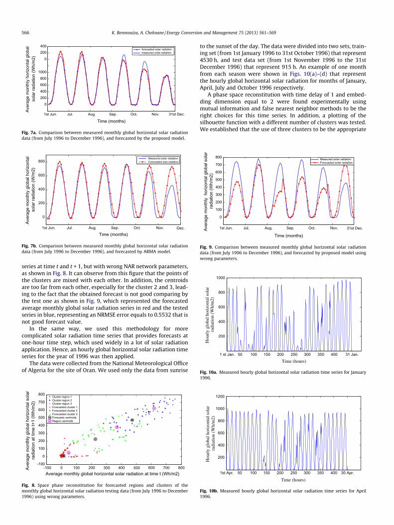
to the sunset of the day. The data were divided into two sets, train-ing set (from 1st January 1996 to 31st October 1996) that represent4530 h, and test data set (from 1st November 1996 to the 31stDecember 1996) that represent 915 h. An example of one monthfrom each season were shown in Figs. 10(a)–(d) that representthe hourly global horizontal solar radiation for months of January,April, July and October 1996 respectively.

A phase space reconstitution with time delay of 1 and embed-ding dimension equal to 2 were found experimentally usingmutual information and false nearest neighbor methods to be theright choices for this time series. In addition, a plotting of thesilhouette function with a different number of clusters was tested.We established that the use of three clusters to be the appropriate

1996.

1st Apr. 50 100 150 200 250 300 350 400 30 Apr.

200

400

600

800

1000

1200

Time (hours)

Hou

rly

glob

al h

oriz

onta

l sol

ar

radi

atio

n (W

h/m

2)

Fig. 10b. Measured hourly global horizontal solar radiation time series for April1996.

K. Benmouiza, A. Cheknane / Energy Conversion and Management 75 (2013) 561–569 567

choice as represented in Fig. 11, which represented the silhouettefunction of the hourly global horizontal solar radiation time series.It is clearly shown that the three clusters are well separated withthe most of the points are above 0.6, except some negative onesin the second cluster that we can consider to be normal for suchnonlinear time series.

For calculating the hourly global solar radiation time series, thek-means algorithm was then applied to clustering the trainingdata. A local predictor was applied for obtaining future regions;those regions represent future windows for the forecasted data.Then, the NAR method with different time delay and neuronswas applied to create global predictor of the data. The use of 25 de-lays with 13 neurons was found as the right choice for forecastingpurpose. The results of phase space reconstitution of the forecastedregions and clusters for the hourly global horizontal solar radiation

1st Jul. 50 100 150 200 250 300 350 400 31 Jul.

200

400

600

800

Time (hours)

Hou

rly g

loba

l hor

izon

tal s

olar

ra

diat

ion

(Wh/

m2)

Fig. 10c. Measured hourly global horizontal solar radiation time series for July1996.

1st Oct. 50 100 150 200 250 300 350 400 31 Oct.

200

400

600

800

Time (hours)

hour

ly g

loba

l hor

izon

tal s

olar

ra

diat

ion

(Wh/

m2)

Fig. 10d. Measured hourly global horizontal solar radiation time series for October1996.

-0.2 0 0.2 0.4 0.6 0.8 1

1

2

3

Silhouette Value

Clu

ster

Fig. 11. Silhouette values with 3 clusters for the hourly global horizontal solarradiation data for Oran, Algeria (from 1st January 1996 to 31st October 1996).

at time t and t + 1 considering a time delay of 1 and embeddingdimension of 2 was presented in Fig. 12.

From Fig. 12, the most of the points of each forecast cluster arein the right regions, the centroids are near each other, which meanthat the obtained forecast is acceptable. The comparison betweenthe forecasted hourly global horizontal solar radiation data andthe tested data is shown in Fig. 13(a).

In addition, Figs. 13(b) and (c) represent the comparison resultsfor the months of November 1996 and December 1996 respec-tively. The blue line represents measured data, and the red one isthe forecasted data.

Moreover, the performance of the forecasted hourly global hor-izontal time series has been evaluated by calculating the RMSE er-rors between the actual data and forecasted one for the period of1st November 1996 to 31st December 1996. The quadratic errorbetween measured and simulated hourly global solar radiationusing the proposed method was presented in Fig. 14. In addition,Fig. 15 represents the measured time series versus the forecastedtime series.

From Fig. 14, the total RMSE was equal to 64.34 W h/m2 and theNRMSE was 0.2003, which can be viewed as good forecasted valuescompared with an NRMSE equal to 0.3184 by using the baselineARMA model.

In addition, from Fig. 15, the R squared value calculated by Eq.(12) is equal to 0.9330. The most of the points of the forecastedand measured series are near each to other. However, it presentssome lags due to the total covered days that present a lot of clouds.Finally, from the simulation results, this methodology was con-ceived to be such a good method to perform the forecast results.

-200 0 200 400 600 800 1000-200

0

200

400

600

800

1000

Hourly global horizontal solar radiation at time t (Wh/m2)

Hou

rly g

loba

l hor

izon

tal s

olar

radi

atio

n

Cluster region 1Cluster region 2Cluster region 3Forecasted cluster 1Forecasted cluster 2Forecasted cluster 3Forecasted centroidsRegion centroids

at ti

me

t+1

(Wh/

m2)

Fig. 12. Space phase reconstitution for the forecasted regions and clusters of thehourly global horizontal solar radiation testing data (from 1st November 1996 tothe 31st December 1996).

0 100 200 300 400 500 600 700 800 900 10000

100

200

300

400

500

600

700

800

900

1000

Time (hours )

Hou

rly g

loba

l hor

izon

tal s

olar

Measured solar radiationForecasted solar radiation

radi

atio

n (W

h/m

2)

Fig. 13a. Comparison between measured hourly global horizontal solar radiation(from 1st November 1996 to the 31st December 1996) and forecasted by theproposed model.

1st Nov. 50 100 150 200 250 300 350 400 30 Nov.0

200

400

600

800

1000

Time (hours)

Hou

rly

glob

al h

oriz

onta

l sol

ar Measured dataForecasted data

radi

atio

n (W

h/m

2)

Fig. 13b. Comparison between measured hourly global horizontal solar radiation(from 1st November 1996 to the 31st November 1996) and forecasted by theproposed model.

1st Dec. 500 550 600 650 700 750 800 850 31 Dec.0

200

400

600

800

1000

Time (hours)

Hou

rly

glob

al h

oriz

onta

l sol

ar) Measured data

Forecasted data

radi

atio

n (W

h/m

2

Fig. 13c. Comparison between measured hourly global horizontal solar radiation(from 1st December 1996 to the 31st December 1996) and forecasted by theproposed model.

0 100 200 300 400 500 600 700 800 900 10000

2

4

6

8

10

12

14

Time (hours)

Aver

age

of q

uada

ratic

erro

r (W

h/m

2) Average of quadaratic error

Fig. 14. the quadratic error between measured global horizontal solar radiation(from 1st November to 31st December 1996) and the forecasted using the proposedmodel.

0 100 200 300 400 500 600 700 800 900 1000-200

0

200

400

600

800

1000

Measured hourly global solar radiation (Wh/m2)

Fore

cast

ed h

ourly

glo

bal s

olar

Measured solar radiationForecasted solar radiation

R squared value : 0.9330

radi

atio

n (W

h/m

2)

Fig. 15. The measured hourly global horizontal from (1st November 1996 to 31stDecember 1996) versus forecasted time series using the proposed model.

568 K. Benmouiza, A. Cheknane / Energy Conversion and Management 75 (2013) 561–569

R2 ¼

Pni¼1ðIi;measured � Ii;measured

�Þ

2� �Pn

i¼1ðIi;predicted � Ii;measured

�Þ

2� �

0BB@

1CCA ð12Þ

4. Conclusion

In this paper, we presented a time series forecasting methodol-ogy based on the clustering methods and artificial neural networks.The methodology consists of three essential stages. First, phasespace reconstitution of the hourly global solar radiation time serieswas reached by finding the appropriate time delay using mutualinformation method, and the minimum embedding dimension isdefined using false nearest neighbor method. Secondly, theunsupervised k-means clustering algorithm was then applied forgrouping the input data into k clusters, which have similar charac-teristics. For choosing of the right number of clusters, the silhou-ette plot which represents a graphical representation of theseparation of the heads of each cluster from another one was thenused. Subsequently, a different NAR neural network was preparedon each cluster to act as a local predictor for the correspondingsubspace of the input space. In addition, another NAR networkwas used to act as a global predictor for the solar radiation timeseries. The methodology was applied to generate multi-step aheadforecasts for the hourly global horizontal solar radiation timeseries. The obtained experimental results showed that the cluster-ing of the input space is an important task to interpret the behaviorof the series. Moreover, identifying forecasted regions using NARnetwork provides additional information about future patternsthat can simplify the analysis of the global forecast of the series.In addition, the proposed method does not need a complicateclustering algorithm. Hence, as a conclusion of this work, the timeseries data mining method was considered such a good way offorecasting such similar problems. Nevertheless, this methodpresents some limitations for the total covered sky where the pres-ence of clouds is heavy, also the calculation time, especially in thepreparation phase of the NAR network. Hence, future works, willbe focused on testing different clustering algorithms and differentartificial neural networks to improve the forecasting performancethat improves the reliability in the case of covered sky.

Acknowledgement

The authors would like to thank the University of Laghouat forthe financial aspect of the present work.

References

[1] Maia André Luis S, de Carvalho ATFrancisco, Teresa BL. Forecasting models forinterval-valued time series. Neurocomputing 2008;71:3344–52.

[2] Azadeh A, Maghsoudi A, Sohrabkhani S. An integrated artificial neuralnetworks approach for predicting global radiation. Energy Convers Manage2009;50:1497–505.

[3] Box GEP, Jenkins G. Time series analysis. Holden-Day (San Francisco,CA): Forecasting and Control; 1970.

[4] Celik AN, Muneer T. Neural network based method for conversion of solarradiation data. Energy Convers Manage 2013;67:117–24.

[5] Chen SX, Gooi HB, Wang MQ. Solar radiation forecast based on fuzzy logic andneural networks. Renew Energy 2013;60:195–201.

[6] Chow TWS, Leung CT. Non-linear autoregressive integrated neural networkmodel for short term load forecasting. IEE Proc Gen Trans Distribut1996;143:500–6.

[7] Faraway JJ, Chatfield C. Time series forecasting with neural networks: a casestudy. Statistics Group Research Report 9506, University of Bath; 1995.

[8] Fraser M, Swinney L. Independent coordinates for strange attractors frommutual information. Phys Rev A 1986;33:1134–40.

[9] Fu T. A review on time series data mining. Eng Appl Artif Intell2011;24:164–81.

[10] Gelman R. 2011 Renewable energy data book (Revised Book). Efficiency RenewEnergy (EERE) 2013.

K. Benmouiza, A. Cheknane / Energy Conversion and Management 75 (2013) 561–569 569

[11] Huang Y. Advances in artificial neural networks-methodological developmentand application. Algorithms 2009;2:973–1007.

[12] Huang J, Korolkiewicz M, Agrawal M, Boland J. Forecasting solar radiation onan hourly time scale using a Coupled AutoRegressive and Dynamical System(CARDS) model. Sol Energy 2013;87:136–49.

[13] Haykin S. Neural networks: a comprehensive foundation. 2nd ed. PrenticeHall; 1998.

[14] Kaplanis S. New methodologies to estimate the hourly global solar radiation;comparisons with existing models. Renew Energy 2006;31:781–90.

[15] Kennel MB, Brown R, Abarbanel HD. Determining embedding dimension forphase space reconstruction using a geometrical construction. Phys Rev A1992;45(6):3403–11.

[16] Kim HS, Eykholt R, Salas JD. Nonlinear dynamics, delay times, and embeddingwindows. Physica D 1999;127:48–60.

[17] Kostylev V, Pavlovski A. Solar power forecasting performance – towardsindustry standards, In: Proceedings of the 1st international workshop on theintegration of solar power into power systems, Aarhus, Denmark; 2011

[18] Kugiumtzis D. State space reconstruction parameters in the analysis of chaotictime series—the role of the time window length. Physica D 1996;95:13–28.

[19] Levenberg K. A method for the solution of certain problems in least squares. QAppl Math 1944;5:164–8.

[20] Lewis CD. International and business forecasting methods. London: Butter-Worths; 1982.

[21] Liao S, Chu P, Hsiao P. Data mining techniques and applications – a decadereview from 2000 to 2011. Expert Syst Appl 2012;39:11303–11.

[22] Ljung L. System identification: theory for the user. 2nd ed. Prentice Hall PTR;1998.

[23] Lletí R, Ortiz MC, Sarabia LA, Sánchez MS. Selecting variables for k-meanscluster analysis by using a genetic algorithm that optimises the silhouettes.Anal Chim Acta 2004;515:87–100.

[24] MacKay DJC. Bayesian interpolation. Neural Comput 1992;4(3):415–47.[25] MacQueen JB. Some methods for classification and analysis of multivariate

observations. In: Proceedings of 5th Berkeley symposium on mathematicalstatistics and probability 1. University of California Press; 1967. p. 281–297.

[26] Mandelbrot BB. How long is the coastline of Britain? Statistical self-similarityand fractional dimension. Science 1967;155:636.

[27] Markham IS, Rakes TR. The effect of sample size and variability of data on thecomparative performance of artificial neural networks and regression. ComputOper Res 1998;25:251–63.

[28] Mellit A, Kalogirou SA, Hontoria L, Shaari S. Artificial intelligence techniquesfor sizing photovoltaic systems: a review. Renew Sustain Energy Rev2009;13(2):406–19.

[29] Moller MF. A scaled conjugate gradient algorithm for fast supervised learning.Neural Networks 1993;4:525–33.

[30] Pandit SM, Wu SM. Time series and system analysis, with applications; 1983.[31] Ragulskis M, Lukoseviciute K. Non-uniform attractor embedding for time

series forecasting by fuzzy inference systems. Neurocomputing2009;72:2618–26.

[32] Rousseeuw J. Silhouettes: a graphical Aid to the interpretation and validationof cluster analysis. Comput Appl Math 1987;20:53–65.

[33] Sandberg I, Xu L. Uniform approximation of multidimensional myopic maps.IEEE Trans Circ Syst I: Fund Theory Appl 1997;44(6):477–85.

[34] Spath H. Cluster dissection and analysis: theory, Fortran programs, examplestranslated by J. Goldschmidt. New York: Halsted Press; 1985. 226 pp.

[35] Takens F. Detecting strange attractors in turbulence, Dynamical Systems andTurbulence In: Rand DA, Young LS. editors, Lecture notes in mathematics. vol.898; 1981. p. 366-381.

[36] Wu J, Chan KC. Prediction of hourly solar radiation using a novel hybrid modelof ARMA and TDNN. Sol Energy 2011;85:808–17.

[37] Xu R, Donald C. Survey of clustering algorithm. IEEE Trans Neural Networks2005;16(3):46–51.

[38] Zeng Z, Yang H, Zhao R, Meng J. Nonlinear characteristics of observed solarradiation data. Sol Energy 2013;87:204–18.

[39] Zhang G. Time series forecasting using a hybrid ARIMA and neural networkmodel. Neurocomputing 2003;50:159–75.

[40] Boland JW. Time series and statistical modelling of solar radiation, RecentAdvances in Solar Radiation Modelling, Viorel Badescu (Ed.), Springer-Verlag2008; 283-312.