Forecasting Ex-Vessel Prices for Hard Blue Crabs in the Chesapeake Bay Region: Individual and Composite Methods Michael A. Hudson and Oral Capps, Jr.

Given the relative importance of the Chesapeake Bay hard blue crab fishery to the U .S. blue crab fishery , this paper analyzes ex-vessel prices for hard blue crabs landed in this region. The purpose is to evaluate a lternative methods of forecasting ex-vessel prices for hard blue crabs in the Bay; both individual methods (trend extrapolation, econometric, and time-series) and composite methods. Examining the mean squared errors for the individual methods, the time-series model performs the best, with the econometric model slightly better than the trend extrapolation model. None of the composite methods outperforms the time-series model , although in some cases the differences are slight. Nevertheless, the time-series trend extrapolation composite outperforms all other models in identifying turning points. Generally speaking, it would appear that ex-vessel prices for hard blue crabs possess strong time dependencies , and consequently, better forecasts occur with time-series models than with econometric models.

Introduction

Hard blue crabs are prevalent primarily on the East and Gulf coasts of the United States. The economic importance of hard blue crabs to these regions has long been recognized. In the last twenty years, the average annual produc­tion has been approximately 140 million pounds , valued at roughly 15 million dollars.

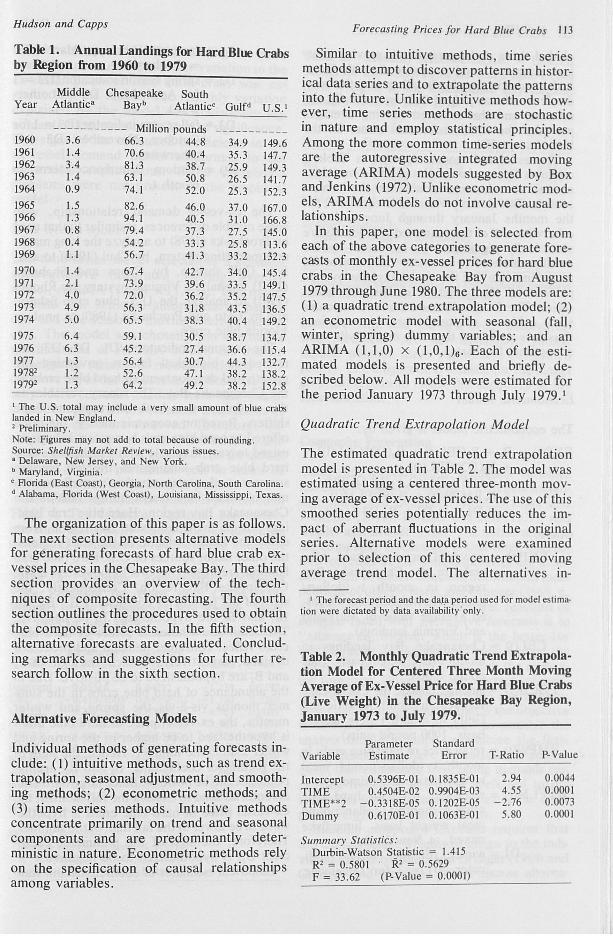
Hard blue crabs are more abundant in the Chesapeake Bay than elsewhere. Annual land­ings for hard blue crabs from 1960 to 1979 in the Chesapeake Bay have ranged from 45.2 to 94.1 million pounds, 0.4 to 6.4 million pounds in the Middle Atlantic, 27.4 to 52.0 million pounds in the South Atlantic, and 25.3 to 44.3 million pounds in the Gulf (Table 1). On aver­age, the Chesapeake Bay region has accounted for 46 percent of the hard blue crab landings in the United States over this period . The aver­age annual share of hard blue crab landings for the Middle Atlantic, South Atlantic, and Gulf regions has been 2, 28, and 24 percent, respec­tively (Shellfish Market Review).

Given the relative importance of the Chesapeake Bay hard blue crab fishery to the

The authors are , respectively, Research Associate in the De­partment of Agricultural Economics and Assistant Professor in the Department of Agricultural Economics and in the Department of Statistics, Virginia Tech , Blacksburg, Virginia .

U.S. blue crab fishery, this paper analyzes ex-vessel prices for hard blue crabs landed in this region. Ex-vessel prices are defined by the U.S. Department of Commerce as "prices re­ceived by harvesters for fish and shellfish landed at the dock.'' Except for the work of Cato and Prochaska (1980) and Rhodes (1981), little attention has been focused on ex-vessel prices for hard blue crabs . This study concentrates on hard blue crabs because the aggregate ex-vessel value of hard blue crab landings has constituted more than 80 percent of the aggregate ex-vessel value of total blue crab landings in the United States since 1952 (Rhodes 1981).

Harvesters in the acquacultural sector as well as producers in the agricultural sector make decisions in risky environments . Ra­tional decision-making consequently requires information about the likelihood of many al­ternative outcomes. This information is gener­ally available from both private and public sources in the way of price forecasts. In this light, the specific purpose of tbis paper is to evaluate alternative methods, both individual and composite, of forecasting ex-vessel prices for hard blue crabs in the Chesapeake Bay region . This research is likely to pay dividends in the way of assessment of price forecast information, to harvesters of hard blue crabs in the Chesapeake Bay region.

Hudson and Capps

Table 1. Annual Landings for Hard Blue Crabs by Region from 1960 to 1979

Middle Chesapeake South Year Atlantic• Bay• Atlanticc GuJfd U.S.'

----------- Million pounds -----------1960 3.6 66.3 44.8 34.9 149.6 1961 1.4 70.6 40.4 35.3 147.7 1962 3.4 81.3 38.7 25.9 149.3 1963 1.4 63.1 50.8 26.5 141.7 1964 0.9 74.1 52.0 25.3 152.3 1965 1.5 82.6 46.0 37.0 167.0 1966 1.3 94.1 40.5 31.0 166.8 1967 0.8 79.4 37.3 27.5 145.0 1968 0.4 54.2 33.3 25.8 113.6 1969 1.1 56.7 41.3 33.2 132.3 1970 1.4 67.4 42.7 34.0 145.4 1971 2.1 73.9 39.6 33.5 149.1 1972 4.0 72.0 36.2 35.2 147.5 1973 4.9 56.3 31.8 43.5 136.5 1974 5.0 65 .5 38.3 40.4 149.2 1975 6.4 59.1 30.5 38.7 134.7 1976 6.3 45.2 27.4 36.6 115.4 1977 1.3 56.4 30.7 44.3 132.7 19782 1. 2 52.6 47.1 38.2 138.2 19792 1.3 64.2 49.2 38.2 152.8

1 The U.S. total may include a very small amount of blue crabs landed in New England. 2 Preliminary . Note: Figures may not add to total because of rounding. Source: Shellfish Market Review, various issues . • Delaware, New Jersey, and New York. • Maryland, Virginia. • Aorida (East Coast), Georgia, North Carolina, South Carolina. d Alabama, Aorida (West Coast), Louisiana, Mississippi , Texas.

The organization of this paper is as follows . The next section presents alternative models for generating forecasts of hard blue crab ex­vessel prices in the Chesapeake Bay. The third section provides an overview of the tech­niques of composite forecasting. The fourth section outlines the procedures used to obtain the composite forecasts. In the fifth section, alternative forecasts are evaluated. Conclud­ing remarks and suggestions for further re­search follow in the sixth section.

Alternative Forecasting Models

Individual methods of generating forecasts in­clude: (1) intuitive methods , such as trend ex­trapolation, seasonal adjustment, and smooth­ing methods; (2) econometric methods; and (3) time series methods. Intuitive methods concentrate primarily on trend and seasonal components and are predominantly deter­ministic in nature. Econometric methods rely on the specification of causal relationships among variables.

Forecasting Prices for Hard Blue Crabs 113

Similar to intuitive methods, time series methods attempt to discover patterns in histor­ical data series and to extrapolate the patterns into the future. Unlike intuitive methods how­ever, time series methods are stochastic in nature and employ statistical principles. Among the more common time-series models are the autoregressive integrated moving average (ARIMA) models suggested by Box and Jenkins (1972). Unlike econometric mod­els, ARIMA models do not involve causal re­lationships.

In this paper, one model is selected from each of the above categories to generate fore­casts of monthly ex-vessel prices for hard blue crabs in the Chesapeake Bay from August 1979 through June 1980. The three models are: (1) a quadratic trend extrapolation model; (2) an econometric model with seasonal (fall, winter, spring) dummy variables; and an ARIMA (1,1,0) x (1,0,1)6 • Each of the esti­mated models is presented and briefly de­scribed below. All models were estimated for the period January 1973 through July 1979. 1

Quadratic Trend Extrapolation Model

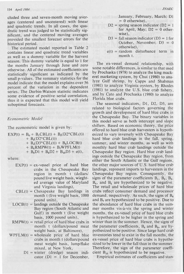
The estimated quadratic trend extrapolation model is presented in Table 2. The model was estimated using a centered three-month mov­ing average of ex-vessel prices. The use of this smoothed series potentially reduces the im­pact of aberrant fluctuations in the original series. Alternative models were examined prior to selection of this centered moving average trend model. The alternatives in-

1 The forecast period and the da.lfl period used for model estima­tion were dictated by data availability" only .

Table 2. Monthly Quadratic Trend Extrapola­tion Model for Centered Three Month Moving Average ofEx-Vessel Price for Hard Blue Crabs (Live Weight) in the Chesapeake Bay Region, January 1973 to July 1979.

Variable

Intercept TIME TIME**2 Dummy

Parameter Standard Estimate Error

0.5396E-01 0.1835&01 0.4504E-02 0.9904E-03

-0.33 18E-05 0.1202&05 0.6170&01 0.1063&01

Summary Statistics: Durbin-Watson Statistic = 1. 415 R2 = 0.5801 · R' = 0.5629 F = 33.62 (P-Value = 0.0001)

T-Ratio

2.94 4.55

-2.76 5.80

P-Value

0.0044 0.0001 0.0073 0.0001

114 April 1984

eluded three and seven-month moving aver­ages (centered and uncentered) with linear and quadratic trends. In all cases, the qua­dratic trend was judged to be statistically sig­nificant , and the centered moving averages provided the smallest forecast errors for the historical period.

The estimated model reported in Table 2 contains linear and quadratic trend variables as well as a dummy variable for the harvest season . This dummy variable is equal to 1 for the months January through June and zero otherwise. All of the estimated coefficients are statistically significant as indicated by the small p-values. The summary statistics for the model indicate that the model explains over 56 percent of the variation in the dependent series. The Durbin-Watson statistic indicates some evidence of positive serial correlation, thus it is expected that this model will yield suboptimal forecasts .

Econometric Model

The econometric model is given by:

EXP(t) = B0 + B1CBL(t) + B2(D2*CBL(t)) + B3(D2*CBL(t))

where:

+ BiD3*CBL(t)) + B5LOCB(t) + B6RMPW(t) + B7WPFLM(t) + B8D1 + B9D2 + B10D3 + e(t),

EXP(t) = ex-vessel price of hard blue crabs in the Chesapeake Bay region in month t (dollars/ pound Hve weight basis , wieght­ed average value of Maryland and Virginia landings) ,

CBL(t) = Chesapeake Bay landings in month t (live weight basis, 1000 pound units),

LOCB(t) = landings outside the Chesapeake Bay region (South Atlantic and Gulf) in month t (live weight basis , 1000 pound units),

RMPW(t) = retail price of hard blue crabs in month t (dollars/pound meat weight basis , at Baltimore),

WPFLM(t) = wholesale price of hard blue crabs in month t (dollars/pound meat weight basis , lump/flake mixed , at New York ,

Dl =winter (dredge) season indi­cator (DI = I for December,

JNAEC

January, February, March; D 1 = 0 otherwise),

D2 = spring season indicator (D2 = 1 for April, May; D2 = 0 other­wise),

D3 = fall season indicator (D3 = I for October, November; D3 = 0 otherwise) ,

e(t) = random disturbance term in month t.

The ex-vessel demand relationship , with some notable differences , is similar to that used by Prochaska (1978) to analyze the king mack­erel marketing system, by Chui (1980) to ana­lyze Gulf shrimp , by Capps and Shabman (1981) to analyze Virginia oysters, by Rhodes (1981) to analyze the U.S. blue crab fishery , and by Cato and Prochaska (1980) to analyze Florida blue crabs.

The seasonal indicators , DI , D2, D3, are related to biological factors governing the growth and development of hard blue crabs in the Chesapeake Bay. The binary variables in this model serve as both intercept and slope shifters. Based on economic theory , the price offered to hard blue crab harvesters is hypoth­esized to vary inversely with Chesapeake Bay hard blue crab landings in the fall, spring , summer, and winter months , as well as with monthly hard blue crab landings outside the Chesapeake Bay region . Hard blue crab land­ings outside the Chesapeake Bay region, from either the South Atlantic or the Gulf regions , the other major sources of U.S. hard blue crab landings , represent imports to harvesters in the Chesapeake Bay region. Consequently , the signs of the parameter coefficients B1 , B2 , B3 ,

B4 , and B5 are hypothesized to be negative. The retail and wholesale prices of hard blue crabs reflect consumer demand and processor demand , respectively. As such , the signs of B6

and B7 are hypothesized to be positive. Due to the abundance of hard blue crabs in the sum­mer months vis-a-vis the spring and winter months , the ex-vessel price of hard blue crabs is hypothesized to be higher in the spring and winter than in the summer. Hence , the signs of the parameter coefficients, B8 and B9 , are hy­pothesized to be positive. Since large hard crab inventories tend to exist in the fall months, the ex-vessel price of hard blue crabs is hypothe­sized to be lower in the fall than in the summer. Therefore, the sign of the parameter coeffi­cient B10 is hypothesized to be negative.

Empirical estimates of coefficients and stan-

Hudson and Capps

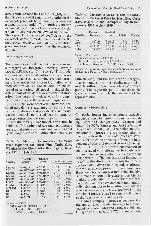
dard errors appear in Table 3. Slightly more than 80 percent of the monthly variation in the ex-vessel price of hard blue crabs was ex­plained by the model. The monthly variation explained by the model was statistically sig­nificant at any reasonable level of significance. The signs of the estimated coefficients in the ex-vessel demand model conformed to the theoretical expectations. Serial correlation problems were not present in the empirical model .

Time Series Model

The time series model selected is a seasonal autoregressive integrated moving average model, ARIMA (1,1,0) x (1,0,1)6 • This model contains one seasonal autoregressive param­eter and one seasonal moving average param­eter. The model was chosen from alternative specifications of ARIMA models for the ex­vessel price series. All models included first­differencing of the data series to obtain station­arity. Non-seasonal models were first exam­ined, but spikes at the seasonal frequencies of 6, 12, 18, etc. were observed. Therefore, sea­sonal models were examined for both six and twelve month seasonal periods. The six month seasonal models performed best in terms of forecast errors for the sample period .

The estimated ARIMA model is presented in Table 4. The estimated seasonal parameters are each stati tically significant, as indicated by the large t-statistics. Although the intercept

Table 3. Monthly Econometric Ex-Vessel Price Equation for Hard Blue Crabs (Live Weight) in the Chesapeake Bay Region, Janu­ary 1973 to July 1979

Parameter Standard Variable Estimate Error T-Ratio P-Value

Intercept -0.05316 0.04292 -1.239 0.2197 CBL - 0.4197E-05 0.3525E-05 -1.190 0.2380 DICBL - 0.3012E-04 0.6705E-05 -4.363 0.0001 D2CBL - 0.9254E-05 0.5837E-05 -1.585 0.1175 D3CBL - 0.68 14E-06 0.5465E-05 -0. 125 0.9012 LOCB -0.1609E-05 0.3267E-05 -0.493 0.6239 RPMW 0.02540 0.01035 2.454 0.0167 WPLFM 0.04135 0.01554 2.660 0.0077 Dl 0.05177 0.02895 1.788 0.0782 02 0.05140 0.02941 1.747 0.0051 03 -0.04571 0.03286 -1.341 0.1687

Summary Statistics: Durbin-Watson Statistic = 1.557 R2 = 0.8469 R 2 = 0.8244 F = 37.624 (P- Value = 0.000 I)

Forecasting Prices for Hard Blue Crabs 115

Table 4. Monthly ARIMA (1,1,0) x (1,0,1)6 Model for Ex-Vessel Price for Hard Blue Crabs (Live Weight) in the Chesapeake Bay Region, January 1973 to July 1979

Parameter Standard Variable Estimate Error T-Ratio P-Value

Mu 0.00125 0.00336 0.37 0.6437 ARI -0.022 16 0.11777 - 0.19 0.4249 SARI -0.98655 0.05255 -18.77 0.0001 SMA! - 0.86667 0.2 1872 -3.96 0.0001

Summary Statistics: Variance Estimate = 0. 11 264E-02 Standard Error Estimate = 0.33563E-Ol Box-Ljung Q Statistic*= 7.14 (P-Value = 0.028)

* The Box-Ljung Statistic reported is a test for the randomne of residuals from the ARI MA model through lag 7.

estimate (Mu) and the first order autoregres­sive parameter are not significant similar models without these parameters performed poorly. The eli agnostic Q statistic for the model gives no reason to doubt the adequacy of the representation.

Composite Forecasting

Composite forecasting of economic variables has been studied by various researchers includ­ing: Bates and Granger (1969), Granger and Newbold (1977), Rausser and Just (1979), and Bessler and Brandt ( 1981). The notion underly­ing composite forecasting is that often alterna­tive forecasts of the same data series are avail­able, each of which contains information inde­pendent of others . Bates and Granger (1969, p. 451) point out that the prevalent reaction of analysts faced with alternative forecasts is to 'attempt to discover which is the better (or

best) forecast. " The analyst, upon finding the "best" of the alternatives discards the remain­ing forecasts. Given the independent informa­tion which may be present in the alternatives Bates and Granger suggest that if the objective is to make as good a forecast as pos ible the analyst should attempt to combine the fore­casts. Researchers have demonstrated , empiri­cally , that composite forecasting methods can provide forecasts which are preferred to the individual forecasts used to generate the com-posite (e.g. Bessler and Brandt). .

Building composite forecasts reqUires that the analyst select weights to assign to the indi­vidual forecasts. Bates and Granger (1969) and Granger and Newbold (1977) discuss alterna-

116 April /984

tive procedures for selecting these weights. Three of these procedures are discussed here: ( 1) minimum variance weighting based on the observed errors over the history of the forecast period ; (2) adaptive weighting also based on the observed errors over the history of the forecast period; and (3) simple averaging of the individual forecasts.

The method of simple averaging is useful when no information is available on the histor­ical performance of each individual method. This method gives each forecast equal weight and involves relatively low computation costs. In cases where a history is available, minimum variance weighting, which minimizes the vari­ance of the forecast errors over the historical period , and adaptive weighting, which reflects recent forecast errors more strongly than dis­tant errors, are typically used. These methods select the weights to give more weight to those forecasts which have performed best histori­cally (in terms of forecast errors). Minimum variance weighting is useful when the perfor­mance of each individual forecast method is consistent over the forecast period. The adap­tive weighting scheme allows the weights to change from period to period and is useful if the individual forecast methods are not consis­tent over the forecast period. Given the rela­tively constant performance of the respective forecast methods over the historical forecast period in this study, the minimum variance weighting scheme is compared to the simple averaging weighting scheme as well as to the individual methods.

Generating Composite Forecasts

Two methods are employed to generate the composite forecasts. The first composite method is to average the forecasts from the three individual methods. The second compos­ite method employs the minimum variance weighting approach . Granger and Newbold ( 1977) have extended this minimum variance scheme of weighting to more than two fore­casts, but for simplicity only the bivariate cas~ is considered. This approach yields three com­posites from the three individual methods: (1) ARIMA model with quadratic trend extrapola­tion model; (2) ARIMA model with economet­ric model; and (3) quadratic trend extrapola­tion model with econometric model.

To calculate the weights for the minimum variance approach, forecasts are generated

JNAEC

using each of the estimated models. The weights are then calculated from the following formulae (Granger and Newbold 1977):

al - P1zCT1 CTz •

CT1 2 + CTz2

- 2pizCTICTz'

A2 = 1 - A1 ,

where cr12 is the variance of the forecast errors

for method i, cr1 is the square root of cr12 and

Pu is the correlation coefficient between the forecast errors from methods i and j, (i,j = 1,2).

The weights are consequently dependent upon the variances of the individual forecast errors and the covariances between the errors of the different forecasts. It can be easily shown that as the variance associated with one particular forecast goes to zero, the weight given to that method goes to one.

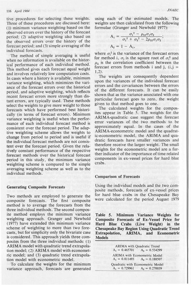
The calculated weights for the compos­ites appear in Table 5. The weights for the ARIMA-quadratic case suggest the forecast error variances of the two methods to be approximately equal. In the cases of the ARIMA-econometric model and the quadrat­ic-econometric model, the ARIMA and qua­dratic forecasts have smaller variances and therefore receive the larger weight. The small weights for the econometric model are a fur­ther indicator of the importance of time related components in ex-vessel prices for hard blue crabs.

Comparison of Forecasts

Using the individual models and the two com­posite methods, forecasts of ex-vessel prices for hard blue crabs in the Chesapeake Bay were calculated for the period August 1979

Table 5. Minimum Variance Weights for Composite Forecasts of Ex-Vessel Price for Hard Blue Crabs (Live Weight) in the Chesapeake Bay Region Using Quadratic Trend Extrapolation, ARIMA, and Econometric Models

ARIMA with Quadratic Trend A. = 0.465701 A2 = 0.534299

ARIMA with Econometric Model A1 = 0.811493 A2 = 0.188507

Quadratic with Econometric Model A. = 0.729961 A2 = 0.270039

Hudson and Capps

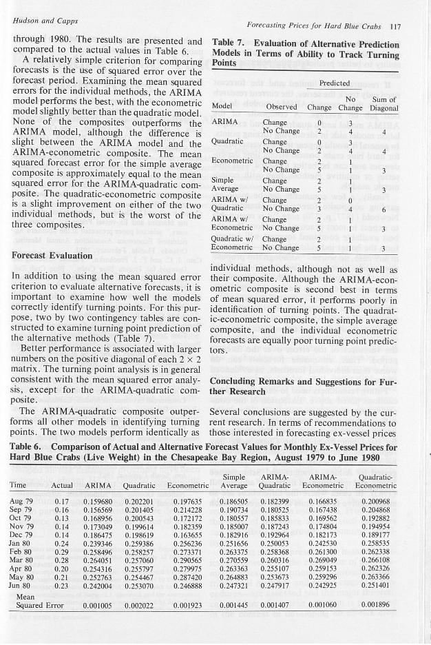
through 1980. The results are presented and compared to the actual values in Table 6.

A relatively simple criterion for comparing forecasts is the use of squared error over the forecast period. Examining the mean squared errors for the individual methods , the ARIMA model performs the best, with the econometric model slightly better than the quadratic model. None of the composites outperforms the ARIMA model, although the difference is slight between the ARIMA model and the ARIMA-econometric composite. The mean squared forecast error for the simple average composite is approximately equal to the mean squared error for the ARIMA-quadratic com­posite. The quadratic-econometric composite is a slight improvement on either of the two individual methods, but is the worst of the three composites.

Forecast Evaluation

In addition to using the mean squared error criterion to evaluate alternative forecasts, it is important to examine how well the models correctly identify turning points. For this pur­pose, two by two contingency tables are con­structed to examine turning point prediction of the alternative methods (Table 7).

Better performance is associated with larger numbers on the positive diagonal of each 2 x 2 matrix. The turning point analysis is in general

Forecasting Prices for Hard Blue Crabs 117

Table 7. Evaluation of Alternative Prediction Models in Terms of Ability to Track Turning Points

Predicted

No Sum of Model Observed Change Change Diagonal

ARIMA Change 0 3 No Change 2 4 4

Quadratic Change 0 3 No Change 2 4 4

Econometric Change 2 No Change 5 3

Simple Change 2 I Average No Change 5 I 3 ARIMA w/ Change 2 0 Quadratic No Change 3 4 6 ARIMA w/ Change 2 Econometric No Change 5 3 Quadratic w/ Change 2 Econometric No Change 5 3

individual methods, although not as well as their composite. Although the ARIMA-econ­ometric composite is second best in terms of mean squared error, it performs poorly in identification of turning points. The quadrat­ic-econometric composite, the simple average composite, and the individual econometric forecasts are equally poor turning point predic­tors.

consistent with the mean squared error analy- Concluding Remarks and Suggestions for Fur­sis, except for the ARIMA-quadratic com- ther Research posite .

The ARIMA-quadratic composite outper- Several conclusions are suggested by the cur­forms all other models in identifying turning rent research. In terms of recommendations to points. The two models perform identically as those interested in forecasting ex-vessel prices

Table 6. Comparison of Actual and Alternative Forecast Values for Monthly Ex-Vessel Prices for Hard Blue Crabs (Live Weight) in the Chesapeake Bay Region, August 1979 to June 1980

Simple ARIMA- ARIMA- Quadratic-Time Actual ARIMA Quadratic Econometric Average Quadratic Econometric Econometric

Aug 79 0.17 0.159680 0.20220 1 0. 197635 0.186505 0.182399 0.166835 0.200968 Sep 79 0. 16 0.156569 0.201405 0.214228 0.190734 0.180525 0.167438 0.204868 Oct 79 0.13 0.168956 0.200543 0. 172172 0.180557 0.185833 0.169562 0.192882 Nov 79 0.14 0.173049 0.199614 0.182359 0.185007 0.187243 0.174804 0. 194954 Dec 79 0.14 0.186475 0.198619 0.163655 0.182916 0.192964 0.182173 0.189177 Jan 80 0.24 0.239346 0.259386 0.256236 0.251656 0.250053 0.242530 0.258535 Feb 80 0.29 0.258496 0.258257 0.273371 0.263375 0.258368 0.261300 0.262338 Mar 80 0.28 0.264051 0.257060 0.290565 0.270559 0.260316 0.269049 0.266108 Apr 80 0.20 0.254316 0.255797 0.279975 0.263363 0.255107 0.259153 0.262326 May 80 0.21 0.252763 0.254467 0.287420 0.264883 0.253673 0.259296 0.263366 Jun 80 0.23 0.242004 0.253070 0.246888 0.247321 0.247917 0.242925 0.25 1401

Mean Squared Error 0.001005 0.002022 0.001923 0.001445 0.001407 0.001060 0.001896

118 April 1984

for shellfi h, the techniques of composite fore­casting should be pursued, especially if the ability to better predict turning points is desir­able.

If resources are limited and the forecast need only track the series, the current research suggests that seasonal ARIMA models do the best job on average. A composite of the ARIMA model and a quadratic trend extrapo­lation model aids in identifying turning points. In general it would appear that ex-vessel prices for hard blue crabs possess strong time depen­dencies and can be better modeled with time series or intuitive methods than with econo­metric models.

Finally , a few comments can be made re­garding composite forecasting. Granger and Newbold (1977, p. 270) note "it is reasonable to expect in most practical situations that the best available combined forecast will outper­form the better individual forecast-it cannot, in any case, do worse.'' Although this proposi­tion seems sound, it is not empirically sup­ported by the current research. The reason for the inconsistency lies in the fact that the calcu­lation of the weights is from historical data, while forecast performance is evaluated out­side the historical data. In other words, the variances of the forecast errors from which the weights are calculated may not be the same as the variances of the errors over the forecast period. Thus, composite forecasts can do worse than individual forecasts , as evidenced above.

Future researchers need to keep in mind the cautions noted above. Extension of the com­posite forecasting technique to include combi­nations of more than two forecasts may lead to better models for forecasting ex-vessel prices for hard blue crabs in the Chesapeake Bay region. Mean squared error comparisons could be made empirically using techniques sug­gested by Ashley, Granger and Schmalensee ( 1980) and implemented in Bessler and Brandt (1983). In cases where the differences are so small relative to the units of the forecast (such

JNAEC

as above), this procedure may need to be eval­uated on a benefit/cost basis.

References

Ash ley, R., C. W. J . Granger, and R. Schmalensee, "Ad­vertising and Aggregate Consumption: A Causal Analysis," Econometrica, 48( 1980): 1149-1167.

Bates, J . M. and C. W. J. Granger, "The Combination of Forecasts," Operations Research Quarterly, 6(1969):451-468.

Bessler, D. A. and J. A. Brandt, " Forecasting Livestock Prices With Individual and Composite Methods ," Applied Economics , 13(1981):513-522.

Box , G. E. P. and G. M. Jenkins, Time Series Analysis: Forecasting and Control , Holden-Day , San Fran­cisco , 1972.

Capps, Jr., 0. and L. Shabman, " Determinants of Market­ing Margins and Ex-vessel Prices for Virginia Oy­sters," selected paper presented at the Southern Ag­ricultural Economics Association Annual Meeting , Orlando , Florida, February , !982.

Cato , J. C. and F. J. Prochaska, "Factors Affecting the Demand for Florida Blue Crabs ," Blue Crab Col­loquium, Gulf States Marine Fisheries Committee, 1980.

Chui , Margaret Kam-Too, " Ex-vessel Demand by Size fo r the Gulf Shrimp," unpublished M.S. thesis, Texas A&M University, August !980.

Granger, C. W. J. and P. Newbold, Forecasting Economic Time Series , Academic Press, New York , 1977.

Prochaska, Fred J. , "Prices, Marketing Margins , and Structural Changes in the King Mackerel System ," South ern Journal of Agricultural Economics ( 1978): 105-109.

Rausser , G. C. and R. E. Just , "Agricultural Commodity Price Forecasting Accuracy: Futures Markets Versus Commercial Econometric Models , California Agricul­tural Experiment Station Working Paper No. 66, pr~ sented at Futures Market Research Symposium, Chicago, Illinois, 1979.

Rhodes, Raymond J ., " Ex-vessel Price Trends in the United States Blue Crab Fishery," unpublished pa­per, Division of Marine Resources South Carolina Wildlife and Marine Resources Department, Charles­ton , South Carolina, 1981.

Shellfish Market Review, U.S. Department of Commerce, National Oceanic and Atmospheric Administration, National Marine Fisheries Servi <::e.