Kansas State University Libraries Kansas State University Libraries

New Prairie Press New Prairie Press

Conference on Applied Statistics in Agriculture 1989 - 1st Annual Conference Proceedings

FORECASTING CORN EAR WEIGHT USING SURFACE AREA AND FORECASTING CORN EAR WEIGHT USING SURFACE AREA AND

VOLUME MEASUREMENTS: A PRELIMINARY REPORT VOLUME MEASUREMENTS: A PRELIMINARY REPORT

Fatu Bigsby

Follow this and additional works at: https://newprairiepress.org/agstatconference

Part of the Agriculture Commons, and the Applied Statistics Commons

This work is licensed under a Creative Commons Attribution-Noncommercial-No Derivative Works 4.0 License.

Recommended Citation Recommended Citation Bigsby, Fatu (1989). "FORECASTING CORN EAR WEIGHT USING SURFACE AREA AND VOLUME MEASUREMENTS: A PRELIMINARY REPORT," Conference on Applied Statistics in Agriculture. https://doi.org/10.4148/2475-7772.1463

This is brought to you for free and open access by the Conferences at New Prairie Press. It has been accepted for inclusion in Conference on Applied Statistics in Agriculture by an authorized administrator of New Prairie Press. For more information, please contact cads@k-state.edu.

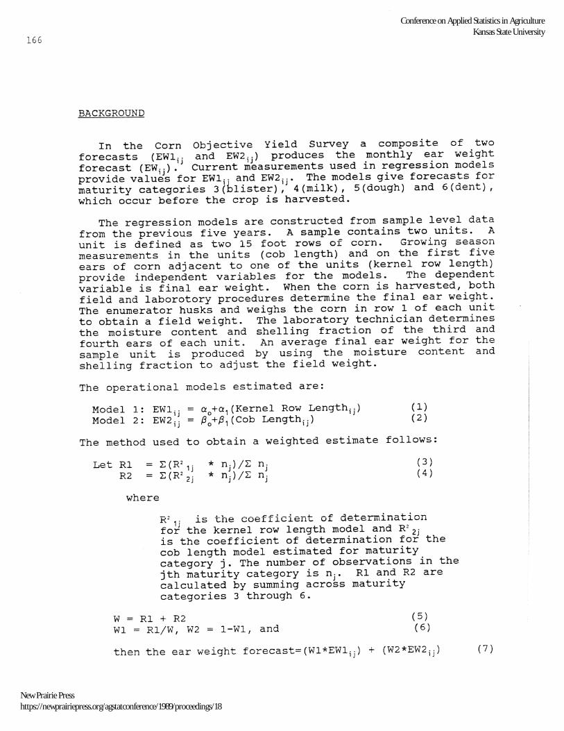
FORECASTING CORN EAR WEIGHT USING SURFACE AREA AND VOLUME MEASUREMENTS: A PRELIMINARY REPORT

Fatu Bigsby National Agricultural statistics Service

U.s. Department of Agriculture Washington, D.C.

ABSTRACT

Data from the Corn Ear Weight Study were used to analyze the forecast performance of models estimated using surface area and volune measurements to predict corn ear weight. Two models based on research measurements were compared to models estimated using the operational procedures from the Corn Objective Yield Survey. Research and operational models were estimated both within and across years using data from the 1986 and 1987 Michigan Corn Ear Weight Study. Results show that research models based on surface area and volune measurements have mean square errors that are 32 to 52 percent lower than models estimated using the operational procedure. The differences between forecast errors of the research and operational models are statistically significant.

KEY WORDS: corn; objective yield; ear weight; volune; surface area; forecast error.

1. INTRODUCTION

The National Agricultural statistics Service (NASS) uses the Corn Objective yield Survey to forecast corn yield, acreage and production [4]. In the Objective yield Survey, gross yield is defined as the number of corn ears times the average final ear weight. Net yield, estimated at the state level, is gross yield minus estimated harvest loss. The Corn Ear Weight Study examines one component used to determine yield, specifically, the ear weight.

The purpose of the Corn Ear Weight Study is to develop a more accurate ear weight estimator using surface area and/or volume measurements of the corn ear in addition to the length measure­ments made in the operational program. Surface area and volume measurements not only have a potential of producing superior forecasts during normal conditions, but especially during drought years. Using ear length alone may not accurately forecast ear weight because of a reduction in the total ear size.

The first part of the paper gives the background of the study. Subsequent sections give the methodology used to derive and validate the forecast models. Results obtained from these methods using 1986 and 1987 data for Michigan are also given.

165

Conference on Applied Statistics in AgricultureKansas State University

New Prairie Presshttps://newprairiepress.org/agstatconference/1989/proceedings/18

166

BACKGROUND

In the Corn Objective Yield Survey a composite of two forecasts (EWlij and EW2ij) produces the monthly ear weight forecast (EW jj ). Current measurements used in regression models provide values for EWl j " and EW2 jj • The models give forecasts for maturity categories 3 (hlister), 4 (milk) , 5 (dough) and 6 (dent) , which occur before the crop is harvested.

The regression models are constructed from sample level data from the previous five years. A sample contains two units. A unit is defined as two 15 foot rows of corn. Growing season measurements in the units (cob length) and on the first five ears of corn adjacent to one of the units (kernel row length) provide independent variables for the models. The dependent variable is final ear weight. When the corn is harvested, both field and laborotory procedures determine the final ear weight. The enumerator husks and weighs the corn in row 1 of each unit to obtain a field weight. The laboratory technician determines the moisture content and shelling fraction of the third and fourth ears of each unit. An average final ear weight for the sample unit is produced by using the moisture content and shelling fraction to adjust the field weight.

The operational models estimated are:

Model 1: EWl ij = ao+a, (Kernel Row Length jj )

Model 2: EW2ij = f3 o+f3,(Cob Lengthij) ( 1) (2)

The method used to obtain a weighted estimate follows:

Let Rl R2

= L(R2," = L (R2 2~

(3) (4)

where

.1:<: 1j is the coefficient of determination for the kernel row length model and R2 2j is the coefficient of determination for the cob length model estimated for maturity category j. The number of observations in the jth maturity category is n j • Rl and R2 are calculated by summing across maturity categories 3 through 6.

W = Rl + R2 WI = Rl/W, W2 = I-WI, and

(5) (6)

then the ear weight forecast=(Wl*EWlij) + (W2*EW2 i ) (7)

Conference on Applied Statistics in AgricultureKansas State University

New Prairie Presshttps://newprairiepress.org/agstatconference/1989/proceedings/18

Kernel row length (1) and cob length (2) were chosen by prior NASS researchers because of their obvious relationship to ear weight.

Ronald Steele initiated the Corn Ear Weight study in 1985 [3]. He modeled the relationship of individual surface area and volume measurements on 78 ears of corn to their final ear weight. The ears were obtained from two purposefully selected fields in Nebraska. Analyses of the Nebraska data showed that models derived from surface area and volume measurements were promising. The Corn Ear Weight Study began formally in 1986 in Michigan. The study differs from the Nebraska analysis in that a probability sample is used to forecast ear weight at the sample level. The Michigan state statistical Office staff collected the data. The author conducted the analyses using SAS[2].

2 • METHODOLOGY

Data Collection

Data collection for the study continued for two consecutive years during the Corn Objective yield Survey in Michigan (5]. September 1 and October 1 were the survey periods for data collection. The maturity categories for the modeling effort were 4 (milk), 5 (dough) and 6 (dent). Maturity category 3 (blister) was excluded from the study because of the assumption that size of the corn ear, at this stage of maturity, was not large enough to show a significant relationship to the final ear weight.

The enumerators made three measurements on ears in row 1 of the first and second sample units with a vernier caliper. The measurements were: Length of the kernel row, diameter of the cob two inches from the tip, and diameter of the cob one inch from the butt.

Research Models

The ear weight model defined using Least Squares is

Yi = f3 0 + f3 1X , + f32X2 + e (8)

where,

Yi=final ear weight for the ith sample field, X1 or X2 = a surface area or volume or length variable e i = the difference between final ear weight

and the estimate produced by the model.

167

Conference on Applied Statistics in AgricultureKansas State University

New Prairie Presshttps://newprairiepress.org/agstatconference/1989/proceedings/18

168

Although ear length variables were available for inclusion in the research models, the models were forced to contain a surface area and/or volume variable. The maximum number of independent variables in a model was restricted to two because the use of more than two independent variables did not improve the forecasting ability of the models. The models were estimated across maturity categories.

The research models estimated were:

Model R1: Ear Weight 1" = Q + Q S 1 + /3 BT + e ,.., 0 ,.., i i 2 i i

Model R2: Ear weight; = /3 0 + /3,V2i + /3 2BD i + e i

Where,

Sl=(Husk Length) * Butt Diameter BT= Butt Diameter * Tip Diameter V2=(Husk Length* Tip Diameter2)/4 * ff

BD= Butt Diameter

(9)

(10)

The research models were selected because they had lower regression mean square errors and higher R2 ,s than other models that were examined.

The operational model provided a benchmark for assessing performance of a research model. The author estimated the operational model using two methods. The background section of this paper gave the first method (1) (7) . The exception occurs in calculating R1 and R2 in (3) and (4). R2 's for the kernel row length (KL) and husk length (HL) models result from fitting the models across all maturity categories. The operational model estimated using this method is referred to as model ° S.

The second method estimates the relationship of the two operational independent variables (kernel row length and cob length) to the dependent variable in the same model. Estimation of the operational model using this method produces a more meaningful comparison of the operational and research models because the research model defined in (8) is estimated in this manner. O_J, the operational model estimated using the second method is defined as

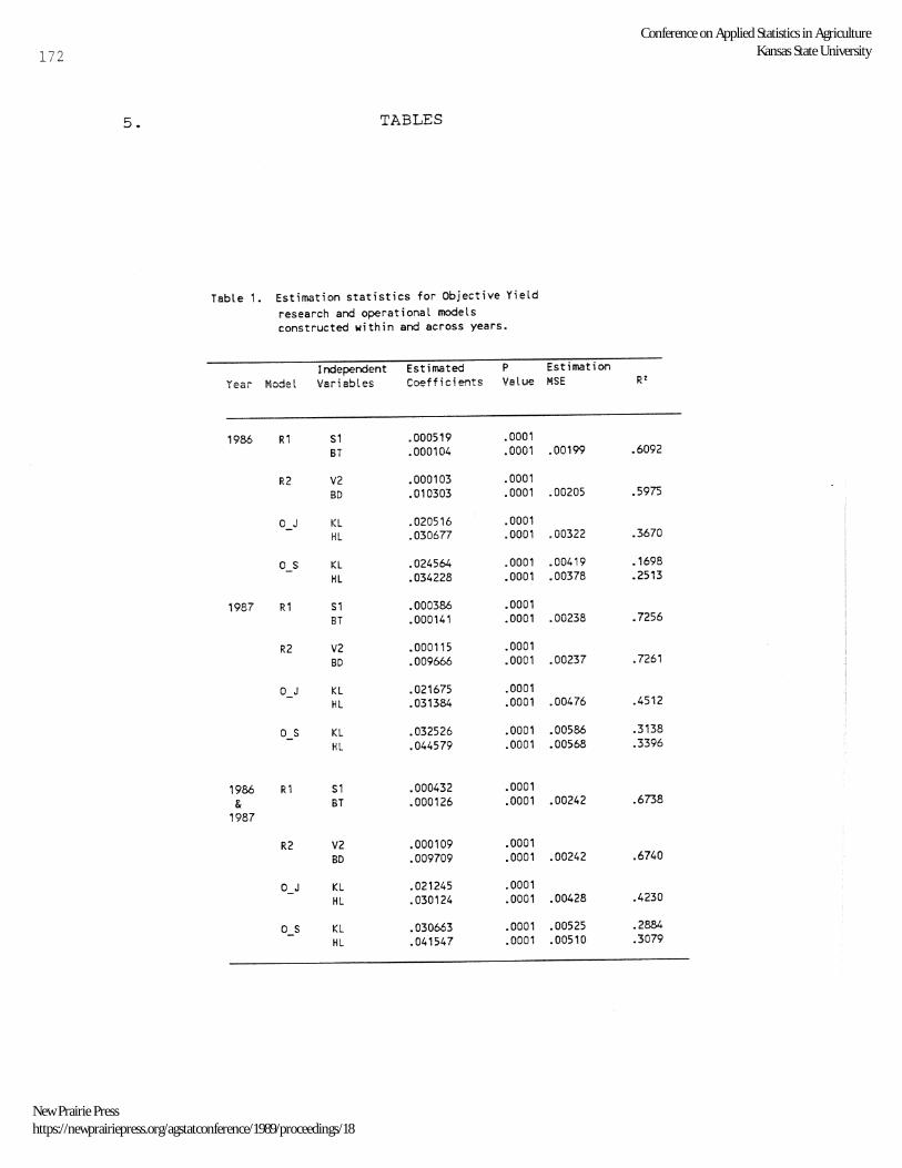
Table 1 contains independent variables, estimated slope coefficients, P values, estimation mean square errors (MSEs) and R2 s for the research and operational models. It shows that parameters estimated for variables in all models, research and operational, have observed significance levels equal to .0001. Estimation MSEs of the research models are smaller than those of

Conference on Applied Statistics in AgricultureKansas State University

New Prairie Presshttps://newprairiepress.org/agstatconference/1989/proceedings/18

the operational models and R2 s of the research models are almost twice as high as those of the operational models. Both these measures of model efficiency confirm the improved properties of the research models over the operational models.

3. VALIDATION OF RESEARCH MODELS

Validation gives an indication of the forecasting ability of a model by determining how the model performs using data other than that used for its estimation. The 1987 data was used for validating the 1986 models and vice versa. Data for validating the models based on the combined data for 1986 and 1987 included a random sample of one-half of the observations from September. These earlier observations provided a better test of the ability of the models to forecast than do the October observations.

The validation procedure used mean square errors to compare the performance of two or more models. The mean square error was computed from the forecast error. The forecast error is the difference between the final ear weight for the ith sample field and the ear weight forecast for the same field. Table 2 gives the MSEs of the research and operational models and shows that both research models have smaller mean square errors than the operational models for all validation data. Furthermore, Table 2 shows that the reduction in MSE when forecasting with the research model is at least 32 percent.

Since the MSEs indicated differences in the abilities of the models to forecast ear weight, conducting a one-way analysis of variance (ANOVA) determined if the differences were statisti­cally significant.

A. one-way ANOVA defined the following model:

Where,

y .. 1 J

(12)

= the absolute value of the forecast error for the ith sample field and jth model,

= the overall mean, = the effect of of the forecast error for

the jth model, and = the deviation of (J.J.. + 'r j ) from Yij •

The absolute value of the forecast error was considered a response because of interest in the absolute deviation of the forecast from the final ear weight. The analysis of variance used the model in (12) to test the following hypotheses:

169 Conference on Applied Statistics in Agriculture

Kansas State University

New Prairie Presshttps://newprairiepress.org/agstatconference/1989/proceedings/18

170

Ho: 1, = 12 = 13 = ... 1 Ie' k = the number of models Ha: not all 1 j 'S are zero, j = 1,2, ... ,k

The test chosen was nonparametric since the statistical distribution of the absolute values of the forecast errors was unkown. The test statistic [1] used was:

F = R

where,

Rj

R . j

nj

n

=

=

=

=

= rank of absolute value of the ith forecast error for the jth model when forecast errors for all models are ranked jointly from 1 to n,

sum of the ranks for model j's forecasts,

average rank for model j's forecasts,

the number of observations for model j, and total number of observations.

(13)

The numerator in FR (13) represents differences between ranks of the k models and the denominator represents differences within ranks of the kth model. If the null hypothesis is true and the forecast effect is essentially zero, then FR will be small. The test rejects Ho for values of F~ larger than the (1-a; k-1,n-k) percentile of the F distrlbution. The null hypothesis is rejected for observed significance levels (P values) smaller than or equal to 0.10.

Table 3 gives the nonparametric ANOVA results. For each type of validation data, two types of comparisons were made. The first comparison examined differences among forecast error means of research model R1 (9) and operational models o_5 (7) and O_J (11) . Likewise, the second comparison examined differences among forecast error means of research model R2 (10) and operational models 0 S (7) and 0 J (11). The last column of the table shows observed significance levels for each type of validation data. The observed levels are all less than .02 which leads to rejection of the null hypothesis that the forecast effect is essentially zero.

Although Table 3 shows that at least two of the three models in each type of comparison have significantly different forecast errors, the table does not show which two are different. The Tukey multiple comparison procedure determined which forecasts were different from each other and controled the experimentwise

Conference on Applied Statistics in AgricultureKansas State University

New Prairie Presshttps://newprairiepress.org/agstatconference/1989/proceedings/18

error rate at .10. The procedure was performed on ranks of absolute values of the forecast errors. Confidence intervals were constructed simultaneously for all pairs of forecasts.

The interval

D - Ts(D) < ~j - ~j' <_ D + Ts(D) (14)

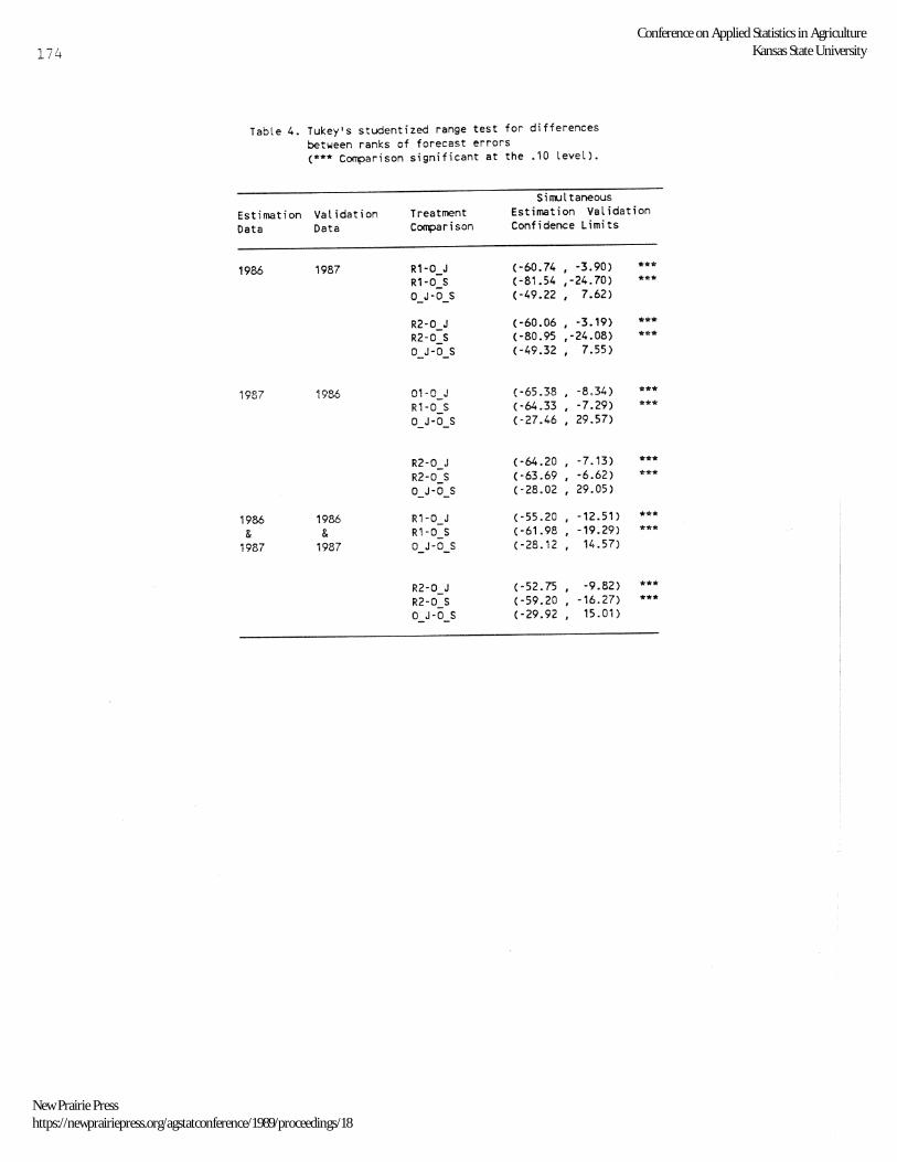
determined the difference between errors of the jth and jth' forecasts. D is the difference between average ranks of the errors, s is the standard deviation of D, and T is the (l-a, k, n-k) percentile of the studentized range distribution. Only if the interval constructed in (14) contains zero will the forecast errors be statistically the same. otherwise the forecast errors are different. Table 4 gives simUltaneous upper and lower confidence levels constructed for the validation data sets. The table shows that differences between forecast errors of the research and operational models are significant.

4. SUMMARY

Data from the 1986 and the 1987 Michigan Corn Ear weight Study were used to estimate ear weight models employing surface area or volume measurements as independent variables. These models had mean square errors that are 32 to 52 percent lower than those for operational models for the 1986 and 1987 val idation data. Mean square errors of the research models estimated using data for both years were 44 to 48 percent lower than those of the operational models for the same period. Tests of statistical hypotheses and multiple comparison procedures conducted suggested that differences between forecast errors of the research and operational models were significant.

The Corn Ear Weight Study continued in Michigan in 1988 and was also expanded to Missouri to evaluate the performance of the surface area and volumes models in an environment that is more drought prone than Michigan. Results of 1988 data will be available at a later date.

171 Conference on Applied Statistics in Agriculture

Kansas State University

New Prairie Presshttps://newprairiepress.org/agstatconference/1989/proceedings/18

172

5. TABLES

Table'. Estimation statistics for Objective Yield research and operational models constructed within and across years.

Independent Estimated P Estimation Year Model Variables Coefficients Value HSE R'

1986 R1 S1 .000519 .0001 BT .000104 .0001 .00199 .6092

R2 V2 .000103 .0001 SO .010303 .0001 .00205 .5975

O_J KL .020516 .0001 HL .030677 .0001 .00322 .3670

° 5 ICL .024564 .0001 .00419 .1698 HL .034228 .0001 .00378 .2513

1987 R1 51 .000386 .0001 ST .000141 .0001 .00238 .7256

R2 V2 .000115 .0001 BD .009666 .0001 .00237 .7261

o J KL .021675 .0001 HL .031384 .0001 .00476 .4512

0_5 KL .032526 .0001 .00586 .3138 HL .044579 .0001 .00568 .3396

1986 Rl 51 .000432 .0001 & BT .000126 .0001 .00242 .6738

1987

R2 V2 .000109 .0001 BO .009709 .0001 .00242 .6740

° J KL .021245 .0001 HL .030124 .0001 .00428 .4230

0_5 KL .030663 .0001 .00525 .2884 HL .041547 .0001 .00510 .3079

Conference on Applied Statistics in AgricultureKansas State University

New Prairie Presshttps://newprairiepress.org/agstatconference/1989/proceedings/18

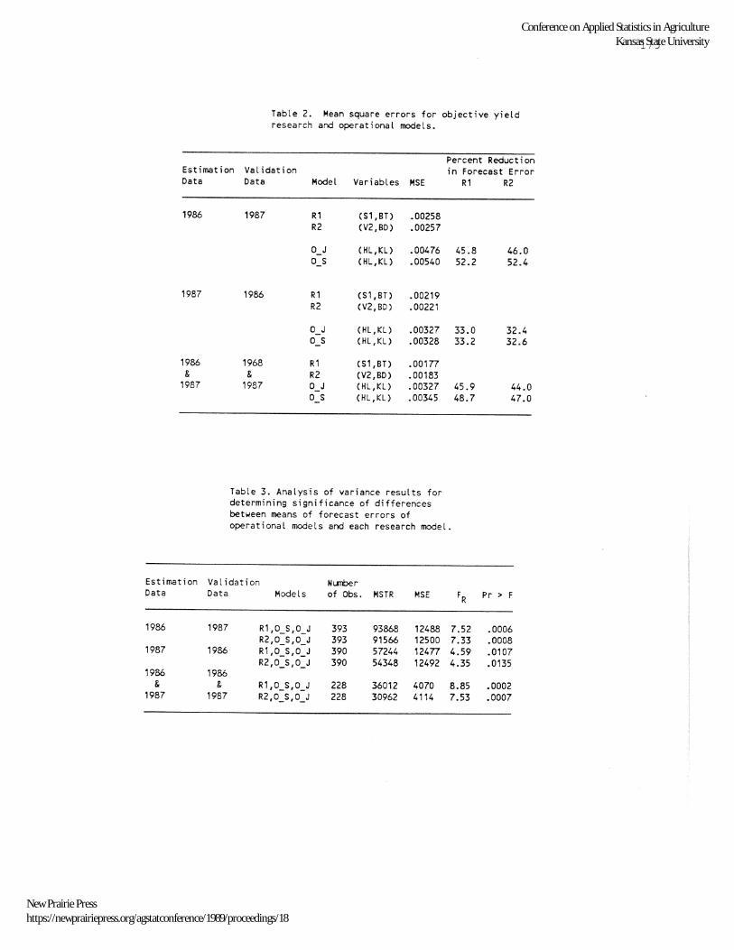
Table 2. Mean square errors for objective yield research and operational models.

Percent Reduction Estimation Validation in Forecast Error Data

1986

1987

1986 &

1987

Estimation Data

1986

1987

1986 &

1987

Data Model Variables M5E

1987 Rl (51, BT) .00258 R2 (V2,BD) .00257

O_J (Hl,KL) .00476 0_5 (Hl,KL) .00540

1986 R1 (S1,BT) .00219 R2 (V2,BD) .00221

O_J (Hl,Kl) .00327 0_5 (Hl,KL) .00328

1968 Rl (51,BT) .00177 & R2 (V2,BD) .00183

1987 O_J (Hl,Kl) .00327 0_5 (HL,KL) .00345

Table 3. Analysis of variance results for determining significance of differences between means of forecast errors of operational models and each research model.

Val idation Nl.JTlber Data Models of Obs. MSTR M5E

1987 Rl,O_5,O_J 393 93868 12488 R2,O_S,O_J 393 91566 12500

1986 Rl,O_5,O_J 390 57244 12477 R2,O_5,O_J 390 54348 12492

1986 & R1,O_5,O_J 228 36012 4070

1987 R2,O_5,O_J 228 30962 4114

Rl R2

45.8 46.0 52.2 52.4

33.0 32.4 33.2 32.6

45.9 44.0 48.7 47.0

FR Pr > F

7.52 .0006 7.33 .0008 4.59 .0107 4.35 .0135

8.85 .0002 7.53 .0007

173 Conference on Applied Statistics in Agriculture

Kansas State University

New Prairie Presshttps://newprairiepress.org/agstatconference/1989/proceedings/18

174

Table 4. Tukey's studentized range test for differences betloleen ranks of forecast errors (*** Comparison significant at the .10 level).

SilTlJltaneous Estimation Val idation Treatment Estimation Val idation Data Data Comparison Confidence Limits

1986 1987 R1-0_J (-60.74 -3.90) *** , R1-0_S (-81.54 ,-24.70) *** O_J-O_S (-49.22 , 7.62)

R2-0_J (-60.06 -3.19) *"'* , R2-0_S ( ·80.95 ,-24.08) "',.* O_J-O_S (-49.32 . 7.55)

1987 1986 01-0_J C -65 .38 -8.34) "** R1-0_S (-64.33 -7.29) *"'* O_J-O_S (-27.46 , 29.57)

R2-0_J (-64.20 -7.13) *** R2-0_S (-63.69 -6.62) "'** O_J-O_S (-28.02 , 29.05)

1986 1986 R1-0_J (-55.20 -12.51 ) *** 8. & R1-0_S (-61.98 -19.29) *"*

1987 1987 O_J-O_S (-28. '2 , 14.57)

R2-0_J (-52.75 -9.82) *** R2-0_S (-59.20 -16.27) *** ° J-O S (-29.92 , 15.01)

Conference on Applied Statistics in AgricultureKansas State University

New Prairie Presshttps://newprairiepress.org/agstatconference/1989/proceedings/18

REFERENCES

1. Conover, W.J., and Ronald L. Iman. Rank Transfor­mations as a Bridge Between Parametric and Non­parametric statistics, The American Statistician, August 1981, Vol. 35, No.3.

2. SAS Institute Inc. SAS/STAT Guide for Personal Computers, Version 6 Edition. Cary, NC: SAS Institute inc., 1985

3. Steele, Ronald J., 1985. Preliminary Investigation For An Improved Corn Grain Weight Forecast Model, Unpublished.

4. U.S. Department of Agriculture, 1987 Corn Objective Yield Survey: Supervising & Editing Manual, National Agricultural Statistics Service, Washington, D.C., 1987

5. U.S. Department of Agriculture, 1987 Michigan Corn Research Study, National Agricultural statistic Service, Washington, D.C., 1987

175 Conference on Applied Statistics in Agriculture

Kansas State University

New Prairie Presshttps://newprairiepress.org/agstatconference/1989/proceedings/18