Forecasting Cinema Attendance at the Movie Show Level

73

Business Systems Research | Vol. 11 No. 1 |2020

Forecasting Cinema Attendance at the

Movie Show Level: Evidence from Poland

Paweł Baranowski

Department of Econometrics, Faculty of Economics and Sociology, University

of Łódź, Łódź, Poland

Karol Korczak, Jarosław Zając

Department of Computer Science in Economics, Faculty of Economics and

Sociology, University of Łódź, Łódź, Poland

Abstract

Background: Cinema programmes are set in advance (usually with a weekly

frequency), which motivates us to investigate the short-term forecasting of

attendance. In the literature on the cinema industry, the issue of attendance

forecasting has gained less research attention compared to modelling the aggregate

performance of movies. Furthermore, unlike most existing studies, we use data on

attendance at the individual show level (179,103 shows) rather than aggregate box

office sales. Objectives: In the paper, we evaluate short-term forecasting models of

cinema attendance. The main purpose of the study is to find the factors that are useful

in forecasting cinema attendance at the individual show level (i.e., the number of

tickets sold for a particular movie, time and cinema). Methods/Approach: We apply

several linear regression models, estimated for each recursive sample, to produce

one-week ahead forecasts of the attendance. We then rank the models based on

the out-of-sample fit. Results: The results show that the best performing models are

those that include cinema- and region-specific variables, in addition to movie

parameters (e.g., genre, age classification) or title popularity. Conclusions: Regression

models using a wide set of variables (cinema- and region-specific variables, movie

features, title popularity) may be successfully applied for predicting individual cinema

shows attendance in Poland.

Keywords: cinema attendance, movie, IMDb, forecasting, data mining, decision

support models

JEL classification: L82, C53, D81, Z11

Paper type: Research article

Received: Jun 7, 2019

Accepted: Dec 12, 2019

Citation: Baranowski, P., Korczak, K., Zając, J. (2020), “Forecasting Cinema

Attendance at the Movie Show Level: Evidence from Poland”, Business Systems

Research, Vol. 11 No. 1, pp. 73-88.

DOI: 10.2478/bsrj-2020-0006

74


Introduction Participating in cultural events is an important determinant of an individual’s quality of

life (e.g. Casson, 2006; Weziak-Bialowolska et al., 2018). In this paper, we focus on a

considerable segment of cultural expenditures: the cinema industry. Forecasting

cinema attendance may be crucial in cinema management for several reasons.

Firstly, we observe the long-run decline in cinema ticket sales. This phenomenon is

influenced by, among others, the development of television, DVD and other home

video products (Cameron, 1988), piracy (Li, 2012) or video streaming (Wayne, 2018).

It is important though to verify empirically the evidence on the factors driving cinema

attendance. Secondly, as with many other cultural events, cinema programmes are

set in advance. Cinema operators usually rely on their own intuition and experience

when planning a cinema repertoire. Such forecasts, based on human judgment,

maybe a subject of significant bias and are typically outperformed by econometric

modelling (Makridakis et al., 2009). Thirdly, given the fact that cinema operators often

apply a bundling strategy, higher cinema attendance also contributes to sales of

complementary products, such as snacks or beverages (this phenomenon is

especially evident in large cinemas, e.g. Doury, 2001; Dewenter and Westermann,

2005) as well as revenues from advertising.

The literature on forecasting consumer demand or behavioural patterns indicates

not only to identify new determinants but also to combine those related to the

product’s features and its’ reputation, location of the business or macroeconomic

situation. Applications in the field of economics and business include, among others,

predicting the credit risk (Sztaudynger, 2018), modelling credit card usage (Goczek

and Witkowski, 2016) and travel behaviour (Klinger and Lanzendorf, 2016). However,

in accordance with our best knowledge, the issue of modelling and forecasting

cinema attendance has not been fully researched in the field yet. When considering

the broader scope of studies on leisure services, up to this point multilevel models are

limited to tourism research (Jeffrey and Barden, 2001; Yang and Cai, 2016). In addition,

recent contributions to the field of business forecasting also include data gathered

from social media (e.g. Bukovina, 2016; Yuan et al., 2018). We partially address this

issue by considering variables from the Internet Movie Database (IMDb). Finally, a

number of papers suggest a higher level of uncertainty after the Global Financial Crisis

(Bloom 2014; Moore 2017). In such a volatile environment, there is an even greater

need for forecasting and business planning.

Therefore, we attempt to answer the question: which variables are useful in the

short-term forecasting of cinema attendance at the individual show level? We use a

dataset derived from a large cinema network in Poland that covered 19 months of

sales history. Our study may be perceived as unique due to dataset structure that

includes the attendance at individual shows (characterised by the date and time,

location of the cinema and movie title), while prior studies (e.g., Hand, 2002; Walls,

2005; Collins et al., 2009) rely on aggregate box-office sales for titles or cinemas. Within

the presented approach, it is possible to plan not only the repertoire (e.g. Marshall et

al., 2013) but also the showing time or distribution across cinemas.

The aim of the paper is to build short-term forecasting models of cinema

attendance and to examine which factors improve predictive power for forecasting

cinema attendance at the individual show level. In order to complete research

objectives, four groups of factors were firstly specified and further 16 regression models

with different variables sets (cinema-specific, region-specific, movie parameters and

title popularity) were compared.

The paper has the following structure. Firstly, an overview of the literature in the field

of modelling and forecasting phenomena in the cinema industry was presented.

75


Secondly, the characteristics of data and methods were described. Thirdly, the errors

of the out-of-sample forecasts were analysed. The research procedure included also

robustness checks. Finally, the discussion and concluding remarks were presented.

Literature review Modelling and forecasting phenomena in the cinema industry have been present in

the literature for a long time. The first strand of the literature focuses on aggregate

cinema ticket sales, including notable decreases in cinema attendance that were

observed in the 1960s as well as the 1980s. These studies concluded that the drop in

cinema attendance was mainly caused by the development of television, the arrival

of home video formats like VHS, demographic factors and lower quality of movies

(Jones 1986; Cameron, 1988; MacMillan and Smith, 2001; Pautz, 2002). Hand and

Judge (2012) showed that using the number of searches of terms related to movies or

cinemas (i.e. Google Trends data) may improve short-term forecasts of aggregate

cinema admissions.

A large amount of the literature analyses cinema attendance across movies, using

data observed at the movie level, i.e. the overall tickets sold for a movie (e.g., Walls,

2005; Marshall et al., 2013; Gmerek, 2015; Treme et al., 2018). Walls (2005) predicted

financial success during the early stages of new movies where only the parameters of

the movie itself were used for forecasting. The feature that distinguishes this study is the

inclusion of movie characteristics such as negative cost, opening screens, whether it

was a sequel, stars, genre, rating, and year of release. The results confirmed that a

robust regression model is a better tool for predicting the financial success of movies

than the often-applied least-squares regression model. In a recent study, Treme et al.

(2018) verified the dependence between variables expressing cast (in particular, the

gender of the movie’s stars) and box office performance. The model, which explained

the movies’ commercial success, included variables such as stars (number and

gender), budget, the maximum number of domestic theatres where the movie was

played, major distributors (dummy variables), genre, different ratings (ratings from the

Motion Picture Association of America (MPAA), critics, viewers), decade, and release

date. The results of this study showed that having at least one star in the cast increases

the movie’s revenue by 10%. What is more, this revenue grows when there are male

stars in the cast. Marshall et al. (2013) focused on a system for forecasting movie

attendance, using weekly attendance data across the movies. This study is close to

ours in terms of the set of independent variables, including genre, country of origin,

age rating, movie popularity, whether the film was a sequel and seasonality. Variables

related to movie awards and finance (e.g. budget, public subsidies) are also included

in cinema attendance analysis (Nelson et al., 2001; Jansen, 2005; Feng, 2017). Recent

studies focus on the impact of movie popularity on social media (Treme and

VanDerPloeg, 2014, Ding et al., 2017) or word-of-mouth reviews (Dellarocas et al.,

2007; Duan and Whinston, 2008; Craig et al., 2015) on box-office performance.

Few papers analyse the cinema industry at the cinema-level. Hand (2002) applied

univariate time series models (including autoregressive moving average – ARMA) to

predict cinema admissions. Hand concluded that even if individual movie admissions

are not predictable (De Vany and Walls, 1999), we could predict attendance at the

cinema level. Collins et al. (2009) analysed a conventionality index—a measure of

cinema programme differentiation. However, while the study examined the impact of

several factors (size of the market, age structure, per capita income, and a dummy

variable for multiplexes) on the conventionality, it ignored attendance.

The propensity that an individual goes to the cinema is separate and at the same

timeless related issue in the literature (Collins and Hand, 2005; Cameron, 1999;

76


Dewenter and Westermann, 2005; Sisto and Zanola, 2007). These studies mostly use the

characteristics of the individual or the household, which are not accessible in our study

(typically the viewer is not identified by the cinema). However, we proxy these factors

by the average salary in the region where the cinema is located and typically the

customer has the place of residence (Goczek and Witkowski, 2016).

It should also be underlined that the cinema industry is similar to other branches of

the entertainment industry. In the literature, we can find studies that have been

devoted to forecasting attendance, for example in a museum (Cuffe, 2018). The

results of Cuffe’s study show that rainfall during certain hours of the day can

significantly affect museum attendance.

Data and methods The paper examines which of the variables is useful in predicting cinema attendance

in a one-week time horizon. Thus, we compare the forecasts obtained from

multivariate regression models, including different sets of independent variables.

Before we describe the forecasting method and the models, let us introduce the

sources and properties of the data.

We build on the dataset at the individual show level, where a single observation

denotes the number of tickets sold for a particular cinema screen at a given time.

Compared to the most popular movie-level data, our dataset also distinguishes the

time and the place of the movie show. These data are obtained from a large cinema

network functioning in Poland (henceforth referred to as the Operator). The sample

used in this study covers 25 cinemas (located in 24 Polish cities) and the period from

October 2016 to March 2018. During that period, the Operator exhibited 259 unique

titles. Overall, the dataset contains 179,103 observations, of which the last 16 weeks

were used for forecasts’ verification (51,980 out-of-sample observations—i.e., 29% of

the full sample). In this study, we include the opening week (the week that the

particular movie is released) from the dataset. This approach is motivated twofold.

Firstly, the evidence from studies analysing box-office performance of movies suggest

that attendance during the first week is specific, determined by the promotion, social

media news or the sentiment of movie reviews (Ainslie, 2005; Sharda and Delen, 2006;

Yu et al., 2012) and should be modelled separately from subsequent weeks. Secondly,

our model relies on data that are not available (or hardly achievable) before the

movie release (e.g. movie popularity from IMDb).

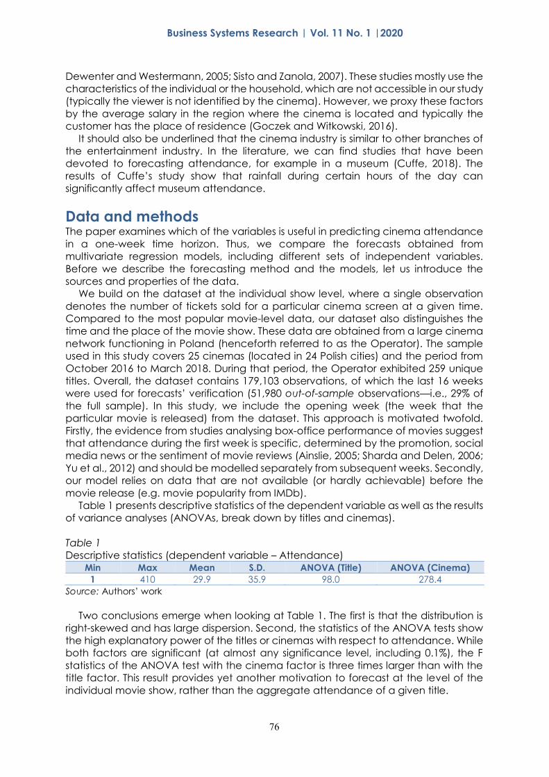
Table 1 presents descriptive statistics of the dependent variable as well as the results

of variance analyses (ANOVAs, break down by titles and cinemas).

Table 1

Descriptive statistics (dependent variable – Attendance) Min Max Mean S.D. ANOVA (Title) ANOVA (Cinema)

1 410 29.9 35.9 98.0 278.4

Source: Authors’ work

Two conclusions emerge when looking at Table 1. The first is that the distribution is

right-skewed and has large dispersion. Second, the statistics of the ANOVA tests show

the high explanatory power of the titles or cinemas with respect to attendance. While

both factors are significant (at almost any significance level, including 0.1%), the F

statistics of the ANOVA test with the cinema factor is three times larger than with the

title factor. This result provides yet another motivation to forecast at the level of the

individual movie show, rather than the aggregate attendance of a given title.

77


In general, we examine the role of four groups of variables. We group variables that

provide similar information about cinema characteristics, movie characteristics and its

popularity, and the macroeconomic conditions of the region. A similar approach was

previously proposed, among others, by Hofmann-Stölting et al. (2017) and Wu et al.

(2018). In these studies, we can find variables reflecting product quality, pricing

factors, cinema configurations, competition, advertising, and selected external

factors. Our approach is comprehensive in the sense that we include factors

grounded in the economy, entertainment industry economy as well as cultural events

planning. In addition to listing the variables, we provide motivation for using the

variables in the study.

o Cinema-specific – features of the cinema, such as the number of screens in the

cinema (Screens) and capacity—number of seats (Seats), collected from the

Operator’s database. Such features serve here as a proxy for the reputation of a

particular cinema (e.g., Collins et al., 2009), which attracts audience irrespective

of other factors,

o Region-specific – average monthly earnings in each NUTS-4 region (RegionWage)

and population in each NUTS-3 region (RegionPopul), collected from the Polish

Statistical Office – Local Data Bank (https://bdl.stat.gov.pl/BDL/start). Average

earnings represent income, which is typically considered when modelling demand

and the population expresses the market size. These variables, expressing the

characteristics of the place of residence, were used also when modelling the

propensity for holding a payment or credit card (e.g. Goczek and Witkowski, 2016).

The data on earnings and population are available with quarterly and bi-annual

frequency, respectively,

o Movie parameters – running time in minutes (MovieLength), genre (9 dummy

variables, representing 10 genres present in the dataset), country of the producer

(2 dummy variables, representing Poland and the United States), dummy for 3D

sound (Sound), dummy for sequels (Sequel), number of stars from top the 20 stars

according to the IMDb (Stars20), dummy for movies targeted at small children

(Childr), age classification, taking values 0, 6, 7, 10, 12, 13, 15, 18 (AgeClass), age

of the movie in years (year it was shown minus the year of release; MovieAge). Such

variables describe the final product being offered and play a key role in the choice

of the movie; they are routinely used in the literature on modelling and forecasting

a movie’s attendance or revenue (e.g., Litman 1983; Walls, 2005),

o Title popularity – average rating (RatingIMDB) and a number of votes (VotesIMDB)

collected from IMDb. Including these variables in the regression is motivated by

studies on the relationship between the influence of popularity (e.g., the number

of visits to internet auctions sites) and customer feedback on sales (e.g., Duan and

Whinston, 2008; Baranowski et al., 2018).

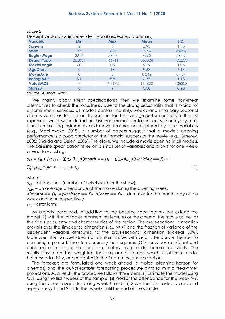
Table 2 presents summary statistics of the independent, continuous variables used

in the study. The results presented in Table 2 show that the sample is diverse. More

specifically, the sample covers different types of cinemas (i.e. from 2 to 8 screens, and

the screens ranging from 57 to 483 seats). The sample is also diversified across the

regions—both with respect to income (wage) per capita and population. The

Operator exhibited mostly new movies (shown during the first year of release), though

the movies varied greatly in popularity indicators (number of votes and rating from

IMDb).

78


Table 2

Descriptive statistics (independent variables, except dummies) Variable Min Max Mean S.D.

Screens 2 8 5.93 1.55

Seats 57 483 197.4 84.68

RegionWage 3612 5800 4290 435.2

RegionPopul 385831 766911 568024 102833

MovieLength 60 179 91.9 15.6

AgeClass 0 18 9.68 6.14

MovieAge 0 3 0.242 0.437

RatingIMDB 3.1 8.8 6.37 1.13

VotesIMDB 7 499172 117820 138328

Stars20 0 2 0.08 0.28


We mainly apply linear specifications; then we examine some non-linear

alternatives to check the robustness. Due to the strong seasonality that is typical of

entertainment services, all models contain monthly, weekly and intra-daily seasonal

dummy variables. In addition, to account for the average performance from the first

(opening) week we included unobserved movie reputation, consumer loyalty, pre-

launch marketing instruments and movie features not captured by other variables

(e.g., Machowska, 2018). A number of papers suggest that a movie’s opening

performance is a good predictor of the financial success of the movie (e.g., Gmerek,

2005; Sharda and Delen, 2006). Therefore, we include a movie opening in all models.

The baseline specification relies on a small set of variables and allows for one-week-

ahead forecasting:

𝑦𝑖,𝑡 = 𝛽0 + 𝛽1𝑦𝑖,𝑡0 + ∑ 𝛽𝑚,𝑗𝑑(𝑚𝑜𝑛𝑡ℎ == 𝑗)𝑡12𝑗=2 + ∑ 𝛽𝑤,𝑗𝑑(𝑤𝑒𝑒𝑘𝑑𝑎𝑦 == 𝑗)𝑡

7𝑗=2 +

∑ 𝛽ℎ,𝑗𝑑(ℎ𝑜𝑢𝑟 == 𝑗)𝑡23𝑗=8 + 𝜀𝑖,𝑡 (1)

where:

𝑦𝑖,𝑡 – attendance (number of tickets sold for the show),

𝑦𝑖,𝑡0 – an average attendance of the movie during the opening week,

𝑑(𝑚𝑜𝑛𝑡ℎ == 𝑗)𝑡, 𝑑(𝑤𝑒𝑒𝑘𝑑𝑎𝑦 == 𝑗)𝑡, 𝑑(ℎ𝑜𝑢𝑟 == 𝑗)𝑡 – dummies for the month, day of the

week and hour, respectively,

𝜀𝑖,𝑡 – error term.

As already described, in addition to the baseline specification, we extend the

model (1) with the variables representing features of the cinema, the movie as well as

the title’s popularity and characteristics of the region. The cross-sectional dimension

prevails over the time-series dimension (i.e., N>>T and the fraction of variance of the

dependent variable attributed to the cross-sectional dimension exceeds 80%).

Moreover, the dataset does not contain shows with zero attendance; hence no

censoring is present. Therefore, ordinary least squares (OLS) provides consistent and

unbiased estimates of structural parameters, even under heteroscedasticity. The

results based on the weighted least square estimator, which is efficient under

heteroscedasticity, are presented in the Robustness checks section.

The forecasts are formulated one week ahead (a typical planning horizon for

cinemas) and the out-of-sample forecasting procedure aims to mimic “real-time”

projections. As a result, the procedure follows three steps: (i) Estimate the model using

OLS, using the first t weeks of the sample; (ii) Predict the attendance for the week t+1,

using the values available during week t, and (iii) Save the forecasted values and

repeat steps 1 and 2 for further weeks until the end of the sample.

79


In order to assess forecasting performance, we use ex-post prediction error

measures. Firstly, we consider the root mean square error (RMSE), which expresses the

forecasting accuracy. In addition, we examine the proportion between the mean

error (ME) and the mean absolute error (MAE), which is a measure of forecasting bias.

In out-of-sample forecasting, adding new variables does not necessarily improve the

performance of the models.

Results This section presents the out-of-sample forecasting performance of the models, using

the procedure described in the previous section. All the models include seasonality

and the first-week performance of the title. For the remaining variables, we consider

all possible (16) combinations of groups of variables, mentioned in the previous

section: cinema, region, movie parameters, and title popularity.

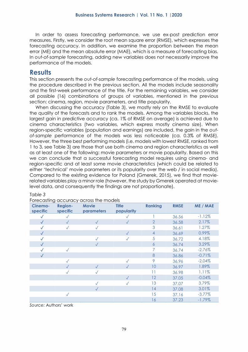
When discussing the accuracy (Table 3), we mostly rely on the RMSE to evaluate

the quality of the forecasts and to rank the models. Among the variables blocks, the

largest gain in predictive accuracy (ca. 1% of RMSE on average) is achieved due to

cinema characteristics (two variables, which express mostly cinema size). When

region-specific variables (population and earnings) are included, the gain in the out-

of-sample performance of the models was less noticeable (ca. 0.3% of RMSE).

However, the three best performing models (i.e. models with lowest RMSE, ranked from

1 to 3, see Table 3) are those that use both cinema and region characteristics as well

as at least one of the following: movie parameters or movie popularity. Based on this

we can conclude that a successful forecasting model requires using cinema- and

region-specific and at least some movie characteristics (which could be related to

either ‘technical’ movie parameters or its popularity over the web / in social media).

Compared to the existing evidence for Poland (Gmerek, 2015), we find that movie-

related variables play a minor role (however, the study by Gmerek operated at movie-

level data, and consequently the findings are not proportionate).

Table 3

Forecasting accuracy across the models Cinema-

specific

Region-

specific

Movie

parameters

Title

popularity

Ranking RMSE ME / MAE

✓ ✓ ✓ 1 36.56 -1.12%

✓ ✓ ✓ ✓ 2 36.58 2.17%

✓ ✓ ✓ 3 36.61 1.27%

✓ ✓ 4 36.69 0.99%

✓ ✓ ✓ 5 36.72 4.18%

✓ ✓ 6 36.74 3.29%

✓ ✓ 7 36.74 -2.76%

✓ 8 36.86 -0.71%

✓ ✓ 9 36.96 -2.04%

✓ ✓ ✓ 10 36.97 1.89%

✓ ✓ 11 36.98 1.11%

✓ 12 37.05 -0.04%

✓ ✓ 13 37.07 3.79%

✓ 14 37.08 3.01%

✓ 15 37.16 -3.77%

16 37.23 -1.79%


80


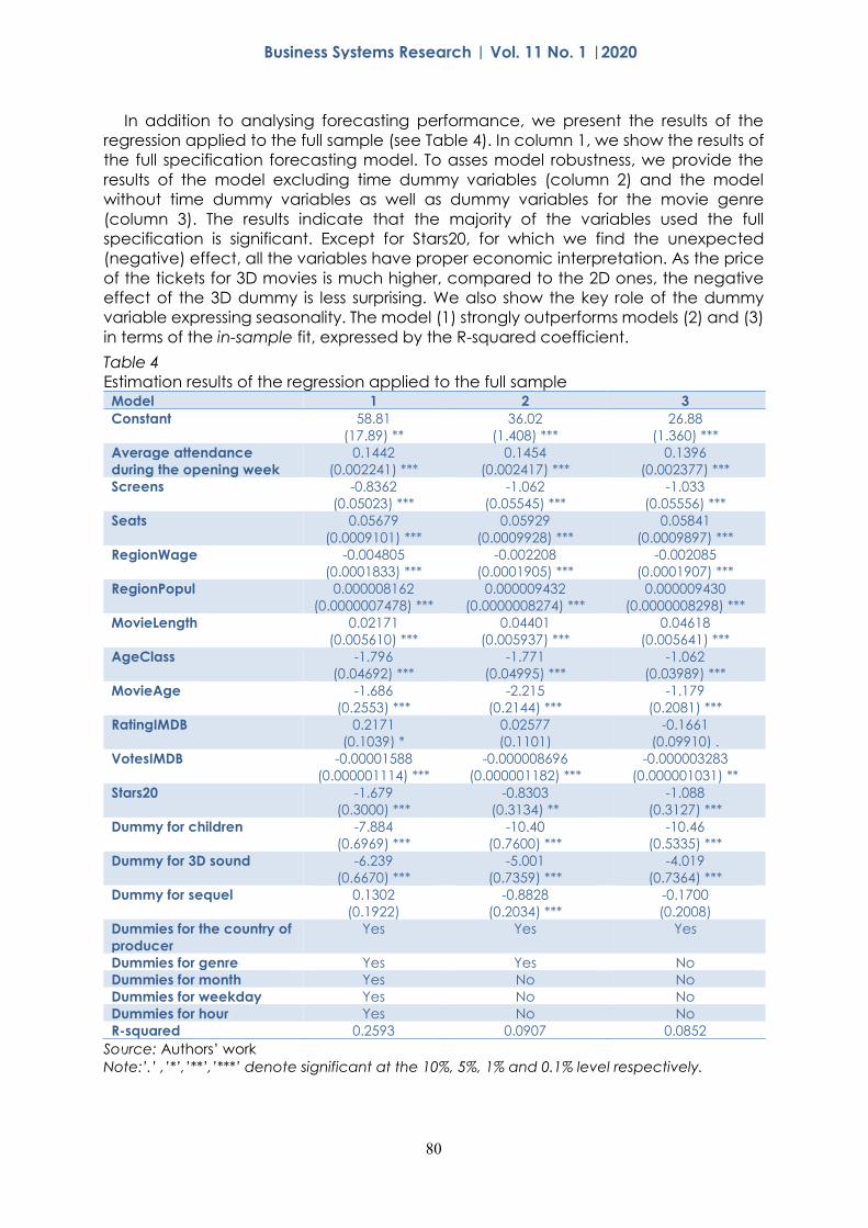
In addition to analysing forecasting performance, we present the results of the

regression applied to the full sample (see Table 4). In column 1, we show the results of

the full specification forecasting model. To asses model robustness, we provide the

results of the model excluding time dummy variables (column 2) and the model

without time dummy variables as well as dummy variables for the movie genre

(column 3). The results indicate that the majority of the variables used the full

specification is significant. Except for Stars20, for which we find the unexpected

(negative) effect, all the variables have proper economic interpretation. As the price

of the tickets for 3D movies is much higher, compared to the 2D ones, the negative

effect of the 3D dummy is less surprising. We also show the key role of the dummy

variable expressing seasonality. The model (1) strongly outperforms models (2) and (3)

in terms of the in-sample fit, expressed by the R-squared coefficient.

Table 4

Estimation results of the regression applied to the full sample Model 1 2 3

Constant 58.81

(17.89) **

36.02

(1.408) ***

26.88

(1.360) ***

Average attendance

during the opening week

0.1442

(0.002241) ***

0.1454

(0.002417) ***

0.1396

(0.002377) ***

Screens -0.8362

(0.05023) ***

-1.062

(0.05545) ***

-1.033

(0.05556) ***

Seats 0.05679

(0.0009101) ***

0.05929

(0.0009928) ***

0.05841

(0.0009897) ***

RegionWage -0.004805

(0.0001833) ***

-0.002208

(0.0001905) ***

-0.002085

(0.0001907) ***

RegionPopul 0.000008162

(0.0000007478) ***

0.000009432

(0.0000008274) ***

0.000009430

(0.0000008298) ***

MovieLength 0.02171

(0.005610) ***

0.04401

(0.005937) ***

0.04618

(0.005641) ***

AgeClass -1.796

(0.04692) ***

-1.771

(0.04995) ***

-1.062

(0.03989) ***

MovieAge -1.686

(0.2553) ***

-2.215

(0.2144) ***

-1.179

(0.2081) ***

RatingIMDB 0.2171

(0.1039) *

0.02577

(0.1101)

-0.1661

(0.09910) .

VotesIMDB -0.00001588

(0.000001114) ***

-0.000008696

(0.000001182) ***

-0.000003283

(0.000001031) **

Stars20 -1.679

(0.3000) ***

-0.8303

(0.3134) **

-1.088

(0.3127) ***

Dummy for children -7.884

(0.6969) ***

-10.40

(0.7600) ***

-10.46

(0.5335) ***

Dummy for 3D sound -6.239

(0.6670) ***

-5.001

(0.7359) ***

-4.019

(0.7364) ***

Dummy for sequel 0.1302

(0.1922)

-0.8828

(0.2034) ***

-0.1700

(0.2008)

Dummies for the country of

producer

Yes Yes Yes

Dummies for genre Yes Yes No

Dummies for month Yes No No

Dummies for weekday Yes No No

Dummies for hour Yes No No

R-squared 0.2593 0.0907 0.0852


Note:’.’ ,’*’,’**’,’***’ denote significant at the 10%, 5%, 1% and 0.1% level respectively.

81


Robustness checks In addition to the results presented in the previous section, we perform several

robustness checks. Below we show the detailed results of the two of the checks.

Firstly, we exclude first-week attendance from the set of variables. This makes it

possible to consider even more parsimonious models. Secondly, we perform a

robustness check related to heteroscedasticity. Heteroscedasticity is typically

encountered in regressions using large microeconomic samples. It was detected in

our models by using Breusch-Pagan tests, at a 1% significance level. In order to tackle

this issue, we apply a two-step weighted least squares regression (henceforth: WLS)

assuming that the variance of errors is proportional to the absolute value of fitted

values from the corresponding OLS model (i.e., similar to the specification of the

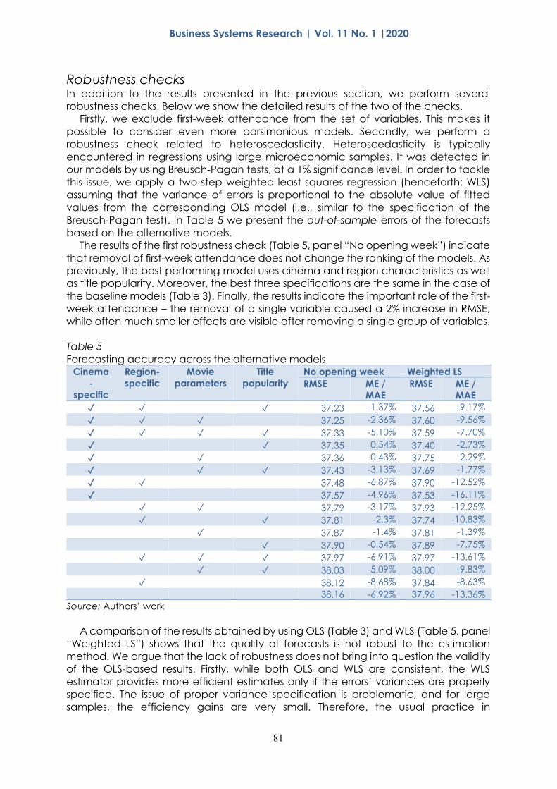
Breusch-Pagan test). In Table 5 we present the out-of-sample errors of the forecasts

based on the alternative models.

The results of the first robustness check (Table 5, panel “No opening week”) indicate

that removal of first-week attendance does not change the ranking of the models. As

previously, the best performing model uses cinema and region characteristics as well

as title popularity. Moreover, the best three specifications are the same in the case of

the baseline models (Table 3). Finally, the results indicate the important role of the first-

week attendance – the removal of a single variable caused a 2% increase in RMSE,

while often much smaller effects are visible after removing a single group of variables.

Table 5

Forecasting accuracy across the alternative models Cinema

-

specific

Region-

specific

Movie

parameters

Title

popularity

No opening week Weighted LS

RMSE ME /

MAE

RMSE ME /

MAE

✓ ✓ ✓ 37.23 -1.37% 37.56 -9.17%

✓ ✓ ✓ 37.25 -2.36% 37.60 -9.56%

✓ ✓ ✓ ✓ 37.33 -5.10% 37.59 -7.70%

✓ ✓ 37.35 0.54% 37.40 -2.73%

✓ ✓ 37.36 -0.43% 37.75 2.29%

✓ ✓ ✓ 37.43 -3.13% 37.69 -1.77%

✓ ✓ 37.48 -6.87% 37.90 -12.52%

✓ 37.57 -4.96% 37.53 -16.11%

✓ ✓ 37.79 -3.17% 37.93 -12.25%

✓ ✓ 37.81 -2.3% 37.74 -10.83%

✓ 37.87 -1.4% 37.81 -1.39%

✓ 37.90 -0.54% 37.89 -7.75%

✓ ✓ ✓ 37.97 -6.91% 37.97 -13.61%

✓ ✓ 38.03 -5.09% 38.00 -9.83%

✓ 38.12 -8.68% 37.84 -8.63%

38.16 -6.92% 37.96 -13.36%


A comparison of the results obtained by using OLS (Table 3) and WLS (Table 5, panel

“Weighted LS”) shows that the quality of forecasts is not robust to the estimation

method. We argue that the lack of robustness does not bring into question the validity

of the OLS-based results. Firstly, while both OLS and WLS are consistent, the WLS

estimator provides more efficient estimates only if the errors’ variances are properly

specified. The issue of proper variance specification is problematic, and for large

samples, the efficiency gains are very small. Therefore, the usual practice in

82


microeconometrics is to use OLS and heteroscedasticity-consistent standard errors of

the estimates (Cameron and Trivedi, 2005, p. 81). Secondly, the accuracy of the WLS-

based forecasts is significantly worse than the accuracy of the OLS-based forecasts.

For the benchmark specification, we get RMSEs equal to 37.23 and 38.16, respectively

for WLS and OLS. Moreover, for the best model, the RMSEs are 36.56 and 37.23,

respectively for WLS and OLS. In addition, most of the WLS forecasts are systematically

biased (i.e., average ME / MAE across the models is 10% in absolute terms; see Table

4). Clearly, OLS-based forecasts outperform those based on WLS. Following the theory

behind WLS estimation, this may indicate the misspecification of the variance of the

error term. Similar results are obtained under several standard assumptions on the

variances of the errors (and consequently the weights applied by WLS). Further

robustness check consisted of the following: (i) including intra-day seasonality

expressed in a 4-hour interval (instead of a 1-hour interval), (ii) including the region’s

unemployment rate (instead of average earnings), (iii) including a dummy variable

representing national holidays in addition to weekly dummies, and (iv) shortening the

out-of-sample period.

The results appear to be robust with respect to these modifications (detailed results

are available upon request). As mentioned, we also consider several variants of non-

linear models (including an exponential specification or adding squares of the

continuous variables). However, including non-linear specifications does not improve

the out-of-sample accuracy compared to the models presented in the previous

section. The inspection of the descriptive statistics suggests that the dataset may suffer

from outliers (which might be due to blockbusters, e.g. De Vany, 2003; Koçaş and

Akkan, 2016). We also checked the models using a regression method robust to outliers

(namely Huber regression) instead of OLS. The results indicate that applying robust

regression to deal with outliers increased the aggregate forecast errors (e.g. RMSE, on

average, by 5%).

Discussion We analysed a number of forecasting models based on data at the movie show level.

Such a dataset has not been analysed in the literature so far. However, we discuss the

results by comparing them with the studies using a large set of variables that overlap

partially with our set of regressors.

Walls (2005) analysed the box-office revenues and identified that a sequel status

improves performance, ceteris paribus while imposing restrictions on the viewer's age

decreases performance. The results presented in Table 4 indicate the equivalent

relationship for similar movie performance indicators (number of tickets sold).

Furthermore, Walls (2005) indicated a positive effect of the movie opening proxied by

the number of screens during the first (opening) week, while our results are analogue,

but based on an aggregate attendance during the opening week.

As in Walls (2005), we found small gains from including movie genres (after including

9 genre dummies increases R-squared only by 0.005, see Table 4). On the other hand,

Treme et al. (2018) and Marshall (2013) got opposite results that were statistically

significant at least for part of genre dummies. In addition, Treme et al. (2018) and

Marshall et al. (2013) identified the negative effects of age classification (age rating)

on the box office performance.

Treme et al. (2018) estimated the determinants of movie attendance. As in our

study, they found positive effects of the number of top stars in the cast. A similar effect

was found by Walls (2005), but he investigated a dummy for the appearance of at

least one star, rather than the number of stars. In our regression, we surprisingly

estimated that effects as negative.

83


Finally, both Treme et al. (2018) and Marshall et al. (2013) confirmed the positive

influence of the reviews on movie attendance. Marshall (2013) included the quality of

the reviews made by professional critics, while Treme et al. (2018) covered both the

reviews by the critics and the viewers. In our study, we included the movie rating

based on the opinions of the IMDb users, which covers non-professional opinions rather

than professional critics.

The results presented in the paper could be also compared to the literature focused

on the Polish cinema industry. To our best knowledge, the only empirical study

examining cinema attendance in Poland was the one by Gmerek (2015). While

Gmerek (2015) operated at movie-level data, we can confront the results with respect

to variables directly related to movie titles (i.e. ‘movie parameters’ and ‘title

popularity’ in our terminology). Our results are mostly consistent with the ones by

Gmerek (2015). More specifically, Gmerek found a positive impact of sequel status,

viewers rating and opening week attendance. In contrast to our findings, Gmerek

(2015) found a significant impact of movie genre, but consider only comedy and

history genres, while we included 10 main categories and estimated small gains from

including genre dummies. A large number of papers, including our study, stressed the

positive effects of number stars in the cast. However, Gmerek did not find this variable

as significant.

Implications for practice From a practical point of view, the models developed in the paper may be directly

applied in the cinema industry. We do not claim that the list of variables used in the

best performing model is valid for all cinema operators. However, our main conclusion

should be universal. Therefore, at least for the cinemas operating in Central and

Eastern Europe one can gain from including a broad set of predictors related to the

movie title, region, and cinema. These models could be used in the cinema operator

system, mainly to assist in planning the cinema programmes. More specifically,

accurate forecasts may increase the volume of ticket sales when there is strong

demand heterogeneity across the movie titles. For instance, when in the given cinema

the model predicts higher attendance for the movie ‘A’ compared to the ‘B’, one

may assign the ‘A’ to the room of higher capacity. Furthermore, the accurate

demand prediction may be used for improving price policy (e.g. to apply for price

discrimination or promotion).

It should also be underlined that typically the scale of business operations of cinema

operators is large. In these circumstances, even small differences of RMSEs across the

models may contribute to substantial differences in revenues.

Contributions to the literature This paper contributes to the literature in at least three ways.

Firstly, most of the studies focus on a single factor or a group of factors (most often

movie characteristics) that may influence cinema attendance or revenues (e.g.,

Walls, 2005; Marshall et al., 2013; Treme et al., 2018). As Litman (1983), Hofmann-Stölting

et al. (2017) and Wu et al. (2018) showed, it pays off to include various factors when

forecasting the success of movies. To our best knowledge, our set of variables,

including factors related to cinema and movie characteristics, title popularity and the

economic conditions of the region, is more comprehensive than those used in the

literature so far.

Secondly, the vast majority of papers analyse the data at the movie-level (e.g.,

Hand, 2002; Marshall et al., 2013; Gmerek, 2015; Treme et al., 2018). Another notable

strand of literature explores the propensity of the individual or household to participate

84


in cultural events such as movie-going. These studies are mostly interested in how

socioeconomic factors influence individuals’ attendance at the cinema. Our paper is

closer to the first strand, however, we explore cinema attendance on the individual

show level, which allows including also characteristics of the cinema or specific

cinema room as well as intra-day and weekly seasonality.

Thirdly, previous empirical studies aimed at estimating the determinants of

attendance. This allows identifying the size and statistical significance of each

variable. In this paper, we go beyond this approach and focus on out-of-sample

predictive performance with respect to the variable selection. This means we are

interested in finding the variables useful in one week ahead prediction, rather than

the ones with high in-sample contemporary correlation.

Conclusion In this paper, we investigated cinema attendance forecasting based on data from a

large Polish cinema operator. Our models explain the attendance of individual movie

shows. The research strategy was to use several groups of variables in an out-of-

sample forecasting procedure. In addition to movie parameters that are routinely

used in the literature, we include cinema-specific, region-specific and movie

popularity data. From a statistical point of view, using a large set of variables eliminates

(or significantly reduces) omitted variable bias. The models developed in the paper

operate on highly disaggregated data (i.e., at the individual show level) and similarly

to machine-learning models, they may assist in making the business decision (Bose

and Mahapatra, 2001). Our results can be used in planning the repertoire and

allocating movies to the cinema rooms, contributing to the increase in the number of

tickets sold. Our results may also be useful for other enterprises from the entertainment

industry where cultural events are planned.

Our main conclusion is that forecasting the attendance of individual movie shows

is feasible, contrary to the suggestions contained in some earlier studies. It turns out

that the best performing models, in terms of aggregate accuracy, are those that

include a wide set of variables, i.e., cinema- and region-specific variables in addition

to movie parameters (such as genre, running time, age classification, etc.) or title

popularity (number of votes and average rating from IMDb). The results are robust with

respect to expressing seasonality, modifying regional characteristics or shortening the

out-of-sample period.

Limitations and further research The first limitation of the research is the fact that we use the dataset from a single Polish

cinema operator. The question emerges if the results are also valid for other countries.

We believe that to some extent we can extrapolate the results to other Central and

Eastern European countries. The evidence from the literature suggests substantial

cross-country similarities regarding the cinema industry. For example, Central and

Eastern European countries have comparable movie preferences (Fu and

Govindaraju, 2010) and the income elasticity of cinema demand is similar to the

United States (Luňáček and Feldbabel, 2014). The second concern is the dataset

representativeness – one may doubt if the database derived from one company

describe the entire industry. Unfortunately, based on the data collected for this study

we are not able to fully address this issue.

In our study, we make use of the data from social media. These data, however, are

limited to average rating and the number of votes collected from IMDb. Employing

additional sources of social media data, including Facebook or Twitter data, is a

85


natural candidate for further research. Within these data, one can pick both numbers

of ‘likes’, ‘favorites’, ‘followers’ as well as the tone of word-of-mouth reviews.

Clearly, cinema attendance could be also related to weather conditions. Similarly,

the negative effects of rain or snow have been recently found for museum

attendance (Cuffe, 2018). However, given the very low quality of weather forecasts

with a horizon longer than three days, a direct application for forecasting at one week

ahead horizon is problematic.

Finally, most of the predictors used in the study are categorical or vary only across

the regions. This could be the possible reason for the similar or even better

performance of linear models when compared to the non-linear alternatives.

Subsequently, in future research, we can also consider applying machine learning

models such as support vector machines or neural networks.

References 1. Ainslie, A., Drèze, X., Zufryden, F. (2005),” Modeling movie life cycles and market share“,

Marketing Science, Vol. 24, No. 3, pp. 508-517.

2. Baranowski, P., Komor, M., Wójcik, S. (2018),” Whose feedback matters? Empirical

evidence from online auctions “, Applied Economics Letters, Vol. 25, No. 17, pp. 1226–1229.

3. Bloom, N. (2014),” Fluctuations in uncertainty”, Journal of Economic Perspectives, Vol. 28,

No. 2, pp. 153-76.

4. Bose, I., Mahapatra, R.K. (2001),” Business data mining—A machine learning perspective

“, Information & Management, Vol. 39, No. 3, pp. 211–225.

5. Bukovina, J. (2016), “Social media big data and capital markets—An overview”, Journal

of Behavioral and Experimental Finance, Vol. 11, pp. 18-26.

6. Cameron, S. (1988),” The Impact of Video Recorders on Cinema Attendance“, Journal of

Cultural Economics, Vol. 12, No. 1, pp. 73–80.

7. Cameron, S. (1999),” Rational addiction and the demand for cinema“, Applied Economics

Letters, Vol. 6, No. 9, pp. 617-620.

8. Cameron, A.C., Trivedi, P.K. (2005),” Microeconometrics: Methods and applications “,

Cambridge University Press.

9. Casson, M. (2006),” Culture and economic performance“, in Ginsburg, V.A., Throsby, D.

(Eds.), Handbook of the Economics of Art and Culture, 1, pp. 359–397.

10. Collins A., Hand, C. (2005),” Analyzing Moviegoing Demand: An Individual-level Cross-

sectional Approach“, Managerial and Decision Economics, Vol. 26, No. 5, pp. 319–330.

11. Collins, A., Scorcu, A.E., Zanola, R. (2009),” Distribution Conventionality in the Movie Sector:

An Econometric Analysis of Cinema Supply“, Managerial and Decision Economics, Vol. 30,

No. 8, pp. 517–527.

12. Craig, C. S., Greene, W. H., Versaci, A. (2015), “E-word of mouth: Early predictor of

audience engagement: How pre-release “e-WOM” drives box-office outcomes of

movies“, Journal of Advertising Research, Vol. 55, No. 1, pp. 62-72.

13. Cuffe, H.E. (2018),” Rain and museum attendance: Are daily data fine enough?“, Journal

of Cultural Economics, Vol. 42, No. 2, pp. 213–241.

14. De Vany, A. (2003),” Hollywood economics: How extreme uncertainty shapes the film

industry“, Routledge.

15. De Vany, A.S., Walls, W.D. (1999),” Uncertainty in the Movie Industry: Does Star Power

Reduce the Terror of the Box Office? “, Journal of Cultural Economics, Vol. 23, No. 4, pp.

285–318.

16. Dellarocas, C., Zhang, X., Awad, N.F. (2007),” Exploring the value of online product reviews

in forecasting sales: The case of motion pictures “, Journal of Interactive Marketing, Vol.

21, No. 4, pp. 23–45.

17. Dewenter, R., Westermann, M. (2005),” Cinema demand in Germany “, Journal of Cultural

Economics, Vol. 29, No. 3, pp. 213–231.

18. Ding, C., Cheng, H. K., Duan, Y., Jin, Y. (2017),” The power of the “like” button: The impact

of social media on box office “, Decision Support Systems, Vol. 94, pp. 77-84.

86


19. Doury, N. (2001),” Successfully integrating cinemas into retail and leisure complexes: An

operator's perspective “, Journal of Retail & Leisure Property, Vol. 1, No. 2, pp. 119–126.

20. Duan, W., Gu, B., Whinston, A.B. (2008),” Do online reviews matter? — An empirical

investigation of panel data “, Decision Support Systems, Vol. 45, No. 4, pp. 1007–1016.

21. Feng, G. C. (2017), ”The dynamics of the Chinese film industry: factors affecting Chinese

audiences’ intentions to see movies“, Asia Pacific Business Review, Vol. 23, No. 5, pp. 658-

676.

22. Fu, W.W., Govindaraju, A. (2010), ”Explaining global box-office tastes in Hollywood films:

Homogenization of national audiences’ movie selections“, Communication Research, Vol.

37, No. 2, pp. 215–238.

23. Goczek, Ł., Witkowski, B. (2016), “Determinants of card payments”, Applied Economics,

Vol. 48, No. 16, pp. 1530-1543.

24. Gmerek, N. (2015), ”The determinants of Polish movies’ box office performance in Poland“,

Journal of Marketing and Consumer Behaviour in Emerging Markets, Vol. 1, No. 1, pp. 15–

35.

25. Hand, C. (2002), ”The Distribution and Predictability of Cinema Admissions“, Journal of

Cultural Economics, Vol. 26, No. 1, pp. 53–64.

26. Hand, C., Judge, G. (2012), ”Searching for the picture: Forecasting UK cinema admissions

using Google Trends data“, Applied Economics Letters, Vol. 19, No. 11, pp. 1051–1055.

27. Hofmann-Stölting, C., Clement, M., Wu, S., Albers, S. (2017), “Sales forecasting of new

entertainment media products”, Journal of Media Economics, Vol. 30, No. 3, pp. 143-171.

28. Jansen, C. (2005), ”The performance of German motion pictures, profits and subsidies:

Some empirical evidence“, Journal of Cultural Economics, Vol. 29, No. 3, pp. 191-212.

29. Jeffrey, D., Barden, R. R. (2001), ”Multivariate models of hotel occupancy performance

and their implications for hotel marketing”, International Journal of Tourism Research, Vol.

3, No. 1, pp. 33-44.

30. Jones, S.G. (1986),” Trends in the Leisure Industry since the Second World War “, The Service

Industries Journal, Vol. 6, No. 3, pp. 330-348.

31. Koçaş, C., Akkan, C. (2016), “A system for pricing the sales distribution from blockbusters to

the long tail“, Decision Support Systems, Vol. 89, pp. 56-65.

32. Klinger, T., Lanzendorf, M. (2016), “Moving between mobility cultures: what affects the

travel behavior of new residents?”, Transportation, Vol. 43, No. 2, pp. 243-271.

33. Li, J. (2012), ”From “D-Buffs” to the “D-Generation”: Piracy, Cinema, and An Alternative

Public Sphere in Urban China“, International Journal of Communication, Vol. 6, pp. 542–

563.

34. Litman, B.R. (1983), ”Predicting the Success of Theatrical Movies: An Empirical Study“,

Journal of Popular Culture, Vol. 16, pp. 159–175.

35. Luňáček, J., Feldbabel, V. (2014), ”Elasticity of demand of the Czech consumer“, Acta

Universitatis Agriculturae et Silviculturae Mendelianae Brunensis, Vol. 59, No. 7, pp. 225–

236.

36. Machowska, D. (2018), ”Investigating the role of customer churn in the optimal allocation

of offensive and defensive advertising: The case of the competitive growing market“,

Economics and Business Review, Vol. 4, No. 2, pp. 3–23.

37. MacMillan, P., Smith, I. (2001), ”Explaining post-war cinema attendance in Great Britain“,

Journal of Cultural Economics, Vol. 25, No. 2, pp. 91-108.

38. Makridakis, S., Hogarth, R. M., Gaba, A. (2009), “Forecasting and uncertainty in the

economic and business world“, International Journal of Forecasting, Vol. 25, No. 4, pp. 794-

812.

39. Marshall, P., Dockendorff, M., Ibáñez, S. (2013), “A forecasting system for movie

attendance“, Journal of Business Research, Vol. 66, pp. 1800–1806.

40. Moore, A. (2017), “Measuring economic uncertainty and its effects“, Economic Record,

Vol. 93, No. 303, pp. 550-575.

41. Nelson, R. A., Donihue, M. R., Waldman, D. M., Wheaton C. (2001), ”What’s an Oscar

worth?“, Economic Inquiry, Vol. 39, No. 1, pp. 1-16.

42. Pautz, M. C. (2002), ”The decline in average weekly cinema attendance, 1930-2000“,

Issues in political economy, Vol. 11, pp. 1-19.

87


43. Sharda, R., Delen, D. (2006), ”Predicting box-office success of motion pictures with neural

networks“, Expert Systems with Applications, Vol. 30, No. 2, pp. 243–254.

44. Sisto, A., Zanola, R. (2007), ”Cinema and TV: An Empirical Investigation of Italian

Consumers“, In Bianchi, M. (Ed.), The Evolution of Consumption: Theories and Practices

(Advances in Austrian Economics, Volume 10), Emerald Group Publishing Limited, pp.139

– 154.

45. Sztaudynger, M. (2018), ”Macroeconomic Factors and Consumer Loan Repayment”,

Gospodarka Narodowa, Vol. 296, No. 4, pp. 155-177.

46. Treme, J., VanDerPloeg, Z. (2014), ”The twitter effect: Social media usage as a contributor

to movie success”, Economics Bulletin, Vol. 34, No. 2, pp. 793-809.

47. Treme, J., Craig, L.A., Copland, A. (2018), ”Gender and box office performance“, Applied

Economics Letters, Vol. 34, No. 4, pp. 1–5.

48. Walls, W.D. (2005), ”Modeling Movie Success when ‘Nobody Knows Anything’: Conditional

Stable-Distribution Analysis of Film Returns“, Journal of Cultural Economics, Vol. 29, pp. 177–

190.

49. Wayne, M.L. (2018), ”Netflix, Amazon, and branded television content in subscription video

on-demand portals“, Media, Culture & Society, Vol. 40, No. 5, pp. 725-741.

50. Weziak-Bialowolska, D., Białowolski, P., Sacco, P. (2018), ”Involvement With the Arts and

Participation in Cultural Events-Does Personality Moderate Impact on Well-Being?

Evidence from the U.K. Household Panel Survey“, Psychology of Aesthetics, Creativity, and

the Arts, Vol. 13, No. 3, pp. 348-358.

51. Wu, Y., Huang, W., Lu, Y., Liu, J. (2018), “Box office forecasting for a cinema with movie and

cinema attributes”, in IEEE 3rd International Conference on Cloud Computing and Big

Data Analysis (ICCCBDA), IEEE, pp. 385-389.

52. Yang, Z., Cai, J. (2016), “Do regional factors matter? Determinants of hotel industry

performance in China“, Tourism Management, Vol. 52, pp. 242-253.

53. Yu, X., Liu, Y., Huang, X., An, A. (2012), ”Mining online reviews for predicting sales

performance: A case study in the movie domain“, IEEE Transactions on Knowledge and

Data engineering, Vol. 24, No. 4, pp. 720-734.

54. Yuan, H., Xu, W., Li, Q., Lau, R. (2018). “Topic sentiment mining for sales performance

prediction in e-commerce”, Annals of Operations Research, Vol. 270, Issue 1-2, pp. 553-

576.

88


About the authors Paweł Baranowski, Ph.D. is an Associate Professor at the Faculty of Economics and

Sociology, University of Łódź, Institute of Econometrics, Department of Econometrics.

His research interests include applied econometrics, monetary economics as well as

machine learning and natural language processing. He also worked in the National

Bank of Poland (2009-2017) and Commerzbank A.G. (2017-2018). The author can be

contacted at [email protected]

Karol Korczak, Ph.D. is an Assistant Professor at the Faculty of Economics and

Sociology, University of Łódź, Institute of Applied Economics and Informatics,

Department of Computer Science in Economics. His research interests include

applications of IT in business, algorithms and health economics. He has also practical

experience in designing and implementing IT solutions for business. The author can be

contacted at [email protected]

Jarosław Zając, Ph.D. is a Senior Lecturer at the Faculty of Economics and Sociology,

University of Łódź, Institute of Applied Economics and Informatics, Department of

Computer Science in Economics. He has strong business experience, including

business analytics and IT project management, especially for the financial sector. The

author can be contacted at [email protected]

Documents

Forecasting Cinema Attendance at the Movie Show Level