Embed Size (px)
Citation preview
Air Force Institute of Technology Air Force Institute of Technology
AFIT Scholar AFIT Scholar
Theses and Dissertations Student Graduate Works
3-26-2020
Forecasting Attrition by AFSC for the United States Air Force Forecasting Attrition by AFSC for the United States Air Force
Trey S. Pujats
Follow this and additional works at: https://scholar.afit.edu/etd
Part of the Human Resources Management Commons, and the Labor Economics Commons
Recommended Citation Recommended Citation Pujats, Trey S., "Forecasting Attrition by AFSC for the United States Air Force" (2020). Theses and Dissertations. 3200. https://scholar.afit.edu/etd/3200
This Thesis is brought to you for free and open access by the Student Graduate Works at AFIT Scholar. It has been accepted for inclusion in Theses and Dissertations by an authorized administrator of AFIT Scholar. For more information, please contact [email protected].
Forecasting Attrition by AFSCfor the
United States Air Force
THESIS
Trey S Pujats, 2nd Lieutenant, USAF
AFIT-ENS-MS-20-M-166
DEPARTMENT OF THE AIR FORCEAIR UNIVERSITY
AIR FORCE INSTITUTE OF TECHNOLOGY
Wright-Patterson Air Force Base, Ohio
DISTRIBUTION STATEMENT AAPPROVED FOR PUBLIC RELEASE; DISTRIBUTION UNLIMITED.

The views expressed in this document are those of the author and do not reflect theofficial policy or position of the United States Air Force, the United States Army,the United States Department of Defense or the United States Government. Thismaterial is declared a work of the U.S. Government and is not subject to copyrightprotection in the United States.
AFIT-ENS-MS-20-M-166
FORECASTING ATTRITION BY AFSC
FOR THE
UNITED STATES AIR FORCE
THESIS
Presented to the Faculty
Department of Operational Sciences
Graduate School of Engineering and Management
Air Force Institute of Technology
Air University
Air Education and Training Command
in Partial Fulfillment of the Requirements for the
Degree of Master of Science in Operations Research
Trey S Pujats, B.S.
2nd Lieutenant, USAF
March 26, 2020
DISTRIBUTION STATEMENT AAPPROVED FOR PUBLIC RELEASE; DISTRIBUTION UNLIMITED.
AFIT-ENS-MS-20-M-166
FORECASTING ATTRITION BY AFSC
FOR THE
UNITED STATES AIR FORCE
THESIS
Trey S Pujats, B.S.2nd Lieutenant, USAF
Committee Membership:
Dr. Raymond R Hill, Ph.D.Chair
Lt Col Bruce Cox, PH.D.Member
AFIT-ENS-MS-20-M-166
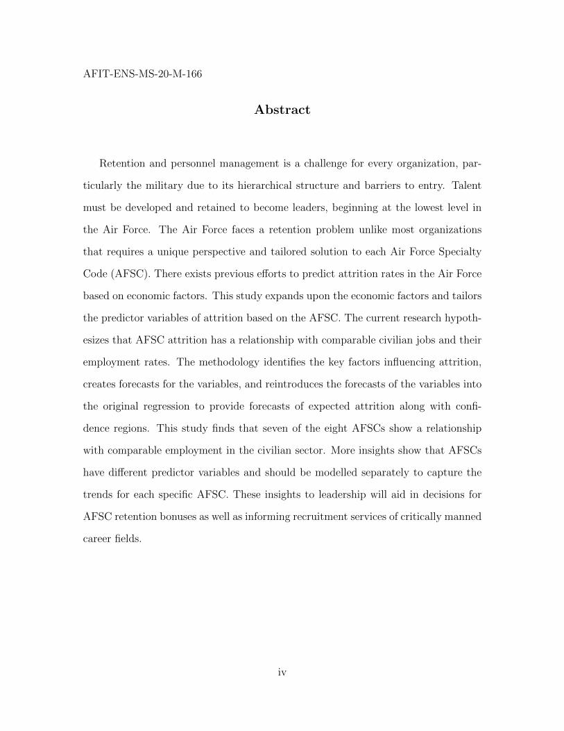
Abstract
Retention and personnel management is a challenge for every organization, par-
ticularly the military due to its hierarchical structure and barriers to entry. Talent
must be developed and retained to become leaders, beginning at the lowest level in
the Air Force. The Air Force faces a retention problem unlike most organizations
that requires a unique perspective and tailored solution to each Air Force Specialty
Code (AFSC). There exists previous efforts to predict attrition rates in the Air Force
based on economic factors. This study expands upon the economic factors and tailors
the predictor variables of attrition based on the AFSC. The current research hypoth-
esizes that AFSC attrition has a relationship with comparable civilian jobs and their
employment rates. The methodology identifies the key factors influencing attrition,
creates forecasts for the variables, and reintroduces the forecasts of the variables into
the original regression to provide forecasts of expected attrition along with confi-
dence regions. This study finds that seven of the eight AFSCs show a relationship
with comparable employment in the civilian sector. More insights show that AFSCs
have different predictor variables and should be modelled separately to capture the
trends for each specific AFSC. These insights to leadership will aid in decisions for
AFSC retention bonuses as well as informing recruitment services of critically manned
career fields.
iv

AFIT-ENS-MS-20-M-166
To my family and friends that have supported me throughout this entire process.
Especially my parents and grandparents who have encouraged me every step of the
way.
v

Acknowledgements
I would like to express my gratitude to my faculty research advisor, Raymond
Hill, Ph.D., for all of his guidance, patience and assistance.
I would like to thank all of my peers and friends that have assisted me through
the coursework and analysis needed for this analysis.
Trey S Pujats
vi
Table of Contents
Page
Abstract . . . . . . . . . . . . . . . . . . . . . . . . . . . . . . . . . . . . . . . . . . . . . . . . . . . . . . . . . . . . . . . iv
Acknowledgements . . . . . . . . . . . . . . . . . . . . . . . . . . . . . . . . . . . . . . . . . . . . . . . . . . . . . . vi
List of Figures . . . . . . . . . . . . . . . . . . . . . . . . . . . . . . . . . . . . . . . . . . . . . . . . . . . . . . . . . . ix
List of Tables . . . . . . . . . . . . . . . . . . . . . . . . . . . . . . . . . . . . . . . . . . . . . . . . . . . . . . . . . . xii
I. Introduction . . . . . . . . . . . . . . . . . . . . . . . . . . . . . . . . . . . . . . . . . . . . . . . . . . . . . . . . 1
1.1 Background . . . . . . . . . . . . . . . . . . . . . . . . . . . . . . . . . . . . . . . . . . . . . . . . . . . . 11.2 Overview . . . . . . . . . . . . . . . . . . . . . . . . . . . . . . . . . . . . . . . . . . . . . . . . . . . . . . . 31.3 Problem Statement . . . . . . . . . . . . . . . . . . . . . . . . . . . . . . . . . . . . . . . . . . . . . . 41.4 Thesis Outline . . . . . . . . . . . . . . . . . . . . . . . . . . . . . . . . . . . . . . . . . . . . . . . . . . 4
II. Literature Review . . . . . . . . . . . . . . . . . . . . . . . . . . . . . . . . . . . . . . . . . . . . . . . . . . . 6
2.1 Overview . . . . . . . . . . . . . . . . . . . . . . . . . . . . . . . . . . . . . . . . . . . . . . . . . . . . . . . 62.2 Military Retention Problem . . . . . . . . . . . . . . . . . . . . . . . . . . . . . . . . . . . . . . . 62.3 Previous Efforts . . . . . . . . . . . . . . . . . . . . . . . . . . . . . . . . . . . . . . . . . . . . . . . . . 72.4 Analytical Techniques . . . . . . . . . . . . . . . . . . . . . . . . . . . . . . . . . . . . . . . . . . . . 9
III. Methodology . . . . . . . . . . . . . . . . . . . . . . . . . . . . . . . . . . . . . . . . . . . . . . . . . . . . . . 11
3.1 Overview . . . . . . . . . . . . . . . . . . . . . . . . . . . . . . . . . . . . . . . . . . . . . . . . . . . . . . 113.2 Data Description . . . . . . . . . . . . . . . . . . . . . . . . . . . . . . . . . . . . . . . . . . . . . . . 113.3 Data Preparation . . . . . . . . . . . . . . . . . . . . . . . . . . . . . . . . . . . . . . . . . . . . . . . 133.4 Regression Analysis . . . . . . . . . . . . . . . . . . . . . . . . . . . . . . . . . . . . . . . . . . . . . 153.5 Box-Jenkins Models . . . . . . . . . . . . . . . . . . . . . . . . . . . . . . . . . . . . . . . . . . . . 183.6 Forecasting Attrition . . . . . . . . . . . . . . . . . . . . . . . . . . . . . . . . . . . . . . . . . . . . 21
IV. Analysis . . . . . . . . . . . . . . . . . . . . . . . . . . . . . . . . . . . . . . . . . . . . . . . . . . . . . . . . . . 23
4.1 Introduction . . . . . . . . . . . . . . . . . . . . . . . . . . . . . . . . . . . . . . . . . . . . . . . . . . . 234.2 11X - Pilot Career Field Analysis . . . . . . . . . . . . . . . . . . . . . . . . . . . . . . . . . 24
4.2.1 Regression Analysis of Pilot Career Field . . . . . . . . . . . . . . . . . . . . 244.2.2 Forecasting Independent Variables . . . . . . . . . . . . . . . . . . . . . . . . . . 254.2.3 Forecasting Attrition . . . . . . . . . . . . . . . . . . . . . . . . . . . . . . . . . . . . . . 26
4.3 17D - Cyber Career Field Analysis . . . . . . . . . . . . . . . . . . . . . . . . . . . . . . . . 274.3.1 Regression Analysis of Cyber Career Field . . . . . . . . . . . . . . . . . . . 274.3.2 Forecasting Independent Variables . . . . . . . . . . . . . . . . . . . . . . . . . . 294.3.3 Forecasting Attrition . . . . . . . . . . . . . . . . . . . . . . . . . . . . . . . . . . . . . . 30
4.4 31P - Security Forces Career Field Analysis . . . . . . . . . . . . . . . . . . . . . . . . 31
vii
Page
4.4.1 Regression Analysis of Security Forces . . . . . . . . . . . . . . . . . . . . . . . 314.4.2 Forecasting Independent Variables . . . . . . . . . . . . . . . . . . . . . . . . . . 324.4.3 Forecasting Attrition . . . . . . . . . . . . . . . . . . . . . . . . . . . . . . . . . . . . . . 33
4.5 32E - Civil Engineering Career Field Anaysis . . . . . . . . . . . . . . . . . . . . . . . 344.5.1 Regression Analysis of Civil Engineering . . . . . . . . . . . . . . . . . . . . . 344.5.2 Forecasting Independent Variables . . . . . . . . . . . . . . . . . . . . . . . . . . 364.5.3 Forecasting Attrition . . . . . . . . . . . . . . . . . . . . . . . . . . . . . . . . . . . . . . 37
4.6 61A - Operations Research Analyst Career Field Analysis . . . . . . . . . . . . 384.6.1 Regression Analysis of Operations Research . . . . . . . . . . . . . . . . . . 384.6.2 Forecasting Independent Variables . . . . . . . . . . . . . . . . . . . . . . . . . . 404.6.3 Forecasting Attrition . . . . . . . . . . . . . . . . . . . . . . . . . . . . . . . . . . . . . . 41
4.7 62E - Engineering Career Field Analysis . . . . . . . . . . . . . . . . . . . . . . . . . . . 424.7.1 Regression Analysis of Engineering . . . . . . . . . . . . . . . . . . . . . . . . . . 424.7.2 Forecasting Independent Variables . . . . . . . . . . . . . . . . . . . . . . . . . . 444.7.3 Forecasting Attrition . . . . . . . . . . . . . . . . . . . . . . . . . . . . . . . . . . . . . . 45
4.8 63A - Acquisitions Career Field Analysis . . . . . . . . . . . . . . . . . . . . . . . . . . 464.8.1 Regression Analysis of Acquisitions . . . . . . . . . . . . . . . . . . . . . . . . . 464.8.2 Forecasting Independent Variables . . . . . . . . . . . . . . . . . . . . . . . . . . 474.8.3 Forecasting Attrition . . . . . . . . . . . . . . . . . . . . . . . . . . . . . . . . . . . . . . 48
4.9 64P - Contracting Career Field Analysis . . . . . . . . . . . . . . . . . . . . . . . . . . . 494.9.1 Regression Analysis of Contracting . . . . . . . . . . . . . . . . . . . . . . . . . 494.9.2 Forecasting Independent Variables . . . . . . . . . . . . . . . . . . . . . . . . . . 504.9.3 Forecasting Attrition . . . . . . . . . . . . . . . . . . . . . . . . . . . . . . . . . . . . . . 52
4.10 Concluding Remarks . . . . . . . . . . . . . . . . . . . . . . . . . . . . . . . . . . . . . . . . . . . . 53
V. Conclusions and Future Research . . . . . . . . . . . . . . . . . . . . . . . . . . . . . . . . . . . . . 54
5.1 Review . . . . . . . . . . . . . . . . . . . . . . . . . . . . . . . . . . . . . . . . . . . . . . . . . . . . . . . . 545.2 Results . . . . . . . . . . . . . . . . . . . . . . . . . . . . . . . . . . . . . . . . . . . . . . . . . . . . . . . 545.3 Recommendations . . . . . . . . . . . . . . . . . . . . . . . . . . . . . . . . . . . . . . . . . . . . . . 555.4 Future Research . . . . . . . . . . . . . . . . . . . . . . . . . . . . . . . . . . . . . . . . . . . . . . . . 56
Appendix A: Pilot Model Adequacy . . . . . . . . . . . . . . . . . . . . . . . . . . . . . . . . . . . . . . . 59Appendix B: Cyber Model Adequacy . . . . . . . . . . . . . . . . . . . . . . . . . . . . . . . . . . . . . . 61Appendix C: Security Forces Model Adequacy . . . . . . . . . . . . . . . . . . . . . . . . . . . . . . 63Appendix D: Civil Engineer Model Adequacy . . . . . . . . . . . . . . . . . . . . . . . . . . . . . . . 65Appendix E: Analyst Model Adequacy . . . . . . . . . . . . . . . . . . . . . . . . . . . . . . . . . . . . . 67Appendix F: Engineer Model Adequacy . . . . . . . . . . . . . . . . . . . . . . . . . . . . . . . . . . . . 69Appendix G: Acquisitions Engineer Model Adequacy . . . . . . . . . . . . . . . . . . . . . . . . . 71Appendix H: Contracting Model Adequacy . . . . . . . . . . . . . . . . . . . . . . . . . . . . . . . . . 73Appendix I: Example R Code for Pilot AFSC . . . . . . . . . . . . . . . . . . . . . . . . . . . . . . . 83Bibliography . . . . . . . . . . . . . . . . . . . . . . . . . . . . . . . . . . . . . . . . . . . . . . . . . . . . . . . . . . . 84
viii
List of Figures
Figure Page
1 Regression on Pilot Attrition . . . . . . . . . . . . . . . . . . . . . . . . . . . . . . . . . . . . . 25
2 Time Series Forecast on Pilot Independent Variables:The light blue region shows 95% confidence region andthe dark blue region shows 80% confidence region. . . . . . . . . . . . . . . . . . . 26
3 Forecast of Pilot Attrition . . . . . . . . . . . . . . . . . . . . . . . . . . . . . . . . . . . . . . . 27
4 Regression on Cyber Attrition . . . . . . . . . . . . . . . . . . . . . . . . . . . . . . . . . . . . 28
5 Time Series Forecast on Cyber Independent Variables:The light blue region shows 95% confidence region andthe dark blue region shows 80% confidence region. . . . . . . . . . . . . . . . . . . 29
6 Forecast of Cyber Attrition . . . . . . . . . . . . . . . . . . . . . . . . . . . . . . . . . . . . . . 30
7 Security Forces Regression . . . . . . . . . . . . . . . . . . . . . . . . . . . . . . . . . . . . . . . 32
8 Time Series Forecast on Security Forces IndependentVariables: The light blue region shows 95% confidenceregion and the dark blue region shows 80% confidenceregion. . . . . . . . . . . . . . . . . . . . . . . . . . . . . . . . . . . . . . . . . . . . . . . . . . . . . . . . . 33
9 Forecast of Security Forces Attrition . . . . . . . . . . . . . . . . . . . . . . . . . . . . . . 34
10 Civil Engineer Regression on Attrition . . . . . . . . . . . . . . . . . . . . . . . . . . . . . 36
11 Time Series Forecast on Civil Engineer IndependentVariables: The light blue region shows 95% confidenceregion and the dark blue region shows 80% confidenceregion. . . . . . . . . . . . . . . . . . . . . . . . . . . . . . . . . . . . . . . . . . . . . . . . . . . . . . . . . 37
12 Forecast of Civil Engineer Attrition . . . . . . . . . . . . . . . . . . . . . . . . . . . . . . . 38
13 Operations Research Regression on Attrition . . . . . . . . . . . . . . . . . . . . . . . 40
14 Time Series Forecast on Analyst Independent Variables:The light blue region shows 95% confidence region andthe dark blue region shows 80% confidence region. . . . . . . . . . . . . . . . . . . 41
15 Forecast of Analyst Attrition . . . . . . . . . . . . . . . . . . . . . . . . . . . . . . . . . . . . . 42
16 Engineers Regression on Attrition . . . . . . . . . . . . . . . . . . . . . . . . . . . . . . . . . 43
ix
Figure Page
17 Time Series Forecast on Engineering IndependentVariables: The light blue region shows 95% confidenceregion and the dark blue region shows 80% confidenceregion. . . . . . . . . . . . . . . . . . . . . . . . . . . . . . . . . . . . . . . . . . . . . . . . . . . . . . . . . 44
18 Forecast of Engineer Attrition . . . . . . . . . . . . . . . . . . . . . . . . . . . . . . . . . . . . 45
19 Acquisitions Regression on Attrition . . . . . . . . . . . . . . . . . . . . . . . . . . . . . . . 47
20 Time Series Forecast on Acquisitions IndependentVariables: The light blue region shows 95% confidenceregion and the dark blue region shows 80% confidenceregion. . . . . . . . . . . . . . . . . . . . . . . . . . . . . . . . . . . . . . . . . . . . . . . . . . . . . . . . . 47
21 Forecast of Acquisitions Attrition . . . . . . . . . . . . . . . . . . . . . . . . . . . . . . . . . 49
22 Regression on Contracting Attrition . . . . . . . . . . . . . . . . . . . . . . . . . . . . . . . 50
23 Time Series Forecast on Contracting IndependentVariables: The light blue region shows 95% confidenceregion and the dark blue region shows 80% confidenceregion. . . . . . . . . . . . . . . . . . . . . . . . . . . . . . . . . . . . . . . . . . . . . . . . . . . . . . . . . 52
24 Forecasts of Contracting Attrition . . . . . . . . . . . . . . . . . . . . . . . . . . . . . . . . . 53
25 Pilot Regression Residual Analysis . . . . . . . . . . . . . . . . . . . . . . . . . . . . . . . . 58
26 Pilot Variable ARIMA Residual Analysis . . . . . . . . . . . . . . . . . . . . . . . . . . 58
27 Pilot Forecast Model Validation . . . . . . . . . . . . . . . . . . . . . . . . . . . . . . . . . . 59
28 Cyber Regression Residual Analysis . . . . . . . . . . . . . . . . . . . . . . . . . . . . . . . 60
29 Cyber Variable ARIMA Residual Analysis . . . . . . . . . . . . . . . . . . . . . . . . . 60
30 Cyber Forecast Model Validation . . . . . . . . . . . . . . . . . . . . . . . . . . . . . . . . . 61
31 Security Forces Regression Residual Analysis . . . . . . . . . . . . . . . . . . . . . . . 62
32 Security Forces Variable ARIMA Residual Analysis . . . . . . . . . . . . . . . . . 62
33 Security Forces Forecast Model Validation . . . . . . . . . . . . . . . . . . . . . . . . . 63
34 Civil Engineer Regression Residual Analysis . . . . . . . . . . . . . . . . . . . . . . . . 64
35 Civil Engineer Variable ARIMA Residual Analysis . . . . . . . . . . . . . . . . . . 64
x
Figure Page
36 Civil Engineer Forecast Model Validation . . . . . . . . . . . . . . . . . . . . . . . . . . 65
37 Analyst Regression Residual Analysis . . . . . . . . . . . . . . . . . . . . . . . . . . . . . 66
38 Analyst Variable ARIMA Residual Analysis . . . . . . . . . . . . . . . . . . . . . . . . 66
39 Analyst Forecast Model Validation . . . . . . . . . . . . . . . . . . . . . . . . . . . . . . . . 67
40 Engineer Regression Residual Analysis . . . . . . . . . . . . . . . . . . . . . . . . . . . . . 68
41 Engineer Variable ARIMA Residual Analysis . . . . . . . . . . . . . . . . . . . . . . . 68
42 Engineer Forecast Model Validation . . . . . . . . . . . . . . . . . . . . . . . . . . . . . . . 69
43 Acquisitions Regression Residual Analysis . . . . . . . . . . . . . . . . . . . . . . . . . . 70
44 Acquisitions Variable ARIMA Residual Analysis . . . . . . . . . . . . . . . . . . . . 70
45 Acquisitions Forecast Model Validation . . . . . . . . . . . . . . . . . . . . . . . . . . . . 71
46 Contracting Regression Residual Analysis . . . . . . . . . . . . . . . . . . . . . . . . . . 72
47 Contracting Variable ARIMA Residual Analysis . . . . . . . . . . . . . . . . . . . . 72
48 Contracting Forecast Model Validation . . . . . . . . . . . . . . . . . . . . . . . . . . . . 73
xi
List of Tables
Table Page
1 Table of AFSCs considered in the analyses . . . . . . . . . . . . . . . . . . . . . . . . . . 4
2 Table of common variables used for analysis . . . . . . . . . . . . . . . . . . . . . . . . 23
3 Table of all AFSC Attrition Forecasts . . . . . . . . . . . . . . . . . . . . . . . . . . . . . 55
4 Significant Factors Predicting Attrition by AFSC . . . . . . . . . . . . . . . . . . . 55
xii
FORECASTING ATTRITION BY AFSC
FOR THE
UNITED STATES AIR FORCE
I. Introduction
1.1 Background
Retention is a concern for every company, whether it is in the private sector or
public sector. Conditions within the company as well as external factors outside of
the company could sway an individual to search and accept another job. This is a
serious concern in military personnel management. The question of interest in this
research is determining which factors may have such an impact and how to use this so
military leadership may determine if there exists any solution to maintain a balance
between retention and voluntary separation in the military.
There may be many reasons to leave the military to include a positive economic
outlook enhancing post-military job prospects, social factors that do not coincide
with the military lifestyle, or personal characteristics that impact one’s decision to
serve. Despite these individual reasons to leave, the military must maintain a certain
readiness with the overall number of airmen it employs. These manning levels are
dictated by law to the military. The actual manning levels, which adhere to the
congressional mandates, are affected by the number of new military assessed each
year and the number of separations each year. Thus, the challenges of meeting these
defined manning levels drives the need for an in depth analysis of the current force
and the potential risks that may affect retention and the readiness of the Air Force.
1

The line commissioned officer component of the military has a unique retention
issue since each officer that joins the military must begin their career as a second
lieutenant and progress through the ranks. Officers cannot bypass ranks, regardless
of prior experience or qualifications. This means the military must “grow their own”
leaders. This puts greater stress on retention in the military, potentially leaving
leadership positions unfilled or filling the positions with under qualified officers in the
future. Other than the number of officers needed to fill the positions, attracting the
best officers is crucial to the retention issue.
As with any company, private or public, the Air Force wants the most qualified
and productive leaders, so insight in how to retain this talent needs specific attention
in retention analysis. However, talent is extremely qualitative in terms of categorizing
an officer, so developing a characterization of talent based on awards, education, and
productivity is beneficial to ensure the Air Force understands retention trends of these
individuals and formulates useful incentives to keep these officers.
Beyond the overarching retention problems in the Air Force, certain career fields
are at a greater risk for lower retention rates due to the technical nature of these
careers and external influence from outside the military. The private sector affects
military retention as it can offer a different life style than found in the military and
greater flexibility in their payroll. Certain indicators in the private sector, specific to
each career field, such as job openings in the airlines affecting pilots, are hypothesized
to influence actions leading to decisions to leave the military. This should hold true
for all career fields and identifying these trends in the private sector could allow the
Air Force to preemptively incentivize officers to remain in the military.
To best examine what helps or hurts retention, analyses must explore the possible
influences on an individual’s job satisfaction and an ultimate decision to leave or
stay in the military. Political, social, and economic circumstances may potentially
2
influence this decision and each could be a potential indicator for the Air Force to
recruit and train new officers or offer incentives to retain current officers. The focus in
this work is identifying how changes of employment in the civilian sector can predict
and forecast upcoming retention rates for officers in the Air Force.
1.2 Overview
The Air Force recognizes the potential long term problems associated with low
retention rates and the factors that influence an officer’s decision to stay or leave the
military. Studies have used logistic regression techniques to predict the potential risk
of a member leaving the military and the retention rate of the entire force. These past
studies used actual retention data as the response with internal personnel data and
external economic data as predictor variables. The goal of this current research is to
examine these factors but add employment trends to improve the prediction power of
the overall retention rates for each AFSC. This analysis focuses on political aspects
as well as specific job employment numbers in the civilian sector that may impact
their decision to remain in the military.
Each AFSC is believed to have different factors that affect the probability of an
individual’s likelihood of retention such as employment in the civilian sector. Regres-
sion techniques model the influence that employment for comparable civilian jobs has
on certain AFSCs. Forecasting techniques such as Box-Jenkins and ordinary least
squares regression are used to predict and ultimately forecast manning levels for cer-
tain officer AFSCs. The eight AFSCs shown in Table 1 are examined for a variety
of reasons including their applicability to jobs in the civilian sector, the degree to
which they are critically-manned, and emerging career fields that are expected to
grow rapidly.
3
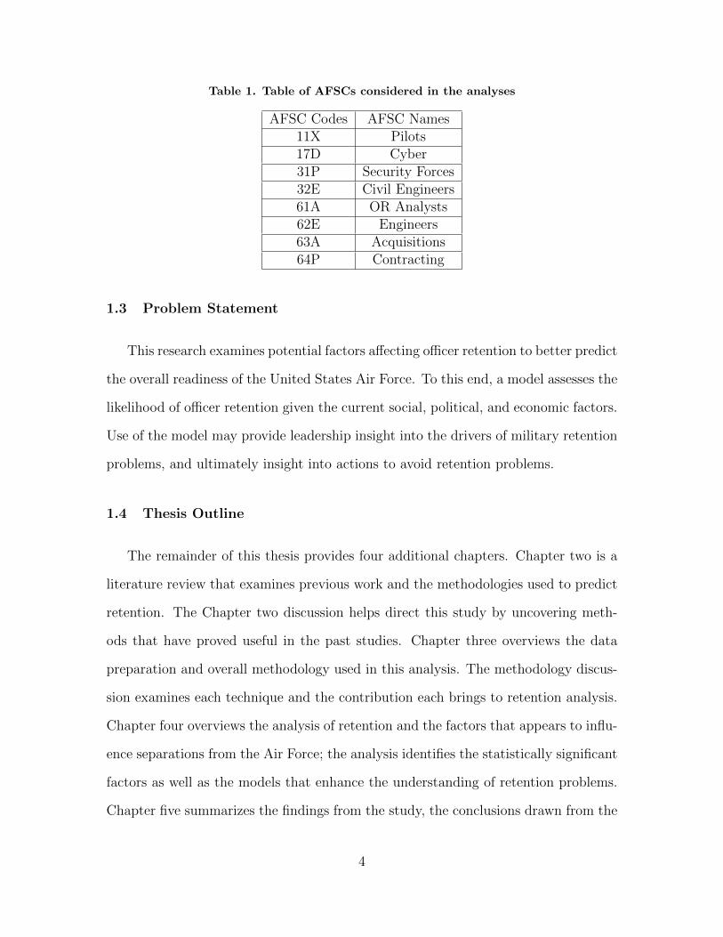
Table 1. Table of AFSCs considered in the analyses
AFSC Codes AFSC Names11X Pilots17D Cyber31P Security Forces32E Civil Engineers61A OR Analysts62E Engineers63A Acquisitions64P Contracting
1.3 Problem Statement
This research examines potential factors affecting officer retention to better predict
the overall readiness of the United States Air Force. To this end, a model assesses the
likelihood of officer retention given the current social, political, and economic factors.
Use of the model may provide leadership insight into the drivers of military retention
problems, and ultimately insight into actions to avoid retention problems.
1.4 Thesis Outline
The remainder of this thesis provides four additional chapters. Chapter two is a
literature review that examines previous work and the methodologies used to predict
retention. The Chapter two discussion helps direct this study by uncovering meth-
ods that have proved useful in the past studies. Chapter three overviews the data
preparation and overall methodology used in this analysis. The methodology discus-
sion examines each technique and the contribution each brings to retention analysis.
Chapter four overviews the analysis of retention and the factors that appears to influ-
ence separations from the Air Force; the analysis identifies the statistically significant
factors as well as the models that enhance the understanding of retention problems.
Chapter five summarizes the findings from the study, the conclusions drawn from the
4

analysis, and offers insights for leadership.
5
II. Literature Review
2.1 Overview
This section examines existing studies that pertain to Air Force retention, the
factors that seemingly affect an individual’s decision to leave the military, and the
statistical methods and metrics useful for analyzing retention. An initial review of
these studies reveals preexisting coverage of this topic and the analytical techniques
used. This allows more thorough analysis based upon the successes or failures of pre-
vious research. The literature review examines two important topics; those involving
the specific AFSC attrition and the analyses on each of these AFSCs. The specific
AFSC topic will focus on the historic and current trends of the retention rates and
emerging threats to retention. The second topic focuses on the factors that have been
effective in predicting retention and the techniques used to evaluate these factors
previously.
2.2 Military Retention Problem
The military has a unique retention problem in that it must grow its own leaders;
the military cannot direct hire its senior military leaders. Predicting attrition is valu-
able to understand and mitigate those factors that most heavily encourage separation
for military members. Every organization has competition for qualified employees and
therefore has employee turnover, but the military directly competes with the civilian
sector. Attrition results in a cost that is larger than just the cost of training new
members; it also includes the indirect costs to the unit described by morale and per-
formance [1]. Commitment is a strong component of the military’s retention issue,
but the high stress caused by deployments, relocation, and under-manning in certain
career fields increases attrition among military members [2]. While deployments and
6
certain stressors drive higher attrition, they cannot be eliminated as they are neces-
sary to military operations. Short of getting rid of deployments for Air Force officers,
there are other methods of retention programs that could be evaluated and refined
in the military. Ramlall suggests that training, rewards, career advancements, and
flexibility of work schedules can combat the attrition of individuals from an organiza-
tion [3]. Unfortunately, the freedom within the military, the merit-based promotion
structure, and job flexibility does not seem present in the military [4]. Kane argues
that the military fails to retain the most talented leaders due to the military function-
ing as a bureaucracy rather than meritocracy [4]. The civilian sector becomes more
attractive to these talented individuals where their talent may be better recognized
and the stresses of military life less realized.
2.3 Previous Efforts
This analysis is a continuation of previous research that has applied forecasting
techniques to predict attrition, particularly of two recent theses by Jantscher [5]
and Elliot [6]. Jantscher examines each AFSC and the correlation of retention by
AFSC to continuous economic data. Her study found that every AFSC, except for
chaplains and intelligence officers, had a negative correlation, showing that with a
flourishing economy, retention decreases [5]. Her findings examined total attrition in
the Air Force rather than specific AFSCs, but still provides insight as to how the
economy can affect Air Force separation rates. Certain economic factors, specific to
career fields, are useful in predicting retention. Jantscher [5] notes which factors show
patterns of correlation, but not necessarily significance. These variables are examined
and applied to this thesis in conjunction with more than just the economic factors
introduced by Jantscher [5].
In a more experimental approach, Elliot [6] tests the theory that economic factors
7
have a significant relationship to attrition using dynamic regression. Using a more
formal approach to predicting attrition, Elliot finds that Jantscher’s hypothesis, that
economic variables impact attrition, is correct [6]. Elliot uses ARIMA, exponential
smoothing, and dynamic regression approaches to forecast future attrition.
This current study expands upon Elliot’s work using similar techniques, but on
AFSC specific attrition rates. Economic stimuli have different affects on job types and
certain economic indicators are more beneficial to predicting separation for certain
AFSCs. Elliot finds that overall economic conditions impact attrition, but there is
evidence from Schofield that more than the overall economy impacts attrition by
AFSC.
Each AFSC has specific factors that influence their rates of attrition and affect
their manpower. These must be taken into account when evaluating individual AF-
SCs. Schofield et al [7] analyzes retention in the Air Force based on an individual’s
characteristics and history in the Air Force, drawing conclusions on the most and
least at risk AFSCs in terms of attrition. Their study finds that operations research
analysts had one of the most concerning retention problems, while cyberspace oper-
ators had the least retention issues of the non-rated career fields studied [7]. This
paper will focus on these two career fields to validate Schofield’s findings. Schofield’s
et al analysis is based upon survivability models using logistic regression, potentially
yielding different results than the proposed methodology of this analysis. Schofield et
al also finds that year group, gender, commission source, prior enlisted, career field,
and distinguished graduates were the most influential factors in determining retention
of an individual [7]. This analysis looks to use the information from Schofield and
build upon it using different techniques and introducing different factors predicting
retention.
8
2.4 Analytical Techniques
Linear regression is a useful technique when performing analysis to predict the
number of officers that leave the Air Force monthly. Residual analysis helps de-
termine model adequacy and goodness of fit of the model [8]. It is assumed that
residuals must maintain constant variance and normality. Empirical modeling uses
ordinary least squares regression to model relationships between input variables and
response variables. The best fit of the model is defined by minimizing the sum of
the square residuals, or differences between actual and predicted values. Analysis of
variance (ANOVA) is used to determine which parameters have the greatest influ-
ence on retention rates. ANOVA allocates to factors the total variability explained
by the model and the goodness of fit of the overall model. Since many of the input
parameters are employment numbers, and thus related, there are issues with variance
inflation. Variance inflation occurs when variables have high correlation, and causes
an over-emphasis of the significance of these variables in the model.
To reduce variance inflation, remove the factors that are causing multicollinearity.
Variable selection methods help in choosing a good set of factors. Variable selection
methods include step-wise regression or all possible models. There exists in this data
a set of “candidate predictors” as defined by Montgomery [9]. A step-wise regression
adds or removes variables from a model based on a specified criterion [9]. In this
study, the criterion used minimizes the Akaike Information Criteria (AIC) of the
model which is determined by the log-likelihood and the significance of parameters in
the model. Step-wise regression consists of a combination of forward and backward
steps that reach the minimum value of the AIC. This method can be deceived by
multicollinearity, so it is important to continuously check for multicollinearity in the
independent variables of the regression during each iteration of fitting the model.
The regression analysis leads to forecasting each variable that is found significant.
9
Research shows many potential forecasting methods can be applied to predict each
independent variable. Ultimately Box-Jenkins (ARIMA) models are chosen for time
series forecasting on the independent variables for each AFSC. ARIMA models pro-
vide the most sophisticated approach to forecasting seasonal or non-seasonal data.
This is a three step approach outlined by Thomopoulos as identification, fitting, and
diagnostic checking [10]. This is an iterative process that should meet all assumptions
of diagnostic checking as well as reducing model complexity when necessary. Tho-
mopoulos discusses the basic concepts of ARIMA models including the parameters
that shape the forecast (p,d,q) which are non-seasonal auto-regressive parameters,
differences in the data, and moving average parameters respectively. The generic
model, ARIMA(1,d,1), is altered to include more parameters in the model, but over-
specifying the model can lead to over-fitting and therefore obtaining biased forecasts.
Reducing model complexity is desired.
Diagnostic checking of ARIMA models is similar to regression. The major dif-
ference is the auto-correlation function which Thomopoulos describes as finding the
correlation of the lags and ensuring the correlations from the lags does not exceed
above or beyond a threshold related to the number of lags examined [10]. The equa-
tions for the auto-correlation function are in chapter 3 of this study.
The Box-Jenkins forecast equations are particular to the independent variables
found significant in each regression. The forecast equations differ greatly depending
on the type of model used and are expressed by Thomopoulos, but not included in this
literature review for the sake of brevity [10]. With forecasting, the future becomes
more unpredictable the further out the attempted forecasts [10]. The confidence
bounds surrounding the forecasts become much wider over time. The confidence
region informs leadership of the upper and lower expected limits for attrition in a
given month rather than a point forecast.
10
III. Methodology
3.1 Overview
This chapter discusses data collection and the sources from which the data are
obtained. The data are collected from multiple sources and compiled into a master
data set encompassing data for 67 AFSCs. This chapter highlights how the data are
prepared to create a complete data set with which we conduct analysis and draw
conclusions. Lastly, this chapter discusses the analytical techniques used to deter-
mine potential drivers of attrition. Each AFSC has idiosyncrasies within the data, so
there is no single methodology used throughout. Instead, the analytical techniques
described in this chapter cover the general approach for linear regression and forecast-
ing as well as key assumptions needed to perform the analysis. Chapter 4 discusses
in more detail the individualized analysis needed for each AFSC.
3.2 Data Description
The initial data set was provided by previous efforts on retention analysis for the
Air Force [5] [6]. The original data are obtained from the Strategic Analysis branch
of the Force Management Division of Headquarters Air Force. The separation count
measures the number of officers who left the Air Force during a given month. The
data also measures the total number of officers employed in each AFSC and the AFSC
labels. Other data includes the monthly economic indicators from October 2004 to
September 2017. The statistics included are Consumer Price Index, unemployment
rate, Gross Domestic Product per capita, median household income, and labor force
momentum. The Bureau of Economic Analysis has open source information of ac-
curate and objective economic statistics for this analysis. This creates an initial and
complete data set with 156 observations for 67 different AFSCs. While the data
11
set is complete and easily obtainable, other factors are introduced to provide better
predictions, models, and analysis.
Coupling this existing data set with AFSC specific factors may provide more
insight to leadership about the factors influencing retention. For example, pilot re-
tention could be dependent on airline hiring, but acquisitions officer retention is not
likely impacted by an increase or decrease in airline hiring. The Bureau of Labor
Statistics has employment hiring for hundreds of career fields beginning in the early
2000’s and can be applied to each specific career field within the Air Force based on
these comparable jobs in the civilian sector. Each variable introduces the raw in-
crease or decrease in employment hiring specific to certain career fields. The benefit
of using this data compared to the unemployment rate as a predictor is that it better
represents certain career fields rather than a more general approach with the unem-
ployment rate. The introduction of AFSC specific data sets to retention with general
economic conditions may aid in predicting retention more accurately and forecasting
future retention rates.
Beyond the economic scope of retention, there are other factors that may serve
as a proxy influence on retention. Political conditions shape the general outlook of a
population. Creating a proxy variable of the political climate, in terms of the pres-
ident of the United States, as either Republican or Democrat may benefit retention
prediction. Military expenditures are hypothesized to influence an individual to leave
if they see a decrease of military expenditures to occur in the upcoming years or
previous years. Given the barriers to immediate exit from the military, lags in the
data are also introduced to account for the time it takes to make the decision to leave
the Air Force and the actual date of separation.
Predicting overall retention helps to maintain total force levels for each career field,
but identifying specific individuals could also be used to predict survivability of career
12
fields and the demographics of the personnel in a career field. These demographics
include rank, which is a critical component to retention since you need senior leaders in
each career field. The addition of individual analysis would provide a more thorough
understanding of retention. Data sets, stripped of personally identifiable information,
contain information on an individual’s AFSC, marital status, years of service, and
others. Individual data is sensitive by nature and difficult to obtain, but is a critical
factor to measure the risk of separation along with the overall outlook of the economy.
While the data are available, due to constraints on time and the privacy of individual
data, the analysis of individual risk of separation is not studied here, but left for
future research.
3.3 Data Preparation
Data generally requires cleaning prior to analysis. Economic data is pulled from
the bureau of labor statistics, bureau of economic analysis, and other government
websites, and there are compatibility issues across each platform. The new data
is formatted to fit the data set containing AFSC separation count and economic
indicators.
Merging the data sets yields the final and complete data set. The AFSC data
set is recorded on the last day of each month, while the new data sets with civilian
job hiring, and military expenditures are recorded on the first day of each month.
To align dates, the new data sets dates are subtracted by one day, then matching
the initial AFSC data set. Each date entry is then transformed into ”YYYY-MM-
DD” format and merged so that every time a date is matched, it completes a single
monthly entry with all of the data employed.
Separations for each AFSC are recorded monthly, but many economic factors are
not necessarily recorded monthly. Instead of having missing values in the data, if a
13
factor is recorded every quarter, then that value is assumed the same for each month
in the quarter. The same is assumed for biannual data if it applies to one of the
independent variables. To introduce continuity in the data, and to better inform the
regression models, a 12-month, moving average is then used on the variables that were
not recorded monthly. The moving average technique smooths the data so that it is
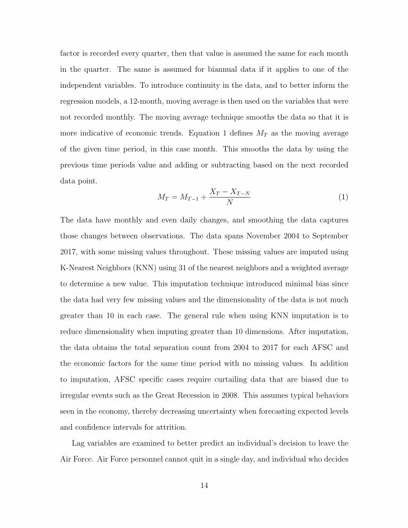
more indicative of economic trends. Equation 1 defines MT as the moving average
of the given time period, in this case month. This smooths the data by using the
previous time periods value and adding or subtracting based on the next recorded
data point.
MT = MT−1 +XT −XT−N
N(1)
The data have monthly and even daily changes, and smoothing the data captures
those changes between observations. The data spans November 2004 to September
2017, with some missing values throughout. These missing values are imputed using
K-Nearest Neighbors (KNN) using 31 of the nearest neighbors and a weighted average
to determine a new value. This imputation technique introduced minimal bias since
the data had very few missing values and the dimensionality of the data is not much
greater than 10 in each case. The general rule when using KNN imputation is to
reduce dimensionality when imputing greater than 10 dimensions. After imputation,
the data obtains the total separation count from 2004 to 2017 for each AFSC and
the economic factors for the same time period with no missing values. In addition
to imputation, AFSC specific cases require curtailing data that are biased due to
irregular events such as the Great Recession in 2008. This assumes typical behaviors
seen in the economy, thereby decreasing uncertainty when forecasting expected levels
and confidence intervals for attrition.
Lag variables are examined to better predict an individual’s decision to leave the
Air Force. Air Force personnel cannot quit in a single day, and individual who decides
14
to leave likely decides months before their actual separation date. Lag variables are
created on the separation count at six months and twelve months. This captures the
economic conditions when an individual decides to leave the Air Force and better
informs decision makers beforehand on how the certain conditions affects retention.
The master data set following the introduction of new variables and cleaning of exist-
ing data contained 4670 observations on 51 different variables. The data also consists
of 67 different AFSCs. For this analysis, 8 AFSCs were chosen based on a range of
critical manning. These AFSCs are shown in Table 1. Each AFSC is individually
analyzed to provide the most thorough results.
Lastly, for model validation purposes, the data is split to include a training and
test set. The training set comprises roughly the first 80% of the available data for
each AFSC. The last 20% of the data is held for model validation purposes to identify
the correctly predicted separations within the predicted 95% confidence bounds.
3.4 Regression Analysis
Linear regression analysis is used to assess relationships between independent and
dependent variables. Assumptions for regression must be met which include normality
of residuals as well as constant variance. Normality of residuals is checked by plotting
the difference between actual and predicted separation count from the model. The
residuals must follow a normal distribution (or at least reasonably symmetric) for valid
inferences. Constant variance means that the residuals do not vary systematically over
time, ensuring the model does not fit some observations well and others observations
poorly.
This analysis performs regression analysis on the economic indicators and the
specified civilian employment variables for each AFSC. The regression provides insight
as to which variables significantly affect officer retention in the Air Force. The research
15
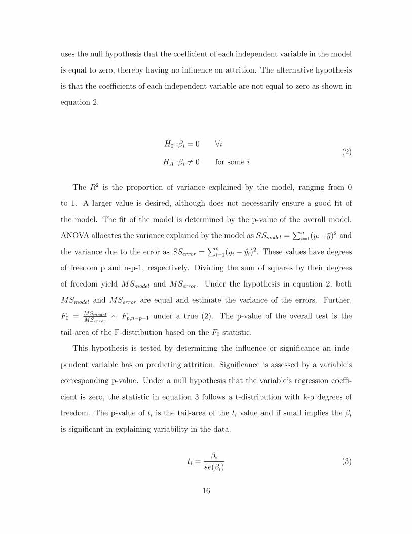
uses the null hypothesis that the coefficient of each independent variable in the model
is equal to zero, thereby having no influence on attrition. The alternative hypothesis
is that the coefficients of each independent variable are not equal to zero as shown in
equation 2.
H0 :βi = 0 ∀i
HA :βi 6= 0 for some i
(2)
The R2 is the proportion of variance explained by the model, ranging from 0
to 1. A larger value is desired, although does not necessarily ensure a good fit of
the model. The fit of the model is determined by the p-value of the overall model.
ANOVA allocates the variance explained by the model as SSmodel =∑n
i=1(yi−y)2 and
the variance due to the error as SSerror =∑n
i=1(yi − yi)2. These values have degrees
of freedom p and n-p-1, respectively. Dividing the sum of squares by their degrees
of freedom yield MSmodel and MSerror. Under the hypothesis in equation 2, both
MSmodel and MSerror are equal and estimate the variance of the errors. Further,
F0 = MSmodel
MSerror∼ Fp,n−p−1 under a true (2). The p-value of the overall test is the
tail-area of the F-distribution based on the F0 statistic.
This hypothesis is tested by determining the influence or significance an inde-
pendent variable has on predicting attrition. Significance is assessed by a variable’s
corresponding p-value. Under a null hypothesis that the variable’s regression coeffi-
cient is zero, the statistic in equation 3 follows a t-distribution with k-p degrees of
freedom. The p-value of ti is the tail-area of the ti value and if small implies the βi
is significant in explaining variability in the data.
ti =βi
se(βi)(3)
16
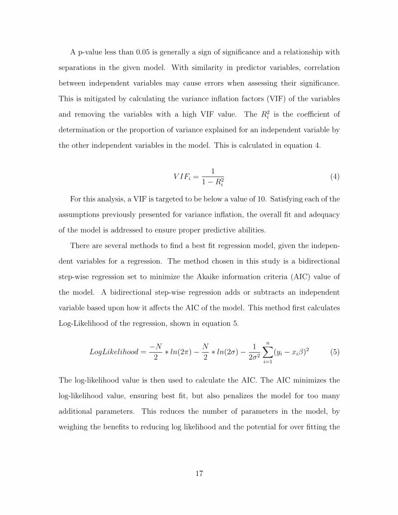
A p-value less than 0.05 is generally a sign of significance and a relationship with
separations in the given model. With similarity in predictor variables, correlation
between independent variables may cause errors when assessing their significance.
This is mitigated by calculating the variance inflation factors (VIF) of the variables
and removing the variables with a high VIF value. The R2i is the coefficient of
determination or the proportion of variance explained for an independent variable by
the other independent variables in the model. This is calculated in equation 4.
V IFi =1
1−R2i
(4)
For this analysis, a VIF is targeted to be below a value of 10. Satisfying each of the
assumptions previously presented for variance inflation, the overall fit and adequacy
of the model is addressed to ensure proper predictive abilities.
There are several methods to find a best fit regression model, given the indepen-
dent variables for a regression. The method chosen in this study is a bidirectional
step-wise regression set to minimize the Akaike information criteria (AIC) value of
the model. A bidirectional step-wise regression adds or subtracts an independent
variable based upon how it affects the AIC of the model. This method first calculates
Log-Likelihood of the regression, shown in equation 5.
LogLikelihood =−N
2∗ ln(2π)− N
2∗ ln(2σ)− 1
2σ2
n∑i=1
(yi − xiβ)2 (5)
The log-likelihood value is then used to calculate the AIC. The AIC minimizes the
log-likelihood value, ensuring best fit, but also penalizes the model for too many
additional parameters. This reduces the number of parameters in the model, by
weighing the benefits to reducing log likelihood and the potential for over fitting the
17
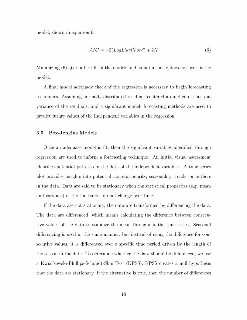
model, shown in equation 6.
AIC = −2(LogLikelihood) + 2K (6)
Minimizing (6) gives a best fit of the models and simultaneously does not over fit the
model.
A final model adequacy check of the regression is necessary to begin forecasting
techniques. Assuming normally distributed residuals centered around zero, constant
variance of the residuals, and a significant model, forecasting methods are used to
predict future values of the independent variables in the regression.
3.5 Box-Jenkins Models
Once an adequate model is fit, then the significant variables identified through
regression are used to inform a forecasting technique. An initial visual assessment
identifies potential patterns in the data of the independent variables. A time series
plot provides insights into potential non-stationarity, seasonality trends, or outliers
in the data. Data are said to be stationary when the statistical properties (e.g. mean
and variance) of the time series do not change over time.
If the data are not stationary, the data are transformed by differencing the data.
The data are differenced, which means calculating the difference between consecu-
tive values of the data to stabilize the mean throughout the time series. Seasonal
differencing is used in the same manner, but instead of using the difference for con-
secutive values, it is differenced over a specific time period driven by the length of
the season in the data. To determine whether the data should be differenced, we use
a Kwiatkowski-Phillips-Schmidt-Shin Test (KPSS). KPSS creates a null hypothesis
that the data are stationary. If the alternative is true, then the number of differences
18
is calculated and applied to the data to establish stationarity.
With non-stationary data in the variance of the data, transformations are applied,
such as the log function or square root. Seasonality is determined through visual
inspection of the data or expert knowledge of the data. Lastly, before analysis,
identifying and manipulating outliers is necessary for certain AFSCs to have a more
accurate model. Outliers are either smoothed using a moving average or removed
from the data entirely for the purposes of this analysis.
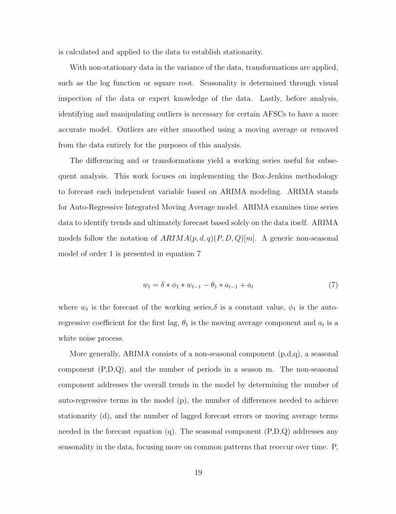
The differencing and or transformations yield a working series useful for subse-
quent analysis. This work focuses on implementing the Box-Jenkins methodology
to forecast each independent variable based on ARIMA modeling. ARIMA stands
for Auto-Regressive Integrated Moving Average model. ARIMA examines time series
data to identify trends and ultimately forecast based solely on the data itself. ARIMA
models follow the notation of ARIMA(p, d, q)(P,D,Q)[m]. A generic non-seasonal
model of order 1 is presented in equation 7
wt = δ ∗ φ1 ∗ wt−1 − θ1 ∗ at−1 + at (7)
where wt is the forecast of the working series,δ is a constant value, φ1 is the auto-
regressive coefficient for the first lag, θ1 is the moving average component and at is a
white noise process.
More generally, ARIMA consists of a non-seasonal component (p,d,q), a seasonal
component (P,D,Q), and the number of periods in a season m. The non-seasonal
component addresses the overall trends in the model by determining the number of
auto-regressive terms in the model (p), the number of differences needed to achieve
stationarity (d), and the number of lagged forecast errors or moving average terms
needed in the forecast equation (q). The seasonal component (P,D,Q) addresses any
seasonality in the data, focusing more on common patterns that reoccur over time. P,
19
D, and Q represent the same respective parameters in the non-seasonal component,
but help to shape these reoccurring trends within the data. An example of a non-
seasonal model would be world population, always increasing over time. An example
of a seasonal model would be a sinusoidal curve, that follows a similar trend over
time. Lastly, the number of periods in a season [m] is typically determined by the
type of data the model is fitting. Attrition is measured monthly, so the number of
periods in a season is 12 months. The combination of these components helps shape
the data and extrapolate beyond the time series. The forecast provides an expected
value as well as 80 percent and 95 percent confidence regions for each independent
variable used to predict attrition.
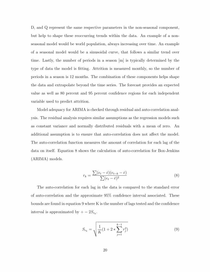
Model adequacy for ARIMA is checked through residual and auto-correlation anal-
ysis. The residual analysis requires similar assumptions as the regression models such
as constant variance and normally distributed residuals with a mean of zero. An
additional assumption is to ensure that auto-correlation does not affect the model.
The auto-correlation function measures the amount of correlation for each lag of the
data on itself. Equation 8 shows the calculation of auto-correlation for Box-Jenkins
(ARIMA) models.
rk =
∑(et − e)(et−k − e)∑
(et − e)2(8)
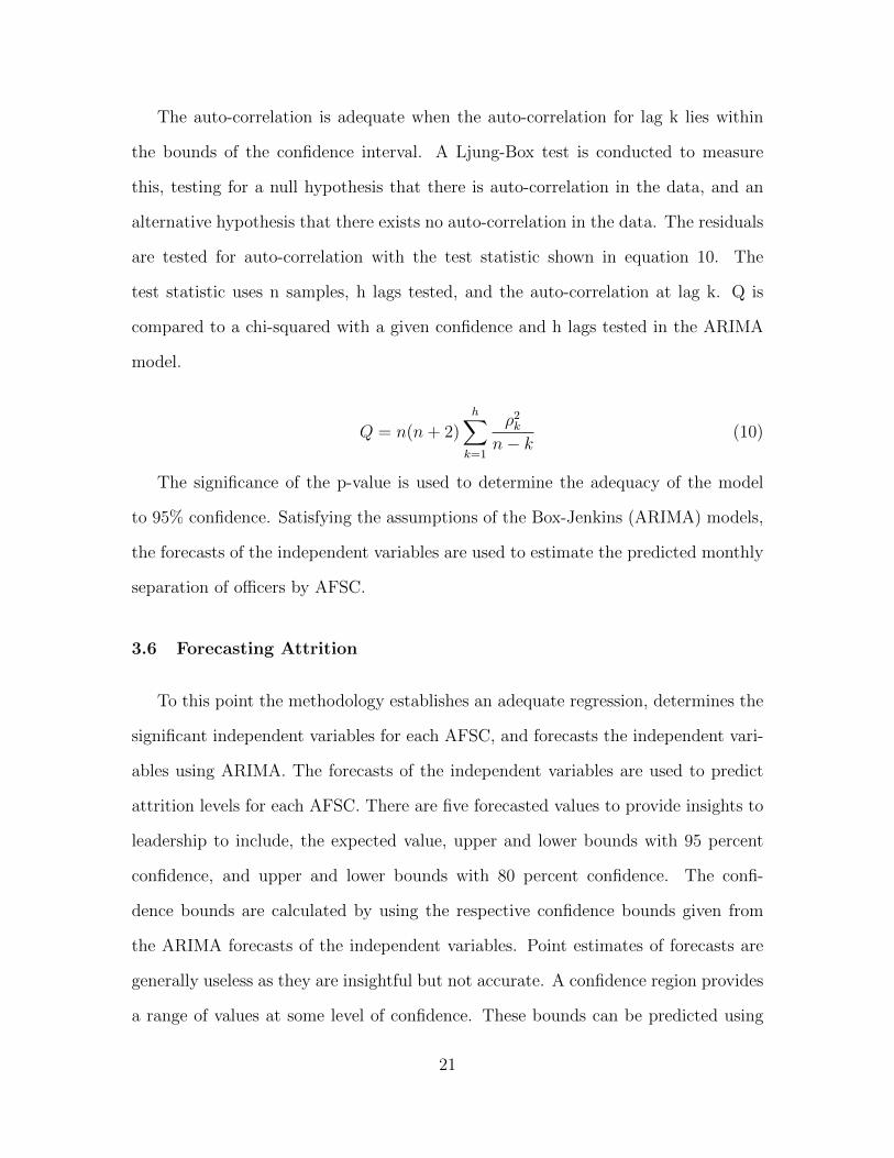
The auto-correlation for each lag in the data is compared to the standard error
of auto-correlation and the approximate 95% confidence interval associated. These
bounds are found in equation 9 where K is the number of lags tested and the confidence
interval is approximated by +− 2Srk .
Srk =
√√√√ 1
K(1 + 2 ∗
k−1∑j=1
r2j ) (9)
20
The auto-correlation is adequate when the auto-correlation for lag k lies within
the bounds of the confidence interval. A Ljung-Box test is conducted to measure
this, testing for a null hypothesis that there is auto-correlation in the data, and an
alternative hypothesis that there exists no auto-correlation in the data. The residuals
are tested for auto-correlation with the test statistic shown in equation 10. The
test statistic uses n samples, h lags tested, and the auto-correlation at lag k. Q is
compared to a chi-squared with a given confidence and h lags tested in the ARIMA
model.
Q = n(n+ 2)h∑k=1
ρ2kn− k
(10)
The significance of the p-value is used to determine the adequacy of the model
to 95% confidence. Satisfying the assumptions of the Box-Jenkins (ARIMA) models,
the forecasts of the independent variables are used to estimate the predicted monthly
separation of officers by AFSC.
3.6 Forecasting Attrition
To this point the methodology establishes an adequate regression, determines the
significant independent variables for each AFSC, and forecasts the independent vari-
ables using ARIMA. The forecasts of the independent variables are used to predict
attrition levels for each AFSC. There are five forecasted values to provide insights to
leadership to include, the expected value, upper and lower bounds with 95 percent
confidence, and upper and lower bounds with 80 percent confidence. The confi-
dence bounds are calculated by using the respective confidence bounds given from
the ARIMA forecasts of the independent variables. Point estimates of forecasts are
generally useless as they are insightful but not accurate. A confidence region provides
a range of values at some level of confidence. These bounds can be predicted using
21
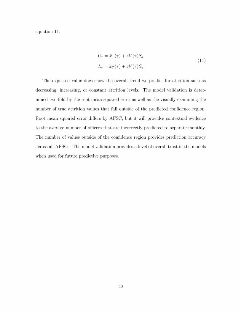
equation 11.
Uτ = xT (τ) + zV (τ)Sa
Lτ = xT (τ) + zV (τ)Sa
(11)
The expected value does show the overall trend we predict for attrition such as
decreasing, increasing, or constant attrition levels. The model validation is deter-
mined two-fold by the root mean squared error as well as the visually examining the
number of true attrition values that fall outside of the predicted confidence region.
Root mean squared error differs by AFSC, but it will provides contextual evidence
to the average number of officers that are incorrectly predicted to separate monthly.
The number of values outside of the confidence region provides prediction accuracy
across all AFSCs. The model validation provides a level of overall trust in the models
when used for future predictive purposes.
22
IV. Analysis
4.1 Introduction
This chapter presents the analysis individually on each of the eight selected AF-
SCs, ultimately providing insight on estimated attrition levels and confidence bounds
on the AFSC specific personnel separation. Multiple linear regression is used to pre-
dict attrition and establish key regressors for attrition. Forecasts on the previously
identified regressors are used to inform the regression model to provide key insights
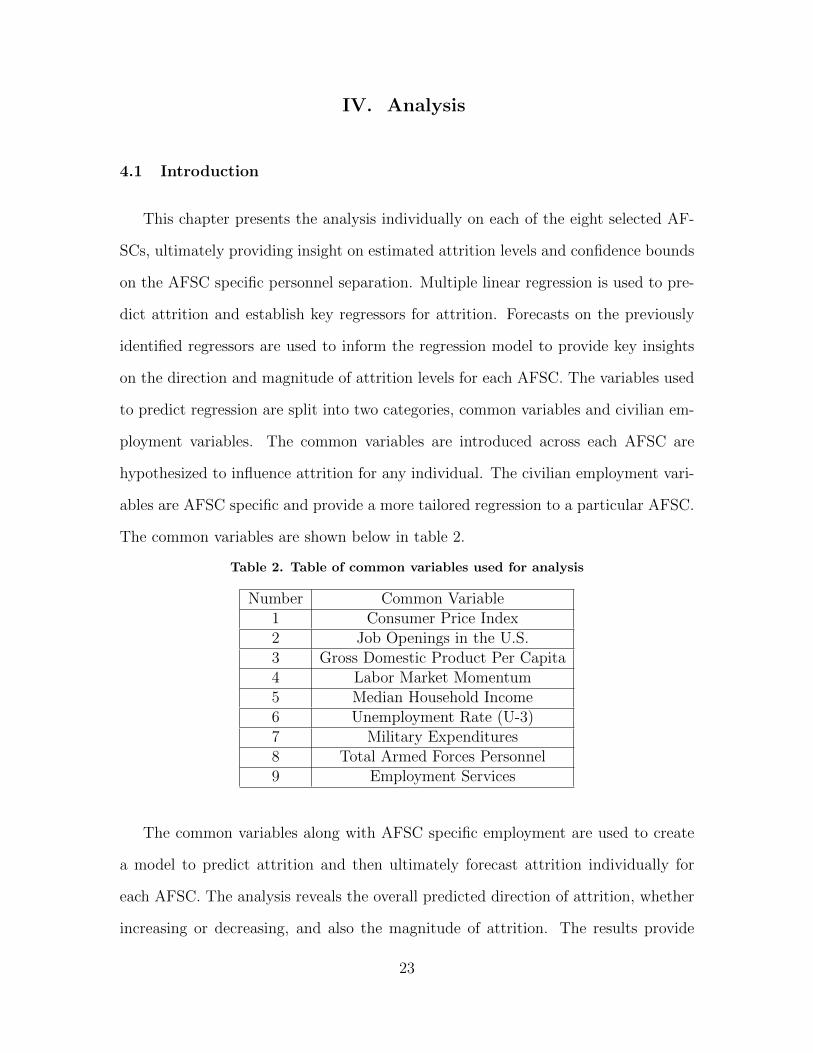
on the direction and magnitude of attrition levels for each AFSC. The variables used
to predict regression are split into two categories, common variables and civilian em-
ployment variables. The common variables are introduced across each AFSC are
hypothesized to influence attrition for any individual. The civilian employment vari-
ables are AFSC specific and provide a more tailored regression to a particular AFSC.
The common variables are shown below in table 2.
Table 2. Table of common variables used for analysis
Number Common Variable1 Consumer Price Index2 Job Openings in the U.S.3 Gross Domestic Product Per Capita4 Labor Market Momentum5 Median Household Income6 Unemployment Rate (U-3)7 Military Expenditures8 Total Armed Forces Personnel9 Employment Services
The common variables along with AFSC specific employment are used to create
a model to predict attrition and then ultimately forecast attrition individually for
each AFSC. The analysis reveals the overall predicted direction of attrition, whether
increasing or decreasing, and also the magnitude of attrition. The results provide
23
insight into recruitment, incentive programs, and assignment processes for the near
future. In each analysis, the last two years of data are withheld as validation data.
4.2 11X - Pilot Career Field Analysis
4.2.1 Regression Analysis of Pilot Career Field
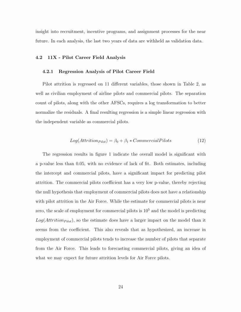
Pilot attrition is regressed on 11 different variables, those shown in Table 2, as
well as civilian employment of airline pilots and commercial pilots. The separation
count of pilots, along with the other AFSCs, requires a log transformation to better
normalize the residuals. A final resulting regression is a simple linear regression with
the independent variable as commercial pilots.
Log(AttritionPilot) = β0 + β1 ∗ CommercialP ilots (12)
The regression results in figure 1 indicate the overall model is significant with
a p-value less than 0.05, with no evidence of lack of fit. Both estimates, including
the intercept and commercial pilots, have a significant impact for predicting pilot
attrition. The commercial pilots coefficient has a very low p-value, thereby rejecting
the null hypothesis that employment of commercial pilots does not have a relationship
with pilot attrition in the Air Force. While the estimate for commercial pilots is near
zero, the scale of employment for commercial pilots is 105 and the model is predicting
Log(AttritionPilot), so the estimate does have a larger impact on the model than it
seems from the coefficient. This also reveals that as hypothesized, an increase in
employment of commercial pilots tends to increase the number of pilots that separate
from the Air Force. This leads to forecasting commercial pilots, giving an idea of
what we may expect for future attrition levels for Air Force pilots.
24
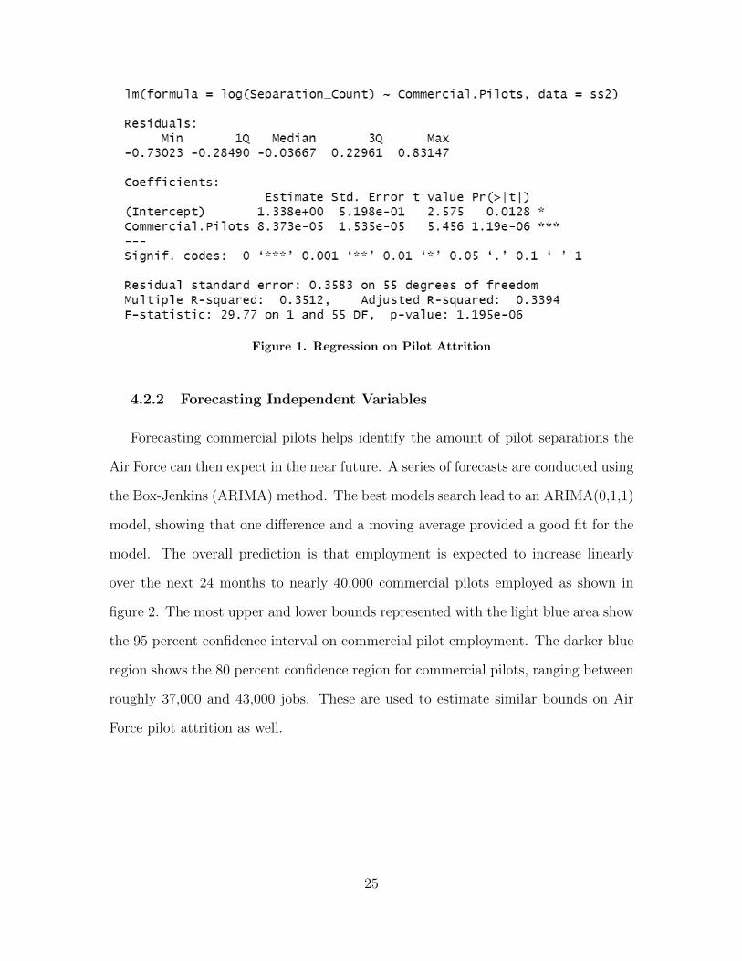
Figure 1. Regression on Pilot Attrition
4.2.2 Forecasting Independent Variables
Forecasting commercial pilots helps identify the amount of pilot separations the
Air Force can then expect in the near future. A series of forecasts are conducted using
the Box-Jenkins (ARIMA) method. The best models search lead to an ARIMA(0,1,1)
model, showing that one difference and a moving average provided a good fit for the
model. The overall prediction is that employment is expected to increase linearly
over the next 24 months to nearly 40,000 commercial pilots employed as shown in
figure 2. The most upper and lower bounds represented with the light blue area show
the 95 percent confidence interval on commercial pilot employment. The darker blue
region shows the 80 percent confidence region for commercial pilots, ranging between
roughly 37,000 and 43,000 jobs. These are used to estimate similar bounds on Air
Force pilot attrition as well.
25
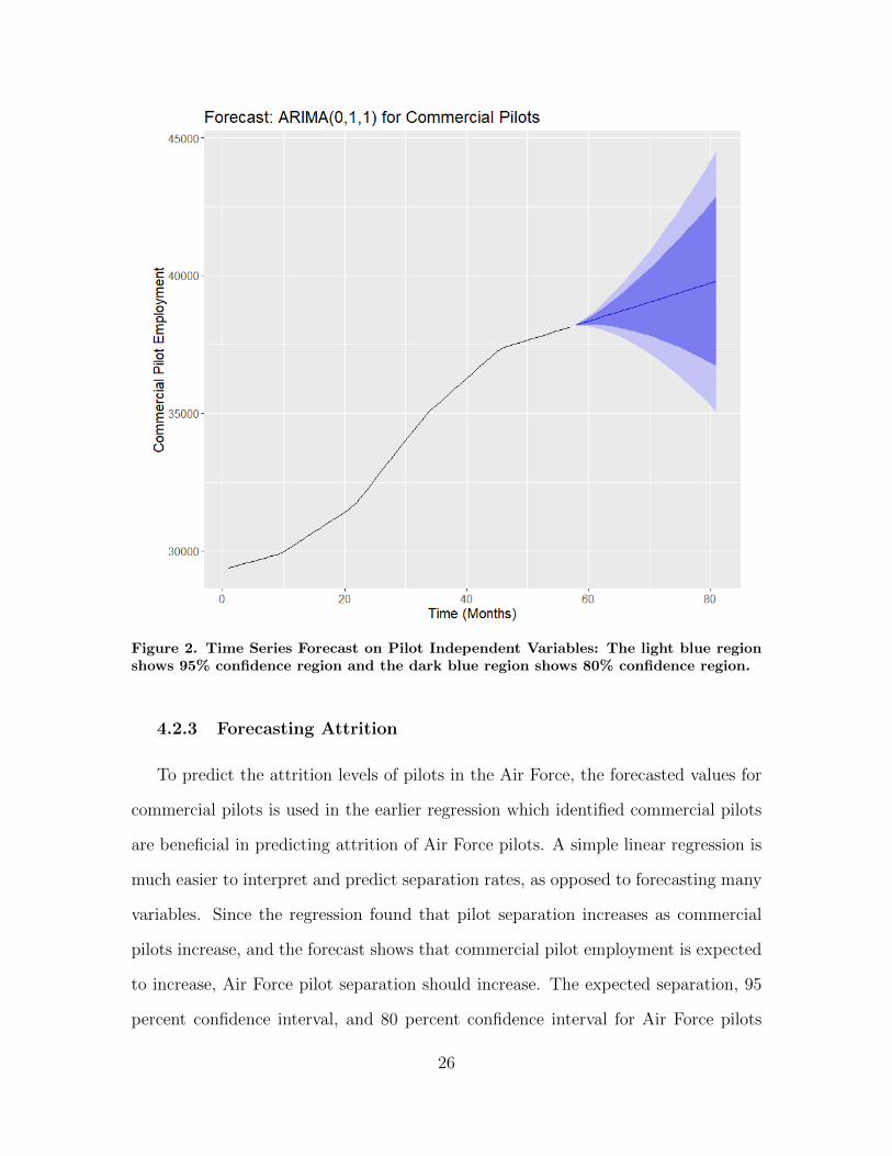
Figure 2. Time Series Forecast on Pilot Independent Variables: The light blue regionshows 95% confidence region and the dark blue region shows 80% confidence region.
4.2.3 Forecasting Attrition
To predict the attrition levels of pilots in the Air Force, the forecasted values for
commercial pilots is used in the earlier regression which identified commercial pilots
are beneficial in predicting attrition of Air Force pilots. A simple linear regression is
much easier to interpret and predict separation rates, as opposed to forecasting many
variables. Since the regression found that pilot separation increases as commercial
pilots increase, and the forecast shows that commercial pilot employment is expected
to increase, Air Force pilot separation should increase. The expected separation, 95
percent confidence interval, and 80 percent confidence interval for Air Force pilots
26
are shown in figure 3. Over the next two years, we might expect attrition to increase
from 95 to 105 pilots per month with the accompanying confidence regions. The 95%
confidence region contains 8 of 24 forecasted separations when compared with the
test data, being 33% accurate. Appendix A contains details on this model.
Figure 3. Forecast of Pilot Attrition
4.3 17D - Cyber Career Field Analysis
4.3.1 Regression Analysis of Cyber Career Field
The cyber career field growth has been more emphasized as technology increases
and becomes weaponized. Retaining personnel in the cyber career field is critical in
27
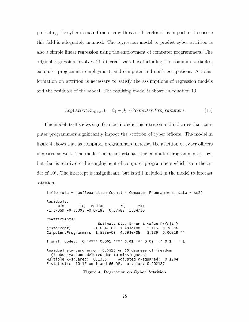
protecting the cyber domain from enemy threats. Therefore it is important to ensure
this field is adequately manned. The regression model to predict cyber attrition is
also a simple linear regression using the employment of computer programmers. The
original regression involves 11 different variables including the common variables,
computer programmer employment, and computer and math occupations. A trans-
formation on attrition is necessary to satisfy the assumptions of regression models
and the residuals of the model. The resulting model is shown in equation 13.
Log(AttritionCyber) = β0 + β1 ∗ Computer.Programmers (13)
The model itself shows significance in predicting attrition and indicates that com-
puter programmers significantly impact the attrition of cyber officers. The model in
figure 4 shows that as computer programmers increase, the attrition of cyber officers
increases as well. The model coefficient estimate for computer programmers is low,
but that is relative to the employment of computer programmers which is on the or-
der of 106. The intercept is insignificant, but is still included in the model to forecast
attrition.
Figure 4. Regression on Cyber Attrition
28
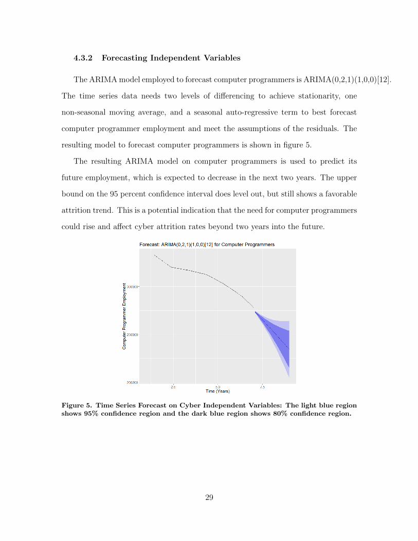
4.3.2 Forecasting Independent Variables
The ARIMA model employed to forecast computer programmers is ARIMA(0,2,1)(1,0,0)[12].
The time series data needs two levels of differencing to achieve stationarity, one
non-seasonal moving average, and a seasonal auto-regressive term to best forecast
computer programmer employment and meet the assumptions of the residuals. The
resulting model to forecast computer programmers is shown in figure 5.
The resulting ARIMA model on computer programmers is used to predict its
future employment, which is expected to decrease in the next two years. The upper
bound on the 95 percent confidence interval does level out, but still shows a favorable
attrition trend. This is a potential indication that the need for computer programmers
could rise and affect cyber attrition rates beyond two years into the future.
Figure 5. Time Series Forecast on Cyber Independent Variables: The light blue regionshows 95% confidence region and the dark blue region shows 80% confidence region.
29
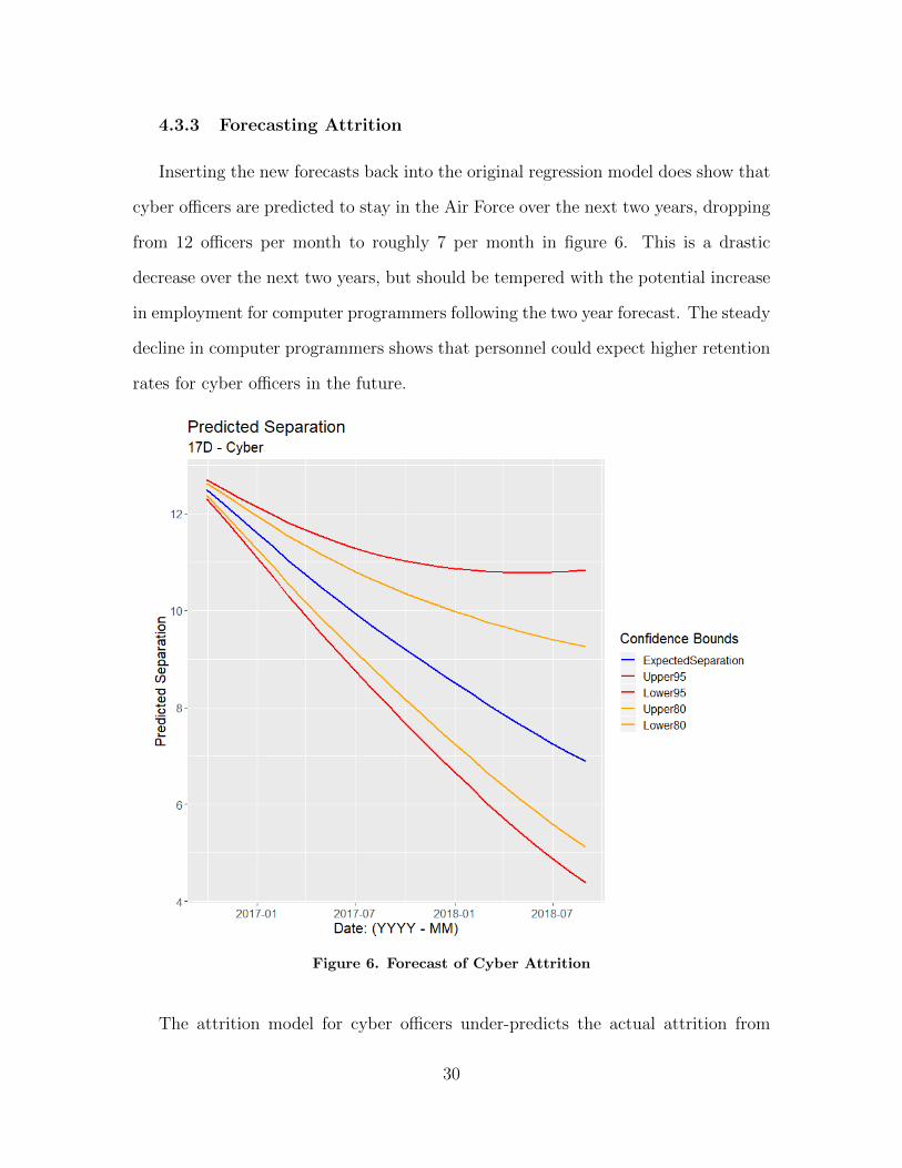
4.3.3 Forecasting Attrition
Inserting the new forecasts back into the original regression model does show that
cyber officers are predicted to stay in the Air Force over the next two years, dropping
from 12 officers per month to roughly 7 per month in figure 6. This is a drastic
decrease over the next two years, but should be tempered with the potential increase
in employment for computer programmers following the two year forecast. The steady
decline in computer programmers shows that personnel could expect higher retention
rates for cyber officers in the future.
Figure 6. Forecast of Cyber Attrition
The attrition model for cyber officers under-predicts the actual attrition from
30
2015 to 2017. The 95% confidence region contains only 3 of 24 forecasted separations
when compared with the test data, being 12.5% accurate. While this may not seem
accurate, the model follows the overall trend of the test data, shown in Appendix B.
The root mean squared error is 10, but this value is misleading since there are three
months that have abnormally large attrition levels biasing the root mean squared
error more than the typical error in prediction.
4.4 31P - Security Forces Career Field Analysis
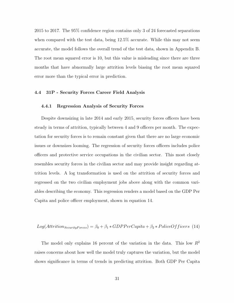
4.4.1 Regression Analysis of Security Forces
Despite downsizing in late 2014 and early 2015, security forces officers have been
steady in terms of attrition, typically between 4 and 9 officers per month. The expec-
tation for security forces is to remain constant given that there are no large economic
issues or downsizes looming. The regression of security forces officers includes police
officers and protective service occupations in the civilian sector. This most closely
resembles security forces in the civilian sector and may provide insight regarding at-
trition levels. A log transformation is used on the attrition of security forces and
regressed on the two civilian employment jobs above along with the common vari-
ables describing the economy. This regression renders a model based on the GDP Per
Capita and police officer employment, shown in equation 14.
Log(AttritionSecurityForces) = β0 + β1 ∗GDPPerCapita+ β2 ∗PoliceOfficers (14)
The model only explains 16 percent of the variation in the data. This low R2
raises concerns about how well the model truly captures the variation, but the model
shows significance in terms of trends in predicting attrition. Both GDP Per Capita
31
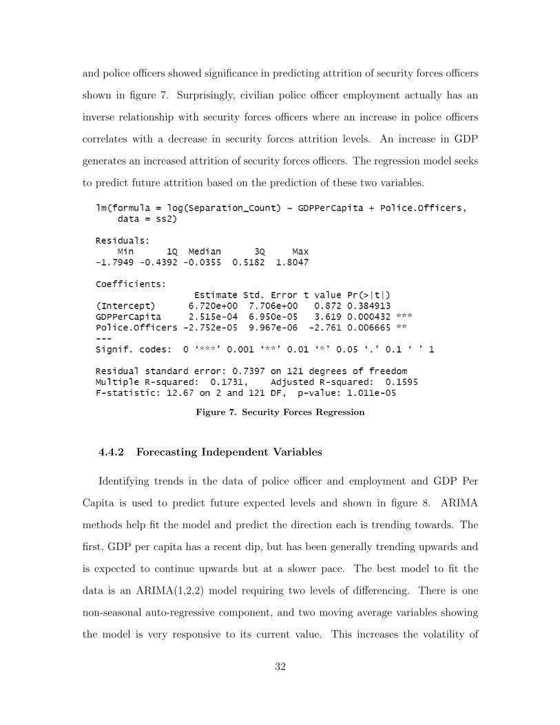
and police officers showed significance in predicting attrition of security forces officers
shown in figure 7. Surprisingly, civilian police officer employment actually has an
inverse relationship with security forces officers where an increase in police officers
correlates with a decrease in security forces attrition levels. An increase in GDP
generates an increased attrition of security forces officers. The regression model seeks
to predict future attrition based on the prediction of these two variables.
Figure 7. Security Forces Regression
4.4.2 Forecasting Independent Variables
Identifying trends in the data of police officer and employment and GDP Per
Capita is used to predict future expected levels and shown in figure 8. ARIMA
methods help fit the model and predict the direction each is trending towards. The
first, GDP per capita has a recent dip, but has been generally trending upwards and
is expected to continue upwards but at a slower pace. The best model to fit the
data is an ARIMA(1,2,2) model requiring two levels of differencing. There is one
non-seasonal auto-regressive component, and two moving average variables showing
the model is very responsive to its current value. This increases the volatility of
32
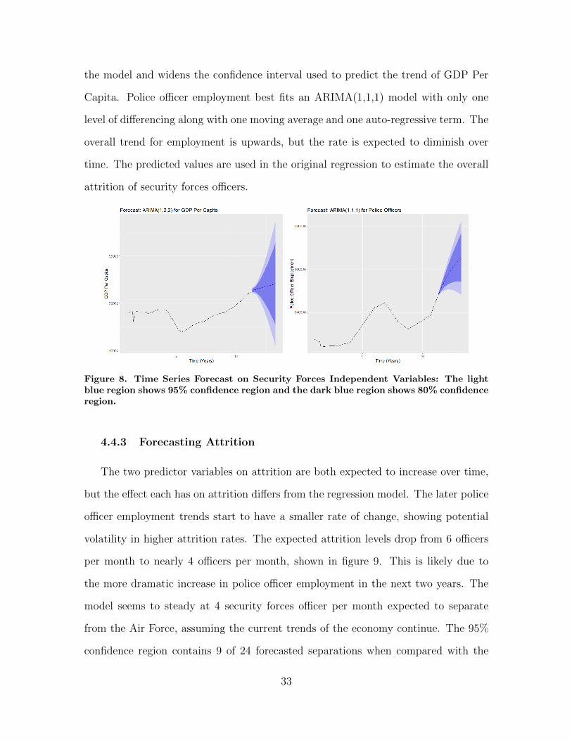
the model and widens the confidence interval used to predict the trend of GDP Per
Capita. Police officer employment best fits an ARIMA(1,1,1) model with only one
level of differencing along with one moving average and one auto-regressive term. The
overall trend for employment is upwards, but the rate is expected to diminish over
time. The predicted values are used in the original regression to estimate the overall
attrition of security forces officers.
Figure 8. Time Series Forecast on Security Forces Independent Variables: The lightblue region shows 95% confidence region and the dark blue region shows 80% confidenceregion.
4.4.3 Forecasting Attrition
The two predictor variables on attrition are both expected to increase over time,
but the effect each has on attrition differs from the regression model. The later police
officer employment trends start to have a smaller rate of change, showing potential
volatility in higher attrition rates. The expected attrition levels drop from 6 officers
per month to nearly 4 officers per month, shown in figure 9. This is likely due to
the more dramatic increase in police officer employment in the next two years. The
model seems to steady at 4 security forces officer per month expected to separate
from the Air Force, assuming the current trends of the economy continue. The 95%
confidence region contains 9 of 24 forecasted separations when compared with the
33
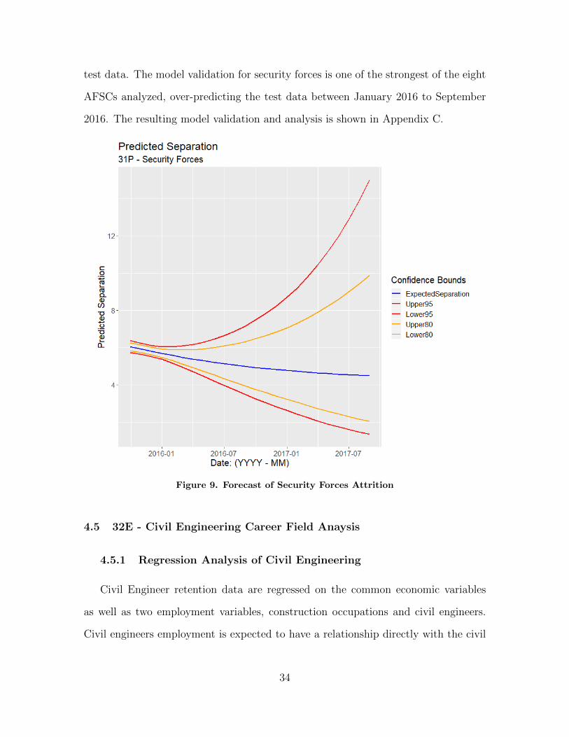
test data. The model validation for security forces is one of the strongest of the eight
AFSCs analyzed, over-predicting the test data between January 2016 to September
2016. The resulting model validation and analysis is shown in Appendix C.
Figure 9. Forecast of Security Forces Attrition
4.5 32E - Civil Engineering Career Field Anaysis
4.5.1 Regression Analysis of Civil Engineering
Civil Engineer retention data are regressed on the common economic variables
as well as two employment variables, construction occupations and civil engineers.
Civil engineers employment is expected to have a relationship directly with the civil
34
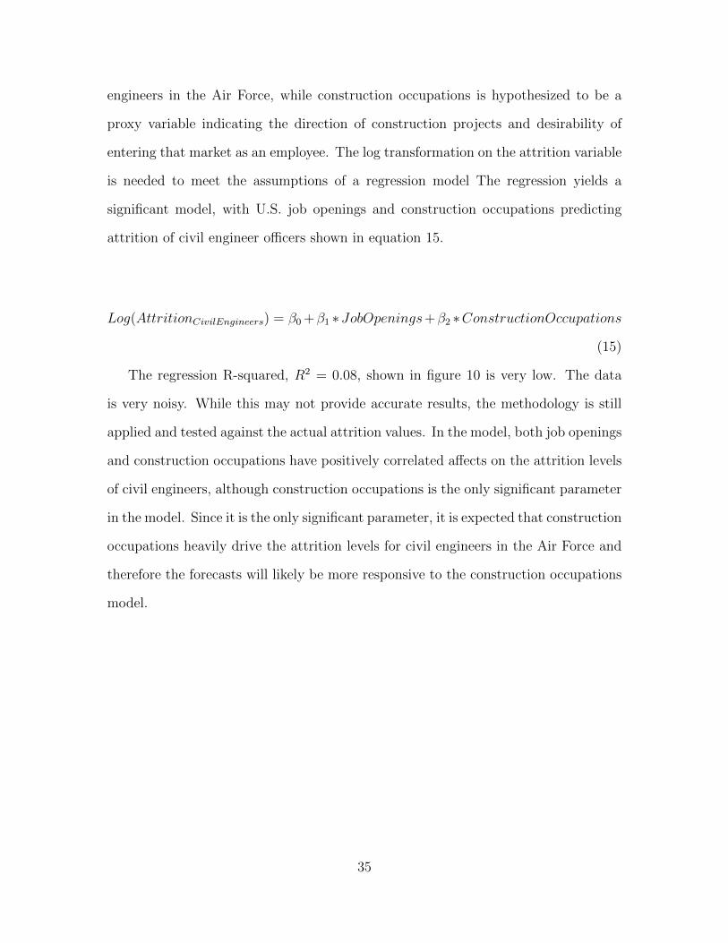
engineers in the Air Force, while construction occupations is hypothesized to be a
proxy variable indicating the direction of construction projects and desirability of
entering that market as an employee. The log transformation on the attrition variable
is needed to meet the assumptions of a regression model The regression yields a
significant model, with U.S. job openings and construction occupations predicting
attrition of civil engineer officers shown in equation 15.
Log(AttritionCivilEngineers) = β0 +β1 ∗JobOpenings+β2 ∗ConstructionOccupations
(15)
The regression R-squared, R2 = 0.08, shown in figure 10 is very low. The data
is very noisy. While this may not provide accurate results, the methodology is still
applied and tested against the actual attrition values. In the model, both job openings
and construction occupations have positively correlated affects on the attrition levels
of civil engineers, although construction occupations is the only significant parameter
in the model. Since it is the only significant parameter, it is expected that construction
occupations heavily drive the attrition levels for civil engineers in the Air Force and
therefore the forecasts will likely be more responsive to the construction occupations
model.
35
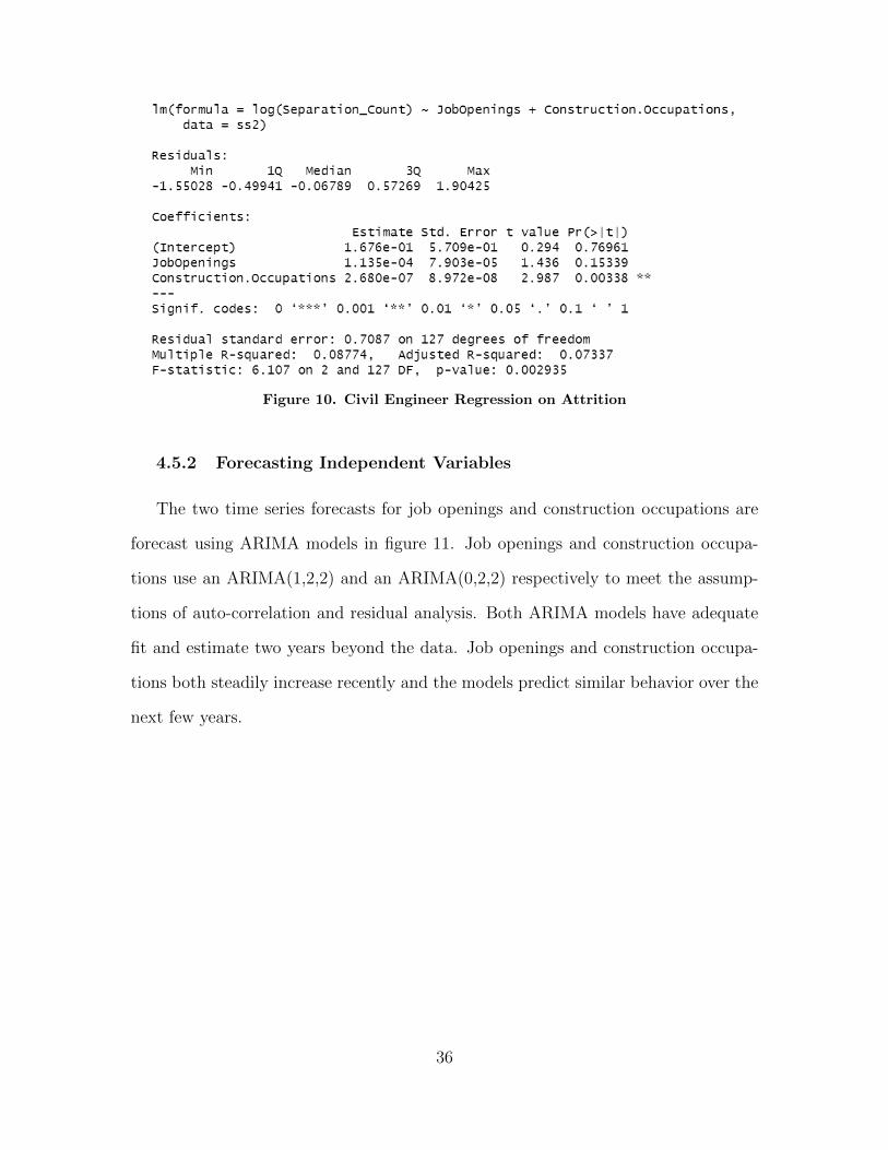
Figure 10. Civil Engineer Regression on Attrition
4.5.2 Forecasting Independent Variables
The two time series forecasts for job openings and construction occupations are
forecast using ARIMA models in figure 11. Job openings and construction occupa-
tions use an ARIMA(1,2,2) and an ARIMA(0,2,2) respectively to meet the assump-
tions of auto-correlation and residual analysis. Both ARIMA models have adequate
fit and estimate two years beyond the data. Job openings and construction occupa-
tions both steadily increase recently and the models predict similar behavior over the
next few years.
36
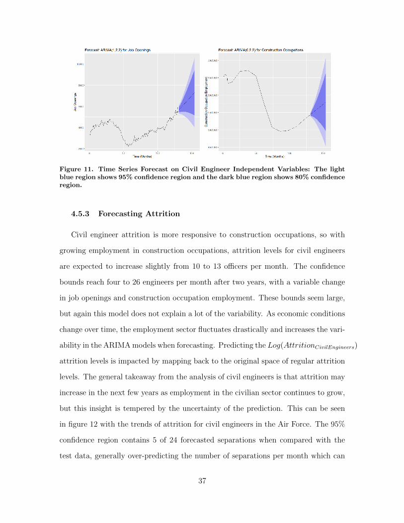
Figure 11. Time Series Forecast on Civil Engineer Independent Variables: The lightblue region shows 95% confidence region and the dark blue region shows 80% confidenceregion.
4.5.3 Forecasting Attrition
Civil engineer attrition is more responsive to construction occupations, so with
growing employment in construction occupations, attrition levels for civil engineers
are expected to increase slightly from 10 to 13 officers per month. The confidence
bounds reach four to 26 engineers per month after two years, with a variable change
in job openings and construction occupation employment. These bounds seem large,
but again this model does not explain a lot of the variability. As economic conditions
change over time, the employment sector fluctuates drastically and increases the vari-
ability in the ARIMA models when forecasting. Predicting the Log(AttritionCivilEngineers)
attrition levels is impacted by mapping back to the original space of regular attrition
levels. The general takeaway from the analysis of civil engineers is that attrition may
increase in the next few years as employment in the civilian sector continues to grow,
but this insight is tempered by the uncertainty of the prediction. This can be seen
in figure 12 with the trends of attrition for civil engineers in the Air Force. The 95%
confidence region contains 5 of 24 forecasted separations when compared with the
test data, generally over-predicting the number of separations per month which can
37
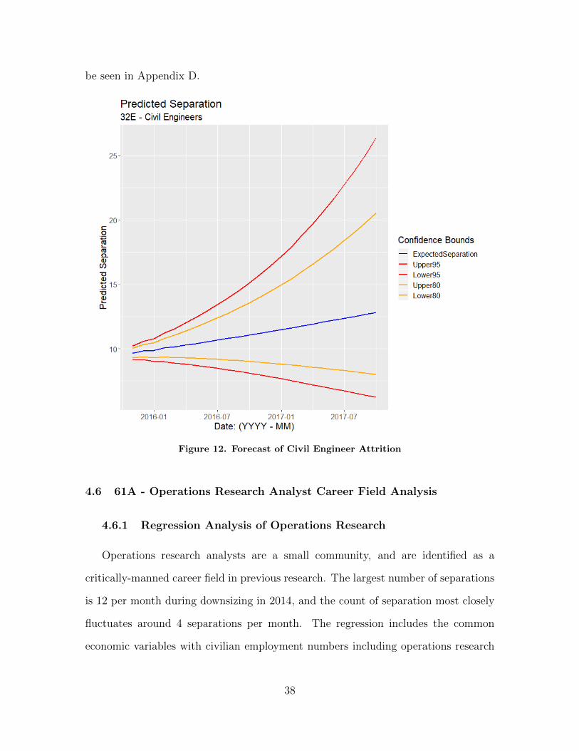
be seen in Appendix D.
Figure 12. Forecast of Civil Engineer Attrition
4.6 61A - Operations Research Analyst Career Field Analysis
4.6.1 Regression Analysis of Operations Research
Operations research analysts are a small community, and are identified as a
critically-manned career field in previous research. The largest number of separations
is 12 per month during downsizing in 2014, and the count of separation most closely
fluctuates around 4 separations per month. The regression includes the common
economic variables with civilian employment numbers including operations research
38
analysts, management occupations, business and financial operations occupations,
budget analysts, and financial analysts. Analysts have a wide range of occupations
that they can enter in the civilian sector. Thus, identifying a single job proves difficult
to predict attrition of OR analysts. A log transformation is performed on attrition to
correct residuals. The model finds that employment in services is the sole predictor
with minimal AIC. Employment in services is a very broad employment statistic pro-
vided by the Bureau of Labor Statistics which includes education, government, trade,
financial activities and many more. The equation for the resulting model is shown in
equation 16.
Log(AttritionAnalyst) = β0 + β1 ∗ EmploymentinServices (16)
The intercept at a value of 235 is concerning, along with an R-squared of around
10 percent explanation of the variance in the data. The resulting model for OR
analysts is shown in figure 13. The value of the coefficient for employment in services
is negative and therefore suggests that an increase in employment in services will
increase retention rates. The more jobs added to services correlates to more officers
deciding to remain in the Air Force, the opposite of the intuitive thoughts associated
with this correlation. It is typically expected that increasing jobs in the civilian
sector appeals of officers that separate from the military. Despite the odd values of
the coefficients, the model has adequate residuals, significant results, and significant
predictor variables.
39
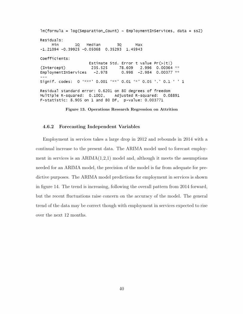
Figure 13. Operations Research Regression on Attrition
4.6.2 Forecasting Independent Variables
Employment in services takes a large drop in 2012 and rebounds in 2014 with a
continual increase to the present data. The ARIMA model used to forecast employ-
ment in services is an ARIMA(1,2,1) model and, although it meets the assumptions
needed for an ARIMA model, the precision of the model is far from adequate for pre-
dictive purposes. The ARIMA model predictions for employment in services is shown
in figure 14. The trend is increasing, following the overall pattern from 2014 forward,
but the recent fluctuations raise concern on the accuracy of the model. The general
trend of the data may be correct though with employment in services expected to rise
over the next 12 months.
40
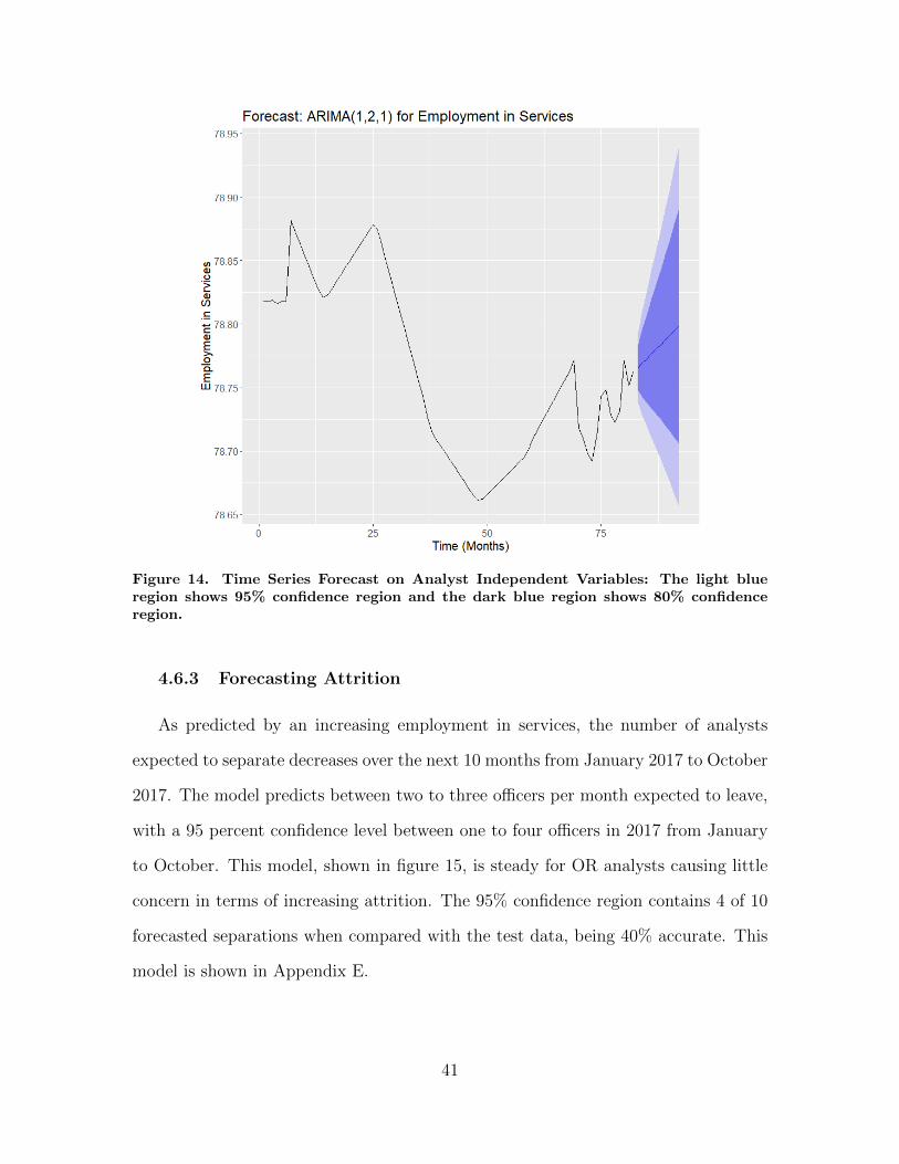
Figure 14. Time Series Forecast on Analyst Independent Variables: The light blueregion shows 95% confidence region and the dark blue region shows 80% confidenceregion.
4.6.3 Forecasting Attrition
As predicted by an increasing employment in services, the number of analysts
expected to separate decreases over the next 10 months from January 2017 to October
2017. The model predicts between two to three officers per month expected to leave,
with a 95 percent confidence level between one to four officers in 2017 from January
to October. This model, shown in figure 15, is steady for OR analysts causing little
concern in terms of increasing attrition. The 95% confidence region contains 4 of 10
forecasted separations when compared with the test data, being 40% accurate. This
model is shown in Appendix E.
41
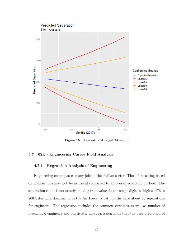
Figure 15. Forecast of Analyst Attrition
4.7 62E - Engineering Career Field Analysis
4.7.1 Regression Analysis of Engineering
Engineering encompasses many jobs in the civilian sector. Thus, forecasting based
on civilian jobs may not be as useful compared to an overall economic outlook. The
separation count is not steady, moving from values in the single digits as high as 178 in
2007, during a downsizing in the Air Force. Most months have about 30 separations
for engineers. The regression includes the common variables as well as number of
mechanical engineers and physicists. The regression finds that the best prediction of
42
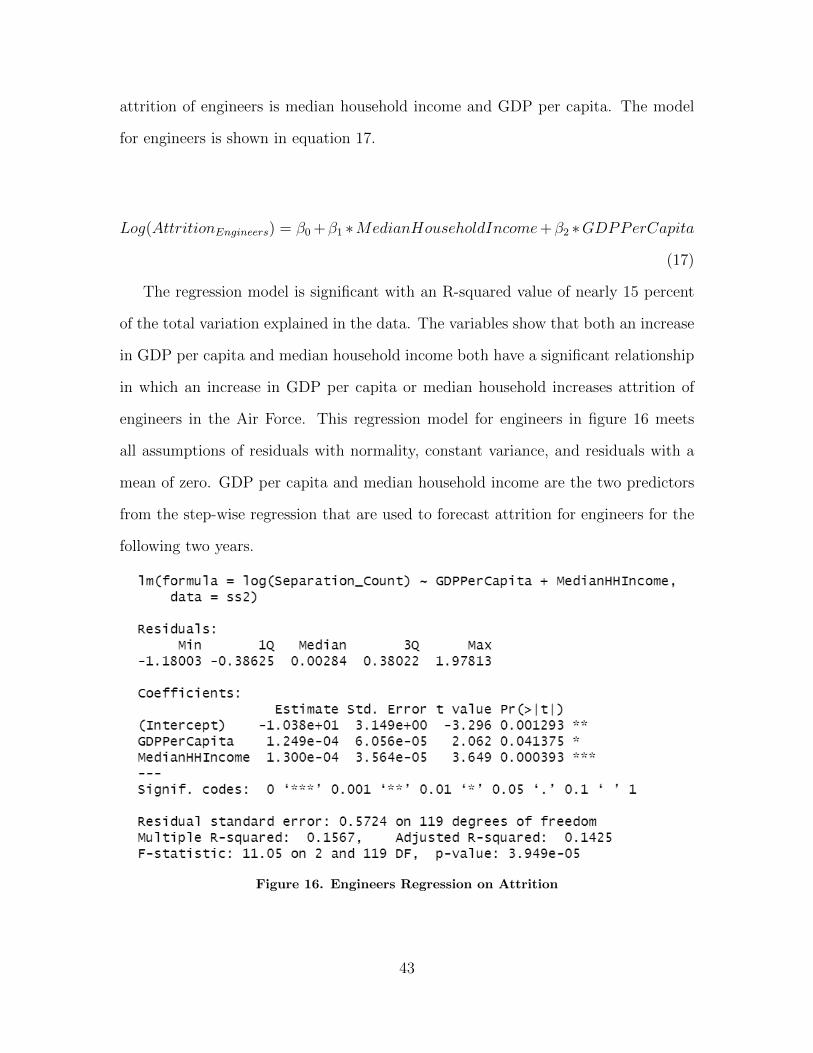
attrition of engineers is median household income and GDP per capita. The model
for engineers is shown in equation 17.
Log(AttritionEngineers) = β0 +β1 ∗MedianHouseholdIncome+β2 ∗GDPPerCapita
(17)
The regression model is significant with an R-squared value of nearly 15 percent
of the total variation explained in the data. The variables show that both an increase
in GDP per capita and median household income both have a significant relationship
in which an increase in GDP per capita or median household increases attrition of
engineers in the Air Force. This regression model for engineers in figure 16 meets
all assumptions of residuals with normality, constant variance, and residuals with a
mean of zero. GDP per capita and median household income are the two predictors
from the step-wise regression that are used to forecast attrition for engineers for the
following two years.
Figure 16. Engineers Regression on Attrition
43
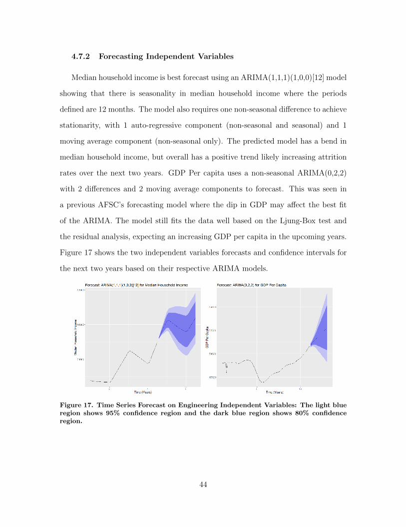
4.7.2 Forecasting Independent Variables
Median household income is best forecast using an ARIMA(1,1,1)(1,0,0)[12] model
showing that there is seasonality in median household income where the periods
defined are 12 months. The model also requires one non-seasonal difference to achieve
stationarity, with 1 auto-regressive component (non-seasonal and seasonal) and 1
moving average component (non-seasonal only). The predicted model has a bend in
median household income, but overall has a positive trend likely increasing attrition
rates over the next two years. GDP Per capita uses a non-seasonal ARIMA(0,2,2)
with 2 differences and 2 moving average components to forecast. This was seen in
a previous AFSC’s forecasting model where the dip in GDP may affect the best fit
of the ARIMA. The model still fits the data well based on the Ljung-Box test and
the residual analysis, expecting an increasing GDP per capita in the upcoming years.
Figure 17 shows the two independent variables forecasts and confidence intervals for
the next two years based on their respective ARIMA models.
Figure 17. Time Series Forecast on Engineering Independent Variables: The light blueregion shows 95% confidence region and the dark blue region shows 80% confidenceregion.
44
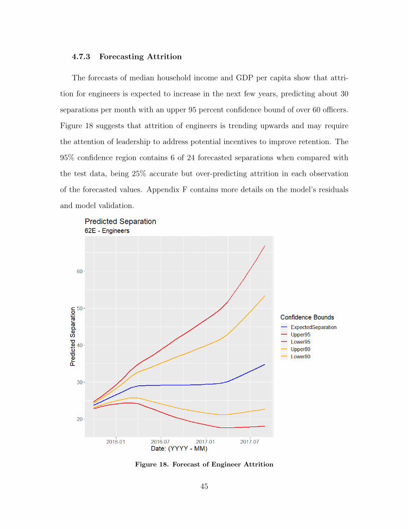
4.7.3 Forecasting Attrition
The forecasts of median household income and GDP per capita show that attri-
tion for engineers is expected to increase in the next few years, predicting about 30
separations per month with an upper 95 percent confidence bound of over 60 officers.
Figure 18 suggests that attrition of engineers is trending upwards and may require
the attention of leadership to address potential incentives to improve retention. The
95% confidence region contains 6 of 24 forecasted separations when compared with
the test data, being 25% accurate but over-predicting attrition in each observation
of the forecasted values. Appendix F contains more details on the model’s residuals
and model validation.
Figure 18. Forecast of Engineer Attrition
45
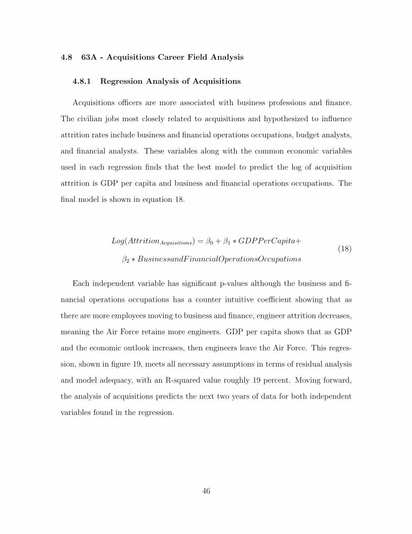
4.8 63A - Acquisitions Career Field Analysis
4.8.1 Regression Analysis of Acquisitions
Acquisitions officers are more associated with business professions and finance.
The civilian jobs most closely related to acquisitions and hypothesized to influence
attrition rates include business and financial operations occupations, budget analysts,
and financial analysts. These variables along with the common economic variables
used in each regression finds that the best model to predict the log of acquisition
attrition is GDP per capita and business and financial operations occupations. The
final model is shown in equation 18.
Log(AttritionAcquisitions) = β0 + β1 ∗GDPPerCapita+
β2 ∗BusinessandF inancialOperationsOccupations(18)
Each independent variable has significant p-values although the business and fi-
nancial operations occupations has a counter intuitive coefficient showing that as
there are more employees moving to business and finance, engineer attrition decreases,
meaning the Air Force retains more engineers. GDP per capita shows that as GDP
and the economic outlook increases, then engineers leave the Air Force. This regres-
sion, shown in figure 19, meets all necessary assumptions in terms of residual analysis
and model adequacy, with an R-squared value roughly 19 percent. Moving forward,
the analysis of acquisitions predicts the next two years of data for both independent
variables found in the regression.
46
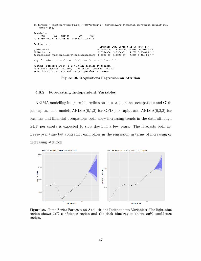
Figure 19. Acquisitions Regression on Attrition
4.8.2 Forecasting Independent Variables
ARIMA modelling in figure 20 predicts business and finance occupations and GDP
per capita. The models ARIMA(0,1,2) for GPD per capita and ARIMA(0,2,2) for
business and financial occupations both show increasing trends in the data although
GDP per capita is expected to slow down in a few years. The forecasts both in-
crease over time but contradict each other in the regression in terms of increasing or
decreasing attrition.
Figure 20. Time Series Forecast on Acquisitions Independent Variables: The light blueregion shows 95% confidence region and the dark blue region shows 80% confidenceregion.
47
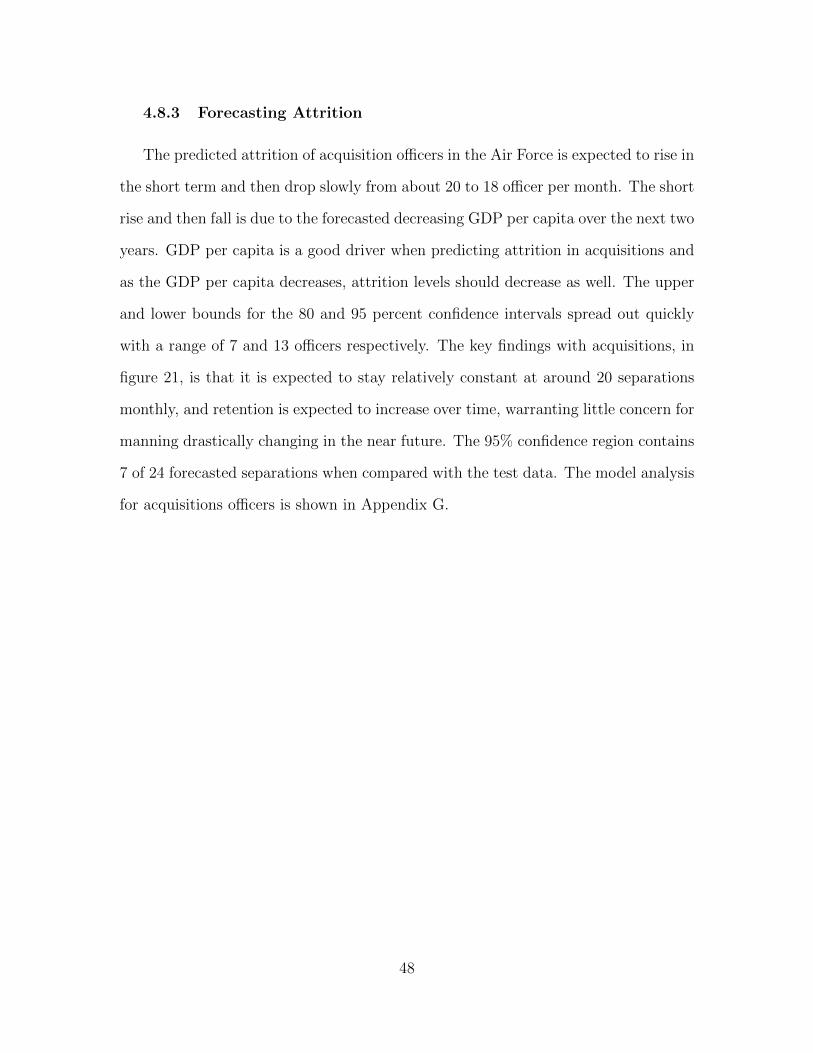
4.8.3 Forecasting Attrition
The predicted attrition of acquisition officers in the Air Force is expected to rise in
the short term and then drop slowly from about 20 to 18 officer per month. The short
rise and then fall is due to the forecasted decreasing GDP per capita over the next two
years. GDP per capita is a good driver when predicting attrition in acquisitions and
as the GDP per capita decreases, attrition levels should decrease as well. The upper
and lower bounds for the 80 and 95 percent confidence intervals spread out quickly
with a range of 7 and 13 officers respectively. The key findings with acquisitions, in
figure 21, is that it is expected to stay relatively constant at around 20 separations
monthly, and retention is expected to increase over time, warranting little concern for
manning drastically changing in the near future. The 95% confidence region contains
7 of 24 forecasted separations when compared with the test data. The model analysis
for acquisitions officers is shown in Appendix G.
48
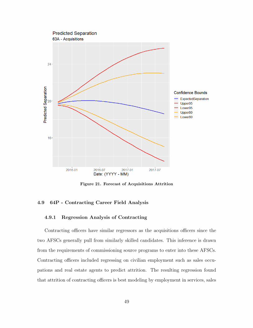
Figure 21. Forecast of Acquisitions Attrition
4.9 64P - Contracting Career Field Analysis
4.9.1 Regression Analysis of Contracting
Contracting officers have similar regressors as the acquisitions officers since the
two AFSCs generally pull from similarly skilled candidates. This inference is drawn
from the requirements of commissioning source programs to enter into these AFSCs.
Contracting officers included regressing on civilian employment such as sales occu-
pations and real estate agents to predict attrition. The resulting regression found
that attrition of contracting officers is best modeling by employment in services, sales
49
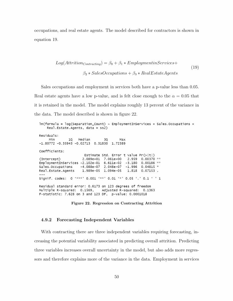
occupations, and real estate agents. The model described for contractors is shown in
equation 19.
Log(AttritionContracting) = β0 + β1 ∗ EmploymentinServices+
β2 ∗ SalesOccupations+ β3 ∗RealEstateAgents(19)
Sales occupations and employment in services both have a p-value less than 0.05.
Real estate agents have a low p-value, and is felt close enough to the α = 0.05 that
it is retained in the model. The model explains roughly 13 percent of the variance in
the data. The model described is shown in figure 22.
Figure 22. Regression on Contracting Attrition
4.9.2 Forecasting Independent Variables
With contracting there are three independent variables requiring forecasting, in-
creasing the potential variability associated in predicting overall attrition. Predicting
three variables increases overall uncertainty in the model, but also adds more regres-
sors and therefore explains more of the variance in the data. Employment in services
50

is best fit using ARIMA(0,1,2), sales occupation using ARIMA(1,2,1), and real estate
agents with ARIMA(2,2,0). The ARIMA models for each of the three independent
variables described are shown in figure 23. Slight increases in employment in services
and sales occupations are expected with almost no change expected for real estate
agents by the Box-Jenkins (ARIMA) models. The combination of all three forecasts
affects predicted attrition of contracting officers for the next 12 months. The forecasts
are curtailed by one year because of the recession in 2008 and the observations during
and the recession are removed as outliers. ARIMA modelling requires continuity, so
the observations prior to the recession are also removed to satisfy the assumptions
of the model. The forecasts following removal of observations cover one year beyond
the last observation in March 2016.
51
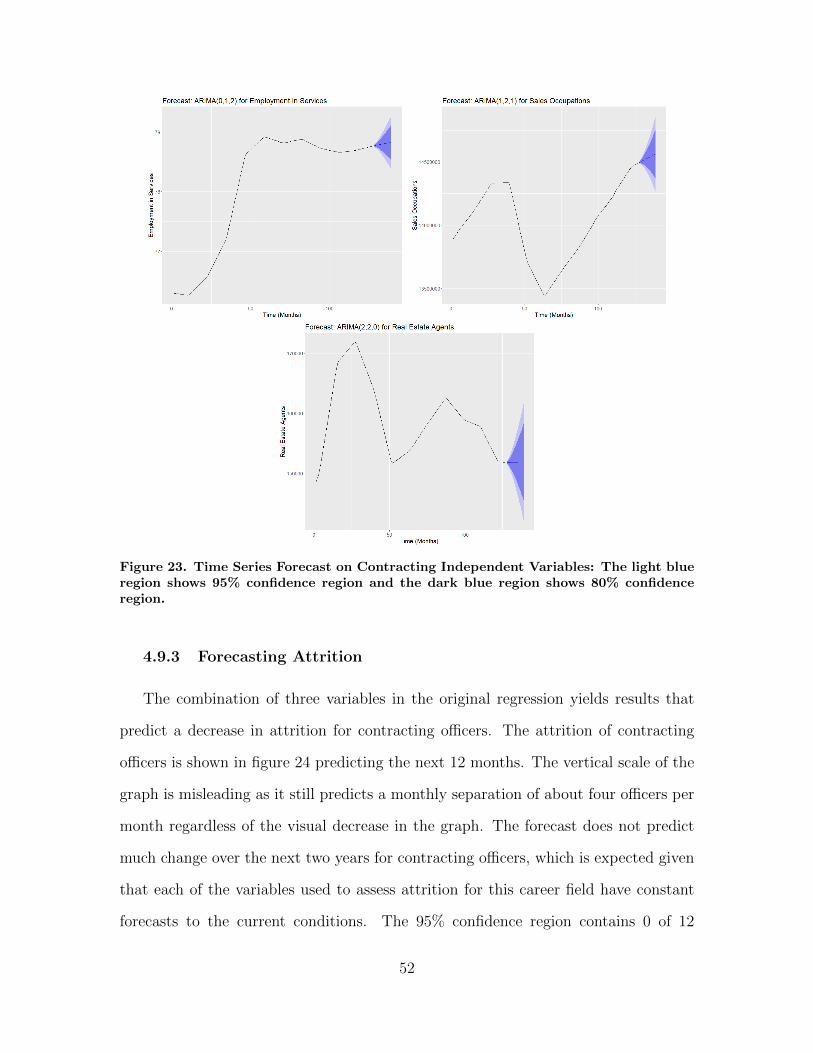
Figure 23. Time Series Forecast on Contracting Independent Variables: The light blueregion shows 95% confidence region and the dark blue region shows 80% confidenceregion.
4.9.3 Forecasting Attrition
The combination of three variables in the original regression yields results that
predict a decrease in attrition for contracting officers. The attrition of contracting
officers is shown in figure 24 predicting the next 12 months. The vertical scale of the
graph is misleading as it still predicts a monthly separation of about four officers per
month regardless of the visual decrease in the graph. The forecast does not predict
much change over the next two years for contracting officers, which is expected given
that each of the variables used to assess attrition for this career field have constant
forecasts to the current conditions. The 95% confidence region contains 0 of 12
52
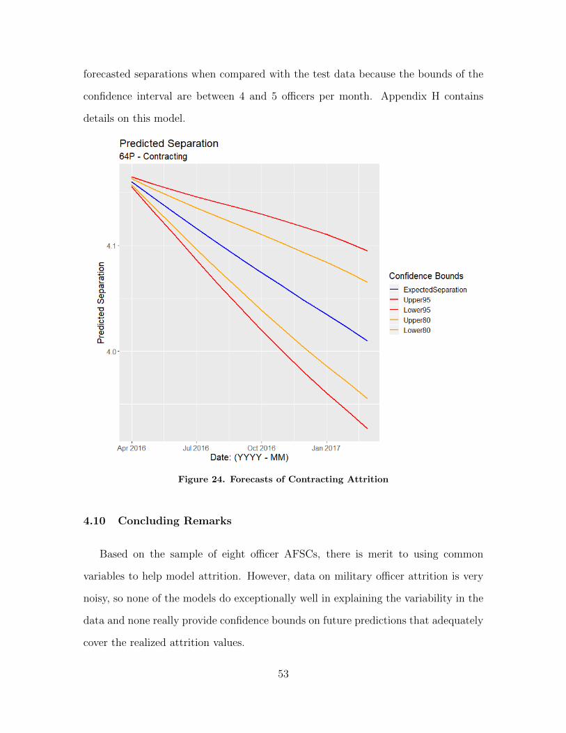
forecasted separations when compared with the test data because the bounds of the
confidence interval are between 4 and 5 officers per month. Appendix H contains
details on this model.
Figure 24. Forecasts of Contracting Attrition
4.10 Concluding Remarks
Based on the sample of eight officer AFSCs, there is merit to using common
variables to help model attrition. However, data on military officer attrition is very
noisy, so none of the models do exceptionally well in explaining the variability in the
data and none really provide confidence bounds on future predictions that adequately
cover the realized attrition values.
53
V. Conclusions and Future Research
5.1 Review
The United States Air Force has a complex system for recruiting and promotion,
which needs to retain current talent to properly function. Understanding the factors
that may cause attrition levels to increase, and predicting future attrition levels will
inform leadership of at-risk AFSCs in terms of manning. Additionally, predicting
influxes in attrition will help recruiting and assessing incentive programs for career
fields. Gaining relevant information to the retention problem by AFSC will create a
more stable and capable U.S. Air Force.
5.2 Results
The results from the analysis show that AFSCs have a relationship with compara-
ble jobs in the civilian sector. Seven of the eight AFSCs in the study show significant
results when using civilian employment to predict attrition. Only one, 62E (Engi-
neers), were more receptive to overall economic conditions as the influential factors.
We also find that attrition in the Air Force does not increase or decrease uniformly
by AFSC, but rather individually, suggesting models be tailored specifically to the
AFSC in order to best predict attrition. Table 3 shows the consolidated results of
each AFSC, showing the overall trend of the AFSC’s attrition, the expected monthly
attrition rate currently, a year from now, and two years from now. The percentage
is measured by the monthly attrition divided by the number assigned to the AFSC.
This shows the monthly percentage expected to separate from the Air Force. OR
analysts and contractors have an NA two years from now to show that the forecasts
are not made available due to insufficient data.
54
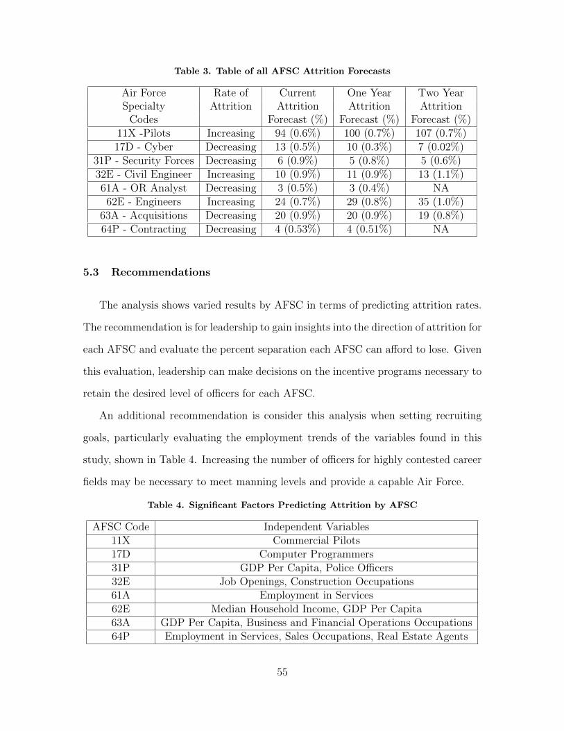
Table 3. Table of all AFSC Attrition Forecasts
Air Force Rate of Current One Year Two YearSpecialty Attrition Attrition Attrition Attrition
Codes Forecast (%) Forecast (%) Forecast (%)11X -Pilots Increasing 94 (0.6%) 100 (0.7%) 107 (0.7%)17D - Cyber Decreasing 13 (0.5%) 10 (0.3%) 7 (0.02%)
31P - Security Forces Decreasing 6 (0.9%) 5 (0.8%) 5 (0.6%)32E - Civil Engineer Increasing 10 (0.9%) 11 (0.9%) 13 (1.1%)61A - OR Analyst Decreasing 3 (0.5%) 3 (0.4%) NA62E - Engineers Increasing 24 (0.7%) 29 (0.8%) 35 (1.0%)
63A - Acquisitions Decreasing 20 (0.9%) 20 (0.9%) 19 (0.8%)64P - Contracting Decreasing 4 (0.53%) 4 (0.51%) NA
5.3 Recommendations
The analysis shows varied results by AFSC in terms of predicting attrition rates.
The recommendation is for leadership to gain insights into the direction of attrition for
each AFSC and evaluate the percent separation each AFSC can afford to lose. Given
this evaluation, leadership can make decisions on the incentive programs necessary to
retain the desired level of officers for each AFSC.
An additional recommendation is consider this analysis when setting recruiting
goals, particularly evaluating the employment trends of the variables found in this
study, shown in Table 4. Increasing the number of officers for highly contested career
fields may be necessary to meet manning levels and provide a capable Air Force.
Table 4. Significant Factors Predicting Attrition by AFSC
AFSC Code Independent Variables11X Commercial Pilots17D Computer Programmers31P GDP Per Capita, Police Officers32E Job Openings, Construction Occupations61A Employment in Services62E Median Household Income, GDP Per Capita63A GDP Per Capita, Business and Financial Operations Occupations64P Employment in Services, Sales Occupations, Real Estate Agents
55
5.4 Future Research
Forecasting human behavior is difficult. Humans are irrational beings and highly
unpredictable, but correlations between attrition and common data do exist and there
is more data to provide greater forecasts. A key indicator for predicting attrition
is years of service and the demographics associated with an individual. Prior to
forecasting attrition levels based on economic conditions the individual officer could
be studied to determine the likelihood of separation. The economic conditions should
be considered an afterthought, following a logistic regression to predict individual
separation. There is difficulty obtaining the personally identifiable information data
and having access to analyze each individual on a big data scale.
Predicting individual retention is necessary, but more economic factors can easily
be obtained to predict attrition. The quality of data is more questionable than the ac-
cess of economic data. Most of the data gathered in this analysis was either quarterly
or biannual, causing problems predicting monthly data. Aggregating the number of
separations monthly to annually may be more accurate in predicting attrition levels.
Monthly attrition rates have large variation, and a single estimate of highly variable
data is not useful. The confidence intervals associated with the forecasts are also not
the most accurate predictions of the data, which likely stems from low R-squared
values in the regressions. Aggregating the monthly separations, finding more em-
ployment factors for regression, and ensuring better quality data could be better for
predictive purposes and used to extend this research.
Overall attrition can be better modelled by combining the prediction of individual
attrition and introducing more regressors to the model to increase the R2 values for
each regression. This would increase predictive accuracy for attrition, but under-
standing manning in a career field is dependent on recruitment as well. Incorporating
a growth of recruitment model may prove beneficial to achieve desired manning levels
56

for each AFSC and retain capable officers in the Air Force.
57
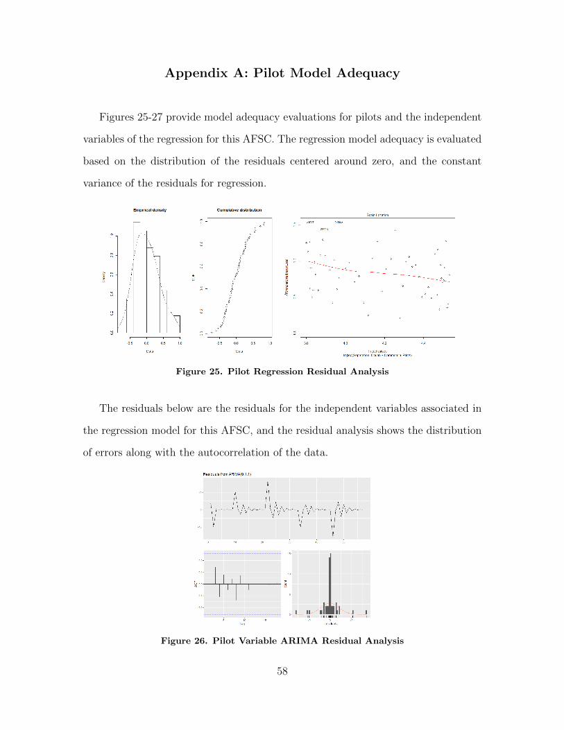
Appendix A: Pilot Model Adequacy
Figures 25-27 provide model adequacy evaluations for pilots and the independent
variables of the regression for this AFSC. The regression model adequacy is evaluated
based on the distribution of the residuals centered around zero, and the constant
variance of the residuals for regression.
Figure 25. Pilot Regression Residual Analysis
The residuals below are the residuals for the independent variables associated in
the regression model for this AFSC, and the residual analysis shows the distribution
of errors along with the autocorrelation of the data.
Figure 26. Pilot Variable ARIMA Residual Analysis
58
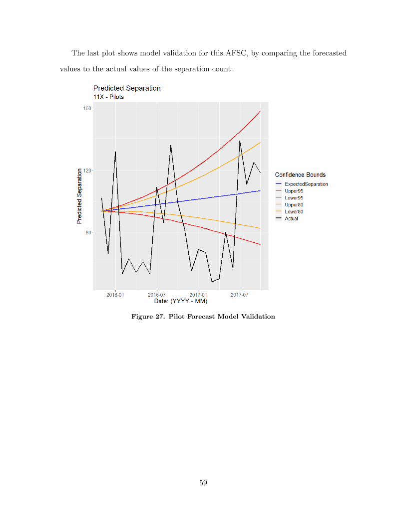
The last plot shows model validation for this AFSC, by comparing the forecasted
values to the actual values of the separation count.
Figure 27. Pilot Forecast Model Validation
59
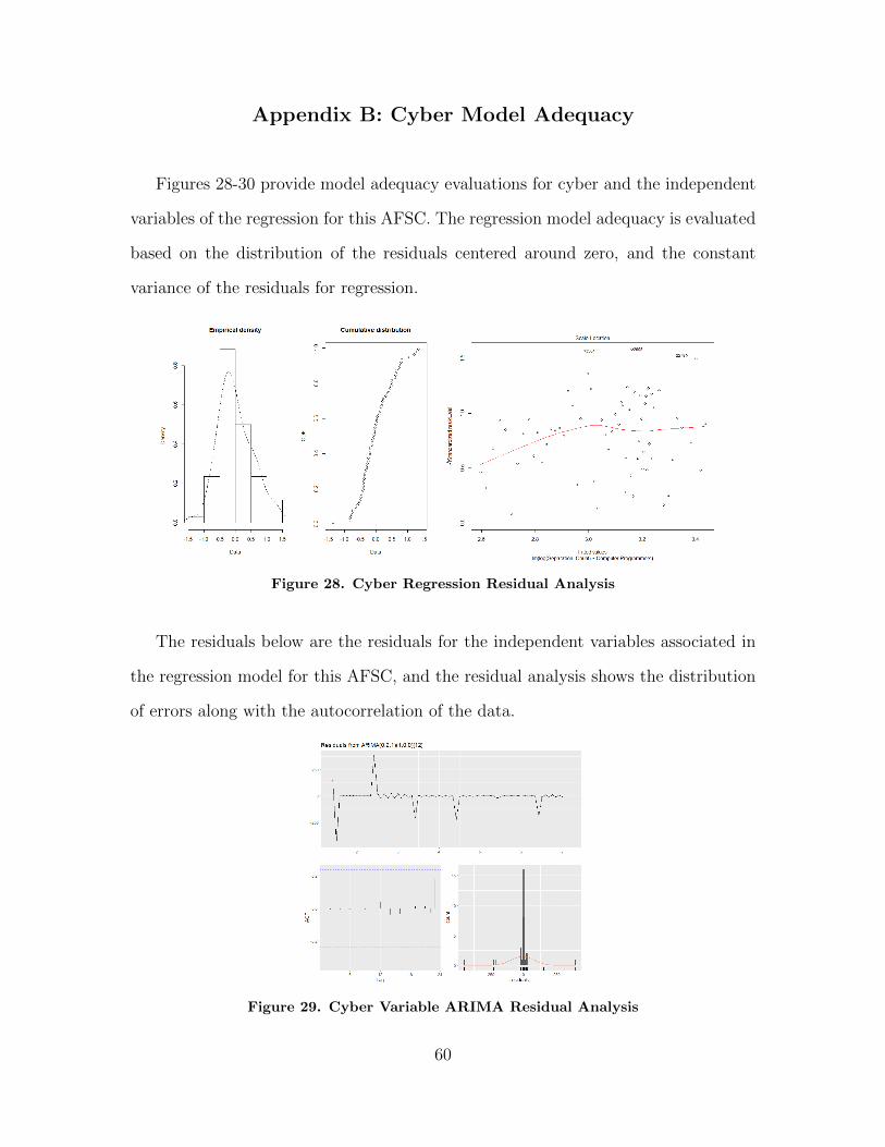
Appendix B: Cyber Model Adequacy
Figures 28-30 provide model adequacy evaluations for cyber and the independent
variables of the regression for this AFSC. The regression model adequacy is evaluated
based on the distribution of the residuals centered around zero, and the constant
variance of the residuals for regression.
Figure 28. Cyber Regression Residual Analysis
The residuals below are the residuals for the independent variables associated in
the regression model for this AFSC, and the residual analysis shows the distribution
of errors along with the autocorrelation of the data.
Figure 29. Cyber Variable ARIMA Residual Analysis
60
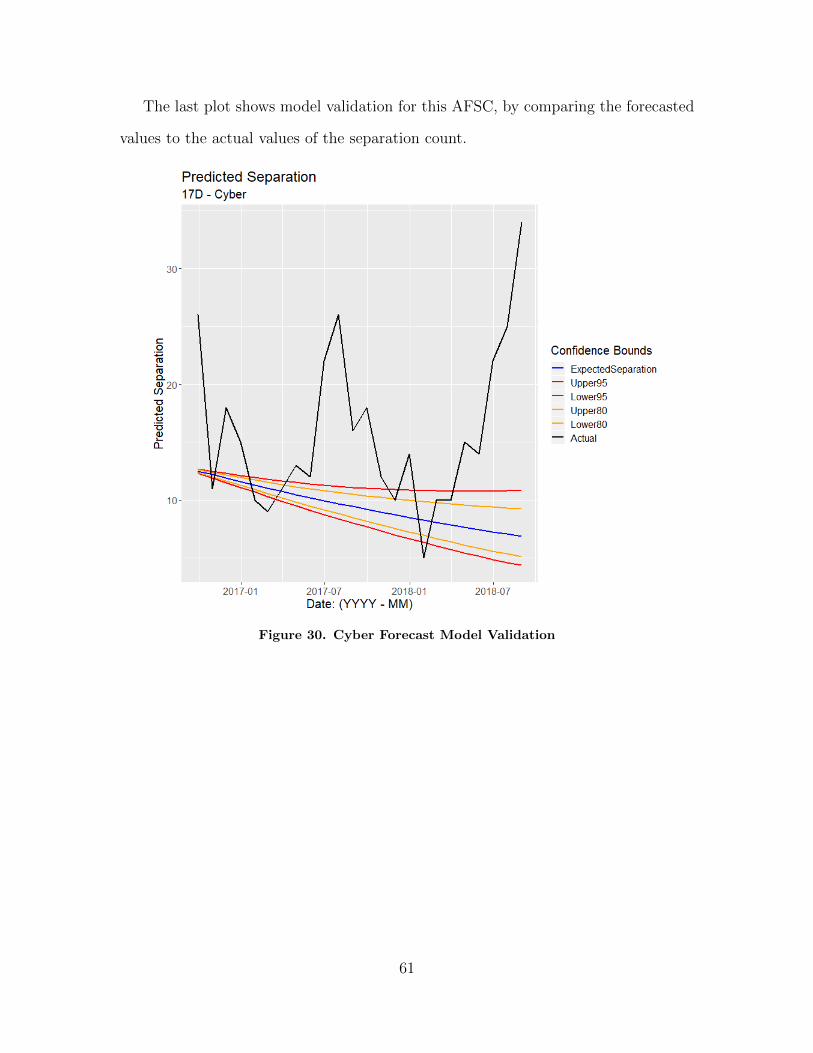
The last plot shows model validation for this AFSC, by comparing the forecasted
values to the actual values of the separation count.
Figure 30. Cyber Forecast Model Validation
61
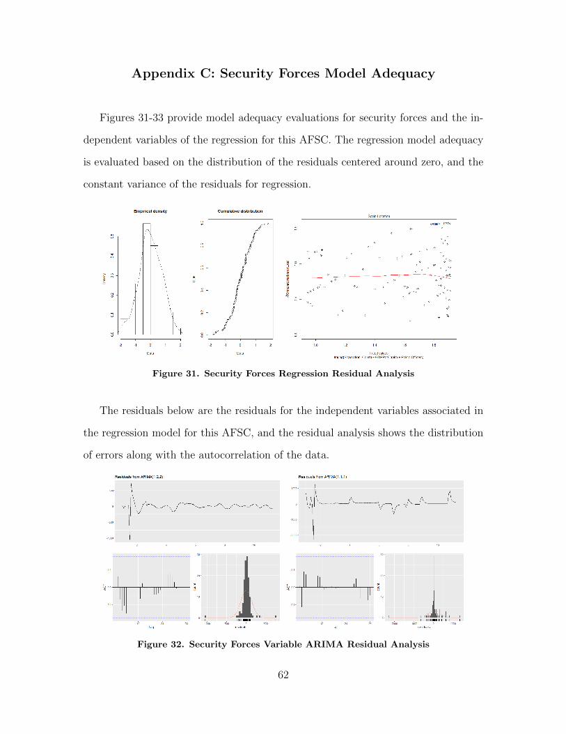
Appendix C: Security Forces Model Adequacy
Figures 31-33 provide model adequacy evaluations for security forces and the in-
dependent variables of the regression for this AFSC. The regression model adequacy
is evaluated based on the distribution of the residuals centered around zero, and the
constant variance of the residuals for regression.
Figure 31. Security Forces Regression Residual Analysis
The residuals below are the residuals for the independent variables associated in
the regression model for this AFSC, and the residual analysis shows the distribution
of errors along with the autocorrelation of the data.
Figure 32. Security Forces Variable ARIMA Residual Analysis
62
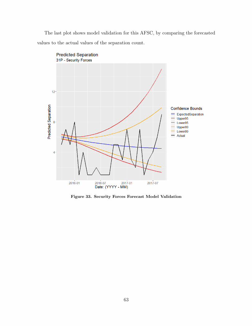
The last plot shows model validation for this AFSC, by comparing the forecasted
values to the actual values of the separation count.
Figure 33. Security Forces Forecast Model Validation
63
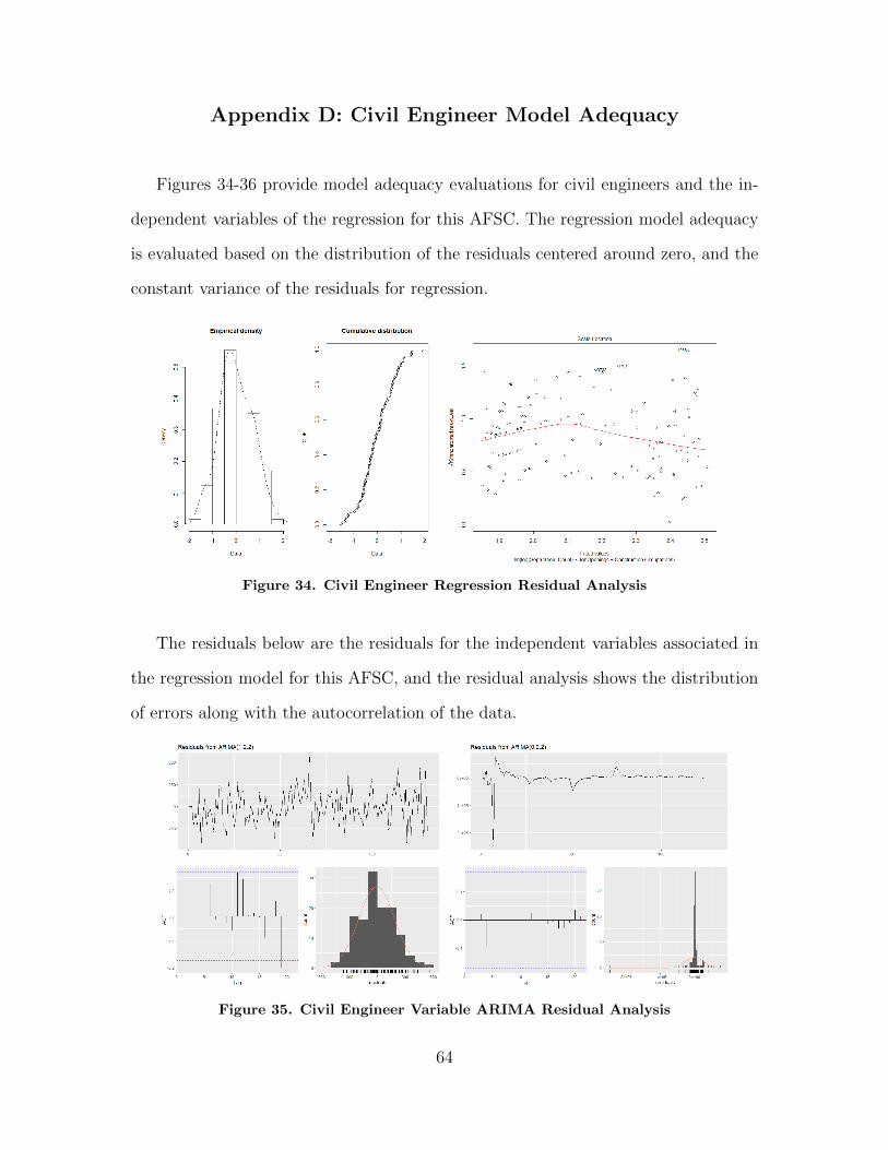
Appendix D: Civil Engineer Model Adequacy
Figures 34-36 provide model adequacy evaluations for civil engineers and the in-
dependent variables of the regression for this AFSC. The regression model adequacy
is evaluated based on the distribution of the residuals centered around zero, and the
constant variance of the residuals for regression.
Figure 34. Civil Engineer Regression Residual Analysis
The residuals below are the residuals for the independent variables associated in
the regression model for this AFSC, and the residual analysis shows the distribution
of errors along with the autocorrelation of the data.
Figure 35. Civil Engineer Variable ARIMA Residual Analysis
64
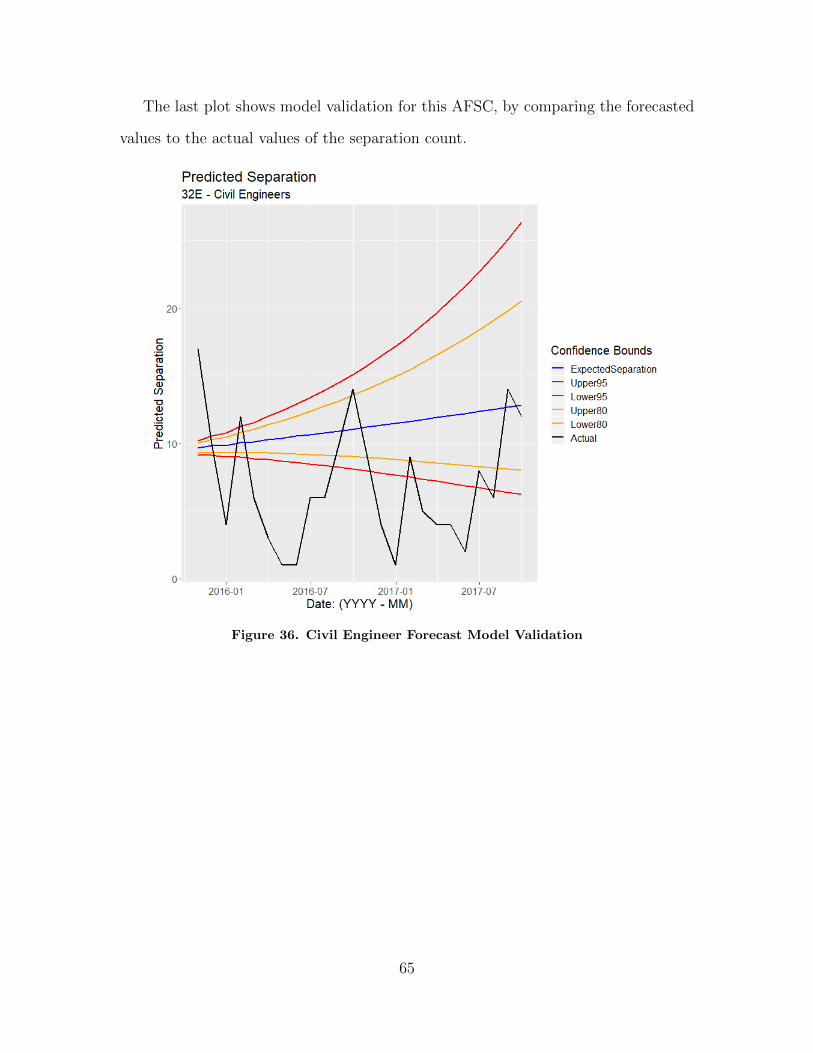
The last plot shows model validation for this AFSC, by comparing the forecasted
values to the actual values of the separation count.
Figure 36. Civil Engineer Forecast Model Validation
65
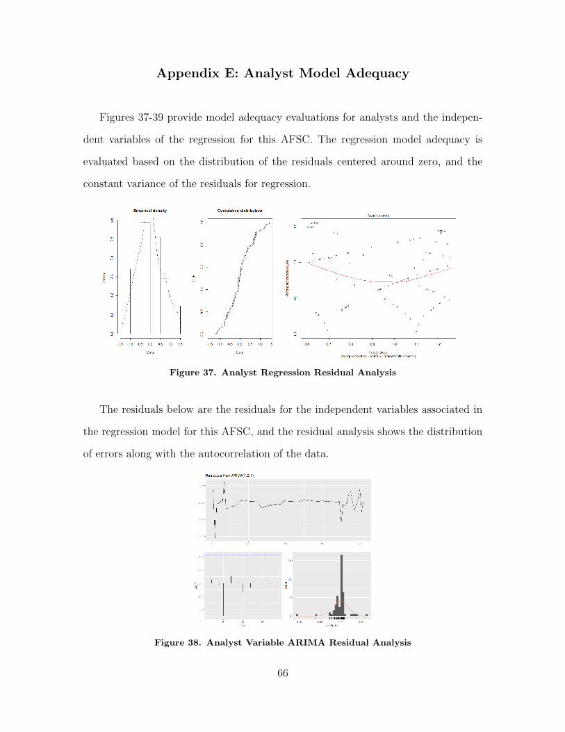
Appendix E: Analyst Model Adequacy
Figures 37-39 provide model adequacy evaluations for analysts and the indepen-
dent variables of the regression for this AFSC. The regression model adequacy is
evaluated based on the distribution of the residuals centered around zero, and the
constant variance of the residuals for regression.
Figure 37. Analyst Regression Residual Analysis
The residuals below are the residuals for the independent variables associated in
the regression model for this AFSC, and the residual analysis shows the distribution
of errors along with the autocorrelation of the data.
Figure 38. Analyst Variable ARIMA Residual Analysis
66
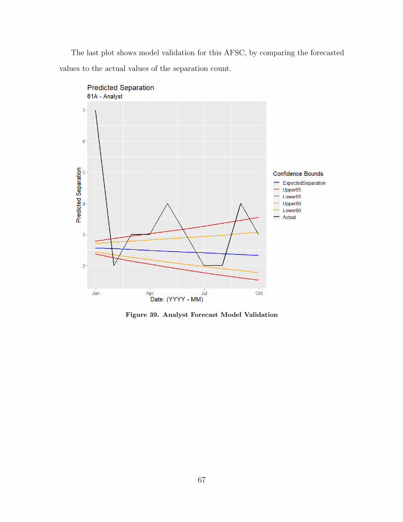
The last plot shows model validation for this AFSC, by comparing the forecasted
values to the actual values of the separation count.
Figure 39. Analyst Forecast Model Validation
67
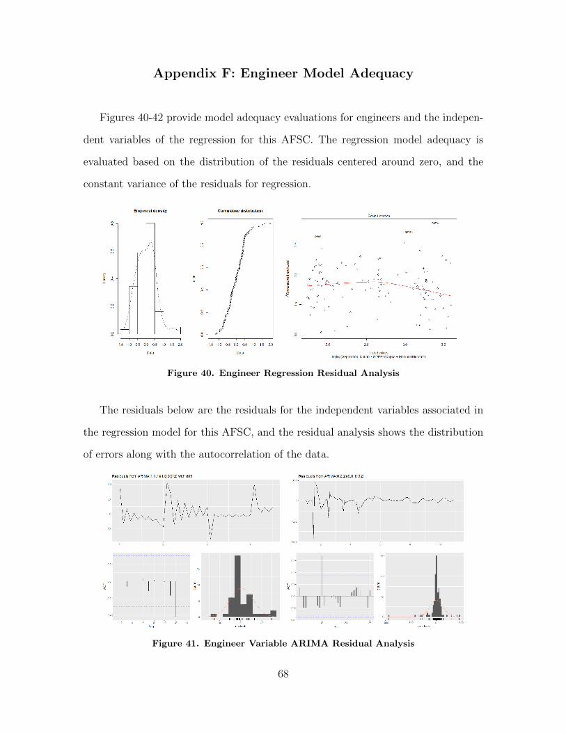
Appendix F: Engineer Model Adequacy
Figures 40-42 provide model adequacy evaluations for engineers and the indepen-
dent variables of the regression for this AFSC. The regression model adequacy is
evaluated based on the distribution of the residuals centered around zero, and the
constant variance of the residuals for regression.
Figure 40. Engineer Regression Residual Analysis
The residuals below are the residuals for the independent variables associated in
the regression model for this AFSC, and the residual analysis shows the distribution
of errors along with the autocorrelation of the data.
Figure 41. Engineer Variable ARIMA Residual Analysis
68
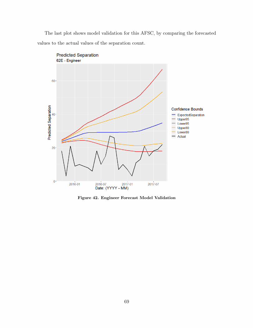
The last plot shows model validation for this AFSC, by comparing the forecasted
values to the actual values of the separation count.
Figure 42. Engineer Forecast Model Validation
69
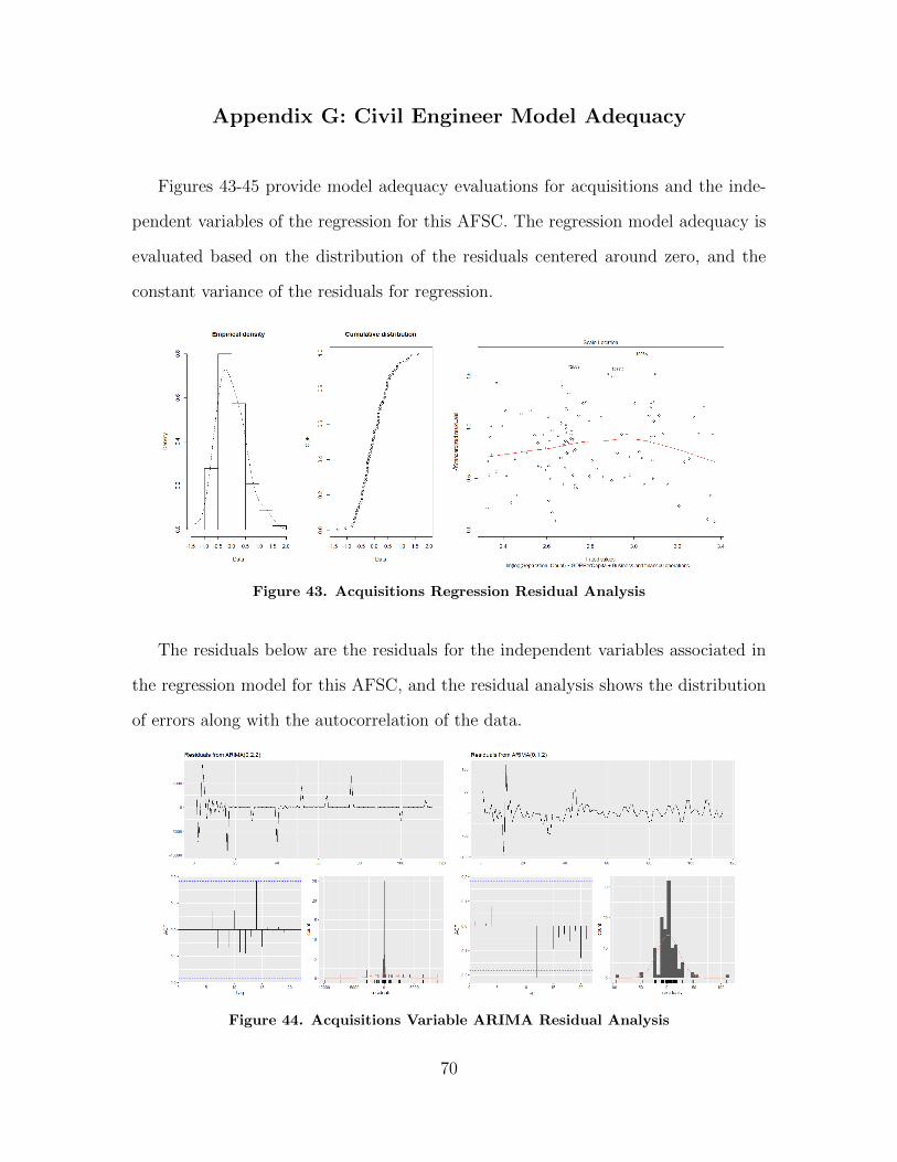
Appendix G: Civil Engineer Model Adequacy
Figures 43-45 provide model adequacy evaluations for acquisitions and the inde-
pendent variables of the regression for this AFSC. The regression model adequacy is
evaluated based on the distribution of the residuals centered around zero, and the
constant variance of the residuals for regression.
Figure 43. Acquisitions Regression Residual Analysis
The residuals below are the residuals for the independent variables associated in
the regression model for this AFSC, and the residual analysis shows the distribution
of errors along with the autocorrelation of the data.
Figure 44. Acquisitions Variable ARIMA Residual Analysis
70
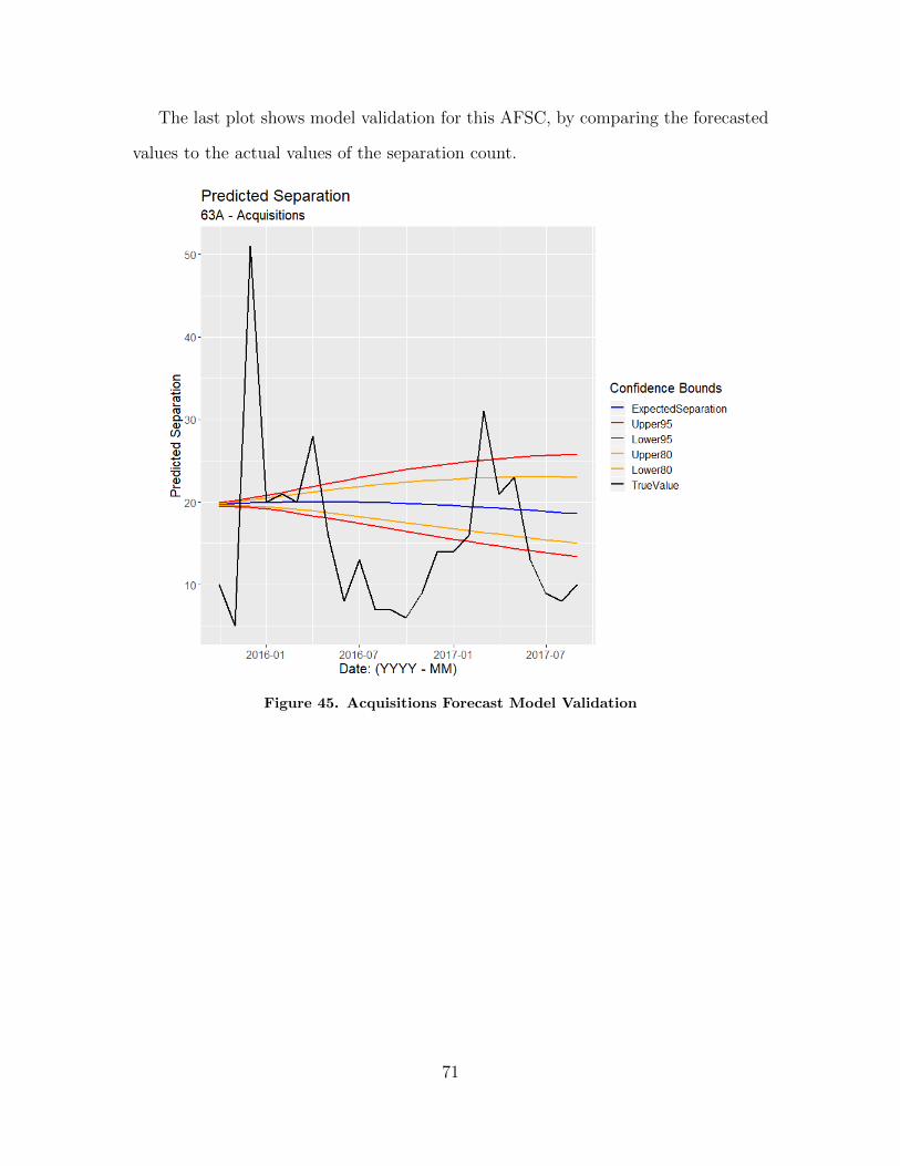
The last plot shows model validation for this AFSC, by comparing the forecasted
values to the actual values of the separation count.
Figure 45. Acquisitions Forecast Model Validation
71
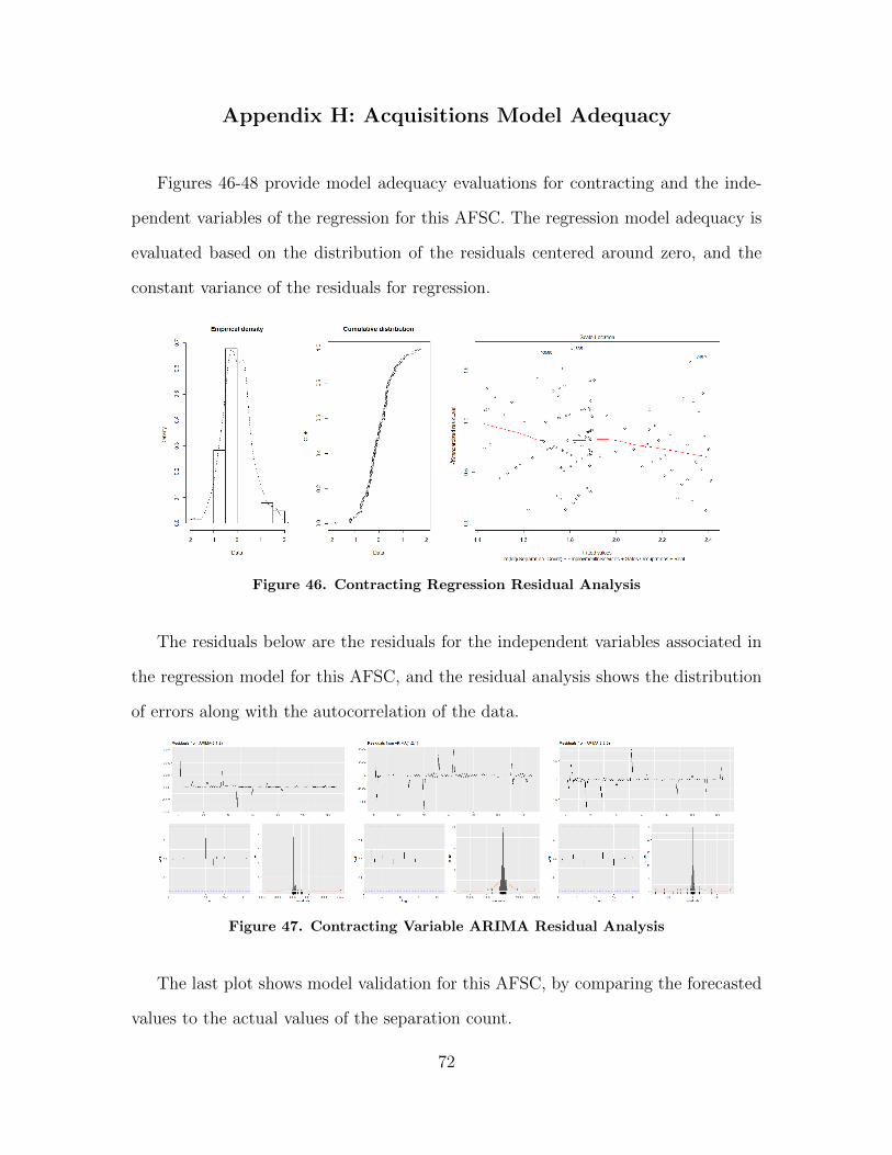
Appendix H: Acquisitions Model Adequacy
Figures 46-48 provide model adequacy evaluations for contracting and the inde-
pendent variables of the regression for this AFSC. The regression model adequacy is
evaluated based on the distribution of the residuals centered around zero, and the
constant variance of the residuals for regression.
Figure 46. Contracting Regression Residual Analysis
The residuals below are the residuals for the independent variables associated in
the regression model for this AFSC, and the residual analysis shows the distribution
of errors along with the autocorrelation of the data.
Figure 47. Contracting Variable ARIMA Residual Analysis
The last plot shows model validation for this AFSC, by comparing the forecasted
values to the actual values of the separation count.
72
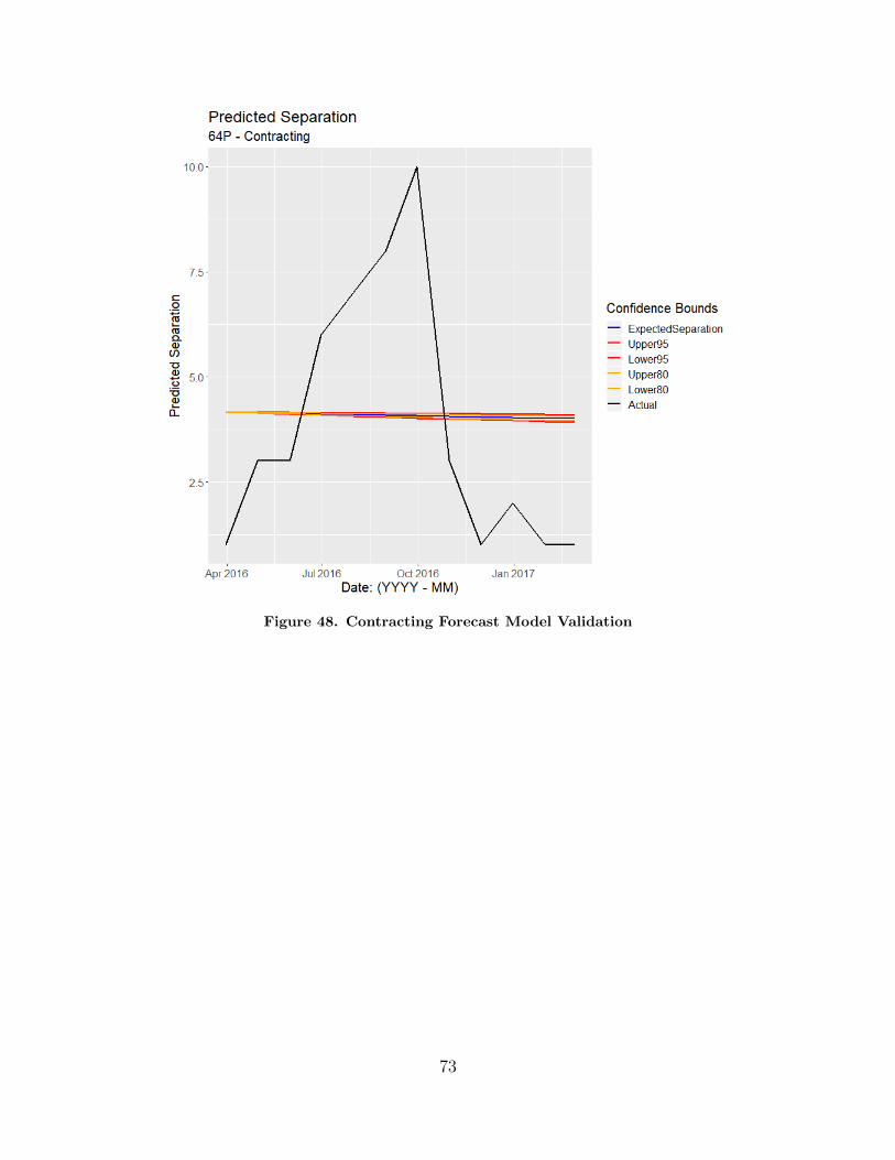
Figure 48. Contracting Forecast Model Validation
73
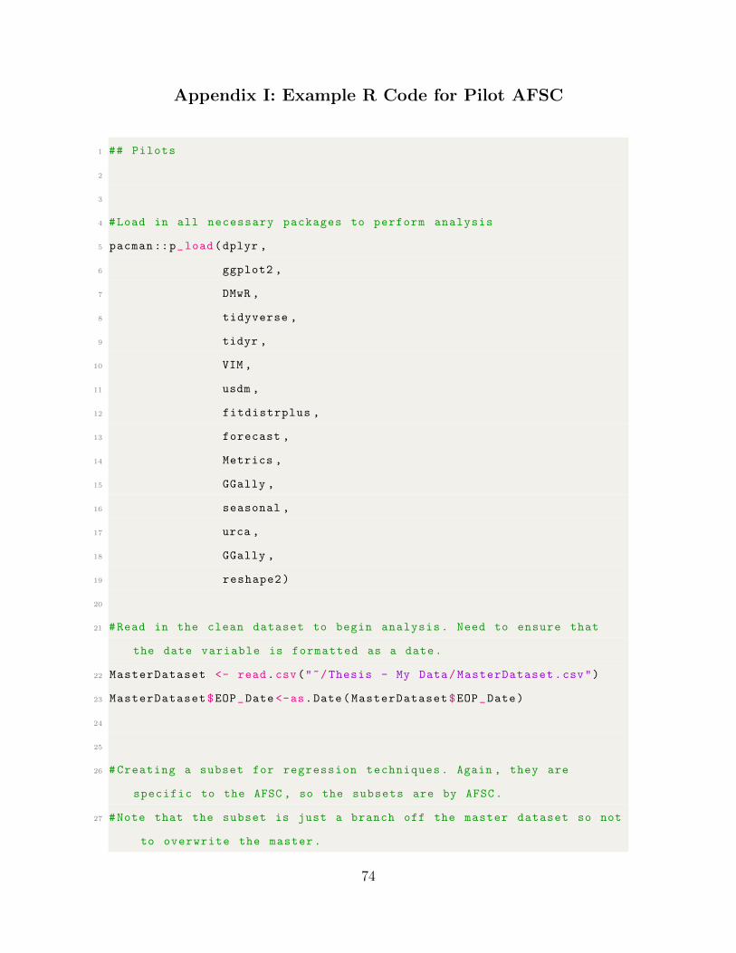
Appendix I: Example R Code for Pilot AFSC
1 ## Pilots
2
3
4 #Load in all necessary packages to perform analysis
5 pacman ::p_load(dplyr ,
6 ggplot2 ,
7 DMwR ,
8 tidyverse ,
9 tidyr ,
10 VIM ,
11 usdm ,
12 fitdistrplus ,
13 forecast ,
14 Metrics ,
15 GGally ,
16 seasonal ,
17 urca ,
18 GGally ,
19 reshape2)
20
21 #Read in the clean dataset to begin analysis. Need to ensure that
the date variable is formatted as a date.
22 MasterDataset <- read.csv("~/Thesis - My Data/MasterDataset.csv")
23 MasterDataset$EOP_Date <-as.Date(MasterDataset$EOP_Date)
24
25
26 #Creating a subset for regression techniques. Again , they are
specific to the AFSC , so the subsets are by AFSC.
27 #Note that the subset is just a branch off the master dataset so not
to overwrite the master.
74
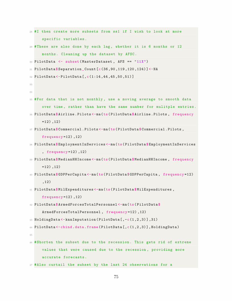
28 #I then create more subsets from ss1 if I wish to look at more
specific variables.
29 #These are also done by each lag , whether it is 6 months or 12
months. Cleaning up the dataset by AFSC.
30 PilotData <- subset(MasterDataset , AFS == "11X")
31 PilotData$Separation_Count[c(36 ,90 ,119 ,120 ,124)]<-NA
32 PilotData <-PilotData[,c(1:14 ,44 ,45 ,50 ,51)]
33
34
35 #For data that is not monthly , use a moving average to smooth data
over time , rather than have the same number for mulitple entries.
36 PilotData$Airline.Pilots <-ma(ts(PilotData$Airline.Pilots , frequency
=12) ,12)
37 PilotData$Commercial.Pilots <-ma(ts(PilotData$Commercial.Pilots ,
frequency =12) ,12)
38 PilotData$EmploymentInServices <-ma(ts(PilotData$EmploymentInServices
, frequency =12) ,12)
39 PilotData$MedianHHIncome <-ma(ts(PilotData$MedianHHIncome , frequency
=12) ,12)
40 PilotData$GDPPerCapita <-ma(ts(PilotData$GDPPerCapita , frequency =12)
,12)
41 PilotData$MilExpenditures <-ma(ts(PilotData$MilExpenditures ,
frequency =12) ,12)
42 PilotData$ArmedForcesTotalPersonnel <-ma(ts(PilotData$
ArmedForcesTotalPersonnel , frequency =12) ,12)
43 HoldingData <-knnImputation(PilotData[,-c(1,2,3)],31)
44 PilotData <-cbind.data.frame(PilotData[,c(1,2,3)],HoldingData)
45
46 #Shorten the subset due to the recession. This gets rid of extreme
values that were caused due to the recession , providing more
accurate forecasts.
47 #Also curtail the subset by the last 24 observations for a
75
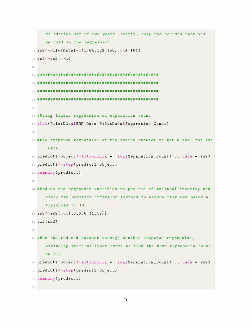
validation set of two years. Lastly , keep the columns that will
be used in the regression.
48 ss2 <-PilotData[-c(1:64 ,122:156) ,c(4:16)]
49 ss2 <-ss2[,-10]
50
51 ###############################################
52 ###############################################
53 ###############################################
54 ###############################################
55
56 #Using linear regression on separation count
57 plot(PilotData$EOP_Date ,PilotData$Separation_Count)
58
59 #Use stepwise regression on the entire dataset to get a feel for the
data.
60 predict1.object <-lm(formula = log(Separation_Count)~., data = ss2)
61 predict1 <-step(predict1.object)
62 summary(predict1)
63
64 #Reduce the regressor variables to get rid of mulitcollinearity and
check teh variance inflation factors to ensure they are below a
threshold of 10.
65 ss2 <-ss2[,c(1,3,5,6,11,12)]
66 vif(ss2)
67
68 #Run the reduced dataset through another stepwise regression ,
excluding multicollinear terms to find the best regression based
on AIC.
69 predict1.object <-lm(formula = log(Separation_Count)~., data = ss2)
70 predict1 <-step(predict1.object)
71 summary(predict1)
72
76
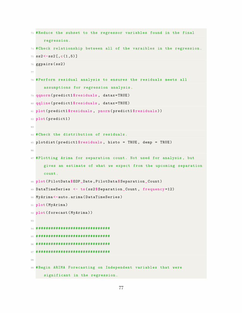
73 #Reduce the subset to the regressor variables found in the final
regression.
74 #Check relationship between all of the varaibles in the regression.
75 ss2 <-ss2[,c(1,5)]
76 ggpairs(ss2)
77
78 #Perform residual analysis to ensures the residuals meets all
assumptions for regression analysis.
79 qqnorm(predict1$residuals , datax=TRUE)
80 qqline(predict1$residuals , datax=TRUE)
81 plot(predict1$residuals , pnorm(predict1$residuals))
82 plot(predict1)
83
84 #Check the distribution of residuals.
85 plotdist(predict1$residuals , histo = TRUE , demp = TRUE)
86
87 #Plotting Arima for separation count. Not used for analysis , but
gives an estimate of what we expect from the upcoming separation
count.
88 plot(PilotData$EOP_Date ,PilotData$Separation_Count)
89 DataTimeSeries <- ts(ss2$Separation_Count , frequency =12)
90 MyArima <-auto.arima(DataTimeSeries)
91 plot(MyArima)
92 plot(forecast(MyArima))
93
94 ##############################
95 ##############################
96 ##############################
97 ##############################
98
99 #Begin ARIMA Forecasting on Independent variables that were
significant in the regression.
77
100 #For pilots we found Commercial.Pilots as the only significant
variable in the regression.
101
102 #Plot the data for commercial pilot employment.
103 plot(PilotData$EOP_Date ,PilotData$Commercial.Pilots)
104
105 #Create a time series vector of the data.
106 DataTimeSeries <- ts(ss2$Commercial.Pilots , frequency =12)
107
108 #Use auto.arima to get a feel for the model needed. Subject to
updates based on the complexity of the model.
109 MyArima <-auto.arima(DataTimeSeries , approximation = FALSE)
110
111 #Plot the roots to ensure all points are within the unti circle.
112 plot(MyArima)
113
114 #Get a visual plot of the ARIMA model.
115 plot(forecast(MyArima))
116
117 #Rerun the arima model to find a balance between predictive accuracy
, resiudal analysis , autocorrelation analysis , and model
complexity.
118 MyArima <-arima(ss2$Commercial.Pilots , order = c(0,1,1), seasonal =
list(order = c(0,1,1)))
119 MyArima
120
121 #Forecast the updated ARIMA model for the next 24 months , with the
default confidence bounds of 95% and 80%.
122 MyForecast <-forecast(MyArima , h=24)
123
124 #Plot the forecast of the data and clean up the axes for better
presenting the data.
78
125 autoplot(MyForecast)+ggtitle("Forecast: ARIMA (0,1,1) for Commercial
Pilots")+xlab("Time (Months)")+ylab("Commercial Pilot Employment"
)+theme(text = element_text(size = 15))
126
127 #Check the residuals of the forecast and model to ensure the model
meets all assumptions.
128 checkresiduals(MyForecast)
129
130 #Store upper and lower confidence bounds at the 80% and 95%
confidence level into a data frame.
131 #Do the same for the expected separation level. This will be
beneficial for plotting later.
132 Upper <-as.data.frame(MyForecast$upper)
133 Lower <-as.data.frame(MyForecast$lower)
134 Average <-as.data.frame(MyForecast$mean)
135
136 #Compile each confidence bound and the expected separation into a
single data frame and rename the columns.
137 PilotForecast2 <-as.data.frame(Upper)
138 PilotForecast2 <-cbind.data.frame(PilotForecast2 ,Lower)
139 PilotForecast2 <-cbind(PilotForecast2 ,Average)
140 colnames(PilotForecast2)<-c("CP Upper 80%", "CP Upper 95%","CP Lower
80%", "CP Lower 95%","CP Expected")
141
142 ######################################################### Create
Dates
143
144 #Create the forecast date for the x-axis when plotting the data.
145 ForecastDate <- seq(as.Date("2015 -11 -01"), length =24, by="1 month") -
1
146
147 ######################################################### Compile
79
ALL
148
149 #Compile each variables confidence intervals and expected separation
. In this case we only have one.
150 PilotForecasts <-cbind.data.frame(PilotForecast2)
151
152 #Add the forecast dates onto the data.
153 PilotForecasts <-cbind(ForecastDate ,PilotForecasts)
154
155 ##################
156 #################
157 ##################
158 #Begin inserting back to linear regression.
159 #Use the respective bounds for each variable to calculate the bounds
on attrition.
160 predict1$coefficients
161
162 PilotForecasts$ExpectedSeparation <-exp(predict1$coefficients [1]+
163 predict1$coefficients [2]*
PilotForecasts$‘CP Expected ‘)
164
165 PilotForecasts$Upper95 <-exp(predict1$coefficients [1]+
166 predict1$coefficients [2]*
PilotForecasts$‘CP Upper 95%‘)
167
168 PilotForecasts$Lower95 <-exp(predict1$coefficients [1]+
169 predict1$coefficients [2]*
PilotForecasts$‘CP Lower 95%‘)
170
171 PilotForecasts$Upper80 <-exp(predict1$coefficients [1]+
172 predict1$coefficients [2]*
PilotForecasts$‘CP Upper 80%‘)
80
173
174 PilotForecasts$Lower80 <-exp(predict1$coefficients [1]+
175 predict1$coefficients [2]*
PilotForecasts$‘CP Lower 80%‘)
176
177 ###################################################
178 ###################################################
179 ###################################################
180 ###################################################
181
182 ##Subset the necessary columns for plotting.
183 PilotForecastSub <- PilotForecasts[,c(1 ,7:11)]
184 ##Then rearrange your data frame using the melt function. This helps
when plotting.
185 PilotForecastSub <- melt(PilotForecastSub , id=c("ForecastDate"))
186
187 # Plot the forecasts for separation for each confidence bound and
expected separation.
188 ggplot(PilotForecastSub) + geom_line(aes(x=ForecastDate , y=value ,
colour = variable), size = 1) +
189 scale_colour_manual(values=c("blue","red","red","orange","orange")
)+
190 #geom_point(data = PilotData , aes(x = EOP_Date , y = Separation_
Count), color = "blue", size = 1)+
191 xlab(’Date: (YYYY - MM)’) +
192 ylab(’Predicted Separation ’) +
193 ggtitle("Predicted Separation", subtitle = "11X - Pilots") +
194 theme(text = element_text(size = 15)) +
195 labs(color=’Confidence Bounds ’)
196
197 ################### Model Validation
198
81
199 #Separate the test data to compare with the forecasted data.
200 PilotForecasts$Actual <-PilotData$Separation_Count [133:156]
201
202 ##Plot the Data
203 ##Subset the necessary columns
204 PilotForecastSub2 <- PilotForecasts[,c(1 ,7:12)]
205 ##Then rearrange your data frame
206 library(reshape2)
207 PilotForecastSub2 <- melt(PilotForecastSub2 , id=c("ForecastDate"))
208
209 #Plot the forecasts from above but include the actual values from
the test data to compare accuracy.
210 ggplot(PilotForecastSub2) + geom_line(aes(x=ForecastDate , y=value ,
colour = variable), size = 1) +
211 scale_colour_manual(values=c("blue","red","red","orange","orange",
"black"))+
212 #geom_point(data = PilotForecasts , aes(x = EOP_Date , y = Actual),
color = "Black", size = 5)+
213 xlab(’Date: (YYYY - MM)’) +
214 ylab(’Predicted Separation ’) +
215 ggtitle("Predicted Separation", subtitle = "11X - Pilots") +
216 theme(text = element_text(size = 15)) +
217 labs(color=’Confidence Bounds ’)
218
219 #Calculate the monthly percentage for separation. Use the forecast
over the assigned number of officers to the career field.
220 PilotForecasts$ExpectedSeparation [24]/PilotData$Assigned [156]
221 #Count the number of spearation for a given month from 1 to 14
222 PilotForecasts$ExpectedSeparation [24]
223
224 #Calculate the root mean squared error of the forecasts for
validation purposes.
82

225 MeanError <-mean(PilotForecasts$ExpectedSeparation - PilotData$
Separation_Count [133:156])
226 RootMeanSquareError <-sqrt(mean(( PilotForecasts$ExpectedSeparation -
PilotData$Separation_Count [133:156]) ^2))
83

Bibliography
1. Aharon Tziner and Assa Birati, “Assessing employee turnover costs: A revisedapproach,” Human Resource Management Review, vol. 6, no. 2, pp. 113–122,jun 1996.
2. David Caswell, “USAF Female Pilot Turnover Influence: A Delphi Study ofWork-Home Conflict,” M.S. thesis, Air Force Institute of Technology,Wright-Patterson AFB, 2016.
3. Sunil Ramlall, “A Review of Employee Motivation Theories and theirImplications for Employee Retention within Organizations,” Journal ofAmerican Academy of Business, vol. 5, pp. 52–63, 2004.
4. Tim Kane, Bleeding Talent: How the US Military Mismanages Great Leadersand Why It’s Time for a Revolution, Palgrave Macmillan US, New York, 2012.
5. Helen L. Jantscher, “An Examination of Economic Metrics as Indicators of AirForce Retnetnion,” M.S. thesis, Air Force Institute of Technology,Wright-Patterson AFB, 2016.
6. Jacob Elliot, “Air Force Officer Attrition: An Econometric Analysis,” M.S.thesis, Air Force Institute of Technology, Wright-Patterson AFB, 2018.
7. Jill A. Schofield, Christine L. Zens, Raymond R. Hill, and Matthew J. Robbins,“Utilizing reliability modeling to analyze United States Air Force officerretention,” Computers and Industrial Engineering, vol. 117, pp. 171–180, 2018.
8. Douglas Montgomery, Geoff Vining, and Elizabeth Peck, Introduction to LinearRegression Analysis, Wiley & Sons, New Jersey, 5th edition, 2013.
9. Douglas C. Montgomery, Cherryl L. Jennings, and Murat Kulahci, Introductionto Time Series Analysis and Forecasting, Wiley & Sons, New Jersey, 2 edition,2016.
10. Nick T. Thomopoulos, Applied Forecasting Methods, Prentice-Hall Inc.,Englewood Cliffs, New Jersey, 1980.
84
REPORT DOCUMENTATION PAGE Form ApprovedOMB No. 0704–0188
The public reporting burden for this collection of information is estimated to average 1 hour per response, including the time for reviewing instructions, searching existing data sources, gathering andmaintaining the data needed, and completing and reviewing the collection of information. Send comments regarding this burden estimate or any other aspect of this collection of information, includingsuggestions for reducing this burden to Department of Defense, Washington Headquarters Services, Directorate for Information Operations and Reports (0704–0188), 1215 Jefferson Davis Highway,Suite 1204, Arlington, VA 22202–4302. Respondents should be aware that notwithstanding any other provision of law, no person shall be subject to any penalty for failing to comply with a collectionof information if it does not display a currently valid OMB control number. PLEASE DO NOT RETURN YOUR FORM TO THE ABOVE ADDRESS.
2. REPORT TYPE 3. DATES COVERED (From — To)
4. TITLE AND SUBTITLE 5a. CONTRACT NUMBER
5b. GRANT NUMBER
5c. PROGRAM ELEMENT NUMBER
5d. PROJECT NUMBER
5e. TASK NUMBER
5f. WORK UNIT NUMBER
6. AUTHOR(S)
7. PERFORMING ORGANIZATION NAME(S) AND ADDRESS(ES) 8. PERFORMING ORGANIZATION REPORTNUMBER
9. SPONSORING / MONITORING AGENCY NAME(S) AND ADDRESS(ES) 10. SPONSOR/MONITOR’S ACRONYM(S)
11. SPONSOR/MONITOR’S REPORTNUMBER(S)
12. DISTRIBUTION / AVAILABILITY STATEMENT
13. SUPPLEMENTARY NOTES
14. ABSTRACT
15. SUBJECT TERMS
16. SECURITY CLASSIFICATION OF:
a. REPORT b. ABSTRACT c. THIS PAGE
17. LIMITATION OFABSTRACT
18. NUMBEROFPAGES
19a. NAME OF RESPONSIBLE PERSON
19b. TELEPHONE NUMBER (include area code)
Standard Form 298 (Rev. 8–98)Prescribed by ANSI Std. Z39.18
1. REPORT DATE (DD–MM–YYYY)
26-03-2020 Master’s Thesis SEP 2018 - MAR 2020
FORECASTING ATTRITION BY AFSC FOR THE UNITED STATESAIR FORCE
Pujats, Trey, S. 2nd Lt, U.S. Air Force
Air Force Institute of TechnologyGraduate School of Engineering and Management (AFIT/EN)2950 Hobson WayWPAFB OH 45433-7765
AFIT-ENS-MS-20-M-166
HAF/A1PFDr. Gerald Diaz1550 W. Perimeter Rd,, Rm 4710Joint Base Andrews NAF Washington, MD 20762-5000Email: [email protected]
DISTRIBUTION STATEMENT A:APPROVED FOR PUBLIC RELEASE; DISTRIBUTION UNLIMITED.
Retention is a challenge for every organization, particularly the military due to its hierarchical structure and barriers toentry. Talent must be grown, retained and developed to become leaders. The Air Force faces a unique retention problemwith that requires a unique perspective and tailored solution to each Air Force Specialty Code. There exists previousefforts to predict attrition rates in the Air Force based on economic factors. This study expands upon the economicfactors and tailors the predictor variables of attrition based on the AFSC hypothesizing that AFSC attrition relates tocomparable civilian jobs and their employment. The methodology identifies the key factors influencing attrition, createsforecasts for the variables, and reintroduces the forecasts of the variables into the original regression to provide forecastsof expected attrition along with confidence regions. This study finds that seven of the eight AFSCs show a relationshipwith comparable employment in the civilian sector. More insights show that AFSCs have different predictor variables andshould be modelled separately to capture the trends for each specific AFSC.
retention modeling, economic forecasting
U U U UU 98
Raymond R. Hill, Ph.D., AFIT/ENS
(937) 255-3636, 7469; [email protected]
HAF/A1PF