Embed Size (px)
Citation preview
Meteorological Office
forecasters'referencebook
U.D.C. 551.509.3(02)
Amendment list record sheet
List No. Incorporated by Date
11
PREFACE
The object of the Forecasters' reference book is to give the forecaster a set of rules, without background material, for day-to-day use. Pract ically all of the rules have been extracted from the Handbook of weather forecasting, Met.0.637, but a few have been extracted from more recent work. The book replaces the Pocketbook for forecasters.
Each rule is stated as concisely as possible and is followed by full instructions on any computations or use of tables and diagrams, together with notes on application. References are given.
The work is arranged in chapters according to subject, but it should be noted that the rules apply mainly to the region of the British Isles and north-west Europe and will not necessarily apply elsewhere. A list of contents by chapter and section at the beginning should facilitate rapid reference to any particular subject, cross-references within the text are provided where they are useful.
The terminology and symbols are those in common use but abbre viations are used rather more than is customary in other Office publications.
111
LIST OF CHAPTERS
Chapter 1. Temperature
2. Fog
3. Cloud
4. Winds
5. Upper air and surface charts
6. Precipitation
7. Tropopause and stratosphere
8. Bumpiness in aircraft
9. Ice accretion on aircraft
10. Condensation trails (contrails)
Appendix 1. Tables
2. Constants and fundamental equations
IV
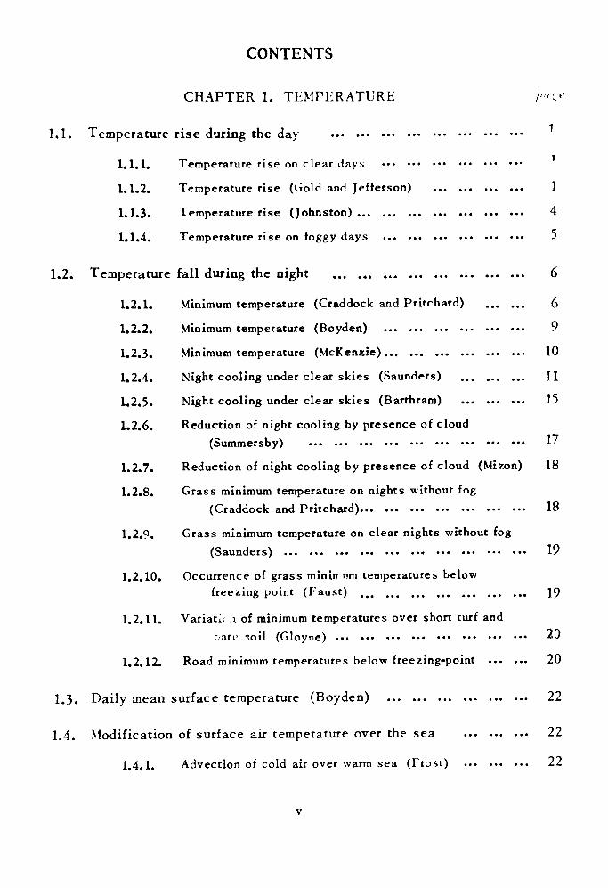
CONTENTS
CHAPTER 1. TEMPERATURE /"<;;••
1.1. Temperature rise during the day ..• ••• ••• «•• ••• ••• ••• ••• 1
1.1.1. Temperature rise on clear days ••• ••« ••• ... ••• ««•
1.1.2. Temperature rise (Gold and Jefferson) ... ... ... ... 1
1.1.3. Temperature rise (Johnston) ... ... ... ... ... ... ... 4
1.1.4. Temperature rise on foggy days ... ... ... ... ... ... 5
1.2. Temperature fall during the night ... ... ... ... ... ... ... ... 6
1.2.1. Minimum temperature (Craddock and Pritchard) ... ... 6
1.2.2. Minimum temperature (Boyden) ... ... ... ... ... ... 9
1.2.3. Minimum temperature (McKenzie) ... ... ... ... ... ... 10
1.2.4. Night cooling under clear skies (Saunders) ... ... ... H
1.2.5. Night cooling under clear skies (Barthram) ... ... ... 15
1.2.6. Reduction of night cooling by presence of cloud(Summersby) ... ... ... ... ... ••• ••« «•• ••• 17
1.2.7. Reduction of night cooling by presence of cloud (Mi?.on) 18
1.2.8. Grass minimum temperature on nights without fog(Craddock and Pritchard)... ... ... ... ... ... ... 18
1.2.9. Grass minimum temperature on clear nights without fog
(Saunders) ... ... ... ... ... ... ... ... ... ... 19
1.2.10. Occurrence of grass minimim temperatures below
freezing point (Faust) ... ... ... ... ... ... ... 19
1.2.11. Variation of minimum temperatures over short turf andhare soil (Gloyne) ... ... ... ••• ««• ••• ••> ••• 20
1.2.12. Road minimum temperatures below freezing-point ... ... 20
1.3. Daily mean surface temperature (Boyden) ... ... ... ... ... ... 22
1.4. Modification of surface air temperature over the sea ... ... ... 22
1.4.1. Advection of cold air over warm sea (Frost) ... ... ... 22
page
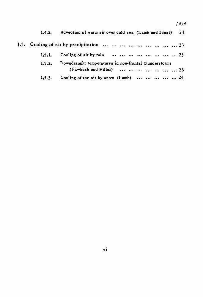
1.4.2. Advection of warm air over cold sea (Lamb and Frost) 23
1.5. Cooling of air by precipitation ... ... ... ... ... ... ... ... ... 23
1.5.1. Cooling of air by rain ••• ••• ••• ... ••• ... ... ... 23
1.5.2. Downdraught temperatures in non-frontal thunderstorms(Fawbush and Miller) ... ... ... ... ... ... ... 23
1.5.3. Cooling of the air by snow (Lumb) ... ... ... ... ... 24
VI
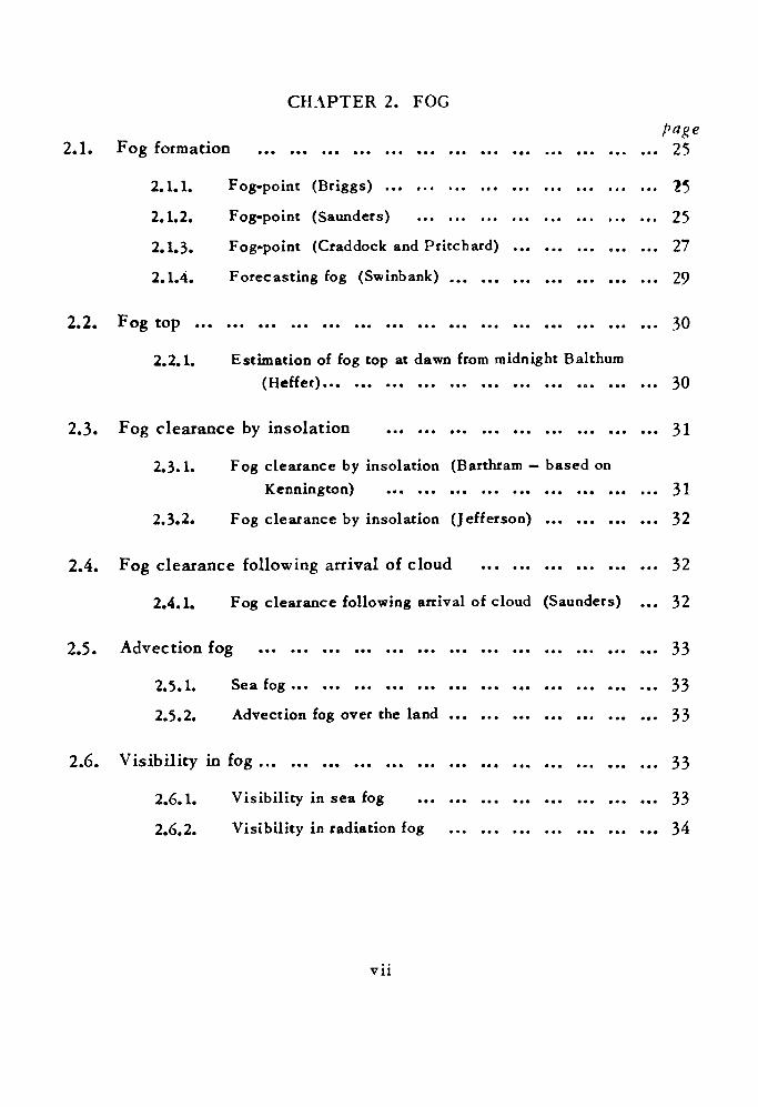
CHAPTER 2. FOG
2.1. Fog formation ... ... ... ... ... ... ... ... ... ... ... ... ... 25
2.1.1. Fog-point (Briggs) ... ... ... ... ... ... ... ... ... ?5
2.1.2. Fog-point (Saunders) ... ... ... ... ... ... ... ... 25
2.1.3. Fog-point (Craddock and Pritchard) ... ... ... ... ... 27
2.1.4. Forecasting fog (Swinbank) ... ... ... ... ... ... ... 29
2.2. Fog top ... ... ... ... ... ... ... ... ... ... ... ... ... ... ... 30
2.2.1. Estimation of fog top at dawn from midnight Balthum(Heffer)... ... ... ... ... ... ... ... ... ... ... 30
2.3. Fog clearance by insolation ... ... ... ... ... ... ... ... ... 31
2.3.1. Fog clearance by insolation (Barthram — based onKennington) ... ... ... ... ... ... ... ... ... 31
2.3.2. Fog clearance by insolation (Jefferson) ... ... ... ... 32
2.4. Fog clearance following arrival of cloud ... ... ... ... ... ... 32
2.4.1. Fog clearance following arrival of cloud (Saunders) ... 32
2.5. Advection fog ... ... ... ... ... ... ... ... ... ... ... ... ... 33
2.5.1. Sea fog... ... ... ... ... ... ... ... ... ... ... ... 33
2.5.2. Advection fog over the land ... ... ... ... ... ... ... 33
2.6. Visibility in fog ... ... ... ... ... ... ... ... ... ... ... ... ... 33
2.6.1. Visibility in sea fog ... ... ... ... ... ... ... ... 33
2.6.2. Visibility in radiation fog ... ... ... ... ... ... ... 34
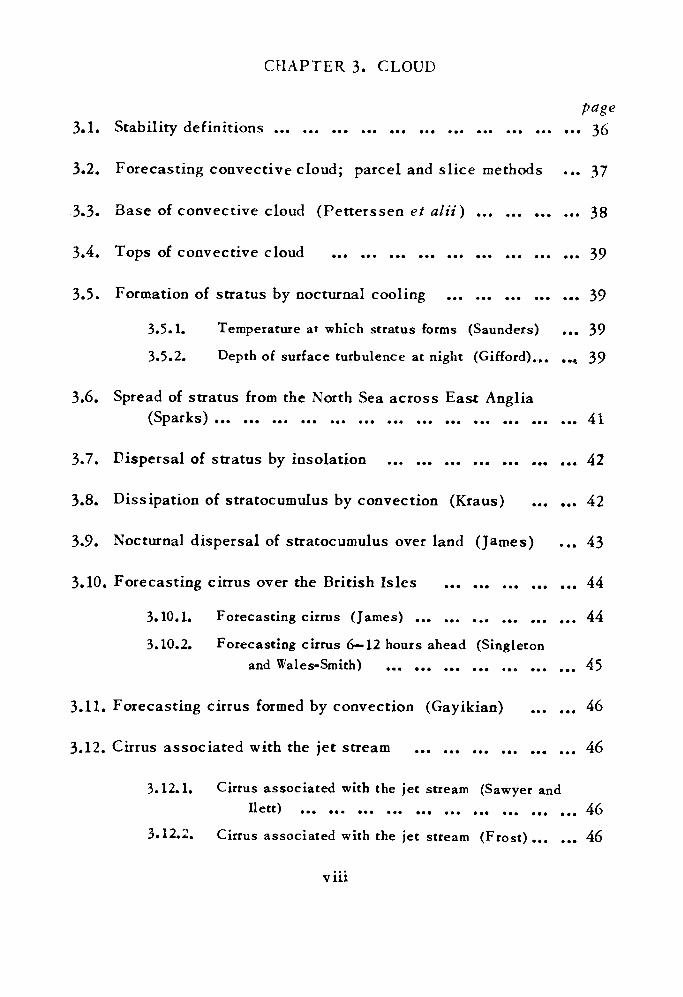
CHAPTER 3. CLOUD
page3.1. Stability definitions ... ... ... ... ... ... ... ... ... ... ... 36
3.2. Forecasting convective cloud; parcel and slice methods ... 37
3.3. Base of convective cloud (Petterssen et alii) ... ... ... ... 38
3.4. Tops of convective cloud ... ... ... ... ... ... ... ... ... 39
3.5. Formation of stratus by nocturnal cooling ... ... ... ... ... 39
3.5.1. Temperature at which stratus forms (Saunders) ... 39
3.5.2. Depth of surface turbulence at night (Gifford).,. .„ 39
3.6. Spread of stratus from the North Sea across East Anglia(Sparks) ... ... ... ... ... ... ... ... ... ... ... ... ... 41
3.7. Dispersal of stratus by insolation ... ... ... ... ... ... ... 42
3.8. Dissipation of stratocumulus by convection (Kraus) ... ... 42
3.9. Nocturnal dispersal of stratocumulus over land (James) ... 43
3.10. Forecasting cirrus over the British Isles ... ... ... ... ... 44
3.10.1. Forecasting cirrus (James) ... ... ... ... ... ... 44
3.10.2. Forecasting cirrus 6—12 hours ahead (Singletonand Wales-Smith) ... ... ... ... ... ... ... 45
3.11. Forecasting cirrus formed by convection (Gayikian) ... ... 46
3.12. Cirrus associated with the jet stream ... ... ... ... ... ... 46
3.12.1. Cirrus associated with the jet stream (Sawyer andIlett) ... ... ... ... ... ... ... ... ... ... 46
3.12.2. Cirrus associated with the jet stream (Frost)... ... 46
viii
3.13. Height of base and tops of cirrus ... ... ... ... ••• •«• ••« 47
3.13.1. Height of base and top of cirrus (Murgatroyd andGoldsmith) ... ... ... ... ... ... ... ... ... 17
3.13.2. Height of base and top of cirrus (Gayikian) ••• ... 47
3.14. The lowering of cloud base during continuous rain (Goldman) 48
IX
CHAPTER 4. UINDSpage
4.1. Geostrophic wind ... ... ... ... ... ... ... ... ... ... ... 49
4.2. Ageostrophic effects ... ... ... ... ... ... ... ... ... ... 49
4.3. Gradient wind correction ... ... ... ... ... ... ... ... ... 52
4.4. Surface wind (Findlater et alii) ... ... ... ... ... ... ... 53
4.5. Variation of wind speed in the lowest few hundred feet overfairly level ground ... ... ... ... ... ... ... ... ... ... 56
4.5.1. Variation with height when winds are strong (Shellard) 55
4.5.2. Variation according to lapse rate (Frost)... ... ... 53
4.6. Gusts near the surface (Shellard) ... ... ... ... ... ... ... 53
4.7. Forecasting peak wind gusts in non-frontal thunderstorms(Fawbush and Miller) ... ... ... ... ... ... ... ... ... 59
4.8. Gust variation with height up to about 500 feet (Deacon) ... 61
CHAPTER 5. UPPER AIR AND SURFACE CHARTS page
5.1. Phraseology ... ... ... ... ... ... ... ... ... ... ... ... ... 62
5.1.1. Zonal and meridional flow ... ... ... ... ... ... 62
5.1.2. Jet cores and jet axes ... ... ... ... ... ... ... 62
5.1.3. Long and short waves ... ... ... ... ... ... ... 62
5.1.4. Progression and retrogression ... ... ... ... ... 62
5.1.5. Trough extension and relaxation ... ... ... ... ... 62
5.1.6. Trough disruption ... ... ... ... ... ... ... ... 63
5.1.7. Blocking ... ... ... ... ... ... ... ... ... ... 6*
5.1.8. Confluence and diffluence ... ... ... ... ... ... 63
5.1.9. Divergence and convergence ... ... ... ... ... ... 64
5.1.10. Vorticity ... ... ... ... ... ... ... ... ... ... 64
5.1.11. Barotropic and baroclinic atmospheres ... ... ... 65
5.1.12. Ana-front and kata-front ... ... ... ... ... ... ... 65
5.2. Jet-stream analysis ««• ••• ••• ••• ••• ••• ••• •«• ... «•• ... 66
5.2.1. Average position of jet relative to surface fronts ... 66
5.2.2. Position of jet stream relative to thickness lines ... 67
5.2.3. Position of jet axis relative to contour lines ... ... 67
5.2.4. Vertical shear ... ... ... ... ... ... ... ... ... 67
5.2.5. Mean horizontal shear ... ... ... ... ... ... ... 68
5.2.6. Extreme cyclonic shear ... ... ... ... ... ... ... 68
5.2.7. Extreme anticyclonic shear ... ... ... ... ... ... 68
5.2.8. Indirect circulations associated with jet streams ... 69
5.3. Contour and thickness patterns ••• ••• ••• •«• ... ••• ««« •«• 69
5.3.1. Instability of zonal flow... ... ... ••• ... ... ... 69
5.3.2. Trough and ridge movement (Rossby) ... ... ... 70
5.3.3. Cut-off highs ... ... — — ••• ... ... ... ... 71
xi
5.3.4. Cut-off lows... ... ... ... ... ... ... ... ••• ... ••• 71
5.3.5. Meridional extension of thermal troughs ... ... ... ... 72
5.3.6. Relaxation of thermal troughs ... ... ... ••• ... ... 73
5.4. Relationship of surface features to 500-mb contour patterns ... 73
5.4.1. Upper low ... ... ... ... ... ... ... ... ... ... ... 73
5.4.2. Upper trough ... ... ... ... ... ... ... ... ... ... 74
5.4.3. Upper high ... ... ... ... ... ... ... ... ... ... ... 74
5.4.4. Upper ridge ... ... ... ... ... ... ... ... ... ... ... 74
5.4.5. Broad zonal flow ... ... ... ... ... ... ... ... ... 74
5.4.6. Jet axis... ... ... ... ... ... ... ... ... ... ... ... 74
5.5. Relationship of surface features to 1000 — 500 mb thicknesspatterns — ••• ••• ••• ••• ••• ••• ••• ••• ••• ••• ••• ••• ••• 75
5.5.1. Frontal depressions •«• «•« ««• ««« ••• ••• ••• ••• ••• 75
5.5.2. Anticyclones ... ... ... «•• •«• «•• ••« ««• ... ••• 75
5.6. Use of upper air charts in forecasting development and movementof surface pressure systems... ... ••• ... ... ••• ... ... ... 75
5.6.1. Sutcliffe development patterns on thickness charts ... 75
5.6.2. Deepening of depressions over the Atlantic north of 35°N(George) ... ... ... ... ... ... ... ... ... ... 77
5.6.3* Movement of warm-sector depressions ... ... ... ... 78
5.6.4. Movement of occluded and filling depressions ... ... ... 78
5.6.5. Warm-front waves and triple-point secondaries on warmocclusions ... ••• ... ••• ... ... ... ... ... ... 79
5.6.6. Cold-front waves •«« ••• ••• «•« ««• «•• ... ... ... 80
5.6.7. Triple-point secondaries on cold occlusions ••• ... ... 80
5.6.8. Surface developments linked to jet streams ••• •*• >•• 81
5.6.9. Formation of new anticyclones •«« •«• •«« «•• ... ... 81
xii
page5.6.10. Movement of anticyclones ... ... ... ... ... ... ... 84
5.6.11. Decay of anticyclones ... ... ... ... ... ... ... 84
5.7. Surface fronts ... ... ... ... ... ... ... ... ... ... ••• ... 85
5.7.1. Analysis — use of hodographs ... ... ... ... ... ... 85
5.7.2. Cold fronts (Sansom)... ... ... ... ... ... ... ... 87
5.7.3. Speed of movement of warm fronts (and warm occlusions) 87
5.7.4. Movement of cold fronts (and cold occlusions) ... ... 88
xill
CHAPTER 6. PRECIPITATIONpage
6.1. General principles ... ... ... ... ... ... ... ... ... ... &9
6.1.1. Dynamical ascent; use of contour/thickness charts 89
6.1.2. Moisture: use of tephigrams and 700-mb dew-pointdepression charts ... ... ... ... ... ... "'
6.1.3. Existing precipitation; use of satellitenephanalyses ... ... ... ... ... ... ... ™
6.2. Frontal precipitation ... ... ... ... ... ... ... ... ... "1
6.2.1. General approach ... ... ... ... ... ... ... "1
6.2.2. Warm fronts ... ... ... ... ... ... ... ... 92
6.2.3. Cold fronts ... ... ... ... ... ... ... ... 93
6.3. Precipitation at the ground from non-frontal layer cloud "4
6.3.1. Northern Ireland investigation (Mason and Howarth) '4
6.3.2. Met. R.F. investigation over central England ... 95 (Stewart) ... ... ... ... ... ... ... ... 95
6.4. Convective precipitation ... ... ... ... ... ... ... ... 95
6.4.1. General approach ... ... ... ... ... ... ... 95
6.4.2. Cloud-top temperatures «., ... .«. «,. ... ... 96
6.4.3. Cloud depth ... ... ... ... ... ... ... ... 966.4.4. Effect of vertical wind shear ... ... ... ... 96
6.4.5. Effects of local topography ... ... ... ... ... 97
6.4.6. Hail (excluding soft hail) ... .., ... ... ... 97
6.4.7. Thunderstorms ... ... ... ... ... ... ... ... 98
6.4.8. Severe Local Storms ... ... ... ... ... ... 99
6.5. Form of precipitation snow and sleet ... ... ... ... 102
6.5.1. General approach .... ... ... .^ ... .... ... 102
6.5.2. Surface dry-bulb temperature ... ... ... ... ... 102
xiv
page6.5.3. Freezing level ... ... ... ... ... ... ... ... 102
6.5.4. Wet-bulb freezing level ... ... ... ... ... ... 102
6.5.5. Downward penetration of snow... ... ... ... ... 103
6.5.6. 1000 - 500 mb thickness (NW Europe) ... ... ... 103
6.5.7. 1000 - 700 mb thickness ... ... ... ... ... ... 104
6.5.8. 1000 - 850 mb thickness ... ... ... ... ... ... 104
6.6. Summer dry spells in south-east England ... ... ... ... ... 104
6.6.1. Amplifying wave model (Lowndes)... ... ... ... 105
6.6.2. Right exit model (Ratcliffe) ... ... ... ... ... 105
6.6.3. Blocking high model (Ratcliffe and Collison) ... 106
6.7. Summer dry spells in south-west Scotland (Ratcliffe) ... 107
6.7.1. Right exit model ... ... ... ... ... ... ... ... 107
6.7.2. Blocking high model ... ... ... ... ... ... ... 108
6.8. Wet spells in south-east England ... ... ... ... ... ... ... 108
6.8.1. Left exit model (Ratcliffe and Parker) ... ... ... 108
6.8.2. Trough model (Lowndes) ... ... ... ... ... ... 109
6.9. Rapid reference guide to forecasting of precipitation ... 110
xv
CHAPTER 7. TROPOPAUSE AND STRATOSPHERE
7.1. Definition and structure of the tropopause
7.1.1. WMO definition ... ... ... ...
7.1.2. Tropopause model ... ... ...
7.2. Tropopause identification ... ... ... ... ... ... ... ••• ««• •«« ^2
7.2.1. Tropopause pressure/temperature relationship ... ... ... 7 12
7.2.2. Time changes of tropopause potential temperature andpressure •*. ... ... ... ... ... ... ... ... ... 112
7.3. Synoptic aids to the construction of tropopause charts ... ... ••• 113
7.4. The stratosphere... ... ... ... ... ... ... ... ... ... ... ... ... 114
7.4.1. ICAO standard atmosphere (ISA) ... ... ... ... ... ... 114
7.5. The lower and middle stratosphere over the British Isles in summer 114
7.6. The lower and middle stratosphere in winter*.. ••• ••• ••• «•• ••• 116
7.6.1. Major disturbances in the stratosphere ••« ••• ••• •«« 116
7.6.2. Mean values of wind and temperature over the British Isles 117
7.6.3. Data for an undisturbed winter, January 1967 at Crawley 117
7.6.4. Data for a disturbed winter, January 1968 at Crawley . .. 119
7.7. The stratosphere during the transition seasons ... ... ... ... ... 12C
7.7.1. The change from summer to winter ... ... ... ... ... 120
7.7.2. The change from winter to summer ... ... ... ... 121
xvi
CHAPTER 8. BUMPINESS IN AIRCRAFTpage
8.1. Sources and scales of turbulence ... ... ... ... ... _.. ... 122
8.2. Thermal turbulence ... ... ... ... ... ... ... ... ... ... ... 122
8.2.1. Occurrence ... ... ... ... ... ... ... ... ... ... 122
8.2.2. Typical vertical currents (based on aircraft reports) 123
8.2.3. Forecasting intensity of turbulence in cloud from the
tephigram (George) ... ... ... ... ... ... ... 124
8.3. Dynamical turbulence ... ... ... ... ... ... ... ... ... ... 124
8.3.1. Association with synoptic features ... ... ... ... 125
8.3.2. Effect of topography... ... ... ... ... ... ... ... 126
8.4. Orographic turbulence ... ... ... ... ... ... ... ... ... ... 126
8.4.1. Low-level turbulence ... ... ... ... ... ... ... 126
8.4.2. Squalls near the surface ... ... ... ... ... ... 126
8.4.3. Mountain waves ... ... ... ... ... ... ... ... ... 127
8.4.4. Rotor-zone turbulence ... ... ... ... ... ... ... 127
xv 11
CHAPTER 9. ICE ACCRETION ON AIRCRAFT page
9.1. Types of icing ... ... ... ... ... ... ... ... ... ... ••• ••• 128
9.2. General remarks ... ... ... ... ... ... ... ... •*• ... ••• ••• 128
9.3. Kinetic heating effects ... ... ... ... ... ... ... ... ... ... 129
9.4. Variation with cloud type ... ... ... ... ... ... ... ... ... 130
9.5. Cloud properties and icing risk ... ... ... ... ... ... ... ... 130
9.5.1. Convective clouds (Cu and Cb) ... ... ... ... ... 130
9.5.2. Non-frontal layer clouds (St, Sc and Ac) ... ... ... 131
9.5.3. Frontal layer cloud ... ... ... ... ... ... ... ... 1329.5.4. Ice-crystal clouds ... ... ... ... ... ... ... ... 132
9.5.5. Orographic cloud ... ... -.. ... ... ... ... ... 132
9.6. Icing associated with fronts and precipitation ... ... ... ... 133
9.6.1. Warm fronts ... ... ... ... ... ... ... ... ... ... 133
9.6.2. Cold fronts ... ... ... ... ... ... ... ... ... ... 133
9.6.3. Depressions with ill-defined fronts ... ... ... ... 133
9.7. Engine icing ... ... ... ... ... ... ... ... ... ... ... ... ... 133
9.8. Helicopter icing ... ... ... ... ... ... ... ... ... ... ... ... 134
xv ni
CHAPTER 10. CONDENSATION TRAILS (CONTRAILS)page
10.1. Forecasting exhaust contrails from jet aircraft ... ... ... 135
10.1.1. Helliwell and Mackenzie's method ... ... ... ... 135
10.1.2. Appleman's method... ... ... ... ... ... ... ... 135
10.2. Estimating the humidity ... ... ... ... ... ... ... ... ... 136
xix
APPENDIX 1page
Table I Solar altitude at midday, times of sunrise and sunset... 137
II Coriolis parameter... ... ... ... ... ... ... ... ... ... 138III Rossby long waves ••• ••• ••• ••• ••• ••• ••• ••• ••• 138
IV Temperature conversion ... ... ... ... ••• ... ••• •«• 139
V Water vapour density, saturation vapour pressure ••• ••• 140
VI ICAO atmosphere (dry air) ... ... ... ... ... ... ... ... 141
APPENDIX 2
1. Geopotential ... ... ... ... ... ... ... ... ... ... ••• 143
2. Equation of state ... ... ... ... ... ... ... ... ... ... 1433. Hydrostatic equation ... ... ... ... ... ... ... ... ... 1444. Thermodynamics ... ... ... ... ... ... ... ... ... ... 145
5. Water vapour ... ... ... ... ... ... ... ... ... ... ... 1456. Equation of continuity ... ... ... ... ... ... ... ... ... 1467. Equations of motion ... ... ... ... ... ... ... ... ... 147
8. Vorticity ... ... ... ... ... ... ... ... ... ... ... ... 1499. Radiation ... ... ... ... ... ... .,. ... ... ... ... ... 151
10. Miscellaneous constants and relations ... ... ... ... 152
xx
CHAPTER 1. TEMPERATURE 1.1. TEMPERATURE RISE DURING THE DAY1.1.1. Temperature rise on clear days
Alternative methods are given in 1.1.2. and 1.1.3- for estimating the rise of temperature at the surface after dawn on clear days. For both methods it is necessary to start with a tephigram on which is plotted a dawn temperature curve (actual or estimated) for the lowest few thousand feet of the air which will lie over the forecast area at the appropriate time during the morning or early afternoon. If cloud develops, an esti mate has to be made of the reduction in the value of the temperatures as forecast by either method.
It should be noted that the values given in Tables I.I. and l.II. apply to southern England.
1.1.2. Temperature rise (Gold and Jefferson)
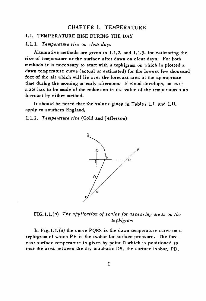
FIG.l.l.(tf) The application of scales for assessing areas on thetephigram
In Fig. 1. l.(a) the curve PQRS is the dawn temperature curve on a tephigram of which PE is the isobar for surface pressure. The fore cast surface temperature is given by point D which is positioned so tbat the area between the dry adiabatic DR, the surface isobar, PD,
16141210
8
B
A'
1412
BD'
A'
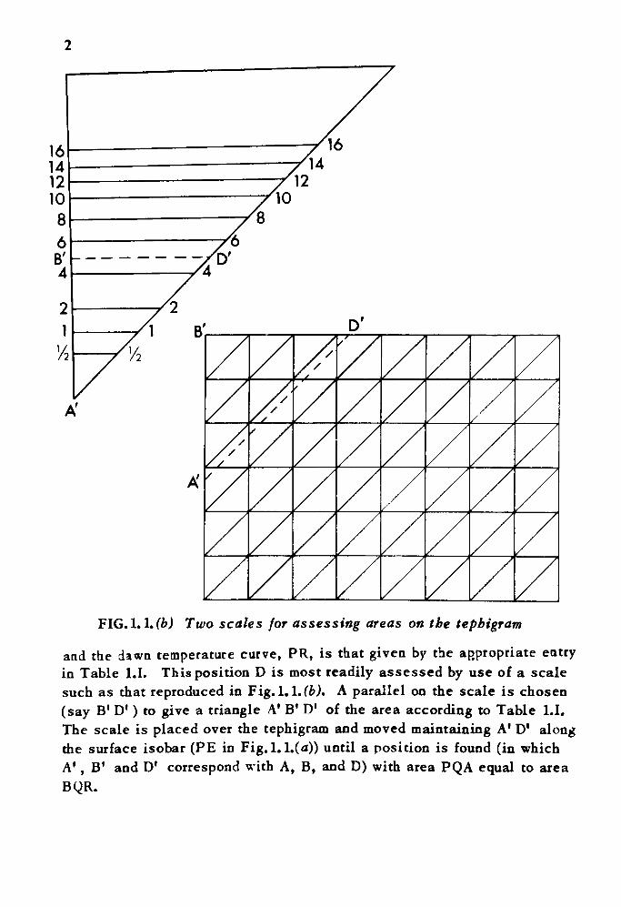
FIG. 1.1.ft) Tu;o scales for assessing areas on the tepbigtam
and the dawn temperature curve, PR, is that given by the appropriate entry in Table I.I. This position D is most readily assessed by use of a scale such as that reproduced in Fig. 1.1. (b). A parallel on the scale is chosen (say B 1 D 1 ) to give a triangle A 1 B 1 D 1 of the area according to Table I.I. The scale is placed over the tephigram and moved maintaining A 1 D1 along the surface isobar (PE in Fig. 1.!.(«)) until a position is found (in which A 1 , B 1 and D 1 correspond with A, B, and D) with area PQA equal to area BQR.
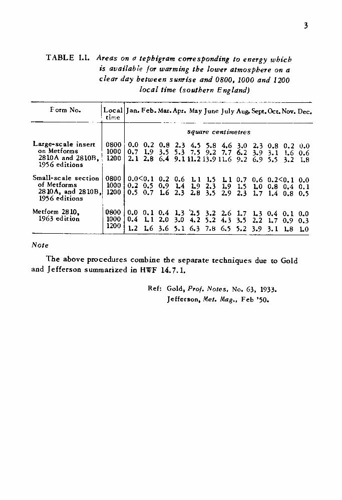
TABLE 1.1. Areas on a tephigram corresponding to energy which is available for warming the lower atmosphere on a clear day between sunrise and 0800, 1000 and 1200
local time (southern England)
Form No.
Large-scale insert on Metforms 28 10 A and 2810B, 1956 editions
Small-scale section of Metforms 28 10 A, and 2810B, 1956 editions
Metform 2810, 1963 edition
Localtime
0800 1000 1200
0800 1000 1200
0800 1000 1200
Jan. Feb. Mar. Apr. May June July Aug. Sept. Oct. Nov. Dec.
square centimetres
0.0 0.2 0.8 2.3 4.5 5.8 4.6 3.0 2.3 0.8 0.2 0.0 0.7 1.9 3.5 5.3 7.5 9.2 7.7 6.2 3.9 3.1 1.6 0.6 2.1 2.8 6.4 9.111.213.911.6 9.2 6.9 5.5 3.2 1.8
0.0<0.1 0.2 0.6 LI 1.5 LI 0.7 0.6 0.2<0. 1 0.0 0.2 0.5 0.9 L4 L9 2.3 L9 1.5 LO 0.8 0.4 0.1 0.5 0.7 1.6 2.3 2.8 3.5 2.9 2.3 1.7 1.4 0.8 0.5
0.0 0.1 0.4 1.3 '2.5 3.2 2.6 1.7 L3 0.4 0.1 0.0 0.4 LI 2.0 3.0 4.2 5.2 4.3 3.5 2.2 1.7 0.9 0.3 1.2 L6 3.6 5.1 6.3 7.8 6.5 5.2 3.9 3.1 1.8 1.0
Note
The above procedures combine the separate techniques due to Gold and Jefferson summarized in HWF 14.7.1.
Ref: Gold, Prof. Notes, No. 63, 1933. Jefferson, Met. Mag., Feb '50.
1.1.3. Temperature rise (Johnston)
TABLE l.II. Thickness of layer which is changed from an isothermal to an adiabatic state by insolation (southern England)
Month
Jan.Feb.Mar.Apr.MayJuneJulyAug.Sept.Oct.Nov.Dec.
1 2 3BOUTS from
4 5
sunrise 6789
millibarsA B
16182022
A 23' 23
232221
A 19
1715
29 4133 4637 524042424241
5659605957
38 5435 4931 43]_28 40
50 |5763697273737066605349)
A
5865738083848481766961—
B
— — — —7382 90 -89 98 10693 102 110 11894 103 112 11994 103 111 11891 99 108 11585 93 10077 85 -_ _ _ __ _ _ _
Max.
618197
115127130125119104876153
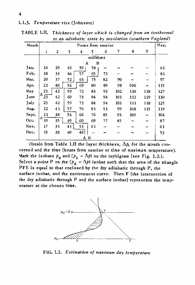
Obtain from Table l.II the layer thickness, Apt for the month con cerned and the time (hours from sunrise or time of maximum temperature). Mark the isobars p Q and (p Q - Ap) on the tephigram (see Fig. 1.2.). Select a point P on the (p Q — Ap) isobar such that the area of the triangle PFE is equal to that enclosed by the dry adiabatic through P, the surface isobar, and the environment curve. Then F (the intersection of the dry adiabatic through P and the surface isobar) represents the temp erature at the chosen time.
Po-
FIG. 1.2. Estimation of maximum day temperature
Note 5
Over damp soils, e.g. clay, the energy corresponding to the values given is not available for heating the lowest layers of the atmosphere during the first few hours of sunshine. In such localities, the values to the left of the lines marked A in Table l.II. should be reduced by one- third and the values between the lines marked A and B should be reduced by one-fifth.
Ref: HWF 14.7.1.Tohnston, Met.Mag., Sept.'58. Jefferson, Met.Mag., May '59.
1.1.4. Temperature rise on foggy days
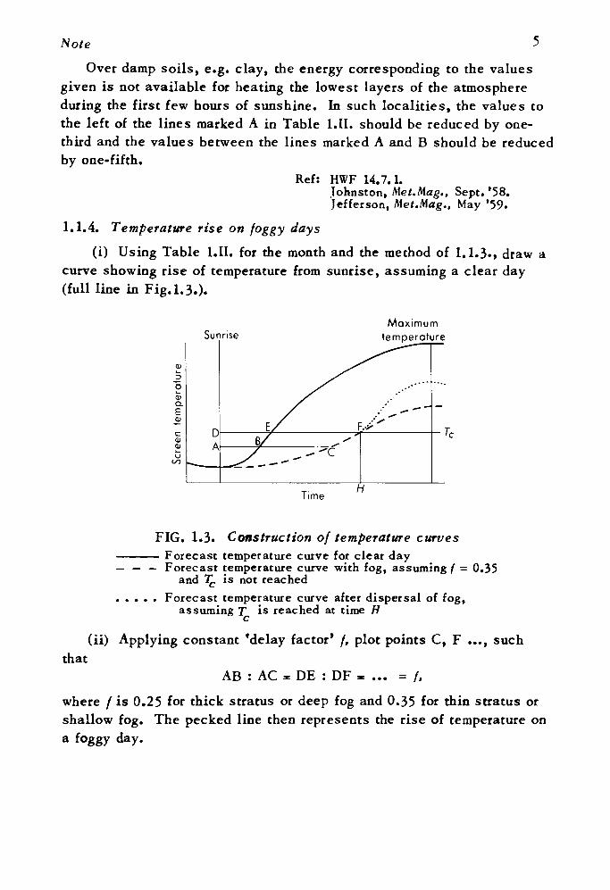
(i) Using Table l.II. for the month and the method of 1.1.3., draw a curve showing rise of temperature from sunrise, assuming a clear day (full line in Fig. 1.3.).
SunriseMaximum
temperature
Time
FIG. 1.3. Construction of temperature curvesForecast temperature curve for clear day
— — — Forecast temperature curve with fog, assuming/ = 0.35and TC is not reached
Forecast temperature curve after dispersal of fog, assuming T 'ls reached at time H
(ii) Applying constant 'delay factor' /, plot points C, F ..., suchthat
AB : AC - DE : DF = /.
where /is 0.25 for thick stratus or deep fog and 0.35 for thin stratus or shallow fog. The pecked line then represents the rise of temperature on a foggy day.
6(iii) If this curve reaches temperature, T , at which fog can be
expected to disperse (see 2.6.)t £he curve then rises more steeply and is more in line with clear-day characteristics (e.g. dotted line in Fig. 1.3.).
Notes(a) On a particular occasion, / can be evaluated from an observation
of temperature made not less than 3h after sunrise. If /., is the time at which the temperature was observed, tl the time (estimated by method of (i)) at which the same temperature would have been reached on a clear day, and t Q is the time of sunrise, then /= (t l - tQ )/(t 2 - tQ ).
(b) A diagram similar to Fig. 1.3. is used for estimating the time of clearance of radiation fog or low stratus (see 2.6.).
Ref: HWF 17.8.Jefferson, Met.Mag., Apr.'50.
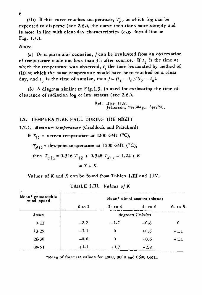
1.2. TEMPERATURE FALL DURING THE NIGHT 1.2.1. Minimum temperature (Craddock and Pritchard)
If T12 = screen temperature at 1200 GMT (°C),
Tj| 2 = dew-point temperature at 1200 GMT (°C),
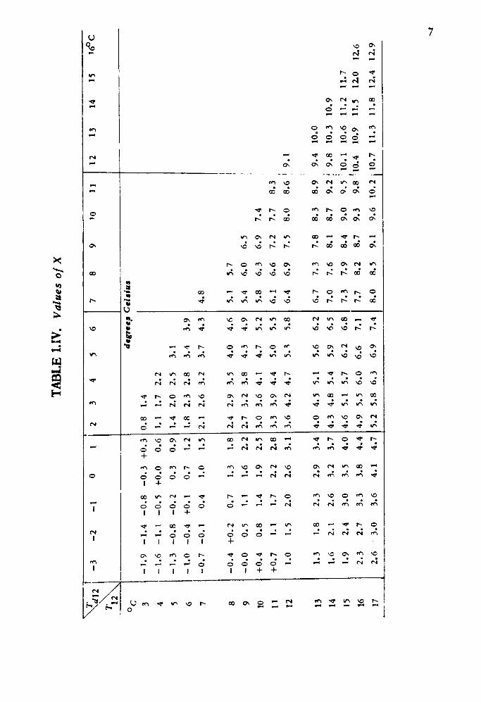
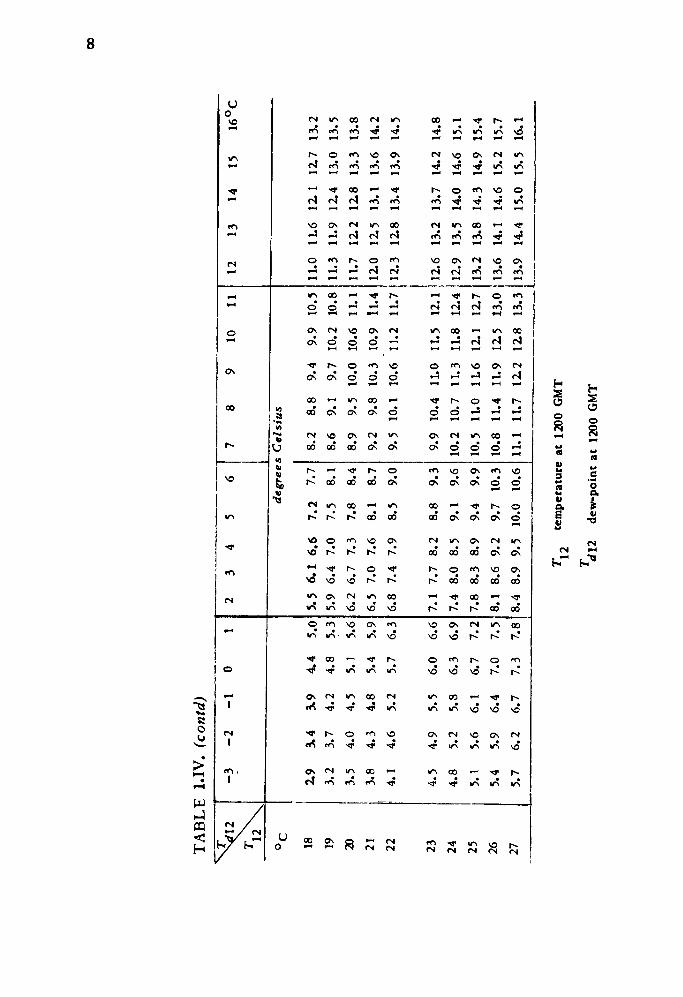
then T . = 0.316 T., + 0.548 TV, - 1.24+ K nun \.L u\ L« X + K.
Values of K and X can be found from Tables l.HI and l.IV.
TABLE l.HI. Values of K
Mean* geostrophic wind speed
knots
0-12
13-25
26-38
39-51
Mean* cloud amount (oktas)
0 to 2
-2.2
-1.1
-0.6
+ 1.1
2+ to 4
degrees
-1.7
0
0
+ 1.7
4+ to 6
Ce Is ius
-0.6
+0.6
+0.6
+ 2.8
6+ to 8
0
+ 1.1
+ 1.1
•Mean of forecast values for 1800, 0000 and 0600 GMT.
TABL
E 1.
IV.
Valu
es o
f X
\r
I
°c 3 4 5 6 7 8 9 10 11 12 13 14 15 16 17
-3 -1.9
-1.6
-1.3
-1.0
-0.7
-0.4
-0.0
+0.
4
+0.
71.
0
1.3
1.6
1.9
2.3
2.6
-2
-I
-1.4
-0
.8-1
.1
-0.5
-0.8
-0
.2-0
.4
+0.
1
-0.1
0.
4
+0.
2 0.
70.
5 1.
10.
8 1.
41.
1 1.
7
1.5
2.0
1.8
2.3
2.1
2.6
2.4
3.0
2.7
3.3
3.0
3.6
0
-0.3
+0.
00.
3
0.7
1.0
1.3
1.6
1.9
2.2
2.6
2.9
3.2
3.5
3.8
4.1
——
——
r 1
+0.
3
0.6
0.9
1.2
1.5
1.8
2.2
2.5
2.8
3.1
3.4
3.7
4.0
4.4
4.7
234
0.8
1.4
1.1
1.7
2.2
1.4
2.0
2.5
1.8
2.3
2.8
2.1
2.6
3.2
2.4
2.9
3.5
2.7
3.2
3.8
3.0
3.6
4.1
3.3
3.9
4.4
3.6
4.2
4.7
4.0
4.5
5.1
4.3
4.8
5.4
4.6
5.1
5.7
4.9
5.5
6.0
5.2
5.8
6.3
56
degr
ees
3.1
3.4
3.7
4,0
4.3
4.7
5.0
5.3
5.6
5.9
6.2
6.6
6.9
3.9
4.3
4.6
4.9
5.2
5.5
5.8
6.2
6.5
6.8
7.1
7.4
7
Cel
sius
4.8
5.1
5.4
5.8
6.1
6.4
6.7
7.0
7.3
7.7
8.0
8 5.7
6.0
6.3
6.6
6.9
7.3
7.6
7.9
8.2
8.5
9 10
11
12
13
14
15
16°C
f
6.5
6.9
7.4
7.2
7.7
8.3
7.5
8.0
8.6
9.1
7.8
8.3
8.9
9.4
10.0
8.1
8.7
9.2
j 9.
8 10
.3
10.9
8.4
9.0
9.5
;10.1
10
.6
11.2
11
.78.
7 9.
3 9.
8 'l0
.4
10.9
11
.5
12.0
12
.6
9.1
9.6
10. 2
j 10
. 7
11.3
11
.8
12.4
12
.9
00
TA
BL
E 1
.1 V
. (c
ontd
)
^(1
2T
N.
12\
°C 18 19 20 21 22 23 24 25 26 27
-3 2.9
3.2
3.5
3.8
4.1
4.5
4.8
5.1
5.4
5.7
-2 3.4
3.7
4.0
4.3
4.6
4.9
5.2
5.6
5.9
6.2
-I 3.9
4.2
4.5
4.8
5.2
5.5
5.8
6.1
6.4
6.7
0 4.4
4.8
5.1
5.4
5.7
6.0
6.3
6.7
7.0
7.3
1 5.0
5.3
5.6
5.9
6.3
6.6
6.9
7.2
7.5
7.8
234
5.5
6,1
6.6
5.9
6.4
7.0
6.2
6.7
7.3
6.5
7.0
7.6
6.8
7.4
7.9
7.1
7.7
8.2
7.4
8.0
8.5
7.8
8.3
8.9
8.1
8.6
9.2
8.4
8.9
9.5
5 6
7 8
9 10
11
degr
ees
Cel
sius
7.2
7.7
7.5
8.1
7.8
8.4
8.1
8.7
8.5
9.0
8.8
9.3
9. 1
9.6
9.4
9.9
9.7
10.3
10.0
10
.6
8.2
8.8
9.4
9.9
10.5
8.6
9.1
9.7
10.2
10
.88.
9 9.
5 10
.0
10.6
11
.19.
2 9.
8 10
.3
10.9
ll
.49.
5 10
.1
10.6
11
.2
11.7
9.9
10.4
11
.0
11.5
12
.110
.2
10.7
11
.3
11.8
12
.410
.5
11.0
1L
6 12
.1
12.7
10.8
11
.4
11.9
12
.5
13.0
11.1
11
.7
12.2
12
.8
13.3
12
13
11.0
11
.611
.3
11.9
11.7
12
.212
.0
12.5
12.3
12
.8
12.6
13
.212
.9
13.5
13.2
13
.813
.6
14. 1
13.9
14
.4
14
15
12.1
12
.712
.4
13.0
12.8
13
.313
.1
13.6
13.4
13
.9
13.7
14
.214
.0
14.6
14.3
14
.914
.6
15.2
15.0
15
.5
16°C
13.2
13.5
13.8
14.2
14.5
14.8
15.1
15.4
15.7
16.1
_te
mpe
tatu
re a
t 12
00 G
MT
dl2
dew
-poi
nt
at
1200
GM
T
Notes
(a) The formula given by Craddock and Pritchard was derivH fron-. the combined data for 16 widely separated stations in England, all n-ore than 10 miles inland. For forecasting night minimum temperatures at a particular place accuracy is likely to be improved by consideration of local data, for instance local values might be found for K.
(b) The formula applies to nights without fog.
(c) If the ground is snow covered the actual minimum is likely to be lower than the minimum forecast by means of this technique or other techniques described in 1.2.
Ref: HWF 14.7. >.l.Craddock and Pritchard, MRP 624.
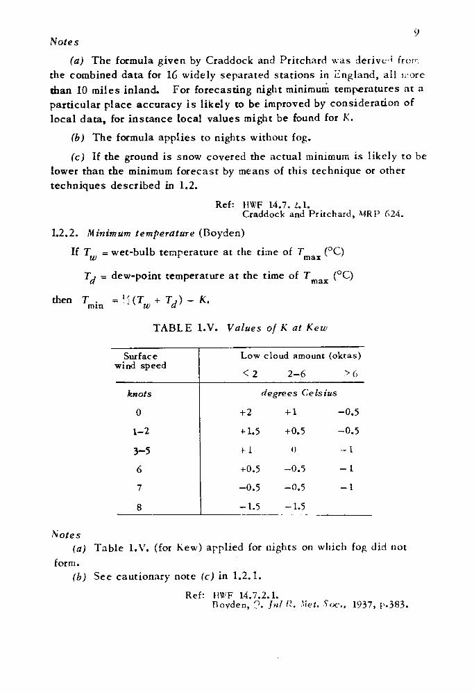
1.2.2. Minimum temperature (Boyden)
If T = wet-bulb temperature at the time of T (°C) w r max
T, = dew-point temperature at the time of Tm<tv (°C)
then T . = nun w + T,) - K.
TABLE l.V. Values of K at Kew
Surface wind speed
knots
0
1-2
3-5
6
7
8
Low
<2
cloud amount
2-6
(oktas)
>6
degrees Celsius
+ 2
+ 1.5
+ i
+0.5-0.5
-1.5
-l-l
+0.5
0
-0.5
-0.5
-1.5
-0.5
-0.5
-I
-1
-1
Notes(a) Table l.V. (for Kew) applied for nights on which fog did not
form.(b) See cautionary note (c) in 1.2.1.
Ref: HW'F 14.7.2.1.Boyden, ?. Jnl R. Met. Soc., 1937, p.383.
10
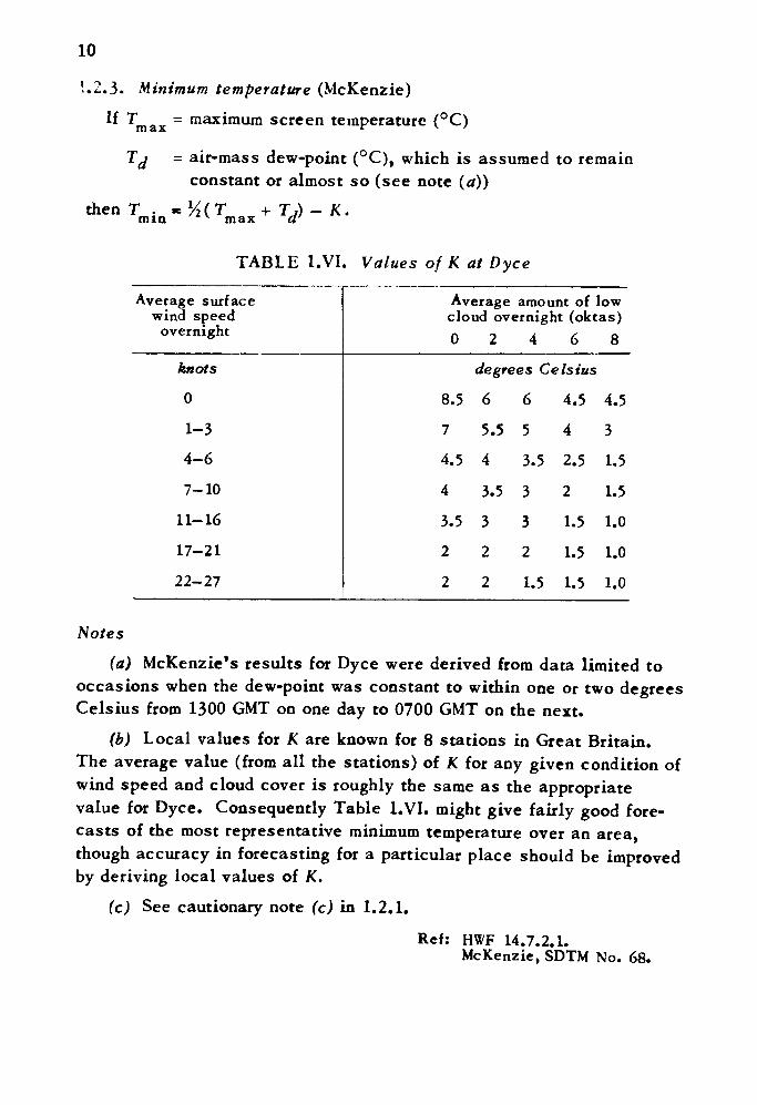
?.3. Minimum temperature (McKenzie)
If T __ = maximum screen temperature (°C)max
= air-mass dew-point (°C), which is assumed to remain constant or almost so (see note (a))
then T . - Y2 (T + T,) - K. mm v max a'
TABLE l.VI. Values of K
Average surface wind speed overnight
knots
0
1-34-6
7-10
11-16
17-21
22-27
at Dyce
Average amount of low cloud overnight (oktas)02468
8.5
7
4.5
4
3.5
2
2
degrees Celsius
6 6 4.5
5.5 5 4
4 3.5 2.5
3.5 3 2
3 3 1.5
2 2 1.5
2 1.5 1.5
4.5
3
1.5
1.5
1.0
1.0
1.0
Notes
(a) McKenzie's results for Dyce were derived from data limited to occasions when the dew-point was constant to within one or two degrees Celsius from 1300 GMT on one day to 0700 GMT on the next.
(b) Local values for K are known for 8 stations in Great Britain. The average value (from all the stations) of K for any given condition of wind speed and cloud cover is roughly the same as the appropriate value for Dyce. Consequently Table l.VI. might give fairly good fore casts of the most representative minimum temperature over an area, though accuracy in forecasting for a particular place should be improved by deriving local values of K.
(c) See cautionary note (c) in 1.2.1.
Ref: HWF 14.7.2.1.McKenzie, SDTM No. 68.
111.2.4. Night cooling under clear skies (Saunders)
(i) Consider whether the observed T and 7 ', (the dew-point atmax a '
the time of Tmax ) for the afternoon are representative of the air likely to be over the locality during the night; if they are not, make an estimate of appropriate values from observations upwind.
(ii) Estimate whether there will be an inversion base at or below 900 mb during the afternoon.
(iii) Calculate T , the temperature at the time of discontinuity in the rate of cooling, from the regression equation
Tr = '* Tmax + V ~ *•
At Northolt, K = 0.3 degC when there is no inversion with base below 900 mb and K = 2.2 degC with an inversion with base below 900 mb.
(iv) The approximate times (GMT) at which the discontinuity in cooling occurs at Northolt are:
Jan. Feb. Mar. Apr. May June July Aug. Sept. Oct. Nov. Dec.
1645 1800 1930 2045 2100 2115 2115 2045 1930 1745 1700 1630
If the tops oil is wet the discontinuity occurs about Ih earlier than given above in late spring and early summer, and about %h earlier in late summer.
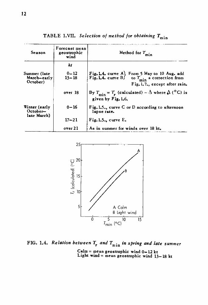
(v) Obtain T . from the forecast T, and the forecast mean mm Tgeostrophic wind speed for the period of subsequent cooling using Table l.VII. and Figs. 1.4.- 1.7.
12
TABLE l.VII. Selection of method for obtaining Tmm
Season
Summer (late March— early October)
Winter (early October- late March)
Forecast mean geostrophic
wind
0-12 13-18
over 18
0-16
17-21
over 2 1
Method for T . nun
Fig. L4. curve A\. From 5 May to 10 Aug. addFig. 1.4. curve B/ to T . a correction from0 nun
Fig. 1.7., except after rain.
By T . = T (calculated) - A where ^ (°C) mm fgiven by Fig. 1.6.
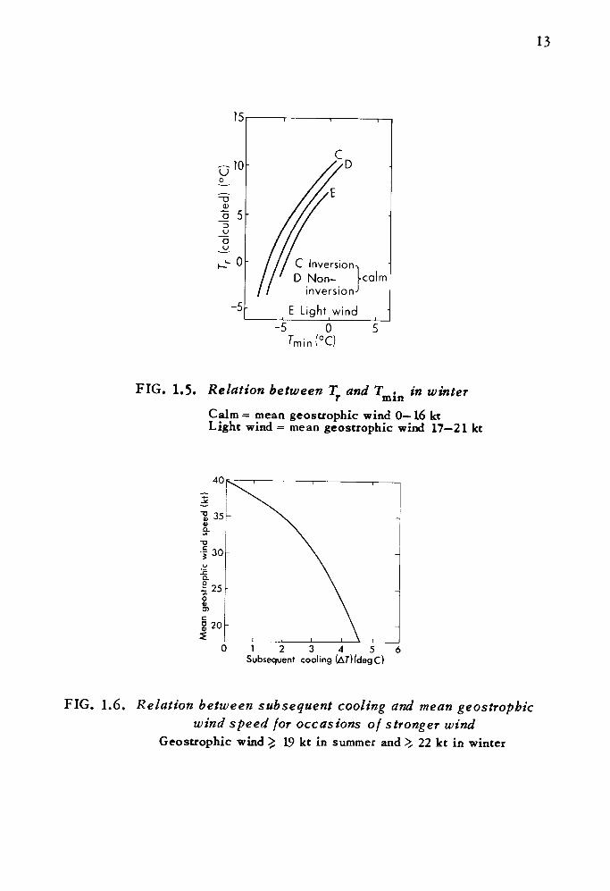
Fig. 1.5., curve C or D according to afternoon lapse rate.
Fig. 1.5., curve E.
As in summer for winds over 18 kt.
is
u
25
20
0)
Jo 153 U
0 U
mA CalB Light wind
10 15
FIG. 1.4. Relation between Tf and Tm -in in spring and late summerCalm = mean geostrophic wind 0—12 kt Light wind = mean geostrophic wind 13—18 kt
13
15
<Jo
10
oU
-5
C Inversion-,D Non- Kdlm
nverson-
E Light wind
-5 Q 0' m i n ( C)
FIG. 1.5. Relation between T and T • in winterr mmCalm = mean geostrophic wind 0—16 kt Light wind = mean geostrophic wind 17—21 kt
0123456 Subsequent cooling (ATHdegC)
FIG. 1.6. Relation between subsequent cooling and mean geostrophicwind speed for occasions of stronger wind
Geostrophic wind £ 19 kt in summer and ^ 22 kt in winter
14
2-0O
I i-o20-5 o
5 101520253051015202530510152025305 10 May June July August
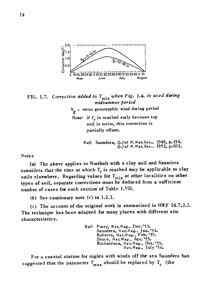
FIG. 1.7. Correction added to T • when Fig. 1.4. is used duringmm ° °
midsummer periodV = mean geostrophic wind during period
§Note: if T is reached early because top
soil is moist, this correction is partially offset.
Ref: Saunders, Q.Jnl R.Met.Soc.. 1949, p. 154. Q.Jnl R.Met.Soc.. 1952, p.603.
Notes
(a) The above applies to Northolt with a clay soil and Saunders considers that the time at which T is reached may be applicable to clay soils elsewhere. Regarding values for Tm jn at other localities on other types of soil, separate corrections must be deduced from a sufficient number of cases for each section of Table l.VII.
(b) See cautionary note (c) in 1.2.1.
(c) The account of the original work is summarized in HWF 14.7.2.2. The technique has been adapted for many places with different site characteristics.
Ref: Parry, Met.Mag., Dec.'53.Saunders, Met.Mag., Jan.'54. Roberts, Met.Mag., Feb.'55. Bruce, Met.Mag., Apr. '55. Richardson, Met.Mag.. Oct. '55.
Met.Mag., July '56.
For a coastal station for nights with winds off the sea Saunders has suggested that the parameter Tmax should be replaced by T (the
15
temperature of the sea surface) in the formula for forecasting 7_.Ref: Saunders, Met.Mag.. Mar. '55.
1.2.5. Night cooling under clear skies (Barthram)
This method is applicable to inland stations in the southern half of England (based on Saunders' s technique).
(i) If T is day maximum temperature, T> is the dew-point at
time of T , then T, the temperature at the time when there is a checkmax r rin the rate of cooling, is given by
where K = 1 degC when there is no inversion in the afternoon below 850 mb,
K = 2 degC when there is an inversion in the afternoon below 850 mb.
(ii) The times (GMT) of T. at the beginning of each month are:
Jan. Feb. Mar. Apr. May June July Aug. Sept. Oct. Nov. Dec.
1645 1745 1845 2015 2100 2130 2145 2130 2030 1900 1745 1700
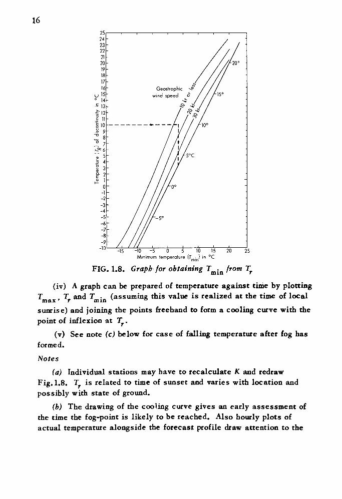
(iii) From the value of T and the forecast geos trophic wind speed during the night, Fig. 1.8. gives an estimate of the night minimum temperature (Tmin ).
1625242322212019181716
0 14113
111 §10.2 9 ~o
j! 7K*6
. 5a 4 I 3 - 2 ,• 1
0-1-2-3-4-5-6-7-8-9
-10
—i—————i—————r-
Geostrophic ^ wind speed o
-15 -10 -5 0 5 10 15 Minimum temperature (T • ) in °C
20 25
FIG. 1.8. Graph for obtaining Tmin from Tf
(iv) A graph can be prepared of temperature against time by plottingT T and T • (assuming this value is realized at the time of local max 7 r mm v °sunrise) and joining the points freehand to form a cooling curve with the point of inflexion at Tf .
(v) See note (c) below for case of falling temperature after fog has formed.
Notes(a) Individual stations may have to recalculate K and redraw
Fig. 1.8. T is related to time of sunset and varies with location and possibly with state of ground.
(b) The drawing of the cooling curve gives an early assessment of the time the fog-point is likely to be reached. Also hourly plots of actual temperature alongside the forecast profile draw attention to the
17
occasions when this forecast time may require amendment. The probable time of air frost is also readily obtained.
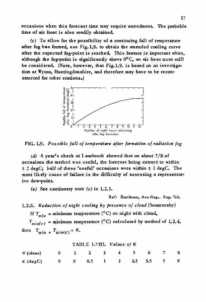
(c) To allow for the possibility of a continuing fall of temperature after fog has formed, use Fig. 1.9. to obtain the amended cooling curve after the expected fog-point is reached. This feature is important when, although the fog-point is significantly above 0°C, an air frost must still be considered. (Note, however, that Fig. 1.9. is based on an investiga tion at Wyton, Huntingdonshire, and therefore may have to be recon structed for other stations*)
12Number of night hours remaining
after fog formation
FIG. 1.9. Possible fall of temperature after formation of radiation fog
(d) A year's check at Laarbruch showed that on about 7/8 of occasions the method was useful, the forecast being correct to within ± 2 degC; half of these 'useful* occasions were within ± 1 degC. The most likely cause of failure is the difficulty of assessing a representat ive dew-point.
(e) See cautionary note (c) in 1.2.1.
Ref: Barthram, Met.Mag., Aug. '64.
1.2.6. Reduction of night cooling by presence of cloud (Summersby)
If T • » minimum temperature (°C) on night with cloud,
minimum temperature (°C) calculated by method of 1.2.4.
mn
N (oktas)
K (degC)
Tnun(c)
TABLE l.VIII. Values of K
0 12345678
0 0 0.5 1 2 2.5 3.5 5 8
18 Notes
(a) It is suggested that the above formula, based on data for Northolt, would probably be satisfactory at stations with similar sub soil and topography.
(b) Nights with precipitation are excluded.
Ref: HWF 14.7.2.3.Summersby, Met.Mag., July '53.
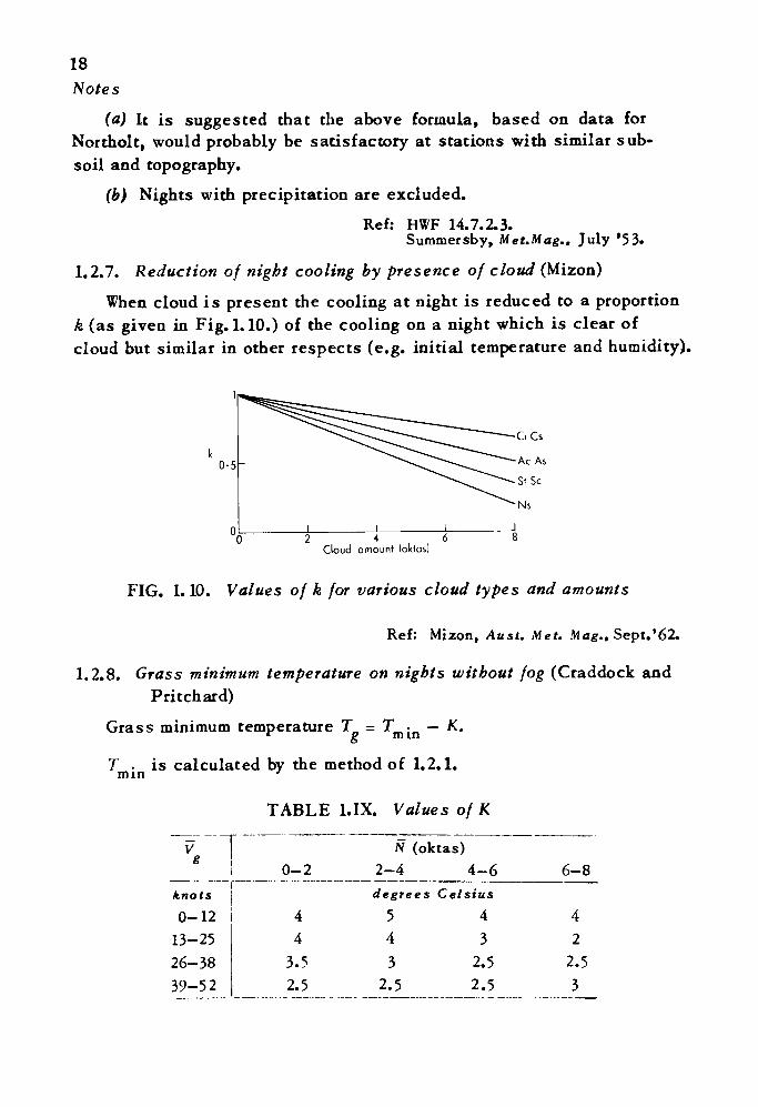
1.2.7. Reduction of night cooling by presence of cloud (Mizon)
When cloud is present the cooling at night is reduced to a proportion k (as given in Fig. 1.10.) of the cooling on a night which is clear of cloud but similar in other respects (e.g. initial temperature and humidity).
0-5
2468 Cloud amount (oktas)
FIG. 1.10. Values of k for various cloud types and amounts
Ref: Mizon, Aust. Met. Mag., Sept.'62.
1.2.8. Grass minimum temperature on nights without fog (Craddock and Pritchard)
Grass minimum temperature T = T . — K.o
T . is calculated by the method of 1.2.1.m in »nun
TABLE l.IX. Values of K
0-2N (oktas)
2-4 4-6 6-8
knots
0-12 4
13-2526-3839-52
43.52.5
degrees Celsius5 44 33 2.5
2.5 2.5
42
2.53
19V = mean of geostrophic wind speeds for 1800, 0000 and 0600
e GMT.N = mean of total cloud amounts for 1800, 0000 and 0600 GMT.
Note
Craddock and Pritchard's formula is based on data for 16 stations in England.
Ref: HWF 14.7.3.Craddock and Pritchard, MRP No.624.
1.2.9. Grass minimum temperature on clear nights without fog (Saunders)
Tg = Tmin - K-
TABLE l.X. Values of K for Northolt
Summer Wintervgkt
0-12
13-24over 24
K V
degC kt 4.5 0-166 17-244 over 24
Winter with V < 17o
+2 to -0.5 -1 to -3.5
2 4
K
degC see below
64
*-4 to -6 -6.5 to -9
5 6
T • rQmm K (degC)
V = mean geostrophic wind speed overnight.
Ref: HWF 14.7.3.Saunders, Q.Jnl R.Met.Soc., 1952, p. 603.
1.2.10. Occurrence of grass minimum temperatures below freezing point (Faust)
If the cloud amount is less than 2 oktas and the wind speed is less than 4 kt during the night, ground frost will occur if
(T+ l/2 Td ) < 17.2°C,
where T is the screen temperature and T. is the dew-point at 1400 local time.
NoteOccasionally ground frost has been experienced with (T+ /
20as high as 19°C. Therefore discretion should be used when (T + l is a little above the critical value.
Reft HWF 14.7.3.Faust, Ann. Met., Hamburg, 1949, p. 105. Jefferson, Met.Mag., Oct. '5 L James, Met.Mag., Mar. '53.
1.2.11. Variation of minimum temperatures over short turf and bare soil (Gloyne)
TABLE 1.XI. Results at Starcross, Devon, 1949-50
T . -T. mm b
T.-T b g
Mean Mean(R)
Mean Mean(R)
Jan. Feb. Mar. Apr. May June July Aug. Sept.Oct. Nov.Dec.
degrees Celsius
1.5 2 1.5 2 1.5 1 1.5 2 1.5 2 2.5 2.5 3 3.5 2.5 2.5 2.5 2 2 2.5 2.5 2.5 3.5 3.5
0.5 1 1 1.5 1.5 2 1.5 1.5 1.5 1.5 1 1 1.5 1.5 2 2.5 2.5 2.5 2.5 2 2 2.5 1.5 L5
T . = minimum temperature in screenmmT = minimum temperature at % to Y2 inch above bare soil
T = grass minimum temperatureo
Mean(R) = mean on radiation nights, defined as nights on which
Ref: Gloyne, Met.Mag.. Sept. '53.
rmin -
1.2.12. Road minimum temperatures below freezing-point
(i) Differences in the thermal properties of various road materials are generally quite small. Recent work has shown that the difference (minimum screen temperature—minimum road temperature) varies with the length of night and can be used to forecast the occurrence of road surface temperatures below freezing-point. The following regression equation was obtained for a concrete road at Watnall
M A - M R = 0.28/ - 2.9,
where M A = minimum screen temperature (°C)
M R = minimum road surface temperature (°C)
= time between sunset and sunrise (h).
21
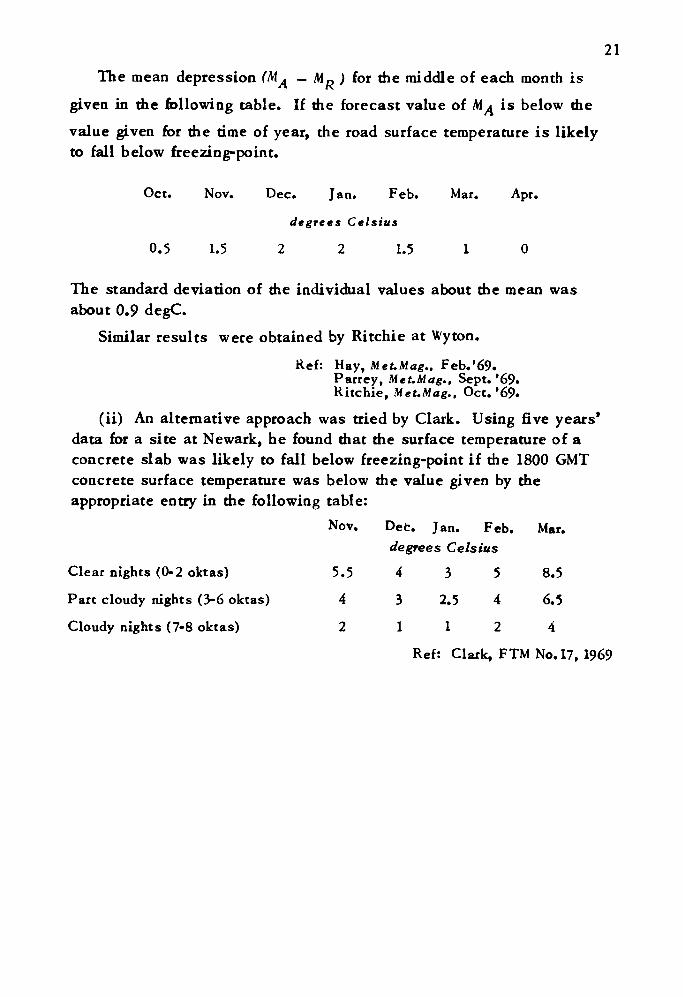
The mean depression (M^ — M R ) for the middle of each month is given in the following table. If the forecast value of M^ is below thevalue given for the dme of year, the road surface temperature is likely to fall below freezing-point.
Oct. Nov. Dec. Jan. Feb. Mar. Apr.
degrees Celsius
0.5 1.5 2 2 1.5 1 0
The standard deviation of the individual values about the mean was about 0.9 degC.
Similar results were obtained by Ritchie at Wyton.
Ref: Hay, Met.Mag.. Feb.'69.Parrey, MetMag., Sept.'69. Ritchie, Met.Mag., Oct.'69.
(ii) An alternative approach was tried by Clark. Using five years' data for a site at Newark, he found that the surface temperature of a concrete slab was likely to fall below freezing-point if the 1800 GMT concrete surface temperature was below the value given by the appropriate entry in the following table:
Nov. Det. Jan. Feb. Mar. degrees Celsius
Clear nights (0-2 oktas) 5.5 4 3 5 8.5
Part cloudy nights (3-6 oktas) 4 3 2.5 4 6.5
Cloudy nights (7-8 oktas) 21124
Ref: Clark, FTM No. 17, 1969
22
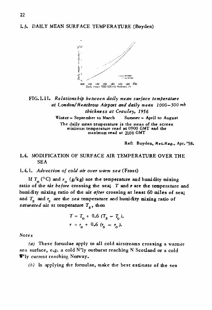
1.3. DAILY MEAN SURFACE TEMPERATURE (Boyden)
E
-= --'' ———winter Q ,~ ----summer
5000 5100 5200 SOT 5«6 5500 5600 5700 Daily mean 1000-500 mb thickness im 1
FIG. 1.11. Relationship between daily mean surface temperatureat London/Heathrow Airport and daily mean 1000-500 mb
thickness at Crawley, 1956 Winter = September to March Summer = April to August
The daily mean temperature is the mean of the screenminimum temperature read at 0900 GMT and the
maximum read at 2100 GMT
Ref: Boyden, M e t.Mag.. Apr. '58.
1.4. MODIFICATION OF SURFACE AIR TEMPERATURE OVER THESEA
1.4.1. Advection of cold air over warm sea (Frost)
If T (°C) and r (g/kg) are the temperature and humidity mixing ratio of the air before crossing the sea; T and r are the temperature and humidity mixing ratio of the air after crossing at least 60 miles of sea; and T and r are the sea temperature and humidity mixing ratio of saturated air at temperature TS , then
T= TQ + 0.6 (Ts - TQ ),
r = TQ + 0.6 (rs - rQ ).
Notes
(a) These formulae apply to all cold airstreams crossing a warmer sea surface, e.g. a cold N'ly outburst reaching N Scotland or a cold W'ly current reaching Norway.
(b) In applying the formulae, make die best estimate of the sea
23
surface temperature along the trajectory. Determine rQ and r from the tephigram.
Ref: HWF 14.10.1.Frost, SDTM N o. 19.
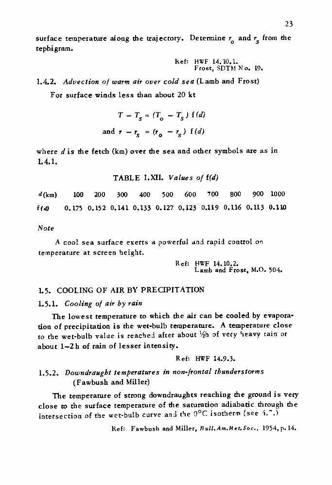
1.4.2. Advection of warm air over cold sea (Lamb and Frost)
For surface winds less than about 20 kt
and r -rs = (rQ - rg ) t(d)
where d is the fetch (km) over the sea and other symbols are as in 1.4.1.
TABLE l.XII. Values of f(d)
<f(km) 100 200 300 400 500 600 700 800 900 1000
f(4 0.175 0.152 0.141 0.133 0.127 0.123 0.119 0.116 0.113 0.110
Note
A cool sea surface exerts a powerful and rapid control on temperature at screen height.
Ref: HWF 14.10.2.Lamb and Frost, M.O. 504.
L5. COOLING OF AIR BY PRECIPITATION
1.5.1. Cooling of air by rain
The lowest temperature to which the air can be cooled by evapora tion of precipitation is the wet-bulb temperature. A temperature close to the wet-bulb value is reached after about V2h of very heavy rain or about 1— 2h of rain of lesser intensity.
Ref: HWF 14.9.3.
1.5.2. Downdraught temperatures in non-frontal thunderstorms (Fawbush and Miller)
The temperature of strong downdraughts reaching the ground is very close to the surface temperature of the saturation adiabatic through the intersection of the wet-bulb curve and the 0°C isotherm (see i."'.)
Ref: Fawbush and Miller, Bull.Am.Mct.Soc., 1954, p. 14.
24
1.5.3- Cooling of air by snow (Lumb)
Reduction of the surface temperature to O^C as a result of downward penetration of snow is unlikely
(i) in prolonged frontal precipitation if the wet-bulb temperature at the surface is higher than 2.5*C, and
(ii) within extensive areas of moderate or heavy instability precipi tation if the wet-bulb at the surface is higher than 3-5°C-
Note
The relation between wet-bulb temperatures and the form of precipi tation is given in 6.5.4. and 6.5-5.
Ref: Lumb, Met.Mag., Jan '63.
CHAPTER 2. FOG
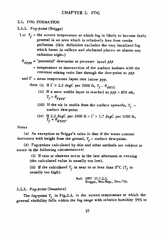
2.1. FOG FORMATION 2.1.1. Fog'point (Briggs)
Let T, = the screen temperature at which fog is likely to become fairly general in an area which is relatively free from smoke pollution (this definition excludes the very localized fog which forms in valleys and sheltered places on almost any radiation night.)
®dppp * 'potential' dew-point at pressure level ppp= temperature at intersection of the surface isobars with the
constant mixing ratio line through the dew-point at pppand F = mean temperature lapse rate below ppp.
then (i) If T > 2.2 degC per 1000 ft, Tf =- 0rf850(ii) If a more stable layer is reached at ppp > 850 mb,
(iii) If the air is stable from the surface upwards, T, = surface dew-point.
(iv) If 2.2 degC per 1000 f t > T > 1.7 degC per 1000 ft, Tf ' ̂ 900'
Notes(a) An exception to Briggs' s rules is that if the water content
increases with height from the ground, T, = surface dew-point.(b) Fog-points calculated by this and other methods are subject to
errors in the following circumstances:(i) If rain or showers occur in the late afternoon or evening
(the calculated value is usually too low).(ii) If the calculated T/ is near to or less than 0°C (T, is usually too high).
Ref: HWF 17.7.2.3.Briggs, Met.Mag., Dec.'50.
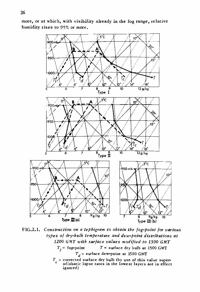
2.1.2. Fog-point (Saunders)The fog-point T, in Fig.2.1. is the screen temperature at which the
general visibility falls within the fog range with relative humidity 95% or
25
26
more, or at which, with visibility already in the fog range, relative humidity rises to 95% or more.
,'/ 4' / 6° / »8 9 10 Type I
12g/kg
7 8 Type HI (a)
7 8 9g/kg 10 Type IE (b)
FIG.2.1. Construction on a tephigram to obtain the log-point for various types of dry-bulb temperature and dew-point distributions at
1200 GMT with surface values modified to 1500 GMTT = surface dry bulb at 1500 GMT
T = surface dew-point at 1500 GMTT - corrected surface dry bulb (by use of this value super-
c adiabatic lapse rates in the lowest layers are in effect ignored)
T = fog-point
27(i) Select the 1200 GMT tephigrarn most representative of the air
which will be over the area during the night and redraw the temperature and dew-point curves to allow for changes taking place nc.ir the surface up to 1500 GMT (see Note (a)).
(ii) The heavier pecked lines of Fig.2.1. indicate constructions on the tephigram to determine T,. These depend on which of the following types of dew-point lapse is appropriate.
Type I — Constant dew-point lapse aloft; surface dew-point on, or to the right of, downward extension of upper dew-noint curve.
Type II — Dew-point lapse aloft increasing at high levels within the layer (up to level AB); surface dew-point as in Type I.
Type HI — Surface dew-point to the left of downward extension of upper dew-point curve;
(a) temperature lapse in lowest layer less than dry adiabatic,
(b) temperature lapse in lowest layer equal to, or greater than, dry adiabatic.
Notes
(a) Strictly the technique requires a tephigram for 1500 GMT, the time for routine radiosonde ascents when the technique was published.
(b) In extreme cases where a subsidence inversion has brought dry air down to only 20 or 30 mb above the ground, it is usually better to use the surface dew-point as the fog-point.
(c) See cautionary note (b) in 2.1.1.
Ref: HWF 17.7.2.2.Saunders, Met.Mag., Aug. '50.Saunders and Summersby, Met.Mag., Sept. '5 LSaunders, Met.Mag., Mar. '58.
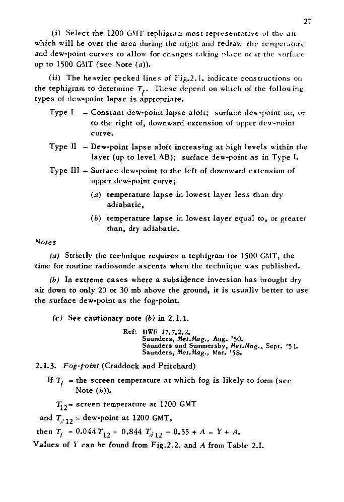
2.1.3. Fog-point (Craddock and Pritchard)
If T, = the screen temperature at which fog is likely to form (see Note (b)).
T12 = screen temperature at 1200 GMT and T,/12 = dew-point at 1200 GMT,
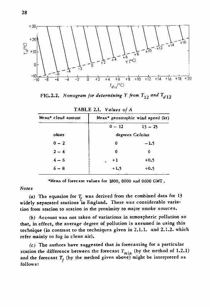
then Tf = 0.044 TU + 0.844 Td u - 0.55 -I- A = Y + A. Values of V can be found from Fig.2.2. and A from Table 2.1.
28
+30
-10 -8 -6 -4 -2 0 +2 +4 +6 +8 +10 +12 +14 +16 +18 +20
FIG.2.2. Nomogram for determining Y from T^ and
TABLE 2.1. Values of AMean* cloud amount
oktas
0-2
2-4
4-6
6-8
Mean* geostrophic wind speed (kt)
0-12 13-25
degrees Celsius
0 -1.5
0 0
+ 1 -fO.5
+ 1.5 +0.5
•Mean of forecast values for 1800, 0000 and 0600 GMT.
Notes(a) The equation for T. was derived from the combined data for 13
widely separated stations in England. There was considerable varia tion from station to station in the proximity to major smoke sources.
(b) Account was not taken of variations in atmospheric pollution so that, in effect, the average degree of pollution is assumed in using this technique (in contrast to the techniques given in 2.1.1. and 2.1.2. which refer mainly to fog in clean air).
(c) The authors have suggested that in forecasting for a particular station the difference between the forecast T - (by the method of 1.2.1) and the forecast T/ (by the method given above) might be interpreted as follows:
29
T,- T ./ mm
-t- 1 degC or higher
+ 0.5 degC to -1.5 degC
—2 degC or lower
Forecast
Fog
More or less serious risk of fog
Negligible risk of fog
Ref: H\X'F 17.7.2.1.Craddock and Pritchard, MRP 624.
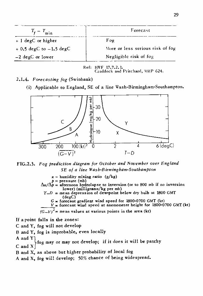
2.1.4. Forecasting fog (Swinbank)
(i) Applicable to England, SE of a line Wash-Birmingham-Southampton.
6(degC)(G-V T-D
FIG.2.3. Fog prediction diagram for October and November over EnglandSE of a line Wash-Birmingham-Southampton
x = humidity mixing ratio (g/kg) p = pressure (mb)
Ajr/Ap = afternoon hydrolapse to inversion (or to 800 mb if no inversionlower) (milligrams/kg per mb)
T—D = mean depression of dew-point below dry bulb at 1800 GMT(degC)
G = forecast gradient wind speed for 1800-0700 GMT (kt) ___V «: forecast wind speed at anemometer height for 1800-0700 GMT(kt)
If a point C and Y, B and Y, A and Y]
C and XJ B and X, A and X,
(G—V) = mean values at various points in the area (kt)
falls in the zones:fog will not developfog is improbable, even locally
fog may or may not develop; if it does it will be patchy
as above but higher probability of local fogfog will develop; 50% chance of being widespread.
31
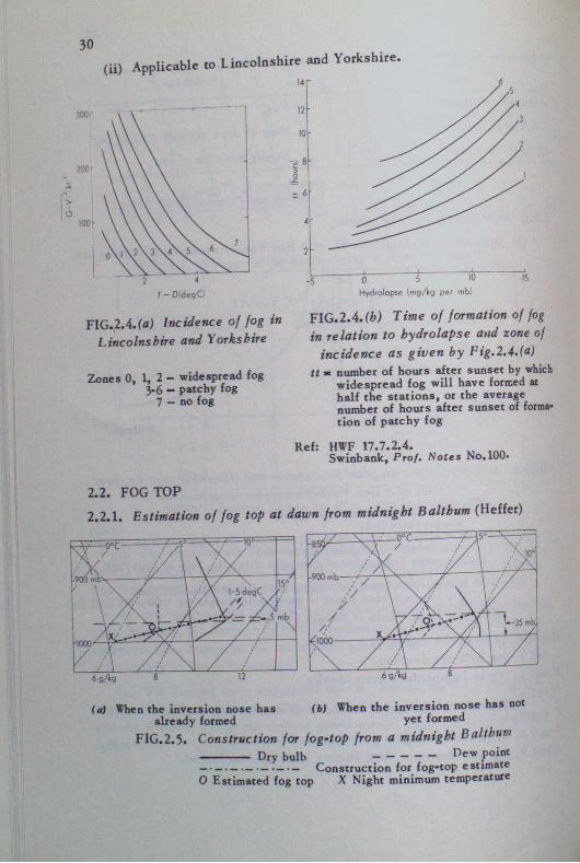
(i) If the nose has already formed on the temperature curve, the level is raised by 5 mb and the temperature is decreased by 1.5 degC and this point is joined to the night minimum temperature by a straight line on the tephigram. The point where this line and the dew-point curve inter sect (Oin Fig.2.5.fc.)) represents the fog top at dawn.
(ii) If a nose has not yet formed on the temperature curve at mid- night, the point 35 mb above the ground is joined to the night minimum surface temperature and the fog-point at dawn estimated as before (O in Fig. 2.5. (6)).
Ref: Heffer, Met.Mag.. Sept.'65.
2.3. FOG CLEARANCE BY INSOLATION
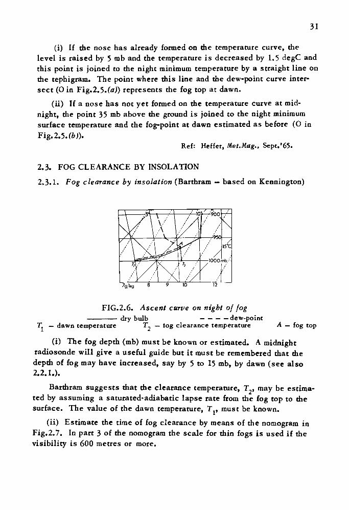
2.3.1. Fog clearance by insolation (Barthram — based on Kennington)
7g/kg 8 9 10
FIG.2.6. Ascent curve on night of fog—————— dry bulb — — — — dew-point
T — dawn temperature T. — tog clearance temperature A — fog top
(i) The fog depth (mb) must be known or estimated. A midnight radiosonde will give a useful guide but it must be remembered that the depth of fog may have increased, say by 5 to 15 mb, by dawn (see also 2.2.1.).
Barthram suggests that the clearance temperature, T2, may be estima ted by assuming a saturated-adiabatic lapse rate from the fog top to the surface. The value of the dawn temperature, Tj, must be known.
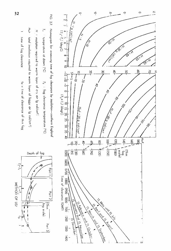
(ii) Estimate the time of fog clearance by means of the nomogram in Fig.2.7. In part 3 of the nomogram the scale for thin fogs is used if the visibility is 600 metres or more.
12
34
56
7
(T2-T
,1 (degC
)9
10 -15 -10
-5 0
5 10
15 20
25 30
35 40
(r,+ r,) (degC
)0500
0600 0700
0800 0900
1000 1100
1200 Tim
e of clearance (GM
T)1300
1400
FIG.
2.7. N
omogram
for assessing fim
e of fog clearance by insolation—southern E
ngland
T, -
temperature at daw
n (°C)
T2 = fog
clearance temperature (°C
)
H -
insolation required to warm
layer of dry air (g cal/cm
2 )
HxF -
total insolation
required to warm
layer of foggy air (g
cal/cm2)
t tim
e of fog
clearance 'a
= tim
e of clearance of thin fog
a0)a
Part 1
Part 2
h-^<<sc4-
(Thmfog
scale)Part 3
ME
THO
D O
F USE
33Notes
(a) The assumed values of available heat are those appropriate to southern England. For northern parts of the British Isles the corre'spond- ing values are less and consequently fog is likely to clear later than would be estimated from Fig.2.7. — especially during winter.
(b) Heffer has tested this technique for 8 stations in East Anglia and the E Midlands.
Ref: Kennington, Met.Mag., Mar. '61. Barthram, Met.Mag., Feb.'64. Heffer, Met.Hag., Sept.'65.
2.3.2. Fog clearance by insolation (Jefferson)(i) Estimate the fog top either from examination of a representative
tephigram or from any available reports (allowing for possible upward extension of fog due to increased turbulence around dawn).
(ii) The clearance temperature, T , is estimated in Jefferson's method on the assumption of a dry adiabatic from surface to fog top.
(iii) Estimate the temperature rise by the method given in 1.2.Ref: HWF 17.8.
Jefferson, Met.Mag., Apr.'50.
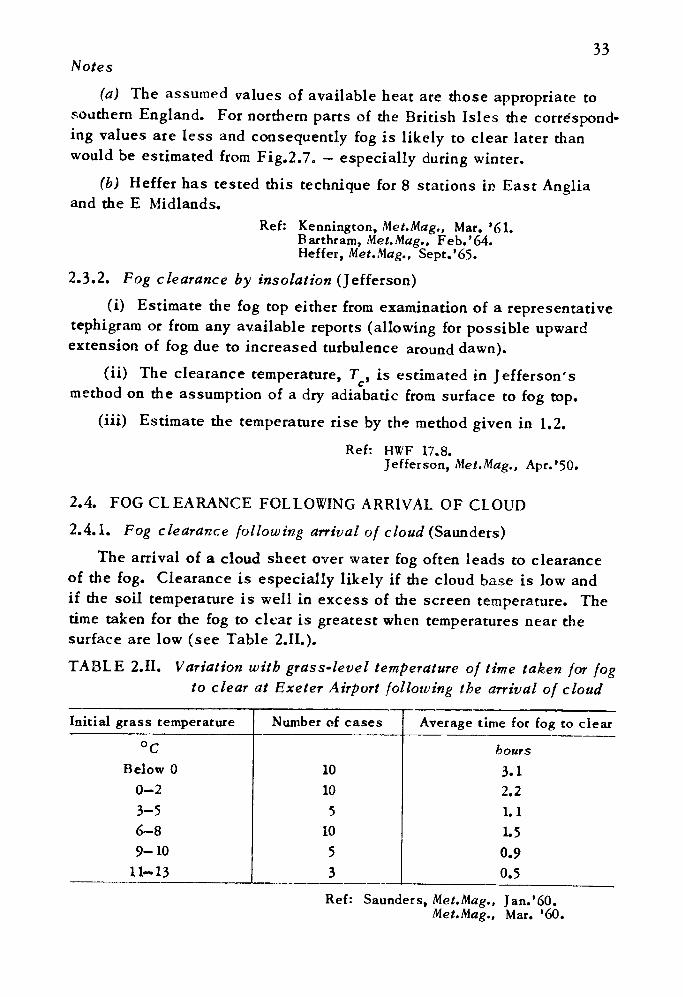
2.4. FOG CLEARANCE FOLLOWING ARRIVAL OF CLOUD 2.4.1. Fog clearance following arrival of cloud (Saunders)
The arrival of a cloud sheet over water fog often leads to clearance of the fog. Clearance is especially likely if the cloud base is low and if the soil temperature is well in excess of the screen temperature. The time taken for the fog to clear is greatest when temperatures near the surface are low (see Table 2.II.).TABLE 2.II. Variation with grass-level temperature of time taken for fog
to clear at Exeter Airport following the arrival of cloud
Initial grass temperature°C
Below 00-23-56-89-10
11-13
Number of cases
1010
51053
Average time for fog to clear
hours3.12.21.11.50.90.5
Ref: Saunders, Met.Mag., Jan.'60. Met.Mag.. Mar. '60.
34
2.5. ADVECTION FOGConditions for formation are:
(i) Original dew-point of the air higher than die temperature of the underlying surface.
(ii) A stable lapse rate of temperature and only a slight hydrolapse.
(iii) A suitable wind in the first instance to transport the air from die warm surface to a colder surface.
2.5.1. Sea fog
(i) Two important cases of die formation of advection fog over the sea occur in air streams approaching the British Isles from the SW and from the E (over the North Sea). An estimate of the cooling of air crossing the North Sea can be made by the method given in 1.4.2.
(ii) Sea fogs when surface winds are as strong as 25 kt are not uncommon.
(iii) Occasionally fog which has been lying over the sea may be brought across the coast — even at the time of maximum insolation — by a sea-breeze.
2.5.2. Advection fog over the land(i) For advection fog over the land to be at all widespread or persis
tent the ground must be very cold — either frozen or snow covered.(ii) Advection fog is unlikely over the land if the surface wind
exceeds about 10 kt.
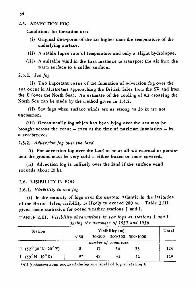
2.6. VISIBILITY IN FOG
2.6.1. Visibility in sea fog(i) In the majority of fogs over the eastern Atlantic in the latitudes
of the British Isles, visibility is likely to exceed 200 m. Table 2.III. gives some statistics for ocean weather stations J and I.
TABLE 2.III. Visibility observations in sea fogs at stations J and Iduring the summers of 1957 and 1958
Station
J (52°30'N 20°W)
I (59°N 19°W)
<50
09*
Visibility (m)50-200 200-500
number of occasions15 56
48 31
500- 1000
5331
Total
124
119
*A11 9 observations occurred during one spell of fog at station I.
35
(ii) There is some evidence that visibilities are lower in sea fogs in more northern (and cooler) waters.
(iii) When sea fogs form as a moist land-breeze crosses the coast to an adjacent cold sea and there is marked rapid cooling below the dew- point (for example North Sea fogs in early summer), very dense fog may be quickly formed.
Ref: HWF 17.10.1. 2.6.2. Visibility in radiation fog
(i) In country districts rapid thickening of radiation fog after its formation is probably typical. For instance, at Exeter Airport and at Merryfield the deterioration of visibility from 1000 m to 200 m or less occurs within 1 h in about 1A of the fogs and within 2 h in about % of the fogs.
(ii) In districts where rhere is heavy smoke pollution which is several hundred feet thick vertically, such sudden deteriorations may be less common. The increase in smoke concentration may reduce visibility to below 1000 m long before the temperature has reached the fog-point. There is also some evidence that the subsequent fall of visibility as condensation takes place is also more gradual than in 'clean' air.
Ref: HWF 17.10.2.Saunders, Met.Mag., Jan.'60.
Met.Mag., Dec.'57.
CHAPTER 3. CLOUD
3.1. STABILITY DEFINITIONSStatic stability (or hydrostatic stability or vertical stability) in a
layer of air is normally assessed by its influence on a parcel of its air which is made to move vertically through the layer. The state of the layer of air is then defined as follows:
Stable: the buoyancy force opposes the movementUnstable: the buoyancy force assists the movementNeutral: die buoyancy force is zero.
Latent instability. If the buoyancy force opposes upward motion initially but assists it when the parcel of air reaches a higher level, the whole layer of air is said to possess latent instability.
The buoyancy of a parcel of air depends on its temperature relative to the temperature of the air around it. The parcel of air, if it is cloudy, acquires a temperature in moving vertically which depends partly on release or absorption of latent heat. Thus the stability of a layer of air depends on its humidity. The following terms are used to describe the stability of a layer of air in relation to both temperature and humidity:
Absolute stability: stable regardless of its humidity ( y < TS )
Absolute instability: unstable regardless of its humidity(y>r^, i.e. a superadiabatic lapse rate)
Conditional instability: stable if unsaturated, unstable ifsaturated (T^>y>T ).
Potential instability (or convective instability). If a column of air is lifted bodily the temperature decrease varies from level to level, particularly because some layers become cloudy (and acquire the released latent heat) sooner than others. Thus certain layers become unstable. The layers which are thus potentially unstable are those in which the potential wet-bulb temperature decreases with height.
36
37
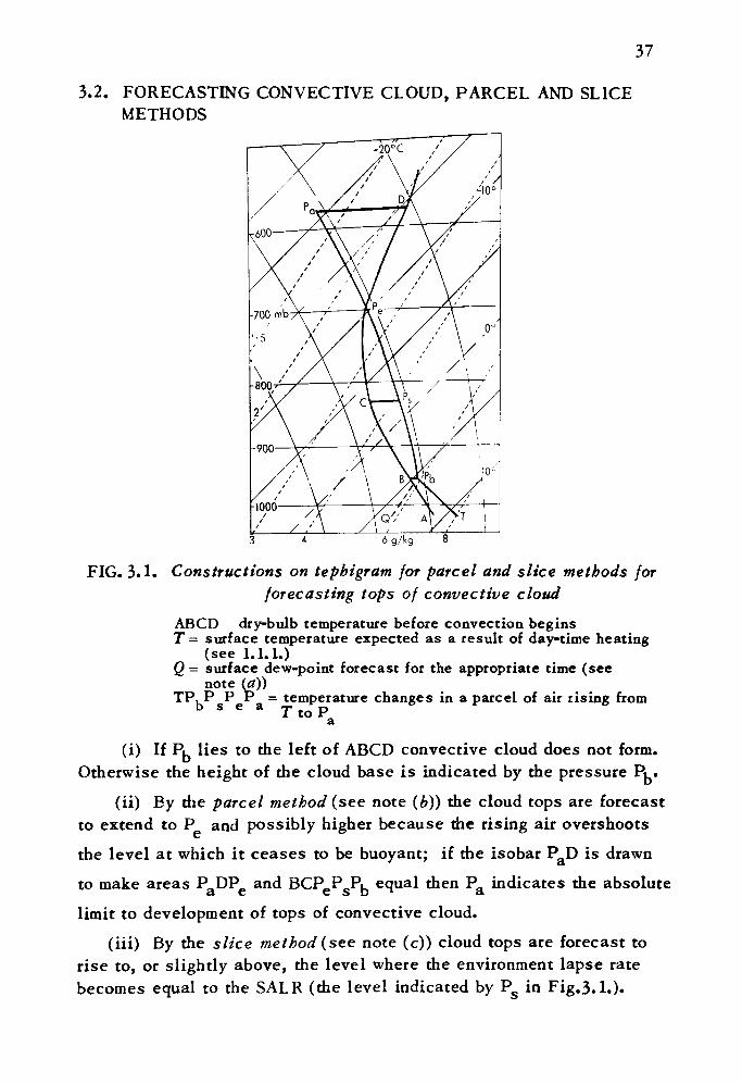
3.2. FORECASTING CONVECTIVE CLOUD, PARCEL AND SLICE METHODS
6gAg
FIG. 3.1. Constructions on tephigram for parcel and slice methods forforecasting tops of convective cloud
ABCD dry-bulb temperature before convection beginsT= surface temperature expected as a result of daytime heating
(see 1.1.1.) Q = surface dew-point forecast for the appropriate time (see
note (a)) TP, P P P = temperature changes in a parcel of air rising from
b s e a TtoPa
(i) If Pjj lies to the left of ABCD convective cloud does not form. Otherwise the height of the cloud base is indicated by the pressure P^.
(ii) By die parcel method (see note (b)) the cloud tops are forecast to extend to P and possibly higher because the rising air overshoots
the level at which it ceases to be buoyant; if the isobar P&D is drawn
to make areas P,DP^ and BCP-P^Pi equal then P0 indicates the absoluteci c C S D **
limit to development of tops of convective cloud.
(iii) By the slice method (see note (c)) cloud tops are forecast to rise to, or slightly above, the level where the environment lapse rate becomes equal to the SALR (the level indicated by Pg in Fig.3. !.)•
38 Notes
(a) The surface dew-point is subject to diurnal variation. An esti mate of the value to be expected during convection can be made from the preceding midnight ascent by extrapolating to the surface level the dew-points in the layer some 50-100 mb above the surface.
(b) The parcel method depends on the simplifying assumptions that:
(1) the rising parcels of air do not cause compensating downward motion, and therefore adiabatic warming of the environmental air, and(2) mixing of air does not occur between the parcels and the environment.
(c) The slice method is an attempt to allow for the compensatory downward motion and warming of the environment. Some relationships between cloud levels observed and those forecast by the parcel and slice methods are given in 3.3. and 3.4.
Ref: HWF 3.6.1., 3.6.2., 16.6.5.Petterssen et alii, Geofys. Publr, Oslo,
16, No. 10, 1945.
3.3. BASE OF CONVECTIVE CLOUD (Petterssen et alii)
For a convective cloud which does not give precipitation the pressure at the base can be estimated as 25 mb less than the condensation pressure (Pi in Fig.3.1.) computed from the accompanying temperature and dew-point at the surface (i.e. the cloud base is estimated to be about 700 ft higher than the computed condensation level). On 75% of occasions the actual pressure at the cloud base is within 25 mb of this estimate.
Notes(a) This relationship was derived from aircraft ascents made at
Aldergrove and Bircham Newton (Norfolk) during the months April to September.
(b) In an investigation into the diurnal variation of small shower clouds over Bedfordshire during several days in August, Browne, Day and Ludlam found a similar relationship between the cloud base and computed condensation level up to the time of maximum temperature; afterwards the cloud base remained at approximately the same height or fell only a few hundred feet although the computed condensation
39
level fell rapidly until it was about 3000 ft below cloud base.
Ref: HWF 16.6.5.1.Petterssen d alii, C.eofys. Puhlr, Oslo,
16, No. 10, 1945. Browne, Day and Ludlam, Met.Mag., Mar. '55.
3.4. TOPS OF CONVECTIVE CLOUDRelationships found by various investigators between the forecast
heights of convective cloud tops by the parcel or slice methods and observed heights are not altogether consistent. On the whole reports suggest that
(i) convective cloud tops mainly reach levels between P and P (Fig.3.1.), and
(ii) with large convective storms — particularly storms which are sustained by a favourable wind field on the synoptic scale and are extensive horizontally — some cloud tops may reach Pa (Fig.3.1.)« Cloud tops associated with large storms have been reported to extend as high as 20 000 ft above the tropopause (see 6.4.8.).
Ref: HWF 16.6.5.2.Petterssen et alii, Geofys. Publr,
Oslo, 16, No. 10, 1945. Roach, Aero. Res. Coun.
28044, 1966. Ludlam and Scorer, Q.Jnl R. Met.
Soc., 1953, p.317.
3.5. FORMATION OF STRATUS BY NOCTURNAL COOLING
3.5.1. Temperature at which stratus forms (Saunders)
(i) Obtain the fog-point. T/,by the method of 2.1.1.
(ii) Assess the height of the top of surface turbulence at night (e.g. by the method of 3.5.2.).
(iii) On a tephigram draw the constant mixing ratio line through T, (plotted on the surface isobar).
(iv) From the intersection of this line with the isobar correspond ing to the top of the surface turbulent layer draw a dry adiabatic. The intersection of the adiabatic with the surface isobar indicates the temperature at which stratus will form.
Ref: HWF 16.6.3.
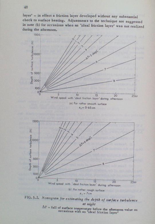
3.5.2. Depth of surface turbulence at night (Gifford)
This technique gives an estimate of the height of the top of surface turbulence following an afternoon when there was an 'ideal friction
41
The nomograms given in Fig.3.2. are for a latitude of 53° (the varia tions of latitude within the U.K. make only a slight difference to the results) and for an anemometer height of 10 metres (the height above open level terrain for standard exposure).
An estimate has to be made of z , a parameter of surface roughness, which can vary from place to place and from sector to sector at a given place according to the average height of upwind obstructions. The values of z_ for which the nomograms are given can be considered fairly extreme: 0.65 cm is the sort of value appropriate to flow off a rather smooth surface (e.g. the sea) and 7 cm to flow off a rather rough surface (e.g. a city).
Notes
(a) This technique has been shown to be suitable for several aero dromes in the U.S.A. The technique has not been tested in the U.K.
(b) After a day on which an 'ideal friction layer* is not realized (because of low cloud cover or precipitation preventing normal heating) the depth of turbulence at night is restricted and stratus can be expected to develop on average at only half the height shown by the appropriate nomogram.
(c) The technique implies that with a fall of surface temperature of about 9 degC or more from the afternoon value at the time of the 'ideal friction layer', stratus will form (humidity being favourable) at the surface regardless of the afternoon wind speed.
Ref: Gifford, Bull. Am.Met. Soc., 1950, p.31.
3.6. SPREAD OF STRATUS FROM THE NORTH SEA ACROSS EAST ANGLIA (Sparks)
When winds are off the North Sea and stratus covers the sea but has dispersed over land on account of day-time heating, then the inland spread of stratus during the evening and night can be forecast as follows:
(i) In the absence of a suitable temperature sounding through thestratus, the temperature at which the stratus cleared in the morning provides the best estimate of the temperature at the coast when stratus will start to move inland.
(ii) The movement of stratus inland can be forecast from the directions and speeds of surface winds at a time when convection and turbu lence are still operative in the lowest layers (say 1800 GMT in summer). This is likely to give a better forecast than one based
42
on the pattern of isobars, particularly if there is sharp anticy- clonic curvature.
(iii) Stratus may form over high ground before the arrival of the main cloud sheet forecast as in 3.5.1.
Ref: Sparks, Met.Mag.. Dec. '62.
3.7. DISPERSAL OF STRATUS BY INSOLATIONIt is assumed that the cloud will clear when the surface temperature
reaches such a value as to establish a dry-adiabatic lapse rate up to the level of the stratus top. The time taken to attain this temperature can be assessed by the method of 1.1.2.
Ref: HWF 16.6.3.2.
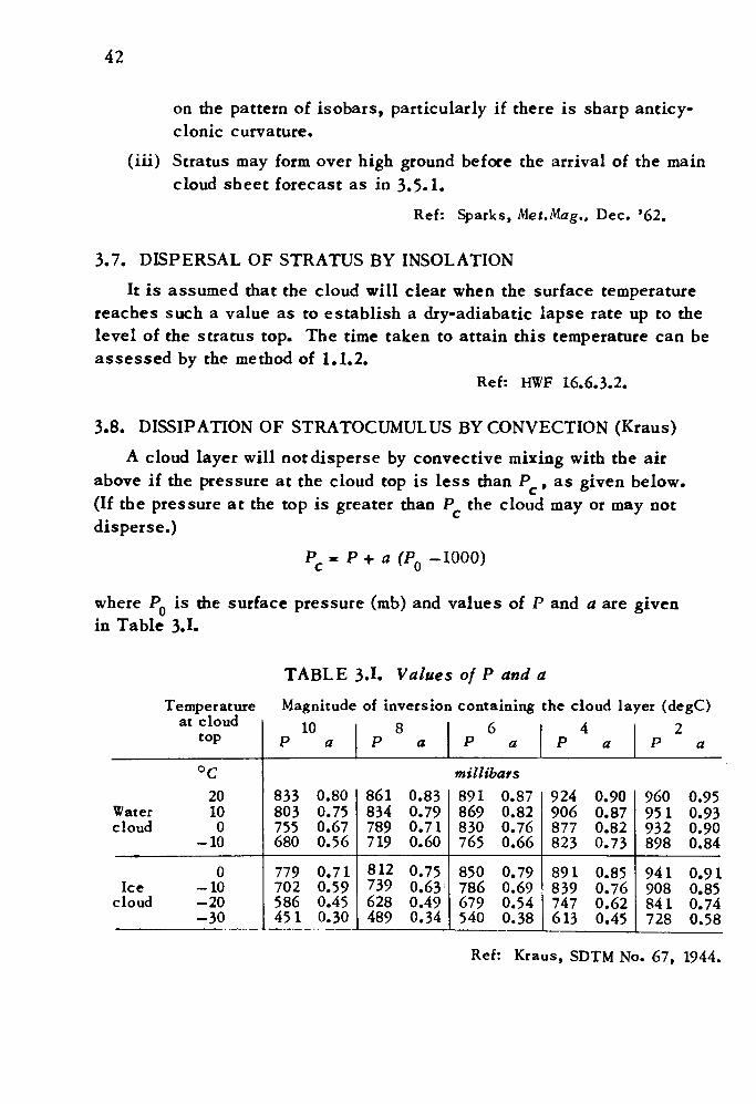
3.8. DISSIPATION OF STRATOCUMULUS BY CONVECTION (Kraus)A cloud layer will not disperse by convective mixing with the air
above if the pressure at the cloud top is less than P , as given below. (If the pressure at the top is greater than P the cloud may or may not disperse.)
Pc - P + a (PQ -1000)
where PQ is the surface pressure (mb) and values of P and a are given in Table 3.1.
TABLE 3.1. Values of P and a
Temperature Magnitude of inversion containing the cloud layer (degC)at cloud
top
°C
20 Water 10 cloud 0
-10
0 Ice - 10
cloud -20 -30
10 P a
833 0.80 803 0.75 755 0.67 680 0.56
779 0.71 702 0.59 586 0.45 451 0.30
8 P a
861 0.83 834 0.79 789 0.71 719 0.60812 0.75 739 0.63 628 0.49 489 0.34
6 P a
millibars891 0.87 869 0.82 830 0.76 765 0.66
850 0.79 786 0.69 679 0.54 540 0.38
4 P a
924 0.90 906 0.87 877 0.82 823 0.73
891 0.85 839 0.76 747 0.62 613 0.45
2 P a
960 0.95 95 1 0.93 932 0.90 898 0.84
941 0.91 908 0.85 841 0.74 728 0.58
Ref: Kraus, SDTM No. 67, 1944.
4 7-
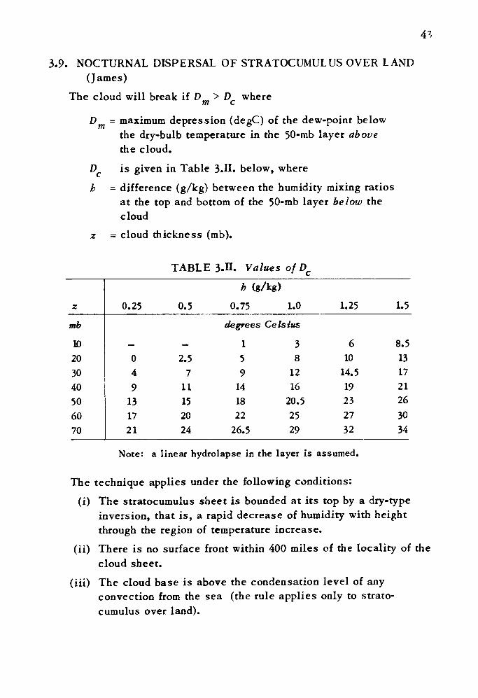
3.9. NOCTURNAL DISPERSAL OF STRATOCUMULUS OVER LAND (James)
The cloud will break if D > D wherem c
D = maximum depression (degC) of the dew-point below the dry-bulb temperature in the 50-mb layer above the cloud.
D is given in Table 3.H. below, where
h = difference (g/kg) between the humidity mixing ratios at the top and bottom of the 50-mb layer below the cloud
z = cloud thickness (mb).
TABLE 3.H. Values of DC
z
mb
10203040506070
0.25 0.5
b (g/kg)
0.75 1.0 1.25 1.5
degrees Celsius
—049
131721
—2.5
711152024
159
141822
26.5
38
1216
20.52529
610
14.519232732
8.5131721263034
Note: a linear hydrolapse in the layer is assumed.
The technique applies under the following conditions:
(i) The stratocumulus sheet is bounded at its top by a dry-type inversion, that is, a rapid decrease of humidity with height through the region of temperature increase.
(ii) There is no surface front within 400 miles of the locality of the cloud sheet.
(iii) The cloud base is above the condensation level of any convection from the sea (the rule applies only to strato cumulus over land).
44
(iv) The cloud sheet is extensive, covering several hundred square miles, and gives almost complete cloud cover, more than 6/8 for at least 2 consecutive hours. (The cloud was regarded as having dissipated if it broke to 2/8 or less for at least 2 consecutive hours.)
Failures of the technique in day-to-day forecasting can often be attributed to
(i) inaccurate assessment of the cloud thickness (in the absence of reports from aircraft), and
(ii) uncertainties as to the magnitude and steepness of the tempera ture inversion and hydrolapse, because of the lag of radiosonde elements.
Ref: HWF 16.6.3.4.James, Met.Mag., July '56.
Q.Jnl R. Met. Soc.. 1959, P. 120.
3.10. FORECASTING CIRRUS OVER THE BRITISH 1ST PS
3.10.1. Forecasting cirrus (James)
(i) Occurrence 6-9 b ahead
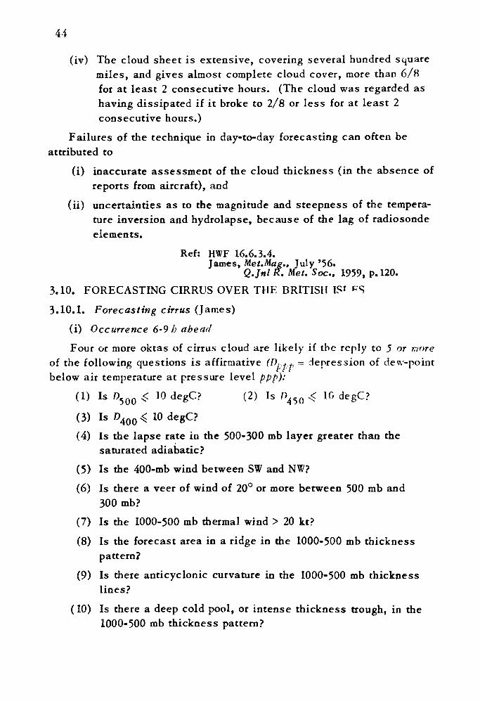
Four or more oktas of cirrus cloud are likely if the reply to 5 or more of the following questions is affirmative (V^t p = depression of dew-point below air temperature at pressure level ppp):
(1) Is D50Q ^ 10 degC? (2) Is P450 ^ 10 degC?
(3) IsD4 < lOdegC?
(4) Is the lapse rate in the 500-300 mb layer greater than the saturated adiabatic?
(5) Is the 400-mb wind between SW and NW?
(6) Is there a veer of wind of 20° or more between 500 mb and 300 mb?
(7) Is the 1000-500 mb thermal wind > 20 kt?
(8) Is the forecast area in a ridge in the 1000-500 mb thickness pattern?
(9) Is there anticyclonic curvature in the 1000-500 mb thickness lines?
(10) Is there a deep cold pool, or intense thickness trough, in the 1000-500 mb thickness pattern?
(11) Is the forecast area in, or just to the rear of, a ridge in the 300-mb contour pattern?
(12) Is the forecast area on the anticyclonic side of a 300-mb jet stream and within 300 miles of the jet axis?
(13) Is the forecast area up to 300 miles ahead of a surface warm front or occlusion?
(ii) Occurrence 24—3bh ahead
Four or more oktas of cirrus cloud are likely to occur if the reply to 2 or more of the following questions is affirmative:
(1) In the air which will be over the area during the forecast period, is the present dew-point depression at 500 mb or higher levels <; 10 degC (trace back the air using the 500-mb forecast chart)?
(2) Will the area be up to 300 miles ahead of a surface warm front or occlusion (use the surface forecast chart)?
(3) Will the area be on the anticyclonic side of a 300-mb jet stream and within 300 miles of the jet axis?
(4) Will the area be in, or just to the rear of, a 300-mb ridge?
(5) Will the area be in a thermal ridge (use 1000-500 mb pre-thickness chart)?
(6) Will the veer of wind between 500 mb and 300 mb be 20° or more?
Ref: HWF 16.6.4.1.James, Pro/. Notes No. 123, 1957.
3.10.2. Forecasting cirrus 6—12h ahead (Singleton and Wales-Smith)
The method given in 3.10.1. has been simplified and adapted to give some indication of the high-cloud cover to be expected. A score of 0, Yi or 1 is given for each gf the following questions according to whether the answer is 'no', 'uncertain' or 'yes* respectively:
(1) Is the forecast area in,or just to the rear of, a ridge in the 200-mb contour pattern?
(2) Is the forecast area on the anticyclonic side of a 200-mb jet stream and within 300 miles of the jet axis?
(3) Is the forecast area up to 300 miles ahead of a surface warm front or occlusion?
46The scores are added. Cirrus amounts are roughly associated asfollows:
Total score 0 V2 I lV2 2* 2l/2 3
Amount (oktas) 0123 4 56-7
*For a score of two the scatter of cloud amount values is particularly large so use of the fuller method of 3.10.1. is recommended to decide whether or not the amount will be at least 4 oktas.
Note
This technique is not likely to be adequate for forecasting cirrus produced by convection.
Ref: Singleton and Wales-Smith, Met.Mag., Apr. '60.
3.11. FORECASTING CIRRUS FORMED BY CONVECTION (Gayikian)(i) If straight or anticyclonic flow exists at 300-200 mb over the
area downstream from a thunderstorm area, cirrus may appear the next day and advance ahead of the ridge-line.
(ii) If the contours over the area downstream from the thunderstorm area are cyclonically curved, cirrus may or may not appear. It is most likely to appear if the flow is weak.
Ref: Gayikian, Forecasting manual for SAC operations, Offut, 1955, p. 194.
3.12. CIRRUS ASSOCIATED WITH THE JET STREAM
3.12.1. Cirrus associated with the jet stream (Sawyer and Ilett)
(i) Cirrus is considerably more frequent and extensive to the right of the jet stream than to the left.
(ii) The frontal and layer types of cirrus (and medium clouds) are more common to the right of the jet stream; anvil cirrus (and altocumulus from the spreading out of cumulus) is more common to the left.
(iii) When a well-defined boundary to frontal cirrus occurs the axis of the jet stream is often close to the boundary.
Ref: Sawyer and Ilett, Met.Mag., Oct. '51.
3.12.2. Cirrus associated with the jet stream (Frost)
From a pilot's point of view the main features consist of cirrus streamers with long tufted streaks and complex shear lines; the bands of cloud lie along the jet, sometimes for great distances together with
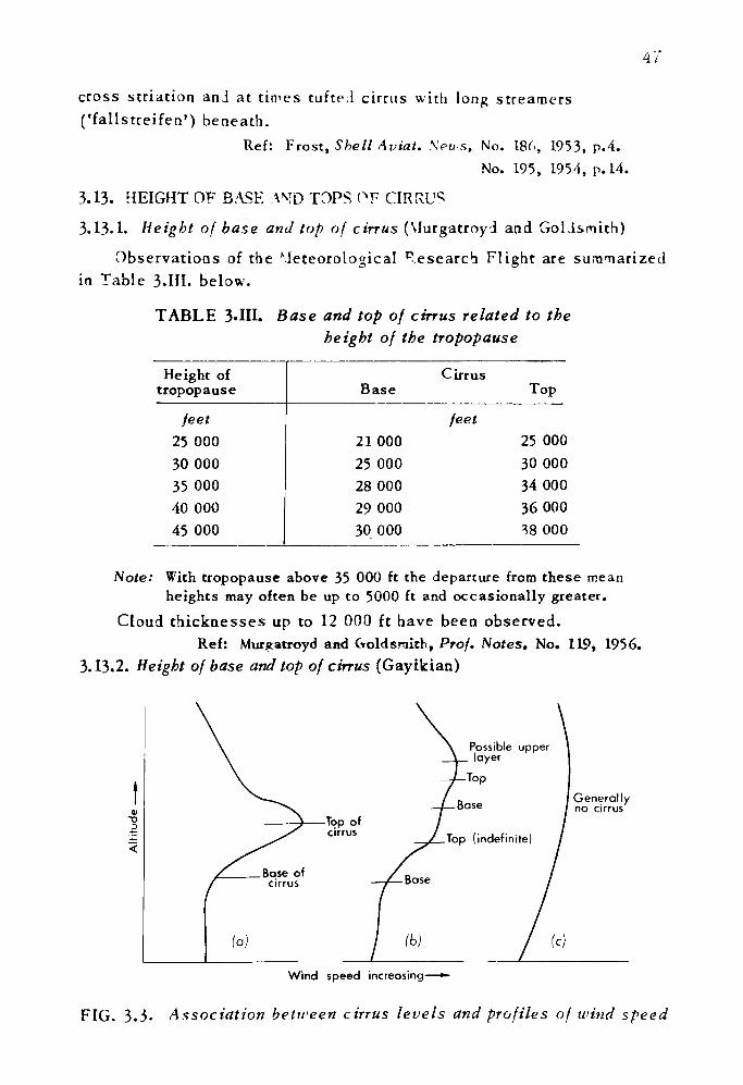
cross striation and at times tufted cirrus with long streamers ('fallstreifen') beneatli.
Ref: Frost, Shell Aviat. \ews. No. 186, 1953, p.4.No. 195, 1954, p. 14.
3.13. HEIGHT OF BASE A^D TOPS OF CIRRUS
3.13-1. Height of base and top of cirrus (Vlurgatroyd and Goldsmith)
Observations of the Meteorological Research Flight are summarized in Table 3.HI. below.
TABLE 3«HI. Base and top of cirrus related to theheight of the tropopause
Height of tropopause
feet25 0003000035 00040 00045 000
Base
2100025 0002800029 00030 000
Cirrus Top
feet25 00030 00034 0003600038 000
Note: With tropopause above 35 000 ft the departure from these mean heights may often be up to 5000 ft and occasionally greater.
Cloud thicknesses up to 12 000 ft have been observed.Ref: Murgatroyd and Goldsmith, Prof. Notes, No. 119, 1956.
3.13.2. Height of base and top of cirrus (Gaytkian)
Possible upper layer
•Top of cirrus
Generally no cirrus
Top (indefinite)
(b)
Wind speed increasing—*•
FIG. 3.3- Association between cirrus levels and profiles of wind speed
48
The presence and density of cirrus is related to variations of wind speed with height at the appropriate levels, as shown in Fig.3-3. Occurrence of cirrus is favoured and the cirrus is likely to be dense in a layer through which the wind increases rapidly with height, as inf ig.3.3.ffl). Uith a wind-speed profile such as that of Fig. 3.3.^) cirrus is likely to be of low density and in layers ti.rough a ^reut depth.
Ref: Gayikian, Forecasting manual for SAC operations, Offut, 1955, p. 194.
3.14. THE LOWERING OF CLOUD BASE DURING CONTINUOUS RAIN (Goldm-n)
(i) The base of a cloud layer will be at a height where the temper ature lapse changes from positive to less positive or to negative.
(ii) The base of a cloud layer will be at a height where the wet- bulb or dew-point depression is a minimum.
(iii) If the rain is of sufficient duration a ceiling (see note (a)) will occur below 2000 ft. Most frequently it is a ceiling below 800 ft.
(iv) During continuous rain a ceiling generally does not occur at the height of temperature discontinuity and/or maximum humidity until after the occurrence of a ceiling corresponding to the next higher level of temperature discontinuity and/or maximum humidity.
(v) The ceiling remains practically constant until the next lower cloud layer appears and increases in amount sufficiently for its base to become the ceiling.
Notes
(a) The ceiling is the height above the ground of the base of the lowest cloud layer covering more than half the sky.
(b) This technique was devised for places in the U.S.A. and has not been tested in the U.K.
Ref: HWF 16.6.2.2.Goldman, Mon. Weatb. Rev., Washington,
195 1, p. 133.
CHAPTER 4. WINDS
4.1. GEOSTROPHIC WINDS
Though the value of the geostrophic wind is often used as an approxi mation to the value of the actual wind, steady geostrophic flow occurs only when:
(i) the isobars (or contours) are straight, parallel and not changingwith time,(ii) there is no vertical motion, and
(iii) there are no external forces, e.g. friction.
Geostrophic scales for use with isobars on a constant-level chart (unlike those for contours on an isobaric chart) apply strictly for only one value of air density. With the Meteorological Office scales for surface charts, the correction required over the British Isles for depart ure from the assumed density exceeds 5% of the indicated speed only in exceptional conditions (i.e. with very low temperature and high pressure or with very high temperature and low pressure).
4.2. AGEOSTROPHIC EFFECTSThe ageostrophic wind (i.e. the vector difference between the actual
wind and the geostrophic wind) can be expressed mathematically as the sum of five terms (see Appendix 1.7.). One of these terms is due to ageo strophic acceleration and it is not possible to deal with this; the effect is t however, probably negligible inmost cases. The remaining four terms are due to:
(i) Friction. This term is important for surface winds but negligible for winds at upper levels. The effects of friction can be allowed for in forecasting surface wind by using statistical relationships such as those given in 4.4.
(ii) Vertical motion. This term is negligible both near the surface and near the maximum-wind level, but may reach about 5 kt in areas of strong vertical wind shear above and below the level of the jet core. The vector is directed towards the axis above and below jet entrances and away from the axis above and below jet exits. This term therefore acts in opposition to the cross-isobar component of the advective term (see (iv) below) on the cold side of a jet but in the same sense on the warm side.
49
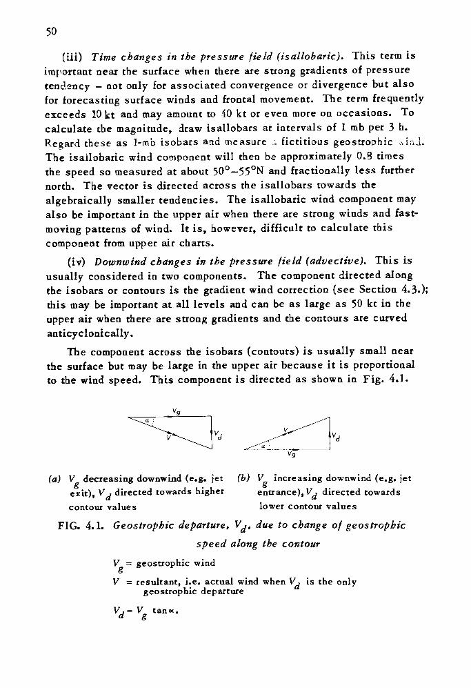
50
(iii) Time changes in the pressure field (isailobaric). This term is important near the surface when there are strong gradients of pressure tendency - not only for associated convergence or divergence but also for forecasting surface winds and frontal movement. The term frequently exceeds 10 kt and may amount to 40 kt or even more on occasions. To calculate the magnitude, draw isallobars at intervals of 1 mb per 3 h. Regard these as 1-mb isobars and measure u fictitious geostrophic v. i.ij. The isailobaric wind component will then be approximately 0.8 times the speed so measured at about 50°—55°N and fractionally less further north. The vector is directed across the isallobars towards the algebraically smaller tendencies. The isailobaric wind component may also be important in the upper air when there are strong winds and fast- moving patterns of wind. It is, however, difficult to calculate this component from upper air charts.
(iv) Downwind changes in the pressure field (advective). This is usually considered in two components. The component directed along the isobars or contours is the gradient wind correction (see Section 4.3.); this may be important at all levels and can be as large as 50 kt in the upper air when there are strong gradients and the contours are curved anticyclonically.
The component across the isobars (contours) is usually small near the surface but may be large in the upper air because it is proportional to the wind speed. This component is directed as shown in Fig. 4.1.
(a) V decreasing downwind (e.g. jet (b) V increasing downwind (e.g. jetentrance), V, directed towards lower contour values
exit), V , directed towards higher
contour values
FIG. 4.1. Geostrophic departure, Vj, due to change of geostrophic
speed along the contour
V = geostrophic windo
V = resultant, i.e. actual wind when V, is the only geostrophic departure
V=V tan«.
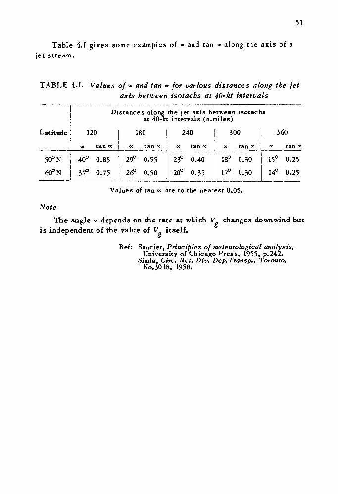
51
Table 4.1 gives some examples of « and tan « along the axis of a jet stream.
TABLE 4.1. Values of « and tan « (or various distances along the jetaxis between isotachs at 40-kt intervals\
Latitude
50°N
60° N_
Distances along the jet axis between isotachs at 40-kt intervals (rumiles)
120
<x
40°
37°
tan <x
0.85
0.75
180
« tan «
29° 0.55
2tf> 0.50
240« tan «
23° 0.40
20° 0.35.... . -i
300
« tan «
18° 0.30
17° 0.30
360
« tan «
15° 0.25
14° 0.25
Values of tan « are to the nearest 0.05.
Note
The angle « depends on the rate at which V changes downwind but is independent of the value of V itself.
o
Ref: Saucier, Principles of meteorological analysis,University of Chicago Press, 1955 t p.242.
Simla, Circ. Met. Div. Dep.Transp., Toronto, No. 3018, 1958.
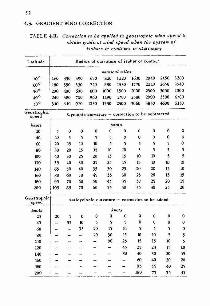
52
4.3. GRADIENT WIND CORRECTION
TABLE 4.II. Correction to be applied to geostrophic wind speed to obtain gradient wind speed when the system of
isobars or contours is stationary
Latitude
70°60°50°
Radius of curvature of isobar or contour
nautical miles160180200
40° 24030°
Geostrophic speed
knots20406080
100120140160180200
Geostrophic speed
knots20406080
100120140160180
310
330350400480610
490530600720920
Cyclonic
650710800960
1230
820880
100011901530
12201330150017902300
16301770200023803060
20402210250029803830
24502650300035804600
32603540400047606130
curvature — correction to be subtracted
knots5
1020304055658095
105
05
1520304050607085
05
1015253040506070
05
1015202535455060
055
10152530354555
Anticyclonic curvature
005
10151525303540
0055
101520253035
— correction
0055
101020202530
to be
00555
1015152025
added
00055
1010151520
knots20—-——————
200
535————————
01055———————
05
2070——————
05
153090—————
05
1015254580———
005
101525406095
180
005
10152030405575
0055
101520304055
00055
1015202535
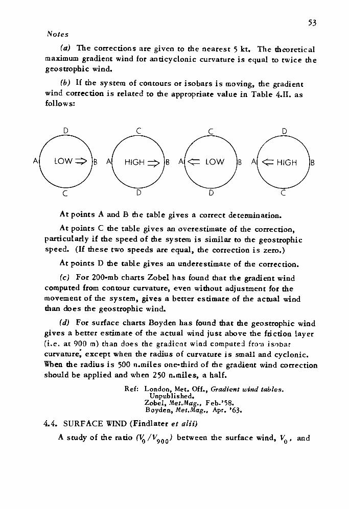
53 Notes
(a) The corrections are given to the nearest 5 kt. The theoretical maximum gradient wind for anticyclonic curvature is equal to twice the geostrophic wind.
(b) If the system of contours or isobars is moving, the gradient wind correction is related to the appropriate value in Table 4.II. as follows:
At points A and B the table gives a correct determination.At points C the table gives an overestimate of the correction,
particularly if the speed of the system is similar to the geostrophic speed. (If these two speeds are equal, the correction is zero.)
At points D the table gives an underestimate of the correction.(c) For 200-mb charts Zobel has found that the gradient wind
computed from contour curvature, even without adjustment for the movement of the system, gives a better estimate of die actual wind than does the geostrophic wind.
(d) For surface charts Boyden has found that the geostrophic wind gives a better estimate of the actual wind just above the friction layer (i.e. at 900 m) than does the gradieat wind computed fro-a isobar curvature^ except when the radius of curvature is small and cyclonic. When the radius is 500 n.miles one-third of the gradient wind correction should be applied and when 250 n.miles, a half.
Ref: London, Met. Off., Gradient wind tables.Unpublished.
Zobel, Met.Mag., Feb.'58. Boyden, Met.Mag., Apr. '63.
4.4. SURFACE WIND (Findlater et alii)A study of the ratio (VQ /^900 ^ between the surface wind, VQ , and
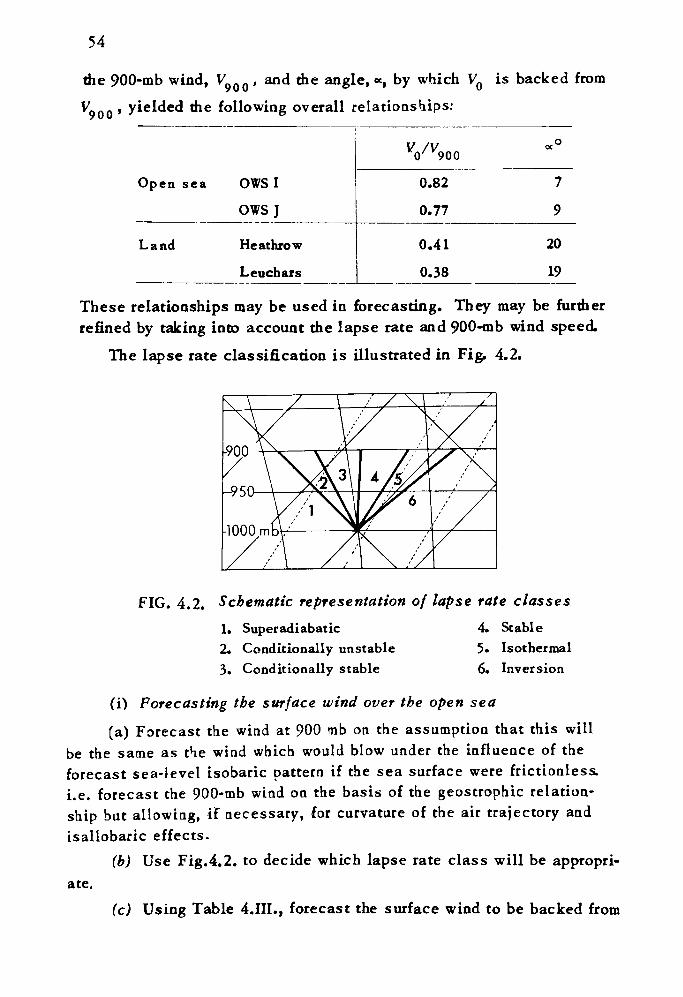
54
the 900-mb wind, V90Q , and the angle, «, by which VQ is backed from
900 the following overall relationships:
Open sea
Land
OWSI
OWS J
Heatkrow
Leuchars
V /V oe°0' 900
0.82
0.77
0.41
0.38
7
9
20
19
These relationships may be used in forecasting. They may be further refined by taking into account the lapse rate and 900-mb wind speed.
The lapse rate classification is illustrated in Fig. 4.2.
FIG. 4.2. Schematic representation of lapse rate classes
1. Superadiabatic 4. Stable
2. Conditionally unstable 5. Isothermal
3. Conditionally stable 6. Inversion
(i) Forecasting the surface wind over the open sea
(a) Forecast the wind at 900 mb on the assumption that this will
be the same as the wind which would blow under the influence of the forecast sea-level isobaric pattern if the sea surface were frictionless. i.e. forecast the 900-mb wind on the basis of the geostrophic relation ship but allowing, if necessary, for curvature of the air trajectory and isallobaric effects.
(b) Use Fig.4.2. to decide which lapse rate class will be appropriate.
(c) Using Table 4.IIL, forecast the surface wind to be backed from
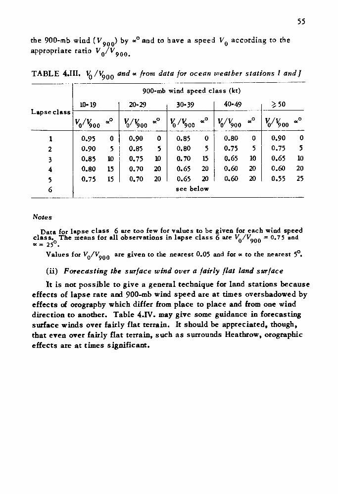
55
the 900-mb wind (V 900 ) by «° and to have a speed V Q according to the900 appropriate ratio V 0 /V 900>
TABLE 4.HI. and * from data for ocean vieather stations I and]
Lapse class
123456
10-19
VV900 «°
0.95 00.90 50.85 100.80 150.75 15
900-mb
20-29
W "°0.90 00.85 50.75 100.70 200.70 20
wind speed c
30-39w «°0.85 00.80 50.70 150.65 200.65 20
ass (kt)
40-49
VV900 «°
0.80 00.75 50.65 100.60 200.60 20
£50
VV900 -°
0.90 00.75 50.65 100.60 200.55 25
see below
Notes
Data for lapse class 6 are too few for values to be given for each wind speed class. The means for all observations in lapse class 6 are Vn/Vgnn = 0.75 and <* = 25°.
are given to the nearest 0.05 and for « to the nearest 5°.Values for V/y
(ii) Forecasting the surface wind over a fairly flat land surface
It is not possible to give a general technique for land stations because effects of lapse rate and 900-mb wind speed are at times overshadowed by effects of orography which differ from place to place and from one wind direction to another. Table 4.IV. may give some guidance in forecasting surface winds over fairly flat terrain. It should be appreciated, though, that even over fairly flat terrain, such as surrounds Heathrow, orographic effects are at times significant.
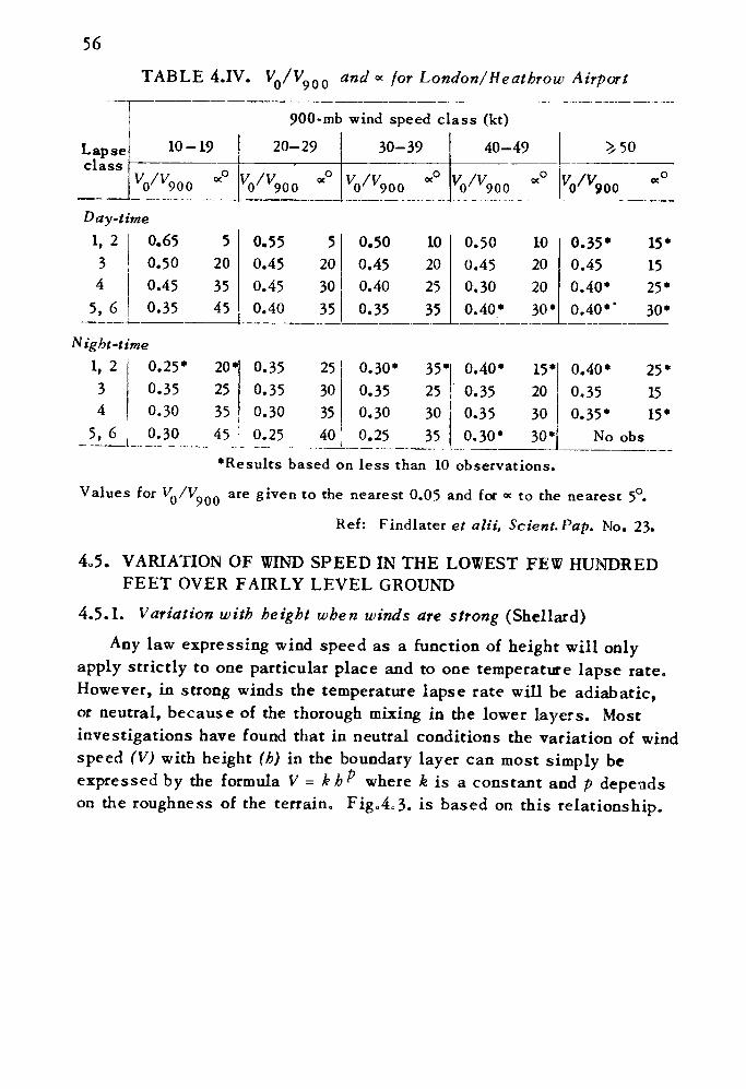
56TABLE 4.IV. V0/V9QO and « for London/'Heatbrow Airport
Lapse class
10-19
V^oo a°
900-mb
20-29
V /V <x° O x 900
wind speed cl
30-39
V /V *° O x 900
ass (kt)
40-49
V^900 «°
^50
V /V «° 0 900
Day-time1, 2345,6
0.65 50.50 200.45 350.35 45
0.55 50.45 200.45 300.40 35
0.50 100.45 200.40 250.35 35
0.50 100.45 200.30 200.40* 30*
0.35* 15*0.45 150.40* 25*0.40*' 30*
Night-time1, 234
0.25* 20*0.35 250.30 35
5, 6 . 0.30 45
0.35 25 j 0.30* 35*0.35 300.30 350.25 40
0.35 250.30 300.25 35
0.40* 15*0.35 200.35 300.30* 30*
0.40* 25*0.35 150.35* 15*
No obs
Values for VQ /V,900
'Results based on less than 10 observations,
are given to the nearest 0.05 and for « to the nearest 5°.
Ref: Findlater et alii, Scient.Pap. No. 23.
4,5. VARIATION OF WIND SPEED IN THE LOWEST FEW HUNDRED FEET OVER FAIRLY LEVEL GROUND
4.5.1. Variation with height when winds are strong (Shellard)Any law expressing wind speed as a function of height will only
apply strictly to one particular place and to one temperature lapse rate. However, in strong winds the temperature lapse rate will be adiabatic, or neutral, because of the thorough mixing in the lower layers. Most investigations have found that in neutral conditions the variation of wind speed (V) with height (h) in the boundary layer can most simply be expressed by the formula V = kh " where k is a constant and p depends on the roughness of the terrain, Fig»4<,3. is based on this relationship.
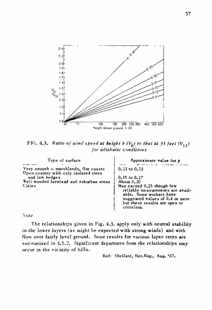
57
50 100 150 200 250 300 Height above ground, h
400 500 600
FIG. 4.3. Ratio of wind speed at height b (V^) to that at 33 feetfor adiabatic conditions
Type of surface
Very smooth — marshlands, flat coasts Open country with only isolated trees
and low hedgesWell wooded farmland and suburban areas Cities
Approximate value for p
0.11 to 0.13
0.15 to 0.17About 0.20May exceed 0.25 though few
reliable measurements are avail able. Some workers have suggested values of 0.4 or more but these results are open to criticism.
Xote
The relationships given in Fig. 4.3. apply only with neutral stability in the lower layers (as might be expected with strong winds) and with flow over fairly level ground. Some results for various lapse rates are summarized in 4.5.2. Significant departures from the relationships may occur in the vicinity of hills.
Ref: Shellard, Met.Mag., Aug. '67.
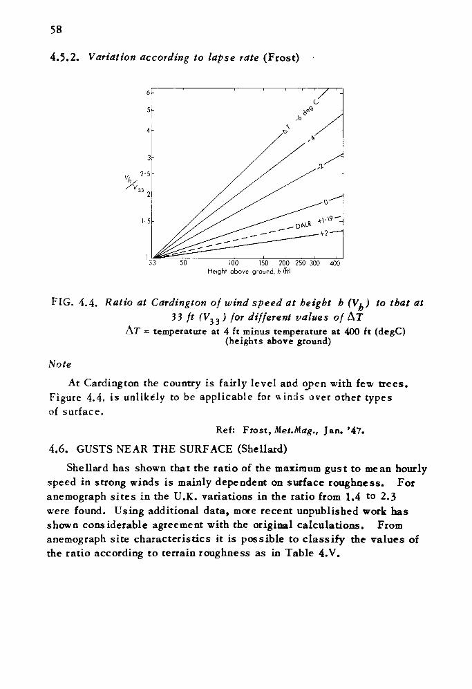
58
4.5.2. Variation according to lapse rate (Frost)
50 100 150 200 250 300 Height above ground. /> (ft)
400
FIG. 4.4. Ratio at Cardington of wind speed at height h (V^) to that at33 ft (V33 ) for different values of AT
AT = temperature at 4 ft minus temperature at 400 ft (degC)(heights above ground)
NoteAt Cardington the country is fairly level and open with few trees.
Figure 4.4. is unlikely to be applicable for winds over other types of surface.
Ref: Frost, Met.Mag., Jan. '47.
4.6. GUSTS NEAR THE SURFACE (Shellard)
She liar d has shown that the ratio of the maximum gust to mean hourly speed in strong winds is mainly dependent on surface roughness. For anemograph sites in the U.K. variations in the ratio from 1.4 to 2.3 were found. Using additional data, more recent unpublished work has shown considerable agreement with the original calculations. From anemograph site characteristics it is possible to classify the values of the ratio according to terrain roughness as in Table 4.V.
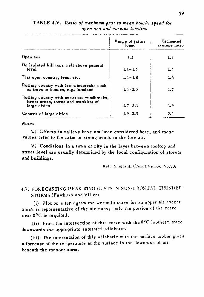
59TABLE 4.V. Ratio of maximum gust to mean hourly speed for
open sea and various terrains
Open sea
On isolated hill tops well above general level
Flat open country, fens, etc.
Rolling country with few windbreaks such as trees or houses, e.g. farmland
Rolling country with numerous windbreaks, forest areas, towns and outskirts of large cities
Centres of large cities
Notes
Range of ratios found
Estimated average ratio
1.3
1.4-1.5
1.4-1.8
1.5-2.0
1.7-2.1
1.9-2.3
1.3
1.4
1.6
1.7
1.9
(a) Effects in valleys have not been considered here, and these values refer to the ratio in strong winds in the free air.
(b) Conditions in a town or city in the layer between rooftop and street level are usually determined by the local configuration of streets and buildings.
Ref: Shellard, Climat.Memor. No.50.
4.7. FORECASTING PEAK WIND GUSTS IN NON-FRONTAL THUNDER STORMS (Fawbush and Miller) (i) Plot on a tephigram the wet-bulb curve for an upper air ascent
which is representative of the air mass; only the portion of the curvenear 0°C is required.
(ti) From the intersection of this curve with the 0°C isotherm tracedownwards the appropriate saturated adiabatic.
(Hi) The intersection of this adiabatic with the surface isobar givesa forecast of the temperature at the surface in the downrush of airbeneath the thunderstorm.
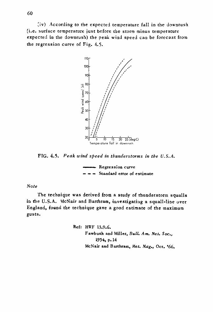
60
jv) According to the expected temperature fall in the downrush (i.e. surface temperature just before the storm minus temperature expected in the downrush) the peak wind speed can be forecast from the regression curve of Fig. 4.5.
U0 5 10 15 20 25(degC) Temperature fall in downrush
FIG. 4.5. Peak wind speed in thunderstorms in the U.S.A.
'in • • Regression curve — — — Standard error of estimate
Note
The technique was derived from a study of thunderstorm squalls in the U.S.A. McNair and Barthram, investigating a squall-line over England, found the technique gave a good estimate of the maximum gusts.
Ref: HWF 13.9.6.Fawbush and Miller, Bull. Am. Met. Soc.,
1954, p. 14 McNair and Barthram, Met. Mag., Oct. '66.
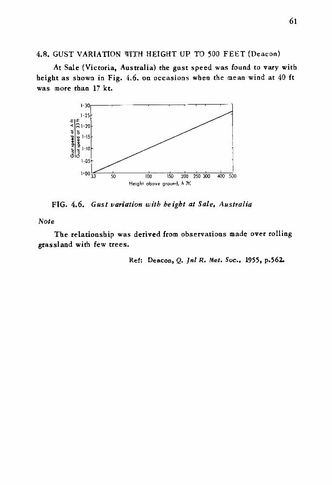
61
4.8. GUST VARIATION WITH HEIGHT UP TO 500 FEET (Deacon)
At Sale (Victoria, Australia) the gust speed was found to vary with height as shown in Fig. 4.6. on occasions when the mean wind at 40 ft was more than 17 kt.
1-0050 100 ISO 200 250 300 400 500
Height above ground, h (ft)
FIG. 4.6. Gust variation with height at Sale, Australia
Note
The relationship was derived from observations made over rolling grassland with few trees.
Ref: Deacon, Q. Jnl R. Met. Soc.. 1955, p.562.
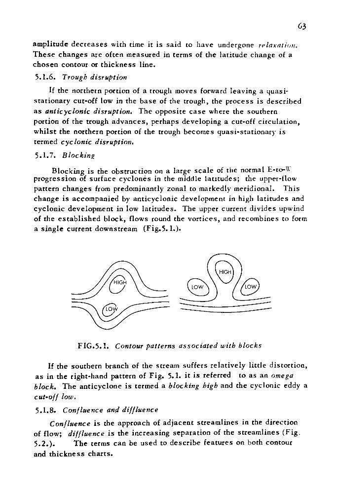
63
amplitude decreases with time it is said to have undergone relaxation. These changes are often measured in terms of the latitude change of a chosen contour or thickness line.5.1.6. Trough disruption
If the northern portion of a trough moves forward leaving a quasi- stationary cut-off low in the base of the trough, the process is described as anticyclonic disruption. The opposite case where the southern portion of the trough advances, perhaps developing a cut-off circulation, whilst the northern portion of the trough becomes quasi-stationary is termed cyclonic disruption.
5.1.7. Blocking
Blocking is the obstruction on a large scale of the normal E-to-\X progression of surface cyclones in the middle latitudes; the upper-flow pattern changes from predominantly zonal to markedly meridional. This change is accompanied by anticyclonic development in high latitudes and cyclonic development in low latitudes. The upper current divides upwind of the established block, flows round the vortices, and recombines to form a single current downstream (Fig.5.1.).
FIG.5.1. Contour patterns associated with blocks
If the southern branch of the stream suffers relatively little distortion, as in the right-hand pattern of Fig. 5.1. it is referred to as an omega block. The anticyclone is termed a blocking high and the cyclonic eddy a cut-off low. 5.1.8. Confluence and diffluence
Confluence is the approach of adjacent streamlines in the direction of flow; diffluence is the increasing separation of the streamlines (Fig. 5.2.). The terms can be used to describe features on both cdntour and thickness charts.
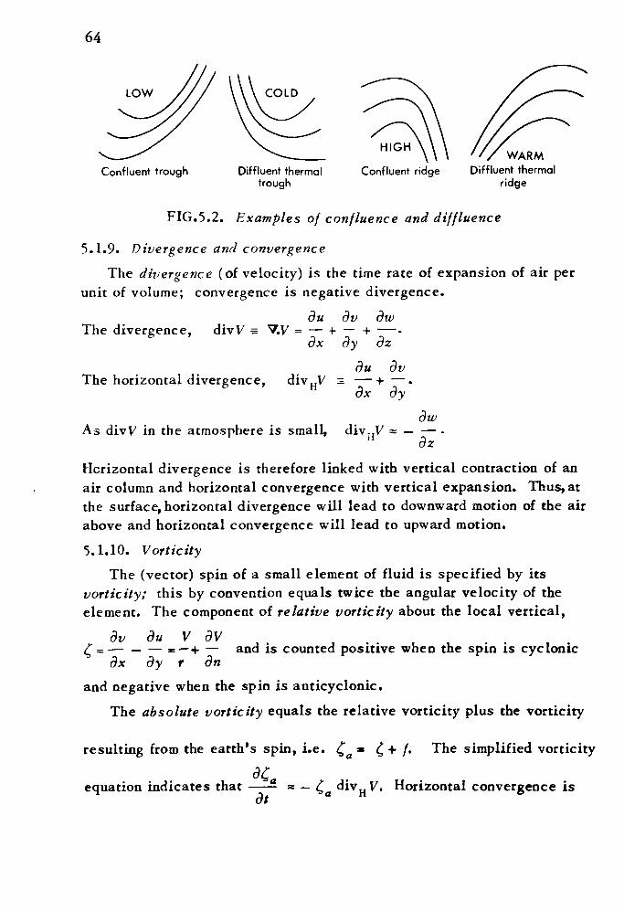
64
Confluent trough Diffluent thermal trough
HIGH
Confluent ridgeWARM
Diffluent thermal ridge
FIG. 5. 2. Examples of confluence and diffluence
5.1.9. Divergence and convergence
The divergence (of velocity) is the time rate of expansion of air per unit of volume; convergence is negative divergence.
The divergence, divV =
The horizontal divergence,
du dv dw= — + — + — -
dx dy dz
du dvdiv HV = — + — •
dx dy
dw As divV in the atmosphere is small, div..V = — — -
dz
Horizontal divergence is therefore linked with vertical contraction of an air column and horizontal convergence with vertical expansion. Thus, at the surface, horizontal divergence will lead to downward motion of the air above and horizontal convergence will lead to upward motion.
5.1.10. Vorticity
The (vector) spin of a small element of fluid is specified by its vorticity; this by convention equals twice the angular velocity of the element. The component of relative vorticity about the local vertical,
dv du V dV £ = — — — * — + — and is counted positive when the spin is cyclonic
dx dy r dn
and negative when the spin is anticyclonic.
The absolute vorticity equals the relative vorticity plus the vorticity
resulting from the earth's spin, i.e. £ + /. The simplified vorticity
equation indicates that ——- « — £a div H V. Horizontal convergence isdt
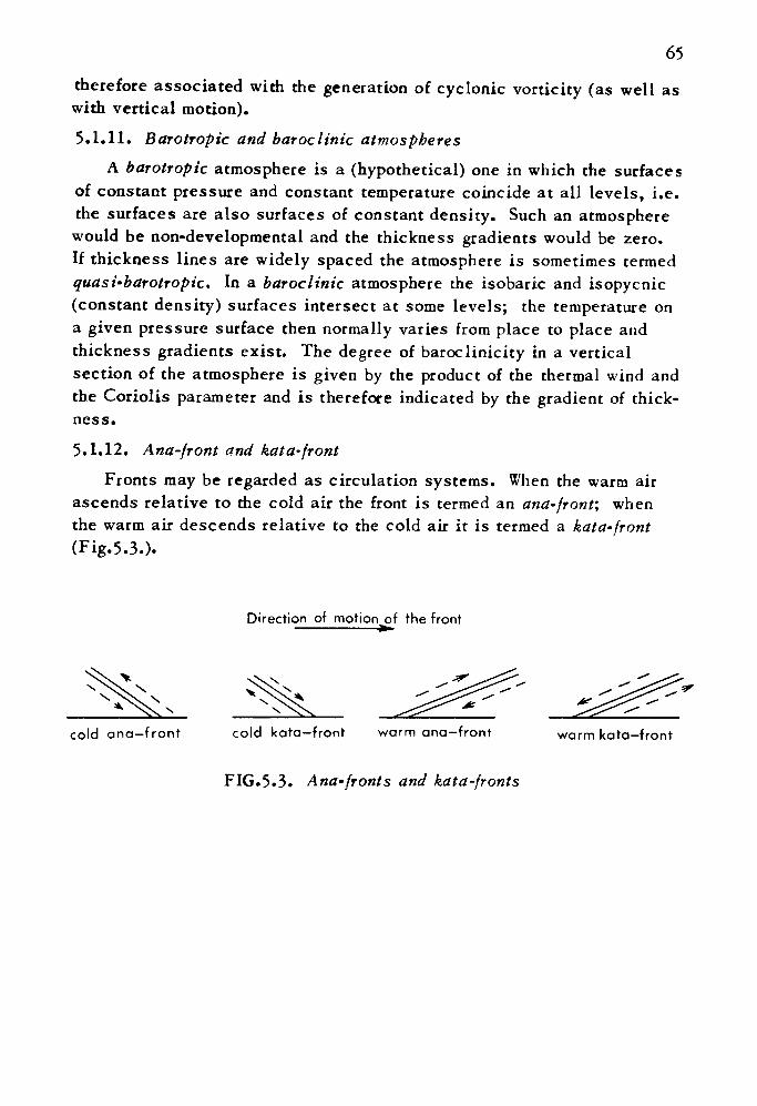
65therefore associated with the generation of cyclonic vorticity (as well as with vertical motion).
5.1.11. Barotropic and baroclinic atmospheresA barotropic atmosphere is a (hypothetical) one in which the surfaces
of constant pressure and constant temperature coincide at all levels, i.e. the surfaces are also surfaces of constant density. Such an atmosphere would be non-developmental and the thickness gradients would be zero. If thickness lines are widely spaced the atmosphere is sometimes termed quasi-barotropic. In a baroclinic atmosphere the isobaric and isopycnic (constant density) surfaces intersect at some levels; the temperature on a given pressure surface then normally varies from place to place and thickness gradients exist. The degree of baroclinicity in a vertical section of the atmosphere is given by the product of the thermal wind and the Coriolis parameter and is therefore indicated by the gradient of thick ness.
5.1.12. Ana-front and kata-frontFronts may be regarded as circulation systems. When the warm air
ascends relative to the cold air the front is termed an ana-front', when the warm air descends relative to the cold air it is termed a kata-front (Fig.5.3.).
Direction of motion of the front
cold ana—front cold kata-front warm ana-front warm kata—front
FIG.5.3. Ana-fronts and kata-fronts
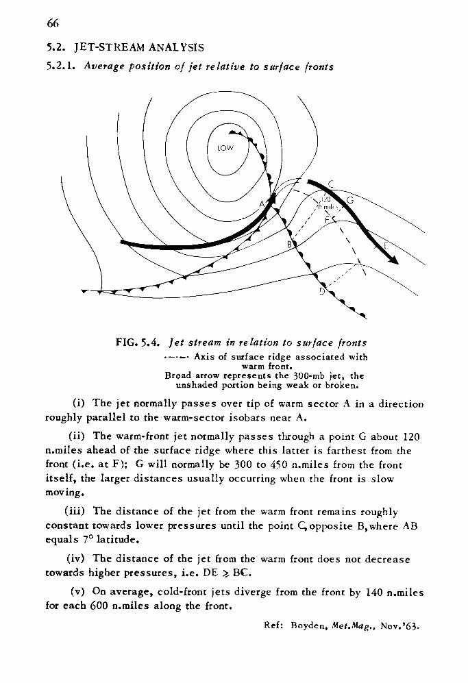
66
5.2. JET-STREAM ANALYSIS5.2.1. Average position of jet relative to surface fronts
FIG. 5.4. Jet stream in relation to surface fronts• ——' Axis of surface ridge associated with
warm front.Broad arrow represents the 300-mb jet, the
unshaded portion being weak or broken.
(i) The jet normally passes over tip of warm sector A in a direction roughly parallel to the warm-sector isobars near A.
(ii) The warm-front jet normally passes tlirough a point G about 120 n.miles ahead of the surface ridge where this latter is farthest from the front (i.e. at F); G will normally be 300 to 450 n.miles from the front itself, the larger distances usually occurring when the front is slow moving.
(iii) The distance of the jet from the warm front remains roughly constant towards lower pressures until the point C, opposite B,where AB equals 7° latitude.
(iv) The distance of the jet from the warm front does not decrease towards higher pressures, i.e. DE ^ BC.
(v) On average, cold-front jets diverge from the front by 140 n.miles for each 600 n.miles along the front.
Ref: Boyden, Met. Mag.. Nov.'63-
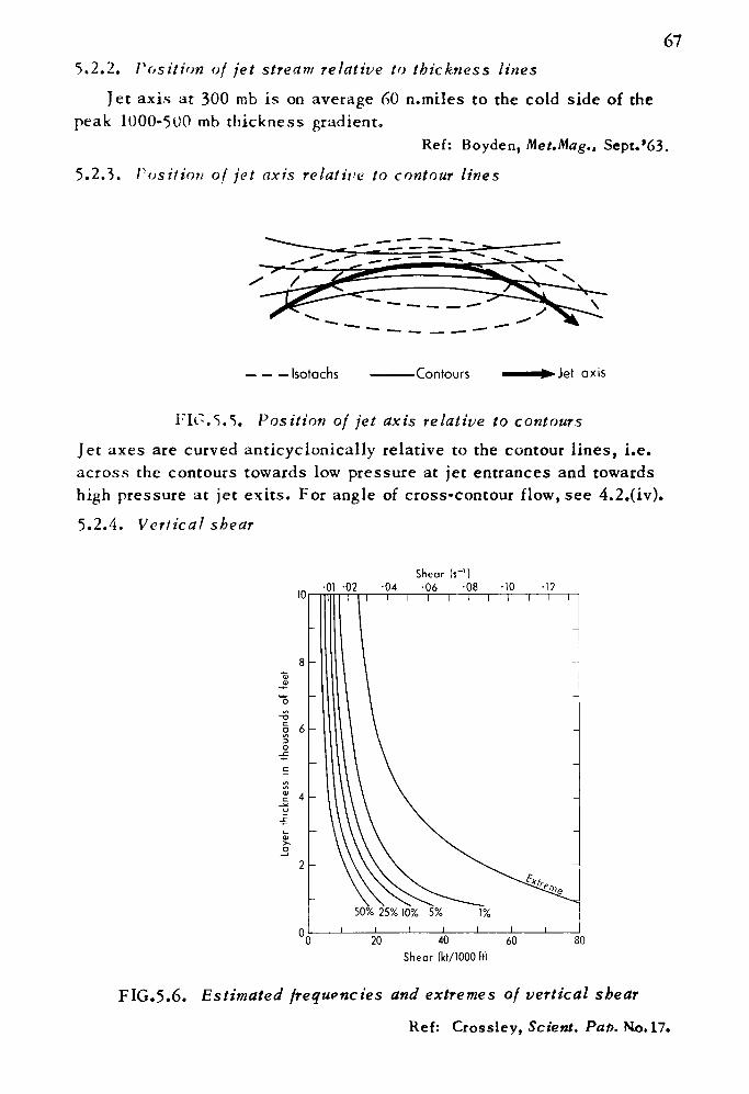
675.2.2. Position of jet stream relative to thickness lines
Jet axis at 300 mb is on average 60 n.miles to the cold side of the peak 1000-500 mb thickness gradient.
Ref: Boyden, Met.Mag., Sept.'63.
5.2.3. Position of jet axis relative to contour lines
— — — Isotachs -Contours • Jet axis
FIG.5.5. Position of jet axis relative to contours
Jet axes are curved anticyclonically relative to the contour lines, i.e. across the contours towards low pressure at jet entrances and towards high pressure at jet exits. For angle of cross-contour flow, see 4.2.(iv).
5.2.4. Vertical shear
10•01 -02 •04
Shear Is' 1 ) •06 -08 •10 •12
§ 6
1 I I I T
50% 25% 10% 5%i___i___i_
1%
20 40 60 Shear (let/1000 ft)
80
FIG.5.6. Estimated frequencies and extremes of vertical shear
Ref: Crossley, Scient. Pat), Mo. 17.
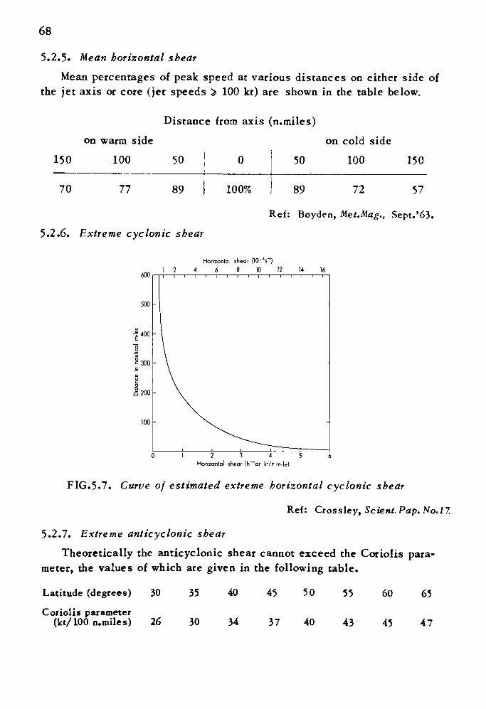
68
5.2.5. Mean horizontal shear
Mean percentages of peak speed at various distances on either side of the jet axis or core (jet speeds > 100 kt) are shown in the table below.
Distance from axis (n.miles)
on warm side on cold side
150
70
100
77
50
89
0
100%
50
89
100
72
150
57
Ref: Boyden, Met.Mag., Sept.'63.
5.2.6. Extreme cyclonic shear
Horizontal shear (1CTV) 1 2 4 6 8 10 12 14 16
12345 Horizontal shear (h~'or kt/n.mile)
FIG.5.7. Curve of estimated extreme horizontal cyclonic shear
Ref: Crossley, Scient. Pap. No.17.
5.2.7. Extreme anticycIonic shear
Theoretically the anticyclonic shear cannot exceed the Coriolis para meter, the values of which are given in the following table.
Latitude (degrees) 30 35 40 45 50 55 60 65
Coriolis parameter(kt/100 n.miles) 26 30 34 37 40 43 45 47
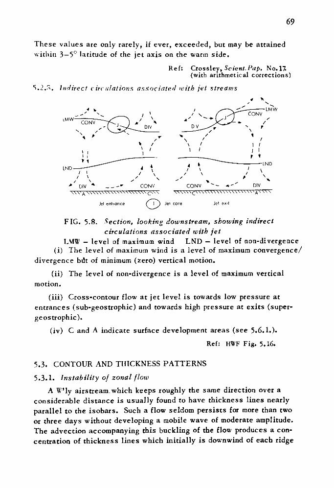
69
These values are only rarely, if ever, exceeded, but may be attained within 3-5° latitude of the jet axis on the warm side.
Ref: Crossley, Scient. Pap. No.17. (with arithmetical corrections)
5.2.S. Indirect circulations associated with jet streams
LMW
LND
CONV CONV\\N\\\\\\\\N\\N
Jet entrance
r^x \\\\\\£\\\\\\\\\\\\\\\\\\\^
Jet core Jet exit
FIG. 5.8. Section, looking downstream, showing indirectcirculations associated with jet
LVfW — level of maximum wind LND — level of non-divergence (i) The level of maximum wind is a level of maximum convergence/
divergence bdt of minimum (zero) vertical motion.
(ii) The level of non-divergence is a level of maximum vertical motion.
(iii) Cross-contour flow at jet level is towards low pressure at entrances (sub-geostrophic) and towards high pressure at exits (super- ge os trophic).
(iv) C and A indicate surface development areas (see 5.6.1.).
Ref: HWF Fig. 5.16.
5.3. CONTOUR AND THICKNESS PATTERNS
5.3.1. Instability of zonal flow
A W'ly airstream. which keeps roughly the same direction over a considerable distance is usually found to have thickness lines nearly parallel to the isobars. Such a flow seldom persists for more than two or three days without developing a mobile wave of moderate amplitude. The advection accompanying this buckling of the flow produces a con centration of thickness lines which initially is downwind of each ridge
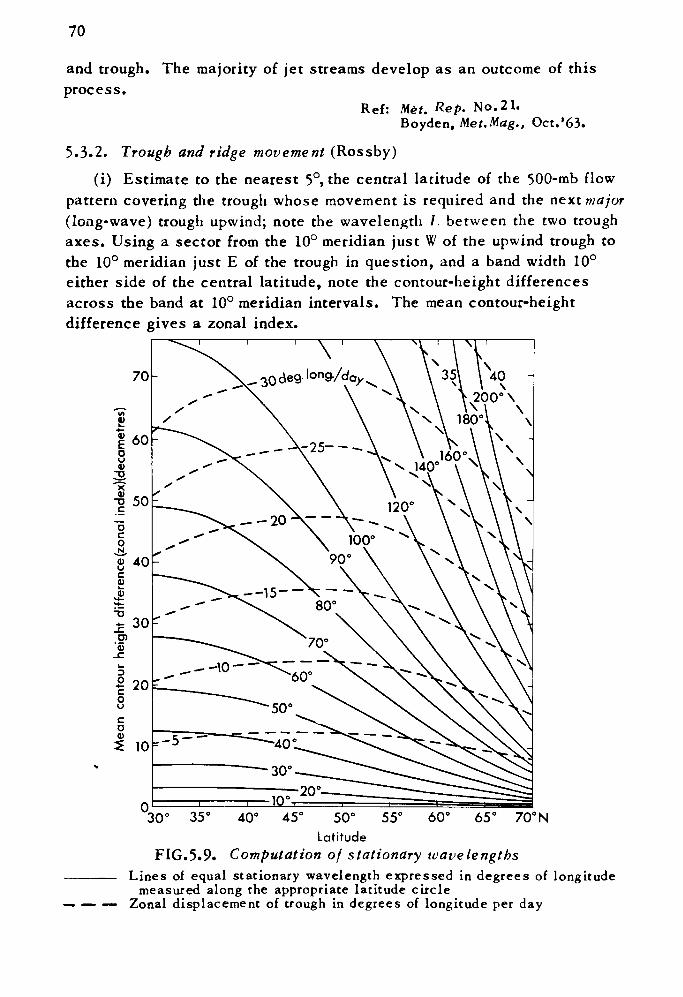
70
and trough. The majority of jet streams develop as an outcome of this process.
Ref: Met. Rep. No. 21.Boyden, Met.Mag., Oct.'63.
5.3.2. Trough and ridge movement (Rossby)
(i) Estimate to the nearest 5°, the central latitude of the 500-mb flow pattern covering the trough whose movement is required and the next major (long-wave) trough upwind; note the wavelength / between the two trough axes. Using a sector from the 10° meridian just W of the upwind trough to the 10° meridian just E of the trough in question, and a band width 10° either side of the central latitude, note the contour-height differences across the band at 10° meridian intervals. The mean contour-height difference gives a zonal index.
30° 40° 45 55° 60° 65° 70°N50° Latitude
FIG.5.9. Computation of stationary wavelengthsLines of equal stationary wavelength expressed in degrees of longitude
measured along the appropriate latitude circle Zonal displacement of trough in degrees of longitude per day
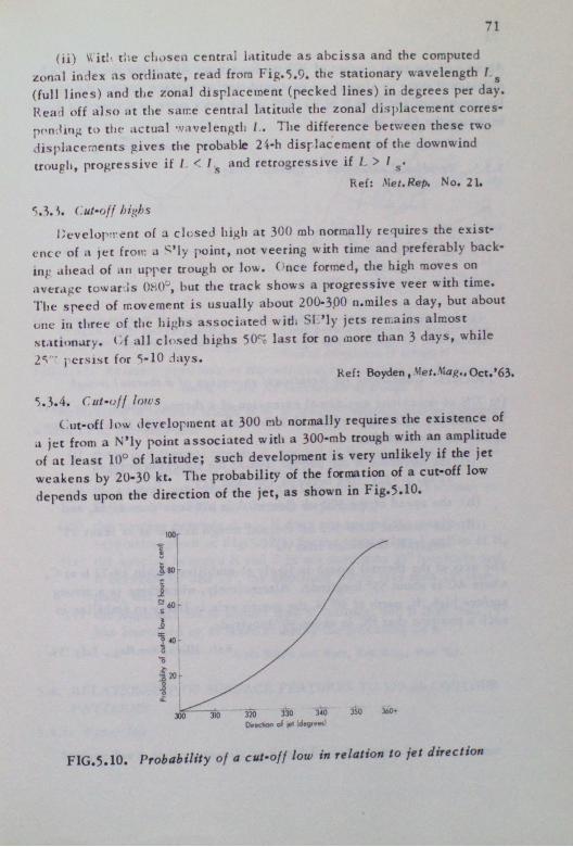
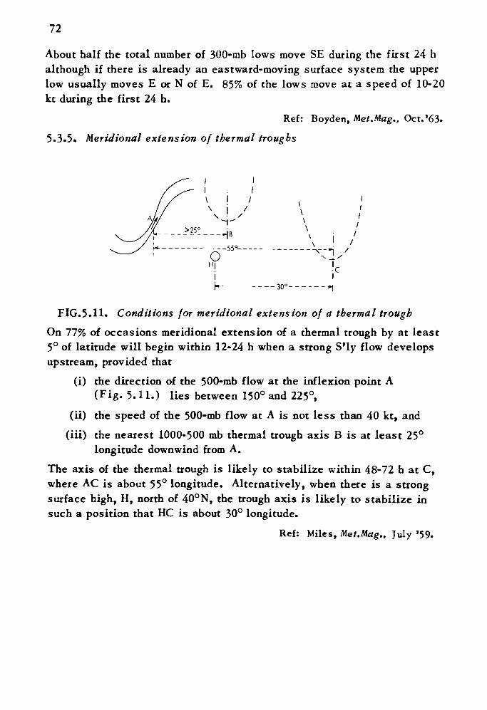
72
About half the total number of 300-mb lows move SE during the first 24 h although if there is already an eastward-moving surface system the upper low usually moves E or N of E. 85% of the lows move at a speed of 10-20 kt during the first 24 h.
Ref: Boyden, Met.Mag., Oct.'63.
5.3.5. Meridional extension of thermal troughs
FIG.5.H. Conditions for meridional extension of a thermal trough
On 77% of occasions meridional extension of a thermal trough by at least 5° of latitude will begin within 12-24 h when a strong S'ly flow develops upstream, provided that
(i) the direction of the 500-mb flow at the inflexion point A (Fig. 5.11.) lies between 150° and 225°,
(ii) the speed of the 500-mb flow at A is not less than 40 kt, and
(iii) the nearest 1000-500 mb thermal trough axis B is at least 25° longitude downwind from A.
The axis of the thermal trough is likely to stabilize within 48-72 h at C, where AC is about 55° longitude. Alternatively, when there is a strong surface high, H, north of 40°N, the trough axis is likely to stabilize in such a position that HC is about 30° longitude.
Ref: Miles, Met.Mag., July '59.
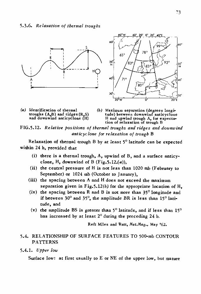
5.3.6. Relaxation of thermal troughs
60" W 40° 20° 0' 20° 40°E
30°'30°
20° W 20°E
(a) Identification of thermaltroughs (A,B) and ridges (R.S) and downwind anticyclone (H)
(b) Maximum separation (degrees longi tude) between downwind anticyclone H and upwind trough A, for expecta tion of relaxation of trough B
FIG.5.12. Relative positions of thermal troughs and ridges and downwindanticyclone for relaxation of trough B
Relaxation of thermal trough B by at least 5° latitude can be expected within 24 h, provided that
(i) there is a thermal trough, A, upwind of B, and a surface anticy clone, H, downwind of B (Fig.5.12.(a)),
(ii) the central pressure of H is not less than 1020 mb (February toSeptember) or 1024 mb (October to January),
(iii) the spacing between A and H does not exceed the maximumseparation given in Fig.5.12(&) for the appropriate location of H,
(iv) the spacing between R and B is not more than 35° longitude and if between 30° and 35°, the amplitude BR is less than 15° lati tude, and
(v) the amplitude BS is greater than 5° latitude, and if less than 15° has increased by at least 2° during the preceding 24 h.
Ref: Miles and Watt, Met.Mag., May '62.
5.4. RELATIONSHIP OF SURFACE FEATURES TO 500-mb CONTOUR PATTERNS
5.4.1. Upper lowSurface low: at first usually to E or NE of the upper low, but mature
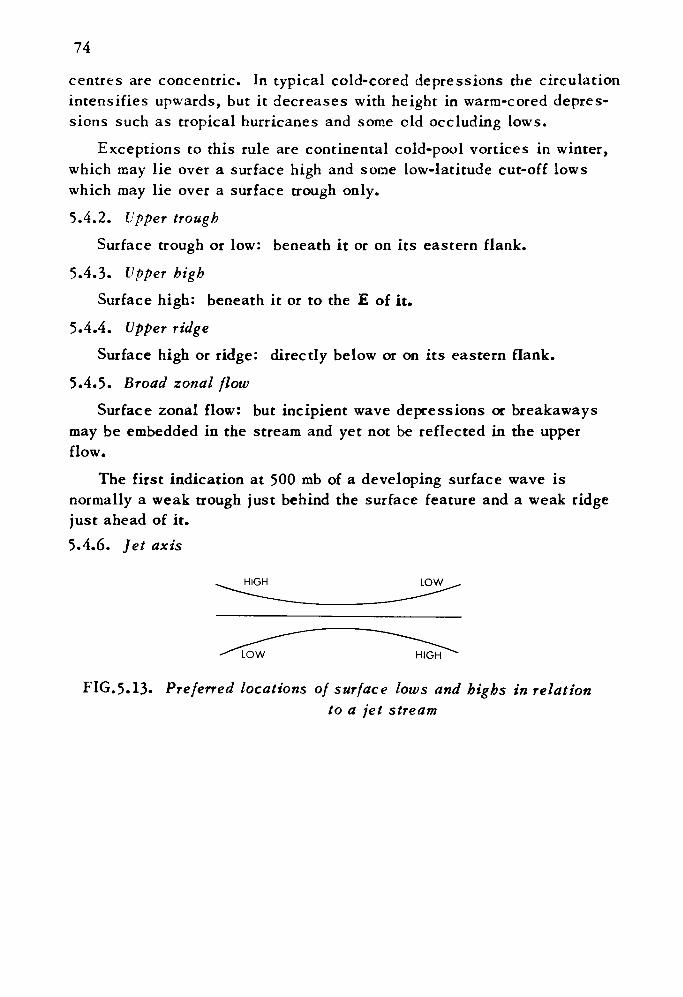
74
centres are concentric. In typical cold-cored depressions the circulation intensifies upwards, but it decreases with height in warm-cored depres sions such as tropical hurricanes and some old occluding lows.
Exceptions to this rule are continental cold-pool vortices in winter, which may lie over a surface high and some low-latitude cut-off lows which may lie over a surface trough only.
5.4.2. Upper trough
Surface trough or low: beneath it or on its eastern flank.
5.4.3. Upper high
Surface high: beneath it or to the £ of it.
5.4.4. Upper ridge
Surface high or ridge: directly below or on its eastern flank.
5.4.5. Broad zonal flow
Surface zonal flow: but incipient wave depressions or breakaways may be embedded in the stream and yet not be reflected in the upper flow.
The first indication at 500 mb of a developing surface wave is normally a weak trough just behind the surface feature and a weak ridge just ahead of it.5.4.6. Jet axis
HIGH LOW
LOW
FIG.5.13. Preferred locations of surface lows and highs in relationto a jet stream
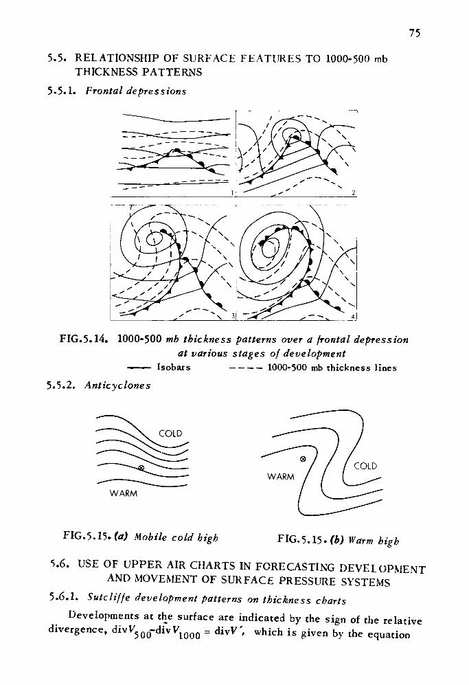
75
5.5. RELATIONSHIP OF SURFACE FEATURES TO 1000-500 mb THICKNESS PATTERNS
5.5.1. Frontal depressions
FIG.5.14. 1000-500 mb thickness patterns over a frontal depressionat various stages of development
——— Isobars ____ 1000-500 mb thickness lines
5.5.2. Anticyclones
WARM
FIG.5.15. (a) Mobile cold high FIG.5.15. (b) Warm high
5.6. USE OF UPPER AIR CHARTS IN FORECASTING DEVELOPMENT AND MOVEMENT OF SURFACE PRESSURE SYSTEMS
5.6.1. Sutcliffe development patterns on thickness chartsDevelopments at the surface are indicated by the sign of the relative
divergence, divV50o~c^v ^lOOO = divV, which is given by the equation
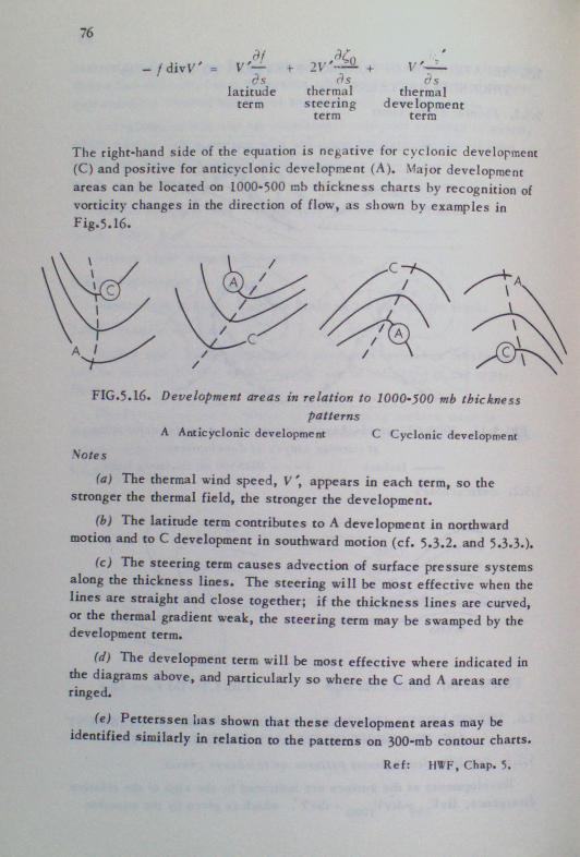
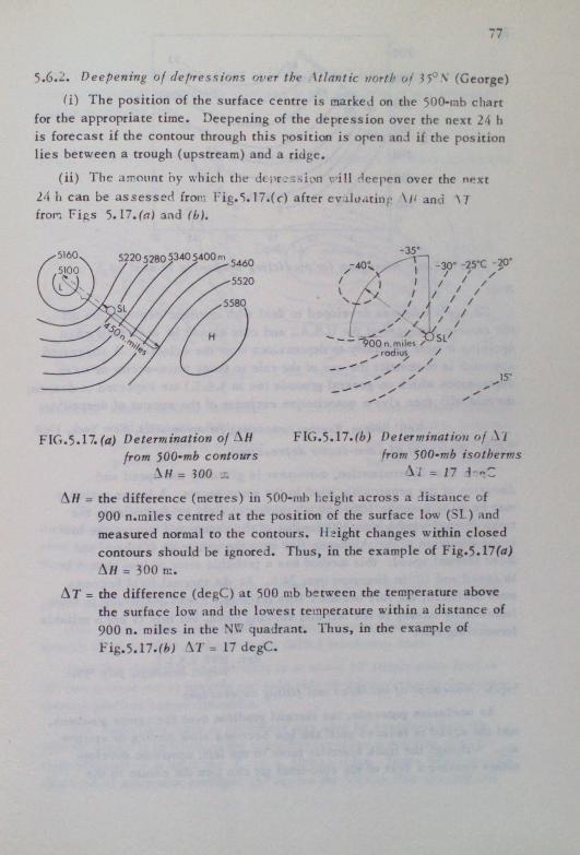
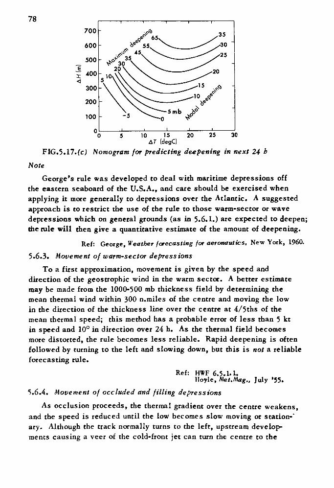
78700
600
500
400
300
200
100
0
-5
10 15(degC)
20 25 30
FIG.5.17. (c) Nomogram for predicting deepening in next 24 b
Note
George's rule was developed to deal with maritime depressions off the eastern seaboard of the U.S.A., and care should be exercised when applying it more generally to depressions over the Atlantic. A suggested approach is to restrict the use of the rule to those warm-sector or wave depressions which on general grounds (as in 5.6.1.) are expected to deepen; the rule will then give a quantitative estimate of the amount of deepening.
Ref: George, Weather forecasting for aeronautics. New York, I960.
5.6.3. Movement of warm~sector depressions
To a first approximation, movement is given by the speed and direction of the geostrophic wind in the warm sector. A better estimate may be made from the 1000-500 mb thickness field by determining the mean thermal wind within 300 n.miles of the centre and moving the low in the direction of the thickness line over the centre at 4/5ths of the mean thermal speed; this method has a probable error of less than 5 kt in speed and 10° in direction over 24 h. As the thermal field becomes more distorted, the rule becomes less reliable. Rapid deepening is often followed by turning to the left and slowing down, but this is not a reliable forecasting rule.
Ref: HWF 6.5.1.1.Hoyle, Ale/.Alag.. July '55.
5.6.4. Movement of occluded and filling depressions
As occlusion proceeds, the thermal gradient over the centre weakens, and the speed is reduced until the low becomes slow moving or station-" ary. Although the track normally turns to the left, upstream develop ments causing a veer of the cold-front jet can turn the centre to the
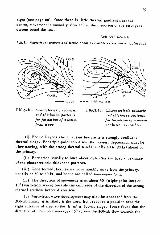
79
right (see page 80). Once there is little thermal gradient near the centre, movement is normally slow and in the direction of the strongest current round the low.
Ref: hWF 6.5.1.1. 5.6.5. Warm-front waves and triple-point secondaries on warm occlusions
COLD
FIG.5.18. Characteristic isobaric and thickness patterns for formation of a warm- front wave
Isobars — — — Thickness lines
FIG.5.19^ Characteristic isobaric and thickness patterns for formation of a warm- occlusion secondary
(i) For both types the important feature is a strongly confluent thermal ridge. For triple-point formation, the primary depression must be slow moving, with the strong thermal wind (usually 40 to 80 kt) ahead of the primary.
(ii) Formation usually follows about 24 h after the first appearance of the characteristic thickness patterns.
(iii) Once formed, both types move quickly away from the primary, usually at 30 to 50 kt, and hence are called breakaway lows.
(iv) The direction of movement is at about 30° (triple-point low) or 10° (warm-front wave) towards the cold side of the direction of the strong thermal gradient before distortion.
(v) Warm-front wave development may also be assessed from the 300-mb chart; it is likely if the warm front reaches a position near the right entrance of a jet to the E of a 300-mb ridge. Jones found that the direction of movement averages 15° across the 300-mb flow towards the
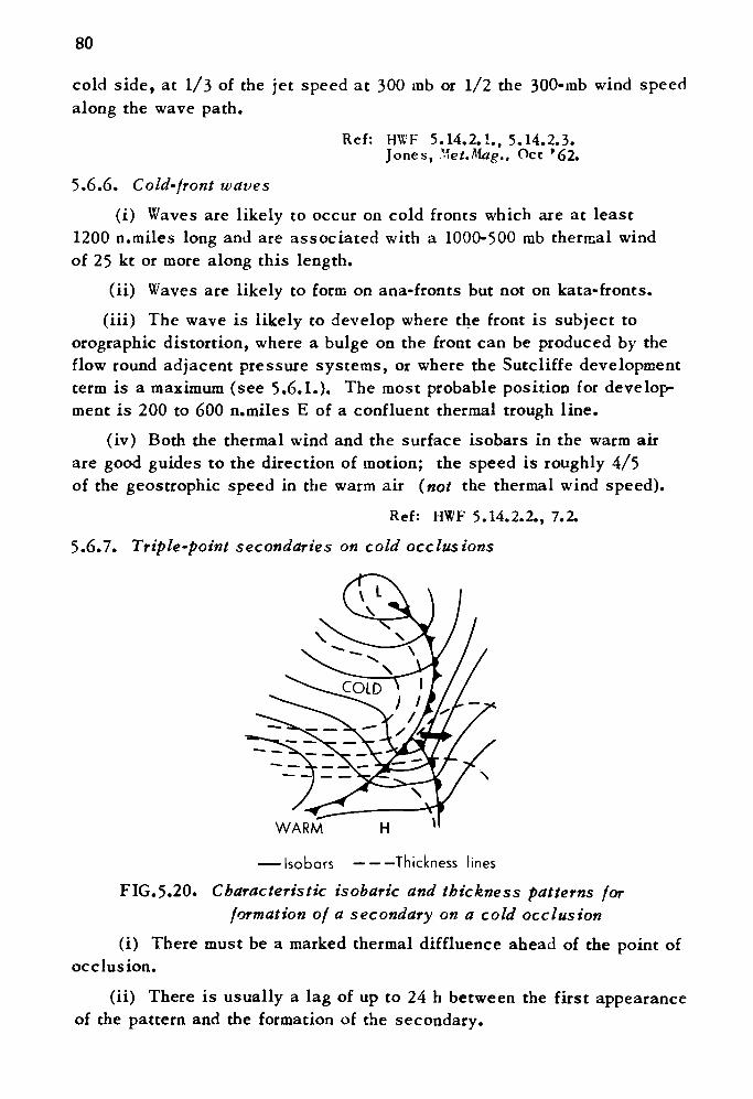
80
cold side, at 1/3 of the jet speed at 300 mb or 1/2 the 300-mb wind speed along the wave path.
Ref: H\VF 5.14.2.1., 5.14.2.3. Jones, Vet.Mag., Oct '62.
5.6.6. Cold-front waves
(i) Waves are likely to occur on cold fronts which are at least 1200 n.miles long and are associated with a 1000-500 mb thermal wind of 25 kt or more along this length.
(ii) Waves are likely to form on ana-fronts but not on kata-fronts.
(iii) The wave is likely to develop where the front is subject to orographic distortion, where a bulge on the front can be produced by the flow round adjacent pressure systems, or where the Sutcliffe development term is a maximum (see 5.6.1.). The most probable position for develop ment is 200 to 600 n.miles E of a confluent thermal trough line.
(iv) Both the thermal wind and the surface isobars in the warm air are good guides to the direction of motion; the speed is roughly 4/5 of the geostrophic speed in the warm air (not the thermal wind speed).
Ref: HWF 5.14.2.2., 7.2.
5.6.7. Triple-point secondaries on cold occlusions
WARM H
—— Isobars — — —Thickness lines
FIG.5.20. Characteristic isobaric and thickness patterns for formation of a secondary on a cold occlusion
(i) There must be a marked thermal diffluence ahead of the point of occlusion.
(ii) There is usually a lag of up to 24 h between the first appearance of the pattern and the formation of the secondary.
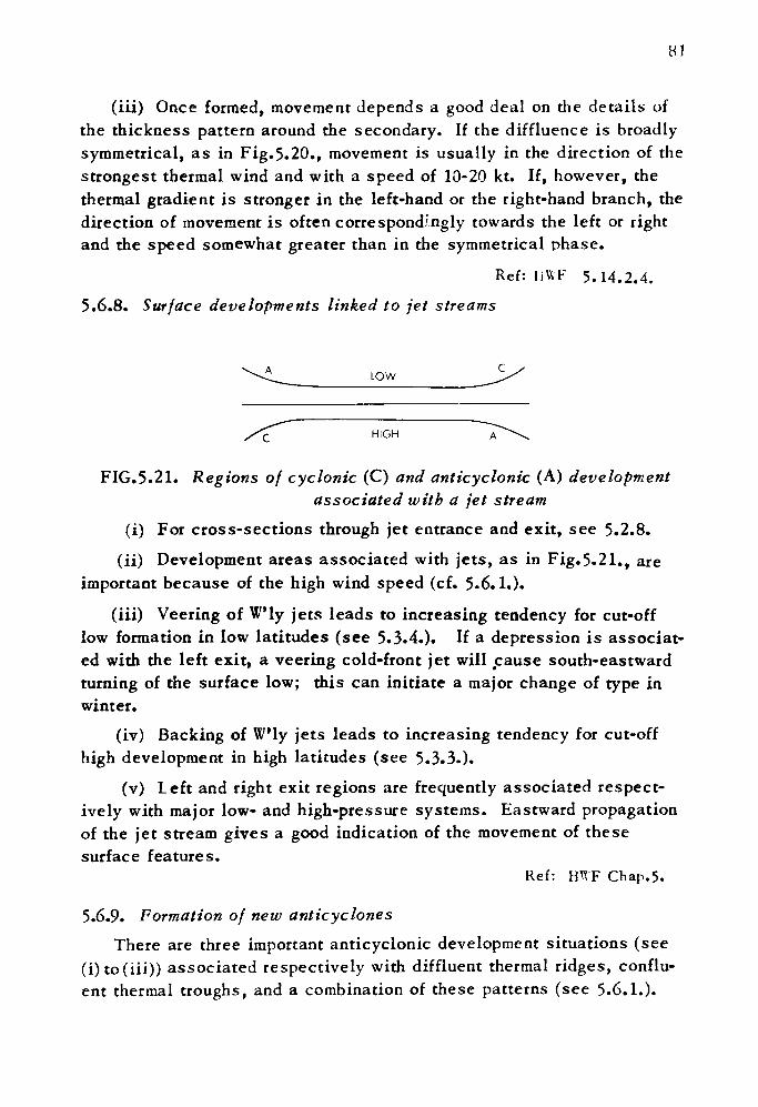
HI
(iii) Once formed, movement depends a good deal on the details of the thickness pattern around the secondary. If the diffluence is broadly symmetrical, as in Fig.5.20., movement is usually in the direction of the strongest thermal wind and with a speed of 10-20 kt. If, however, the thermal gradient is stronger in the left-hand or the right-hand branch, the direction of movement is often correspondingly towards the left or right and the speed somewhat greater than in the symmetrical phase.
Ref: liWF 5.14.2.4.
5.6.8. Surface developments linked to jet streams
LOW
/C HIGH A^\
FIG.5.21. Regions of cyclonic (C) and anticyclonic (A) developmentassociated with a jet stream
(i) For cross-sections through jet entrance and exit, see 5.2.8.
(ii) Development areas associated with jets, as in Fig.5.21., are important because of the high wind speed (cf. 5.6.1.).
(iii) Veering of W'ly jets leads to increasing tendency for cut-off low formation in low latitudes (see 5.3.4.). If a depression is associat ed with the left exit, a veering cold-front jet will jcause south-eastward turning of the surface low; this can initiate a major change of type in winter.
(iv) Backing of W'ly jets leads to increasing tendency for cut-off high development in high latitudes (see 5.3.3.).
(v) Left and right exit regions are frequently associated respect ively with major low- and high-pressure systems. Eastward propagation of the jet stream gives a good indication of the movement of these surface features.
Ref: H^F Chap.5.
5.6.9. Formation of new anticyclonesThere are three important anticyclonic development situations (see
(i) to (iii)) associated respectively with diffluent thermal ridges, conflu ent thermal troughs, and a combination of these patterns (see 5.6.1.).
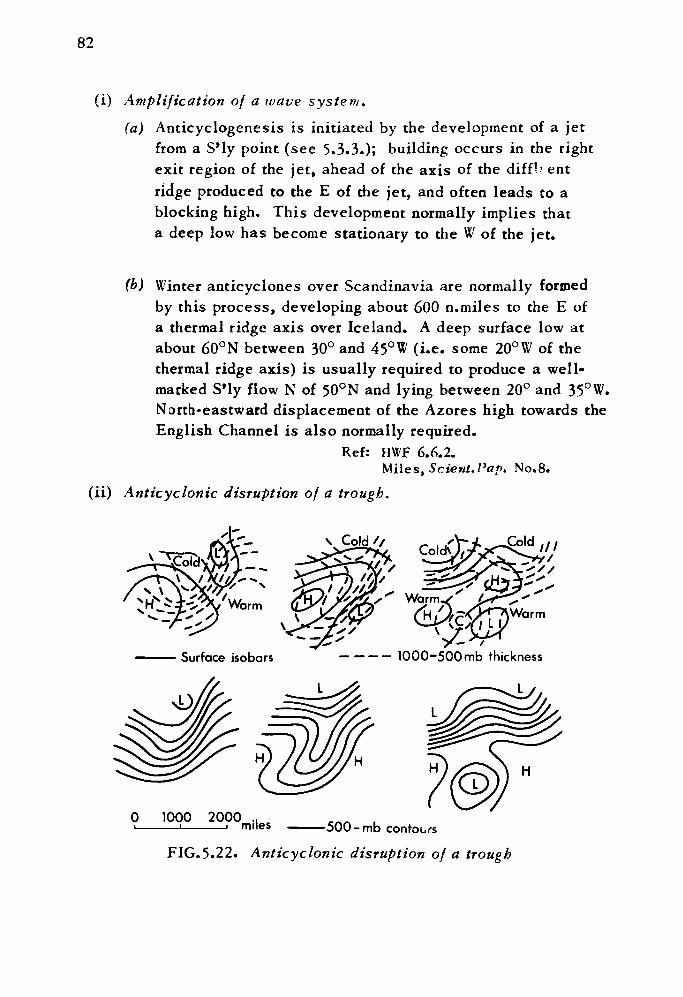
82
(i) Amplification of a wave system.
(a) Anticyclogenesis is initiated by the development of a jet from a S'ly point (see 5.3.3.); building occurs in the right exit region of the jet, ahead of the axis of the difflrent ridge produced to the E of the jet, and often leads to a blocking high. This development normally implies that a deep low has become stationary to the W of the jet.
(b) Winter anticyclones over Scandinavia are normally formed by this process, developing about 600 n.miles to the E of a thermal ridge axis over Iceland. A deep surface low at about 60°N between 30° and 45° W (i.e. some 20° W of the thermal ridge axis) is usually required to produce a well- marked S'ly flow N of 50°N and lying between 20° and 35°W. North-eastward displacement of the Azores high towards the English Channel is also normally required.
Ref: HWF 6.6.2.Miles, Sclent.Pap. No.8.
(ii) Anticyclonic disruption of a trough.
Surface isobars —-- 1000-500mb thickness
L
1000 2000miles
H
-500-mb contours
FIG.5.22. Anticyclonic disruption of a trough
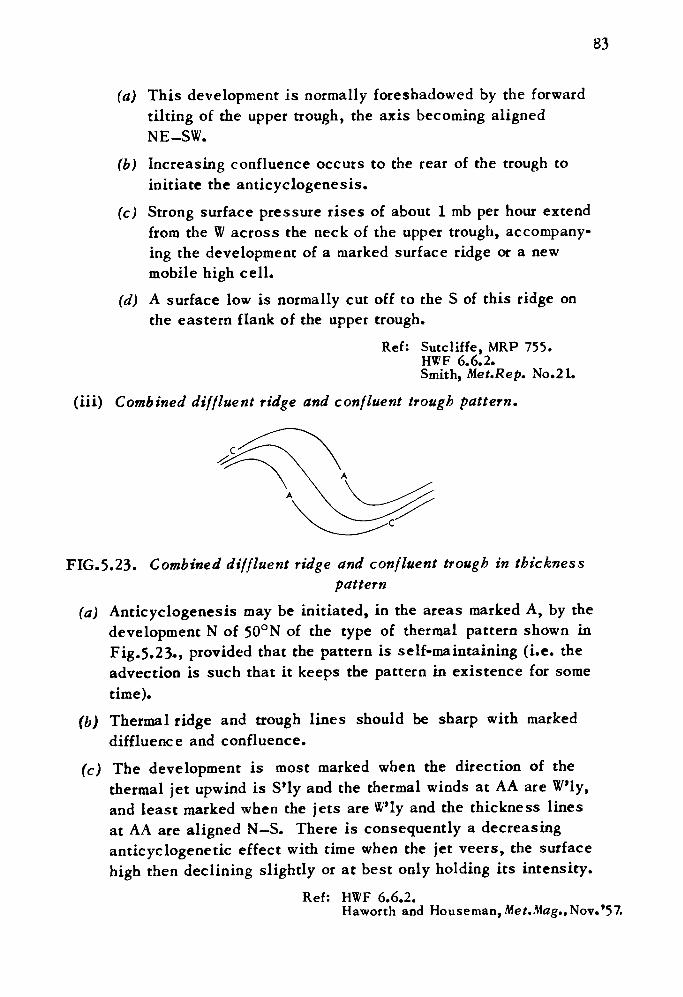
83
(a) This development is normally foreshadowed by the forward tilting of the upper trough, the axis becoming alignedNE-SW.
(b) Increasing confluence occurs to the rear of the trough to initiate the anticyclogenesis.
(c) Strong surface pressure rises of about 1 mb per hour extend from the W across the neck of the upper trough, accompany ing the development of a marked surface ridge or a new mobile high cell.
(d) A surface low is normally cut off to the S of this ridge on the eastern flank of the upper trough.
Ref: Sutcliffe, MRP 755. HWF 6.6.2. Smith, Met.Rep. No.21.
(iii) Combined diffluent ridge and confluent trough pattern.
FIG.5.23. Combined diffluent ridge and confluent trough in thicknesspattern
(a) Anticyclogenesis may be initiated, in the areas marked A, by the development N of 50°N of the type of thermal pattern shown in Fig.5.23-, provided that the pattern is self-maintaining (i.e. the advection is such that it keeps the pattern in existence for some time).
(b) Thermal ridge and trough lines should be sharp with marked diffluence and confluence.
(c) The development is most marked when the direction of the thermal jet upwind is S'ly and the thermal winds at AA are Wly, and least marked when the jets are Wly and the thickness lines at AA are aligned N—S. There is consequently a decreasing anticyclogenetic effect with time when the jet veers, the surface high then declining slightly or at best only holding its intensity.
Ref: HWF 6.6.2.Haworth and Houseman, Met. .Mag.,Nov.'57.
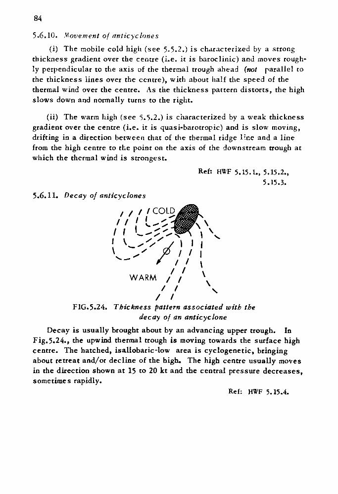
84
5.6.10. Movement of nnticyclones
(i) The mobile cold high (see 5-5.2.) is characterized by a strong thickness gradient over the centre (i.e. it is baroclinic) and moves rough ly perpendicular to the axis of the thermal trough ahead (not parallel to the thickness lines over the centre), with about half the speed of the thermal wind over the centre. As the thickness pattern distorts, the high slows down and normally turns to the right.
(ii) The warm high (see 5.5.2.) is characterized by a weak thickness gradient over the centre (i.e. it is quasi-barotropic) and is slow moving, drifting in a direction between that of the thermal ridge lt.ne and a line from the high centre to the point on the axis of the downstream trough at which the thermal wind is strongest.
Ref: HWF 5.15.1., 5.15.2., 5.15.3.
5.6.11. Decay of anticyclones
FIG.5.24. Thickness pattern associated with the decay of an anticyclone
Decay is usually brought about by an advancing upper trough. In Fig.5.24., the upwind thermal trough is moving towards the surface high centre. The hatched, isallobaric-low area is cyclogenetic, bringing about retreat and/or decline of the high. The high centre usually moves in the direction shown at 15 to 20 kt and the central pressure decreases, sometimes rapidly.
Ref: HWF 5.15.4.
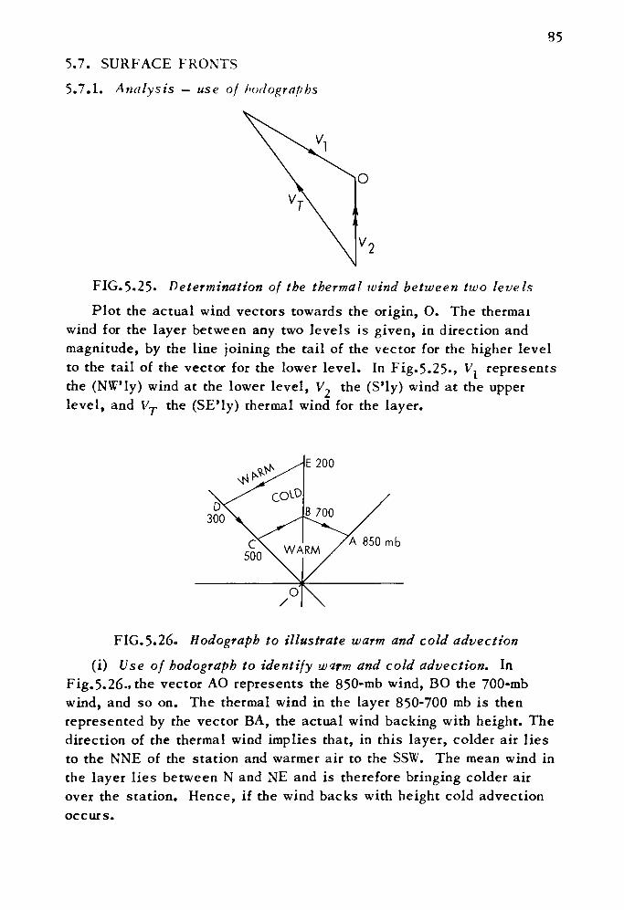
35
5.7. SURFACE FRONTS
5.7.1. Analysis — use of bodographs
FIG.5.25- Determination of the thermal wind between two levels
Plot the actual wind vectors towards the origin, O. The thermal wind for the layer between any two levels is given, in direction and magnitude, by the line joining the tail of the vector for the higher level to the tail of the vector for the lower level. In Fig.5.25-, V, represents the (NW'ly) wind at the lower level, V2 the (S'ly) wind at the upper level, and Vj the (SE'ly) thermal wind for the layer.
E 200
FIG.5.26. Holograph to illustrate warm and cold advection
(i) Use of holograph to identify warm and cold advection. In Fig.5.26-. the vector AO represents the 850-mb wind, BO the 700-mb wind, and so on. The thermal wind in the layer 850-700 mb is then represented by the vector BA, the actual wind backing with height. The direction of the thermal wind implies that, in this layer, colder air lies to the NNE of the station and warmer air to the SSW. The mean wind in the layer lies between N and NE and is therefore bringing colder air over the station. Hence, if the wind backs with height cold advection occurs.
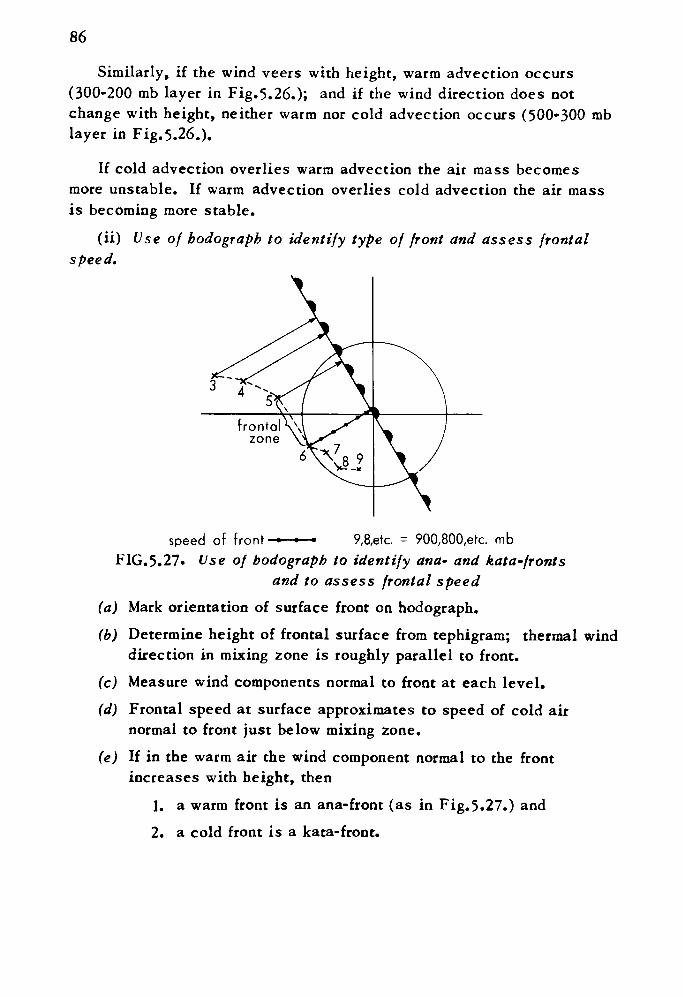
86
Similarly, if the wind veers with height, warm advection occurs (300-200 mb layer in Fig.5.26.); and if the wind direction does not change with height, neither warm nor cold advection occurs (500-300 mb layer in Fig.5.26.).
If cold advection overlies warm advection the air mass becomes more unstable. If warm advection overlies cold advection the air mass is becoming more stable.
(ii) Vse of bodograph to identify type of front and assess frontal speed.
speed of front • 9,8,etc. = 900,800,etc. mbFIG.5.27. Use of bodograph to identify ana~ and kata-fronts
and to assess frontal speed(a) Mark orientation of surface front on hodograph.
(b) Determine height of frontal surface from tephigram; thermal wind direction in mixing zone is roughly parallel to front.
(c) Measure wind components normal to front at each level.(d) Frontal speed at surface approximates to speed of cold air
normal to front just below mixing zone.
(e) If in the warm air the wind component normal to the front increases with height, then
1. a warm front is an ana-front (as in Fig.5.27.) and
2. a cold front is a kata-front.
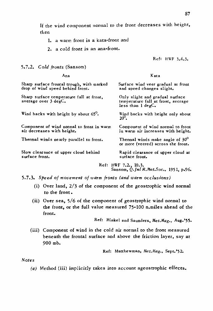
37
If the wind component normal to the front decreases with height, then
1. a warm front is a kata-front and
2. a cold front is an ana-front.
Ref: HWF 3.4.3.
5.7.2. Cold fronts (Sansom)
Ana Kata
Sharp surface frontal trough, with marked Surface wind veer gradual at front drop of wind speed behind front. and speed changes slight.
Sharp surface temperature fall at front, Only slight and gradual surface average over 3 degC. temperature fall at front, average
less than 1 degC.
Wind backs with height by about 65°. Wind backs with height only about20°.
Component of wind normal to front in warm Component of wind normal to front air decreases with height. in warm air increases with height.
Thermal winds nearly parallel to front. Thermal winds make angle of 30°or more (veered) across the front.
Slow clearance of upper cloud behind Rapid clearance of upper cloud at surface front. surface front.
Ref: HWF 7.2., 10.3.Sansom, Q.Jnl R.Met.Soc., 1951, p.96.
5.7.3. Speed of movement of warm fronts (and warm occlusions)
(i) Over land, 2/3 of the component of the geostrophic wind normal to the front.
(ii) Over sea, 5/6 of the component of geostrophic wind normal to the front, or the full value measured 75-100 n.miles ahead of the front.
Ref: Hinkel and Saunders, Met.Mag., Aug.'55.
(iii) Component of wind in the cold air normal to the front measured beneath the frontal surface and above the friction layer, say at 900 mb.
Ref: Matthewman, Met.Mag., Sept.'5 2.
Notes
(a) Method (iii) implicitly takes into account ageostrophic effects.
88
(b) Methods (i) and (ii) do not take into account ageostrophic effects in the cold air. Approximate quantitative corrections can be made for curvature and for pressure changes (see 4,3« and 4.2.(iii)). 5.7.4. Movement of cold fronts (and cold occlusions)
Full component of geostrophic wind normal to the front. Notes
(a) Corrections for curvature and pressure changes should be applied (see 4.3. and 4.2.(iii)). This is particularly important when there is a strong isallobaric gradient across the front.
(b) Supergeostrophic motion may occur, notably in summer at the end of hot spells, where the fronts are upper fronts in character, the pseudo- surface boundary extending down to the surface in descending squalls.
Ref: HWF 6.7.3.
CHAPTER 6. PRECIPITATION
6.1. GENERAL PRINCIPLESIn order to produce precipitation, there must be both sufficient ascent
and sufficient moisture.6.1.1. Dynamical ascent: use of contour/thickness charts
Areas in which large-scale dynamical ascent (frontal or non-frontal) will occur, may broadly be identified with C (cyclonic) development areas on contour or thickness charts (see 5*6.1. and 5.6.8.).
Dynamical ascent and descent also exert an influence on convective precipitation; if the flow at both lower and upper tropospheric levels shows cyclonic vorticity the chance of showers is enhanced, whereas anticyclonic vorticity is associated with less shower activity. If the air mass is one in which shower development is expected, this will be stimulated in the region immediately ahead of an upper trough, but the passage of the upper trough axis will usually lead to a marked reduction of both the frequency and the intensity of the showers, even when the surface flow is unchanged.
Ref: HWF 16.7.3.
6.1.2. Moisture: use of tephigrams and 700-mb dew-point depression charts
Detailed information on the vertical distribution of moisture can only be determined from tephigrams; from these, vertical cross-sections along particular lines can be constructed, and are sometimes useful.
Although the moisture pattern at 700 mb is not necessarily represen tative of that at nearby levels, 700-mb dew-point depression charts are often useful as an indication of available moisture at medium-cloud levels. Areas of moist air indicated by isopleths on these charts may be moved with the 700-mb winds, but patterns will be modified by vertical motion; areas of moist air are maintained by ascent, but descending air will lead to drying out. It can sometimes be foreseen that 700-mb advection will bring an area of moist air into a region of marked dynami cal ascent; this will lead to development or intensification of precipi tation.
89
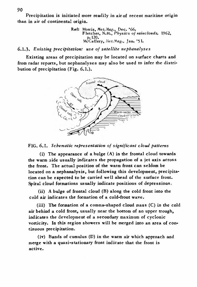
90Precipitation is initiated more readily in air of recent maritime origin
than in air of continental origin.
Ref: Morris, Met.Mag.. Dec. '66.Fletcher, N.H., Physics of rainclouds, 1962,
p. 120. McCaffery, Met.Mag., Jan. '51.
6.1.3. Existing precipitation: use of satellite nephanalyses
Existing areas of precipitation may be located on surface charts and from radar reports, but nephanalyses may also be used to infer the distri bution of precipitation (Fig. 6.1.).
FIG. 6.1. Schematic representation of significant cloud patterns
(i) The appearance of a bulge (A) in the frontal cloud towards the warm side usually indicates the propagation of a jet axis across the front. The actual position of the warm front can seldom be located on a nephanalysis, but following this development, precipita tion can be expected to be carried well ahead of the surface front. Spiral cloud formations usually indicate positions of depressions.
(ii) A bulge of frontal cloud (B) along the cold front into the cold air indicates the formation of a cold-front wave.
(iii) The formation of a comma-shaped cloud mass (C) in the cold air behind a cold front, usually near the bottom of an upper trough, indicates the development of a secondary maximum of cyclonic vorticity. In this region showers will be merged into an area of con tinuous precipitation.
(iv) Bands of cumulus (D) in the warm air which approach and merge with a quasi-stationary front indicate that the front is active.
91(v) Reports of 'open cells' imply the presence of deep convection
and therefore showers. 'Closed cells' imply convection of limited depth and far less shower activity.
Ref: WMO Tech. Note. No. 75
6.2. FRONTAL PRECIPITATION
6.2.1. General approach
(i) Use thickness pattern to check surface analysis (amending the latter if necessary), and to identify areas of frontogenesis and frontolysis. Frontogenesis usually leads to active ascent of the warm air and hence precipitation before typical frontal characteristics become apparent on the surface chart.
(ii) Examine 500-or 300-mb contours in conjunction with surface chart, and compare speeds of movement of corresponding surface and upper air features during the previous 24 h. Fronts likely to become assoc iated with areas of dynamical ascent will intensify (e.g. upper trough catches up surface front, frontal wave reaches left exit or right entrance region of a jet); the converse also holds (e.g. anticyclonic disruption). In assessing the implications of an upper flow pattern, development of the pattern itself must be taken into account as well as advection (e.g. meridional trough extension; buckling of zonal flow leading to jet- stream development).
(iii) Use tephigrams and 700-mb dew-point depression charts to check on the maintenance of a supply of moisture. Wet'bulb potential temperatures may sometimes reveal useful information; in particular high values indicate large amounts of moisture (e.g. ahead of ex-tropic^t hurricanes).
(iv) Use surface charts, nephana/yses and radar reports to assess latest pattern of precipitation. Developmental changes indicated by (i)-(iii) should be applied.
(v) Use hodographs (see 5.7.1.) to infer the relative vertical motion at a front, and so identify those fronts which possess marked ana or kata characteristics.
(vi) Consider orographic effects, including the possibility of the release of potential instability. The average rate of frontal rainfall over level country in the British Isles is about 1 to 2 mm/h, but the rate is probably greater by a factor of two to four over high ground. Orographic effects are most marked, leading to large orographic rainfall (e.g. 50 mm in 24 h over Uelsh Mountains) when
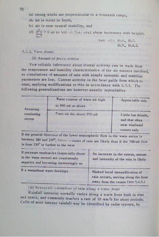
93
hourly rainfall charts, or sometimes by the mesoscale tendency field. Such cells appear to have a typical life of 6 to 12h, so that if identified early in their life they can be followed and forecast. The cells usually behave like warm-front waves, moving along the front away from the low centre; alternatively the 700-mb flow often gives a rough indication of movement.
Ref: HWF 10.2., 16.5.Wallington, Weather, June '63.Jones, Met. Mag., Nov. '66.
6.2.3. Cold fronts
(i) Cold ana- aad kata-fronts (see 5.7.2.) have markedly different characteristics.
Cold ana-fronts Cold kata-fronts
Frequency in British Isles
Dec. to May (29% unclassified) June to Nov. (19% unclassified)
Wave developmentActivityPrecipitation on frontPrecipitation behind front
54% 8%
LikelyStrong
Fairly heavy rainLight (occasionally moderate) rain extends about 100 n. miles behind surface front, with rain continuing almost to upper cloud edge
17%73%
UnlikelyWeak
Little or noneVery little rain behind surface front
(ii) Mesoscale variations of rain along a cold front
The amount of rainfall along a particular cold front is character istically extremely variable both in time and in space; rainfall rates of as much as 20 mm/h probably occut quite frequently for periods of a few minutes. Areas of more intense rainfall are sometimes associated with embedded convective cells, which may be detected by radar reports. On cold-ana fronts, local intensification of rainfall is also caused by minor waves which may be identified on nephanalyses or by the mesoscale tendency field. These areas of intensification behave like normal cold-front waves, and move along the front towards
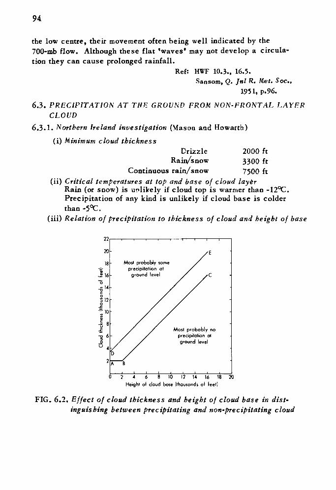
94
the low centre, their movement often being well indicated by the 700-mb flow. Although these flat 'waves' may not develop a circula tion they can cause prolonged rainfall.
Ref: HWF 10.3., 16.5.Sansom, Q. Jnl R. Met. Soc.,
1951, p.96.
6.3. PRECIPITATION AT THE GROUND FROM NON-FRONTAL LAYFR CLOUD
6.3.1. Northern Ireland investigation (Mason and Howarth)
(i) Minimum cloud thicknessDrizzle 2000 ft
Rain/snow 3300 ftContinuous rain/snow 7500 ft
(ii) Critical temperatures at top and base of cloud layerRain (or snow) is unlikely if cloud top is warmer than -12°C. Precipitation of any kind is unlikely if cloud base is colder than -5^.
(iii) Relation of precipitation to thickness of cloud and height of base
22
20
18
J>16"o
-B Mc O312 o
Most probably someprecipitation at
ground level
Most probably no precipitation at ground level
2 4 6 8 10 12 14 16 18 20 Height of cloud base (thousands of feet)
FIG. 6.2. Effect of cloud thickness and height of cloud base in dist inguishing between precipitating and non-precipitating cloud
95 Notes
(a) When a point falls between the lines ABC and DE in Fii/. 6.2. judgement must be exercised.
(b) The investigation excluded all cases when cumulus cloud or showers were reported; the results must therefore be applied with discretion when a cloud layer is convectively maintained (e.g. over the North Sea in winter).
Ref: Mason and Howarth, Q. Jnl R. Met. Soc.. 1952, p.226.
6.3.2. Met.R.F. investigation over central England (Stewart)
(i) Clouds with bases above the 0°C isotherm level
Height of cloud base above 0°C level Cloud thickness Probability of ppn
reaching ground
Less than 3300 ft More than 3300 ft
More than 6600 ft All values
90%5%
(ii) Clouds with bases below 0°C isotherm levelMinimum thickness for: any precipitation 1320ft
slight rain 3300 ftmoderate rain 9900 ft
NoteBased on 8 years of observations.
Ref: Stewart, Q. Jnl R. Met. Soc., 1964, p.287.
6.4. CONVECTIVE PRECIPITATION 6.4.1. General approach
(i) OccurrenceThe likelihood, frequency and intensity of convective
precipitation are increased by:(a) Dynamical ascent (see 6.1.1.)(b) Adequate moisture (see 6.1.2., 6.4.7. and 6.4.8.)(c) Appearance of 'open cell' cloud structure (see 6.1.3.)
. (d) High instability indices (see 6.4.7.) (e) Low cloud-top temperatures (see 6.4.2.) (/) Large depth of convection (see 6.4.3., 6.4.6., 6.4.7. and
6.4.8.)
(g) Small vertical wind shear (see 6.4.4. but also 6.4.8.) (b) High cloud-base temperatures (see 6.4.8.)
(ii) Life and direction of movementThe typical life cycle of a convection cell (i.e. growth, shower
production and decay) is completed within about one hour. Individual showers can best be followed by radar, but extrapolations should not be made for oeriods in excess of 1 h; the best guide for the movement of air-mass showers during this period is the 700-mb wind.
Note
These remarks do not apply to severe storms (see 6.4.8.).
6.4.2. Cloud-top temperatures
For showers by the Oergeron /Findeisen process:Cloud-top temperature Shower probability
degrees Celsius
0 to —12 Slight possibility-12 to-40 Likely Below —40 Almost certain
Ref: HWF 16.7.3.
6.4.3. Cloud depth(i) Showers rarely occur unless the cloud depth as calculated by
the parcel method exceeds 150 mb.(ii) Showers from quite shallow convective cloud (say 5000 ft)
are not frequent, but those that do occur are most common near windward coasts in the early or mid-morning; in these cases, larger clouds formed later in the day sometimes fail to produce showers.
Note
Investigation was carried out using data for southern England.
Ref: HWF 16.7.3.1.
6.4.4. TI feet of vertical win:! shearOnly scattered light showers occur if the mean vertical wind
shear from the ground to the expected cloud top exceeds 3 kt/1000 ft.
(a) Applies to air-mass showers only and not to those initiated by dynamical uplift.
(b) Does not apply to severe 1 >cal storms for whicli vertical shear is necessary (6.4.R.)
Ref: HVfF 16.7.3.2.
6.4.5. Effects of local topography
(i) Areas over, and immediately downwind of southward faring slopes are preferred regions for shower development.
(ii) The ascent of moist air at a sea-breeze front may initiate showers. If two sea-breeze fronts approach one another, the shower likelihood is increased in the region of convergence.
(iii) When a moderate or strong airflow crosses hilly country, standing-wave conditions may develop (see 8.4.3.). Areas of persistent downcurrents may then remain shower-free all day, whilst areas of persistent upcurrents have frequent showers.
Ref: HWF 16.8.2.Findlater, Met. Mag., Mar. '^4 •Wosler, Davis and Booker, Met. Abstract
No. 212.
5.4.6. //^/'/(excluding soft hail)(i) None of the known objective techniques for local forecasting
of hail has yet been found suitable for use in the U.K.
(ii) An empirical rule suggest that hail is likely when the parcel method indicates cloud tops of at least 15 000 ft, with the path and environment curves at least 5 degC apart throughout most of the cloud depth.
(iii) As hail is often associated with thunderstorms, it is customary to forecast hail whenever thunder is forecast. There is, however, evidence to suggest that damaging large hail is unlikely if there is frequent lightning.
Ref: FTBM No. 1.Sansom, Weather, Sept. '66.
98
6.4.7. Thunderstorms
(i) Instability indices Boyden Index
/ = Z - T - 200,where Z = 1000—700 mb thickness in decametres
T = 700-mb temperature in °C.Notes
(a) Index isopleths can be advected with 700-mh winds,(b) Threshold value is around 94/95«
Rackliff IndexT = _,.. 500'
where Q WQQQ = 900-mb wet-bulb potential temperature in °C,500-mb temperature in °C.
Note
Threshold value is around 29/30.
Modified Jefferson Index
Tmj = L6^u#00 ~ T500 " ^T dJOO ~~ 8' where Tjjnn = 700-mb dew-point in °C.
Notes
(a) OyjQcn may be used instead of ft^ggo a°d has little effect on the result provided there is no inversion between 350 and 900 mb.
(b) Threshold value is around 26/2?.Ref: Boyden, Met. Mag., July '63
Rackliff, Met. Mag., May '62 Jefferson, Met. Mag., Oct. '63 FTBM No. 14.
The most successful indices for thunderstorm forecasting in the U.K. appear to be
(a) Boyden Index — especially for frontal and trough situations, and
(b) Rackliff and modified Jefferson — especially for air-mass convection.
99Note
Trials suggest that a subjective assessment using the indices gives a better result than the use of indices alone,
(ii) General considerationsConvection may be released by surface heating, convergence, or
forced ascent. The possibility of release of potential (convective) instability must also be considered, particularly in frontal and trough situations.
(a) Depth of convection:Cloud tops less than 13 000 ft Thunder most unlikely Depth of convection 400 to 500 mb Thunder probable Depth of convection over 500 mb At least 50% of showers
accompanied by thunder
When assessing likely depth of convection, subjective allow ance must be made for subsidence and for advective temperature changes.
(b) For general thunderstorm development, the air must be moist in depth; dry air aloft implies only isolated storms, but with adequate moisture thunderstorms can readily occur with only slight insta bility through sufficient depth.(c) SFLOC reports are most valuable.
Ref: HWF 16.7.5.16.7.3.1.
FTBM Nos 8 and 14.
6.4.8. Severe Local Storms
The term Severe Local Storm has a special connotation; it refers only to an intense convection cloud system which has become self- maintaining. Severe Local Storms normally develop only in the particular circumstances outlined below and, once developed, have a characteristic behaviour which is quite distinct from that of normal convective storms (including those which are described and coded as severe).
(i) Formation normally requires:
(a) A supply of warm moist air at low levels, i.e. high values of surface wet-bulb potential temperature (Ow ), typically about 20°C.
100
(b) Great depth of instability.
(c) Great buoyancy, indicated by a large excess of BW over the saturation wet-bulb potential temperature (6 ) in
the middle and upper troposphere.
(d) Vertical wind shear, typically a veer with height throughout the convective layer. The convective layer is the entire troposphere for Severe Local Storms, and shear between the ground and the 500-mb level is usually in the range 30-60 kt.
(e) Trigger action, namely day-time surface heating, low- level convergence, or orographic uplift.
Note
These requirements are most likely to be met in the S'ly flow ahead
of a major trough. Northward advection, at a height of 3000-7000 ft, of
air warmed over Spain can then form a lid to small-scale surface convec
tion such that low-level moisture is confined beneath this lid and high
buoyancy can develop. Advective cooling aloft is meanwhile aided by
large-scale ascent.
(ii) Characteristics(a) Ordinary non-severe showers and thunderstorms usually
consist of aggregates of convective cells each of which goes through three stages of evolution (Byers and B rah am): (1) the cumulus stage (updraught alone), (2) the mature stage (updraught and downdraught together), and (3) the dissipating stage (downdraught alone). Bowever, when a thunderstorm develops into a Severe Local Storm the ordinary mature stage, instead of lasting for the usual 15 to 30 min, evolves into a 'severe mature' stage that can persist for periods of up to several hours.
Ref: Byers and Braham, Thunderstorm Rpt, Washington, 194«.
(b) Whereas normal convective systems move roughly with the mid-tropospheric winds, once the severe mature stage is
reached movement is some 20° either to the right of and slower than, or to the left of and faster than, the mid- trapospheric winds, i.e. progression is developmental not
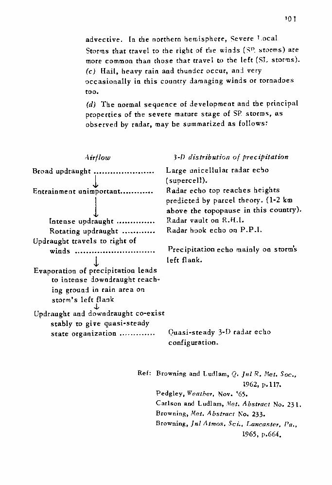
'01
advective. In the northern hemisphere, Severe T .ocal
Storms that travel to the right of the winds (S p. storms) are more common than those that travel to the left (ST. storms).(c) Hail, heavy rain and thunder occur, and very occasionally in this country damaging winds or tornadoes too.
(d) The normal sequence of development and the principal properties of the severe mature stage of SP storms, as observed by radar, may be summarized as follows:
Airflow 3-0 distribution of precipitation
Broad updraught ...................... Large unicellular radar echoI (supercell).
Entrainment unimportant............ Radar echo top reaches heightsI predicted by parcel theory. (1-2 km I above the topopause in this country).
Intense updraught .............. Radar vault on R.H.I.Rotating updraught ............ Radar hook echo on P.P.I.
Updraught travels to right ofwinds ............................. Precipitation echo mainly on storms
^ left flank. Evaporation of precipitation leads
to intense downdraught reach ing ground in rain area on storm's left flank
± Updraught and downdraught co-exist
stably to give quasi-steadystate organization ............. Quasi-steady 3-D radar echo
c onf igur ation.
Ref: Browning and Ludlam, Q. Jnl R. Net. Soc.,
1962, p. 117.Pedgley, Weather. Nov. '65. Carlson and Ludlam, Met. Abstract No. 231. Browning, Met. Abstract No. 233. Browning, Jnl Atmos. Set., Lancaster, Pa.,
1965, p.664.
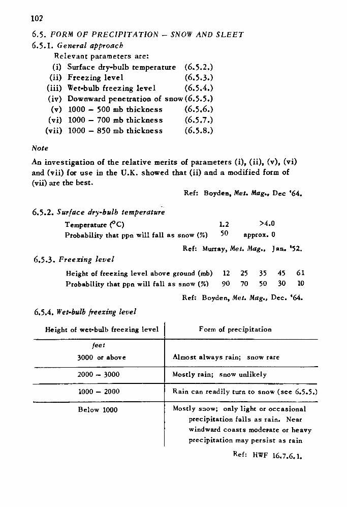
102
6.5. FORM OF PRECIPITATION - SNOW AND SLEET6.5.1. General approach
Relevant parameters are:(i) Surface dry-bulb temperature (6.5.2.)
(ii) Freezing level (6.5.3.)(iii) Wet-bulb freezing level (6.5.4.)(iv) Downward penetration of snow (6.5.5.)(v) 1000 - 500 mb thickness (6.5.6.)
(vi) 1000 - 700 mb thickness (6.5.7.)(vii) 1000 - 850 mb thickness (6.5.8.)
Note
An investigation of the relative merits of parameters (i), (ii), (v), (vi) and (vii) for use in the U.K. showed that (ii) and a modified form of (vii) are the best.
Ref: Boyden, Met. Mag., Dec '64.
6.5.2. Surface dry-bulb temperatureTemperature (°C) 1.2 >4.0 Probability that ppn will fall as snow (%) 50 appro*. 0
Ref: Murray, Met. Mag., Jan. '52.6.5.3. Freezing level
Height of freezing level above ground (mb) 12 25 35 45 61 Probability that ppn will fall as snow (%) 90 70 50 30 10
Ref: Boyden, Met. Mag., Dec. '64.
6.5.4. Wet-bulb freezing level
Height of wet-bulb freezing level Form of precipitation
feet
3000 or above Almost always rain; snow rare
2000 - 3000 Mostly rain; snow unlikely
1000 - 2000 Rain can readily turn to snow (see 6.5.5.)
Below 1000 Mostly snow; only light or occasional precipitation falls as rain. Near windward coasts moderate or heavy precipitation may persist as rain
Ref: HWF 16.7.6.1.
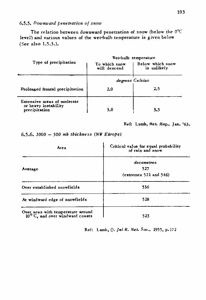
103
6.5.5. Downward penetration of snow
The relation between downward penetration of snow (below the 0°C level) and various values of the wet-bulb temperature is given below (See also 1.5.3.).
Type of precipitationWet-bulb temperature
To which snow will descend
Below which snow is unlikely
Prolonged frontal precipitation
degrees Celsius
2.0 2.5
Extensive areas of moderate or heavy instability precipitation 3.0 3.5
Ref: Lumb, Met. Mag., Jan. '63.
6.5.6. 1000 - 500 mb thickness (NW Eitrope)
Area Critical value for equal probability of rain and snow
Average
Over established snowfields
At windward edge of snowfields
Over seas with temperature around 10° C, and over windward coasts
decametres527
(extremes 521 and 546)
536
528
523
Ref: Lamb, Q. Jnl R. Met. Soc., 1955, p. 172
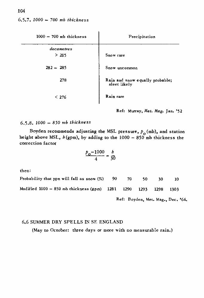
104
6.5.7. 1000 - 700 mb thickness
1000 - 700 mb thickness Precipitation
decametres> 285
282 - 285
278
< 276
Snow rare
Snow uncommon
Rain and snow equally probable; sleet likely
Rain rare
Ref: Murray, Met. Mag. Jan. '52
6.5.8. 1000 - 850 mb thickness
Boyden recommends adjusting the MSL pressure, fto (mb), and station height above MSL, A(gpm), by adding to the 1000 - 850 mb thickness the correction factor
- 1000
then:
Probability that ppn will fall as snow (%) 90 70 50 30 10
Modified 1000 - 850 mb thickness (gpm) 1281 1290 1293 1298 1303
Ref: Boyden, Met. Mag., Dec. '64.
606 SUMMER DRY SPELLS IN SE ENGLAND
(May to October: three days or more with no measurable rain.)
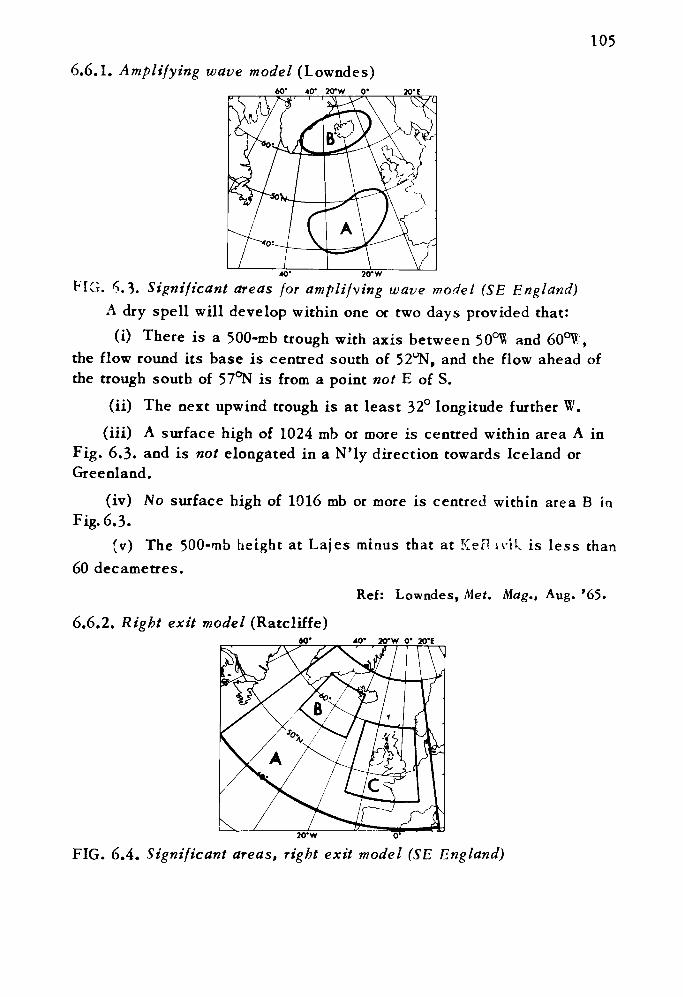
105
6.6.1. Amplifying wave model (Lowndes)AO* 40" ao*w 0*
20'W
FIG. ^.3. Significant areas for amplifying wave model (SE England) A dry spell will develop within one or two days provided that:
(i) There is a 500-mb trough with axis between 50°W and 60°V, the flow round its base is centred south of 52^, and the flow ahead of the trough south of 57°N is from a point not E of S.
(ii) The next upwind trough is at least 32° longitude further W.(iii) A surface high of 1024 mb or more is centred within area A in
Fig. 6.3. and is not elongated in a N'ly direction towards Iceland or Greenland.
(iv) No surface high of 1016 mb or more is centred within area B in Fig. 6.3.
(v) The 500-mb height at Lajes minus that at KefliviL is less than 60 decametres.
Ref: Lowndes, Met. Mag., Aug. '65.
6.6.2. Right exit model (Ratcliffe)40* ___ 40"
20'W
FIG. 6.4. Significant areas, right exit model (SE England)
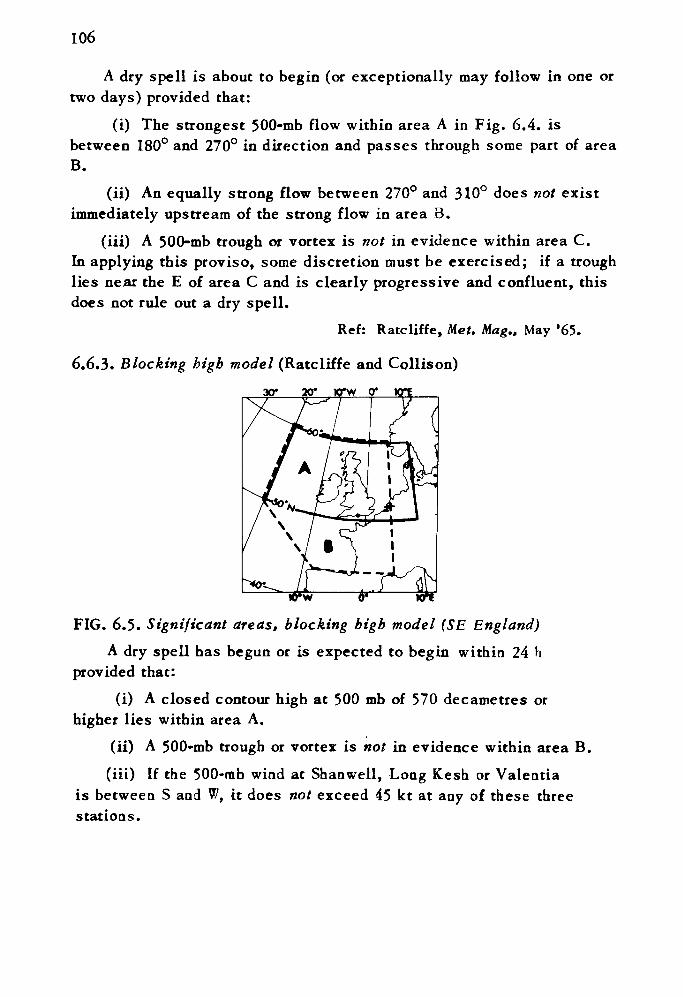
106
A dry spell is about to begin (or exceptionally may follow in one or two days) provided that:
(i) The strongest 500-mb flow within area A in Fig. 6.4. is between 180° and 270° in direction and passes through some part of area B.
(ii) An equally strong flow between 270° and 310° does not exist immediately upstream of the strong flow in area B.
(iii) A 500-mb trough or vortex is not in evidence within area C. In applying this proviso, some discretion must be exercised; if a trough lies near the E of area C and is clearly progressive and confluent, this does not rule out a dry spell.
Ref: Ratcliffe, Met. Mag.. May '65.
6.6.3. Blocking high model (Ratcliffe and Collison)
FIG. 6.5. Significant areas, blocking high model (SE England)
A dry spell has begun or is expected to begin within 24 h provided that:
(i) A closed contour high at 500 mb of 570 decametres or higher lies within area A.
(ii) A 500-mb trough or vortex is not in evidence within area B.
(iii) If the 500-mb wind at Shaawell, Long Kesh or Valentia is between S and W, it does not exceed 45 kt at any of these three stations.
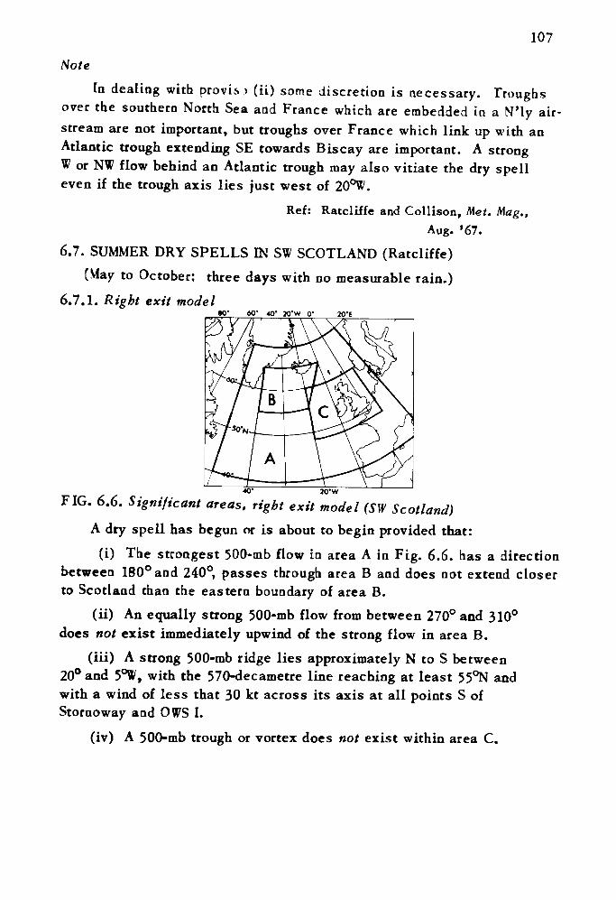
107
Note
In dealing with provis > (ii) some discretion is necessary. Troughs over the southern North Sea and France which are embedded in a N'ly air- stream are not important, but troughs over France which link up with an Atlantic trough extending SE towards Biscay are important. A strong W or NW flow behind an Atlantic trough may also vitiate the dry spell even if the trough axis lies just west of 20°W.
Ref: Ratcliffe and Collison, Met. Mag.,Aug. '67.
6.7. SUMMER DRY SPELLS IN SW SCOTLAND (Ratcliffe) (May to October: three days with no measurable rain.)
6.7.1. Right exit model60' 40' 30'W 0' 20'E
20'W
FIG. 6.6. Significant areas, right exit model (SW Scotland) A dry spell has begun or is about to begin provided that:
(i) The strongest 500-mb flow in area A in Fig. 6.6. has a direction betweea 180° and 240°, passes through area B and does not extend closer to Scotland than the eastern boundary of area B.
(ii) An equally strong 500-mb flow from between 270° and 310° does not exist immediately upwind of the strong flow in area B.
(iii) A strong 500-mb ridge lies approximately N to S between 20° and 5°W, with the 570-decametre line reaching at least 55°N and with a wind of less that 30 kt across its axis at all points S of Stornoway and OWS I.
(iv) A 500-mb trough or vortex does not exist within area C.
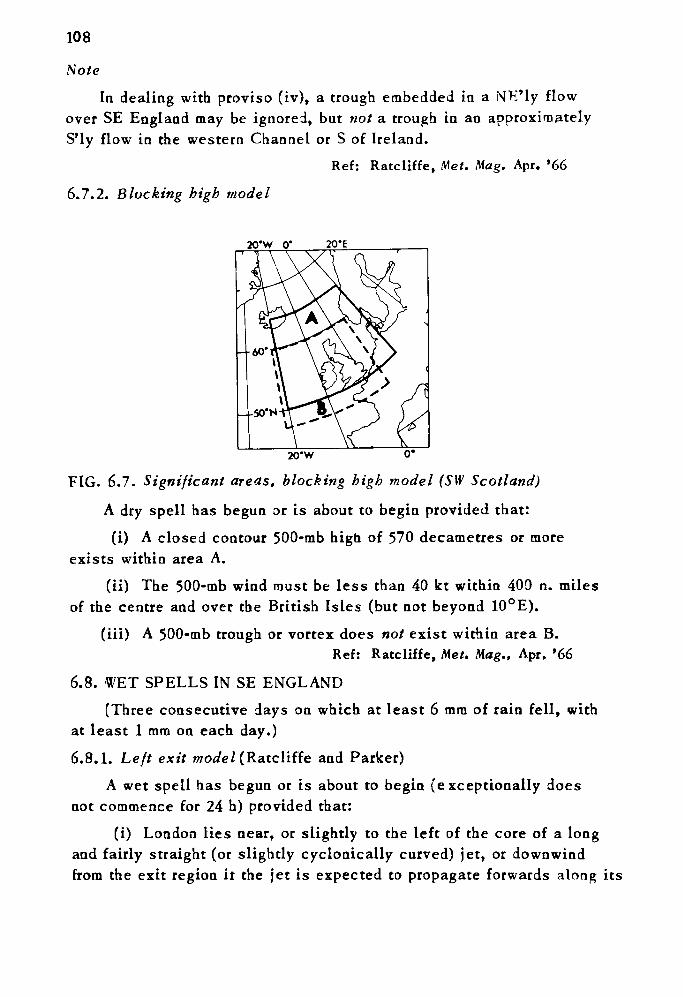
108
Note
In dealing with proviso (iv), a trough embedded in a NE'ly flow
over SE England may be ignored, but not a trough in an approximately S'ly flow in the western Channel or S of Ireland.
6.7.2. Blocking high modelRef: Ratcliffe, Met. Mag. Apr. '66
20*w o* 20*E
20'W 0*
FIG. 6.7. Significant areas, blocking high model (SW Scotland)
A dry spell has begun or is about to begin provided that:
(i) A closed contour 500-mb high of 570 decametres or more exists within area A.
(ii) The 500-mb wind must be less than 40 kt within 400 n. miles of the centre and over the British Isles (but not beyond 10°E).
(iii) A 500-mb trough or vortex does not exist within area B.Ref: Ratcliffe, Met. Mag., Apr. »66
6.8. WET SPELLS IN SE ENGLAND
(Three consecutive days on which at least 6 mm of rain fell, with at least 1 mm on each day.)
6.8.1. Left exit mode I (Ratcliffe and Parker)
A wet spell has begun or is about to begin (exceptionally does not commence for 24 h) provided that:
(i) London lies near, or slightly to the left of the core of a long and fairly straight (or slightly cyclonically curved) jet, or downwind
from the exit region it the jet is expected to propagate forwards along its
109
path.
(ii) The jet is (normally) the strongest flow in the area bounded by 40°N 70°N 10°E 60°W and is about 1000 n. miles in length, with the greater part W of 10°W.
(iii) There is no 500-mb ridge over the British Isles, and no closed 500-mb vortex over Iberia.Note
Particular care must be exercised when a 500-mb trough exists between 50°W and 60°W (cf. 6.6.1.) Provided such a trough is not well developed, and a further trough exists within 40° longitude upwind, the wet spell may be forecast when the three criteria above are satisfied; but if the trough at 50°W to 60°W is well developed, a wet spell should be forecast only if there is no indication of backing upper flow over the E Atlantic which could lead to ridge development over Britain.
Ref: Ratcliffe and Parker, Met. Mag., Jan '68.
6.8.2. Trough model (Lowndes)The model is based on the likelihood that wet spells occur on the
forward side of upper troughs. Criteria, however, vary from season to season. Full details are given in the original article.
Ref: Lowndes, Met. Mag., Oct. '62.
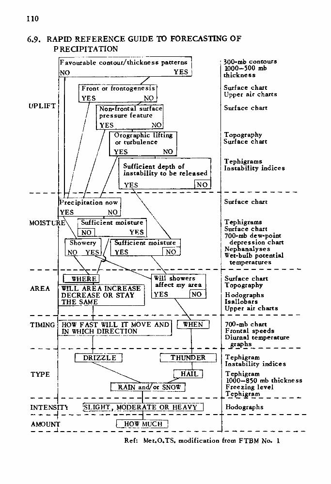
110
6.9. RAPID REFERENCE GUIDE TO FORECASTING OF PRECIPITATION
UPLIFT
Favourable contour/thickness patterns NO YES
Z
I
Front or frontogenesis YES NO
Non-frontal surface pressure featureYES NO
Orographic lifting or turbulenceYES NO
Sufficient depth of instability to be released
YES NO
300-mb contours 1000-500 mb thickness
Surface chart Upper air charts
Surface chart
Topography Surface chart
Tephigrams Instability indices
Precipitation now YES NO
MOISTURE i Sufficient moisture"NO! YES
Sufficient moistureYES JNO
Surface chart
Tephigrams Surface chart 700-mb dew-point
depression chart Nephanalyses Wet-bulb potential
temperatures
AREA WILL AREA INCREASE DECREASE OR STAY THE SAME
Will showers affect my areaYES [NO"
Surface chart TopographyHodographs Isallobars Upper air charts
TIMING HOW FAST WILL IT MOVE AND IN WHICH DIRECTION
WHEN
RAIN and/or SNOW
700-mb chart Frontal speeds Diurnal temperature
graphs
TYPE
INTENSITY--H--AMOUNT
ISLIGHT. MODERATE OR HEAVY 1
Tephigram Instability indicesTephigram1000-850 mb thickness Freezing level Tephigrarn_ _ _ _ _
Hodographs
HOW MUCH!Ref: Met.O.TS. modification from FTBM No. 1
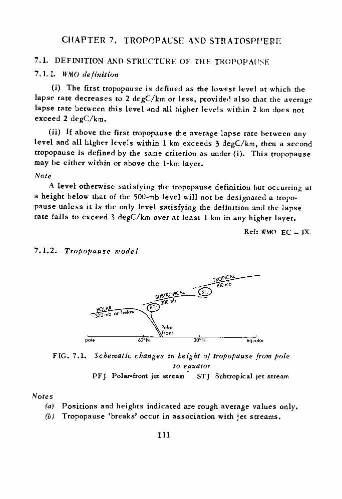
CHAPTER 7. TROPOPAUSE AND STRATOSPHERE
7.1. DEFINITION AND STRUCTURE OF THE TROPOPAUSE 7.. 1.1. WMO definition
(i) The first tropopause is defined as the lowest level at which the lapse rate decreases to 2 degC/km or less, provided also that the average lapse rate between this level and all higher levels within 2 km does not exceed 2 degC/km.
(ii) If above the first tropopause the average lapse rate between any level and all higher levels within 1 km exceeds 3 degC/km, then a second tropopause is defined by the same criterion as under (i). This tropopause may be either within or above the 1-kir. layer.Note
A level otherwise satisfying the tropopause definition but occurring at a height below that of the 500-mb level will not be designated a tropo pause unless it is the only level satisfying the definition and the lapse rate fails to exceed 3 degC/km over at least 1 km in any higher layer.
Ref: WMO EC - IX.
7.1.2. Tropopause model
60°N 30°N equator
FIG. 7.1. Schematic changes in height of tropopause front poleto equator
PFJ Polar-front jet stream STJ Subtropical jet stream
Notes(a) Positions and heights indicated are rough average values only.(b) Tropopause 'breaks' occur in association with jet streams.
Ill
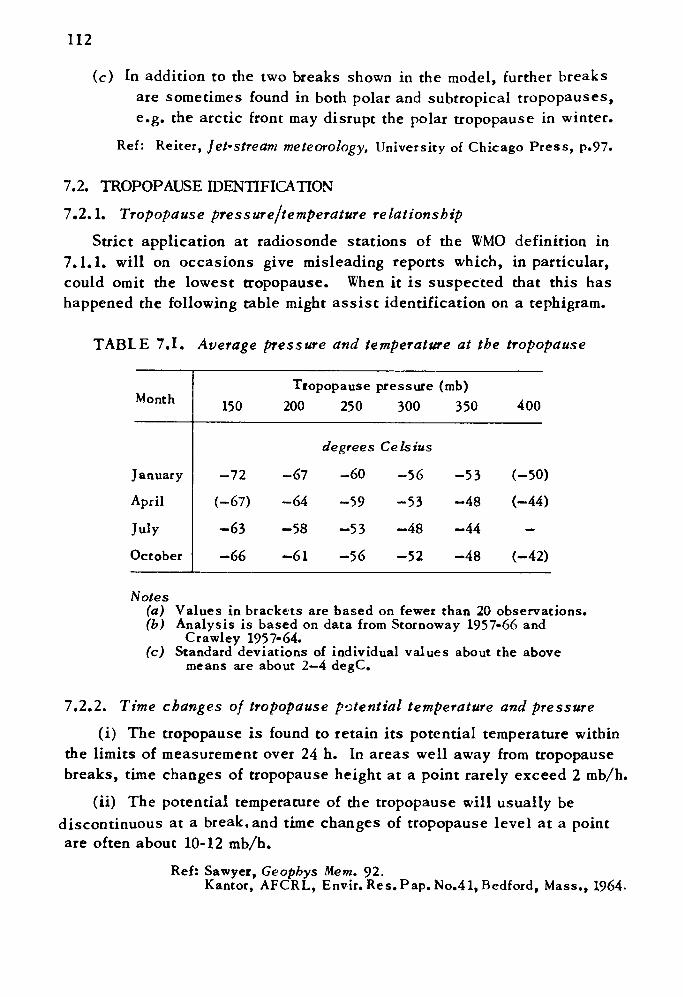
112
(c) In addition to the two breaks shown in the model, further breaks are sometimes found in both polar and subtropical tropopauses, e.g. the arctic front may disrupt the polar tropopause in winter.
Ref: Reiter, Jet'Stream meteorology. University of Chicago Press, p.97.
7.2. TROPOPAUSE IDENTIFICATION7.2.1. Tropopause pressure/temperature relationship
Strict application at radiosonde stations of the WMO definition in 7.1.1. will on occasions give misleading reports which, in particular, could omit the lowest tropopause. When it is suspected that this has happened the following table might assist identification on a tephigram.
TABLE 7.1. Average pressure and temperature at the tropopause
Month
January
April
July
October
150
-72
(-67)-63
-66
Tropopause 200 250
-67
-64
-58
-61
degrees
-60
-59
-53
-56
pressure 300
Celsius
-56
-53
-48
-52
(mb) 350
-53
-48
-44
-48
400
(-50)
(-44)—
(-42)
Notes(a) Values in brackets are based on fewer than 20 observations.(b) Analysis is based on data from Stornoway 1957-66 and
Crawley 1957-64.(c) Standard deviations of individual values about the above
means are about 2—4 degC.
7.2.2. Time changes of tropopause potential temperature and pressure(i) The tropopause is found to retain its potential temperature within
the limits of measurement over 24 h. In areas well away from tropopause breaks, time changes of tropopause height at a point rarely exceed 2 mb/h.
(ii) The potential temperature of the tropopause will usually be discontinuous at a break,and time changes of tropopause level at a point are often about 10-12 mb/h.
Ref: Sawyer, Geophys Mem. 92.Kantor, AFCRL, Envir. Res. Pap. No.41, Bedford, Mass., 1964-
113
7.3. SYNOPTIC AIDS TO THE CONSTRUCTION OF TROPOPAl'SF CHARTS
(i) Tropopause funnels (lows) are often of relatively small horizon tal dimensions, and their presence is therefore not necessarily indicated directly by the observations on a particular chart. Continuity usually gives a good guide to the position of all tropopause centres.
(ii) An independent check on the positions of tropopause centres may be obtained from the computed thermal winds at stations surrounding the centres. Tropopause funnels extending below the 300-mb level are normally aligned vertically with warm centres in the 300-200 mb thickness pattern, and tropopause domes (highs) extending above the 300-tnb level are aligned with warm pools in the 500-300 mb thickness pattern. Lines drawn through the positions of the radiosonde stations perpendicular to the thermal winds for the appropriate layer will therefore intersect near the position of the tropopause centre.
(iii) Tropopause funnel development (due to the descent and adiabatic warming of stratospheric air) will accompany strong divergence at the maxi mum wind level; this in its turn is normally associated with vigorous deepening of surface depressions.
(iv) Tropopause isopleth gradients are uneven, and show bands of strong gradient along tropopause breaks; thus, typically there will be two such bands on all hemispherical charts, but on occasions the two bands can merge into one. The best positional guide for these bands of strong gradient will therefore be the jet-core positions as determined on a maxi mum wind chart (or as roughly indicated by a 300-mb chart).
(v) If the thickness field indicates that little vertical motion is taking place near a front at high level, the advective component of motion will be dominant, and tropopause isopleths will move as if tied to the front.
Ref: Ogden (unpublished).
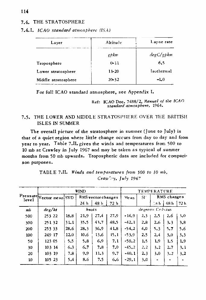
114
7.4. THE STRATOSPHERE7.4.1. 1CAO standard atmosphere (ISA)
Layer
Troposphere
Lower stratosphere
Middle stratosphere
Altitude
Zpkm0-11
11-20
20-32
Lapse rate
degC/gpkm
6.5
Isothermal
-1.0
For full ICAO standard atmosphere, see Appendix I.
Ref: ICAO Doc. 7488/2, Manual of the ICAO standard atmosphere, 1964.
7.5. THE LOWER AND MIDDLE STRATOSPHERE OVER THE BRITISH ISLES IN SUMMER
The overall picture of the stratosphere in summer (June to July) is that of a quiet region where little change occurs from day to day and from year to year. Table 7.II. gives the winds and temperatures from 500 to 10 mb at Crawley in July 1967 and may be taken as typical of summer months from 50 mb upwards. Tropospheric data are included for compari son purposes.
TABLE 7.II. Winds and temperatures from 500 to 10 mb,Craw'^y, July 1967
Pressure level
mb50030020010050302010
WINDVector mean
deg/kt253 22251 32253 33249 17123 05103 14103 19105 23
SVD RMSve 24 h
•ctorch 48 h
anges72 h
knots18.831.128.612.05.56.37.85.4
21.935.528.310.65.86.79.98.6
27.443.736.913.66.97.8
11.37.5
27.948.541.815.17.17.09.76.6
TEMPERATUREVie an sr RM
::4h5 chan48h
ges72 h
degrees (]e> !•=, ius-14.9-42.1-54.2-53.9-50.2-45.2-40.1-29.1
2.32.84.02.51.52.22.33.0
2.52.65.32.41.93.23.0-
2.63.35.73.01.52.73.2
-
3.0
3.85.63.31.93.13.2
-
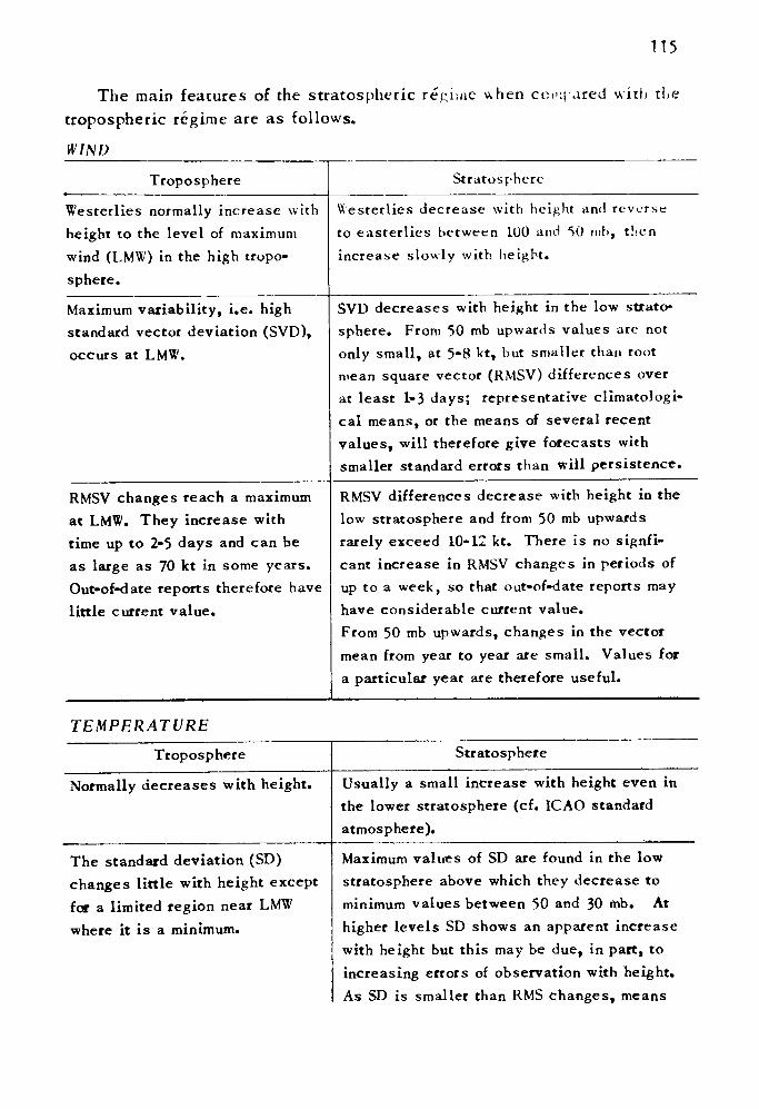
115
The main features of the stratospheric reissue when compared with the tropospheric regime are as follows.
WIND
Troposphere Stratosphere
Westerlies normally increase with height to the level of maximum wind (LMW) in the high tropo sphere.
Westerlies decrease with height and reverse
to easterlies between 100 and 50 nib, then increase slowly with height.
Maximum variability, i.e. high standard vector deviation (SVD), occurs at LMW.
SVD decreases with height in the low strato sphere. From 50 mb upwards values are not only small, at 5-8 kt, but smaller than root mean square vector (RMSV) differences over at least 1-3 days; representative climatologi-
cal means, or the means of several recent values, will therefore give forecasts with smaller standard errors than will persistence.
RMSV changes reach a maximum at LMW. They increase with time up to 2-5 days and can be as large as 70 kt in some years. Out-of-date reports therefore have little current value.
RMSV differences decrease with height in the low stratosphere and from 50 mb upwards rarely exceed 10-12 kt. There is no signfi- cant increase in RMSV changes in periods of up to a week, so that out-of-date reports may have considerable current value. From 50 mb upwards, changes in the vector
mean from year to year are small. Values for a particular year are therefore useful.
TEMPERATURE
Troposphere Stratosphere
Normally decreases with height. Usually a small increase with height even in the lower stratosphere (cf. ICAO standard atmosphere).
The standard deviation (SD) changes little with height except
for a limited region near LMW
where it is a minimum.
Maximum values of SD are found in the low stratosphere above which they decrease to minimum values between 50 and 30 mb. At
higher levels SD shows an apparent increase
with height but this may be due, in part, to
increasing errors of observation with height.
As SD is smaller than RMS changes, means
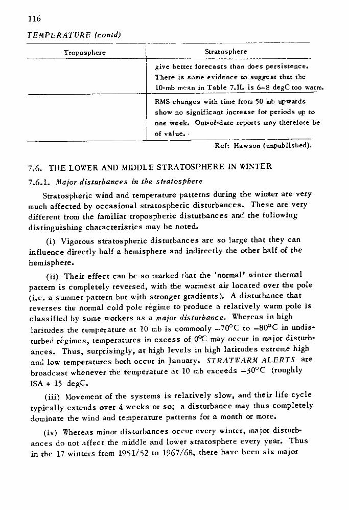
116
TEMPERATURE (contd)
Troposphere Stratosphere
give better forecasts than does persistence. There is some evidence to suggest that the 10-mb mean in Table 7.II. is 6—8 degC too warm.
RMS changes with time from 50 mb upwards show no significant increase for periods up to one week. Out-of-date reports may therefore be of value. •
Ref: Hawson (unpublished).
7.6. THE LOWER AND MIDDLE STRATOSPHERE IN WINTER
7.6.1. Major disturbances in the stratosphere
Stratospheric wind and temperature patterns during the winter are very much affected by occasional stratospheric disturbances. These are very different trom the familiar tropospheric disturbances and the following distinguishing characteristics may be noted.
(i) Vigorous stratospheric disturbances are so large that they can influence directly half a hemisphere and indirectly the other half of the hemisphere.
(ii) Their effect can be so marked that the 'normal* winter thermal pattern is completely reversed, with the warmest air located over the pole (i.e. a summer pattern but with stronger gradients). A disturbance that reverses the normal cold pole regime to produce a relatively warm pole is classified by some workers as a major disturbance. Whereas in high latitudes the temperature at 10 mb is commonly — 70°C to —80°C in undis turbed regimes, temperatures in excess of 0°C may occur in major disturb ances. Thus, surprisingly, at high levels in high latitudes extreme high and low temperatures both occur in January. STRATWARM ALERTS are broadcast whenever the temperature at 10 mb exceeds -30°C (roughly ISA + 15 degC.
(iii) Movement of the systems is relatively slow, and their life cycle typically extends over 4 weeks or so; a disturbance may thus completely dominate the wind and temperature patterns for a month or more.
(iv) Whereas minor disturbances occur every winter, major disturb ances do not affect the middle and lower stratosphere every year. Thus in the 17 winters from 1951/52 to 1967/68, there have been six major
117
disturbances, starting in January of 1952, 1957, 1958, 1963 and December of 1965 and 1967. (There is some evidence that major disturbances occur more frequently in the upper stratosphere, from which level only a proport ion extend their influence downwards to the middle and lower stratosphere.)
(v) Variations of temperature following the flow can be quite spect acular, much more so than time variations at a point. The high temperatures in an area of stratospheric warming are largely caused dynamically by descent through the pressure surfaces, and the areas of warmest air corres pond to the lowest point of the trajectories. The centres of maximum temperature at each level are not aligned vertically; slopes of the axes joining warm centres at progressively higher levels of about 1:200 have been measured between 50 and 10 mb.
Ref: Hawson (unpublished).
7.6.2. Mean values of wind and temperature over the British Isles
As a result of the characteristics of stratospheric disturbances noted in 7.6.1. the frequency distributions are abnormal; values of both wind and temperature meaned over a number of winter seasons are therefore of little help to the analyst. Similarly, mean values for a particular winter may give little guidance about the values in any one month. Better guidance to winter stratospheric conditions is given by values of means, SD, and RMS changes for particular months from single years.
The figures for January 1967 given in Table 7.III. may be taken as representative of the winter stratosphere during a year in which no major disturbance occurs. The values of wind and temperature to be expected during a stratospheric disturbance will clearly depend on its position relative to the British Isles. The figures for January 1968 (during which a major disturbance was centred near Greenland), Table 7.IV., are typical only of conditions on the SE flank of a disturbance, some way from the centre; they do, however, indicate the possible departures from conditions in an undisturbed regime. In the development stage of a disturbance, Wly winds of 150 kt have been recorded at 50 mb on the northern flank of the warm thermal centre, compared with the undisturbed normal of about 40 kt.
7.6.3. Data for an undisturbed winter, January 1967 at CraivleyTable 7.IH. may be taken as typical of an undisturbed winter regime.
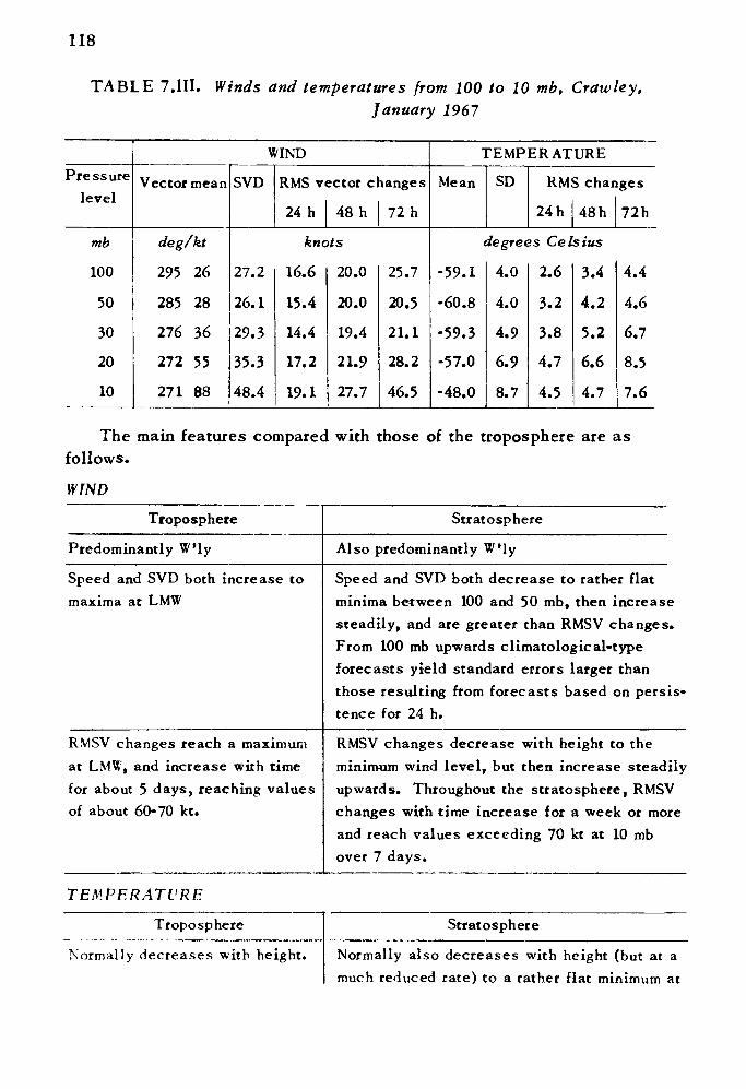
118
TABLE 7.III. Winds and temperatures from 100 to 10 mb, Crawley,January 1967
Pressure level
mb
100
50
30
20
10
WIND
Vector mean
deg/kt
295 26
285 28
276 36
272 55
271 88
SVD RMS v
24 h
ector c
48 h
banges
72 h
knots
27.2
26.1
29.3
35.3
48.4
16.6
15.4
14.4
17.2
19.1
20.0
20.0
19.4
21.9
27.7
25.7
20.5
21.1
28.2
46.5
TEMPERATURE
Mean SD RM
24 h
§ char
48 h
ges
72h
degrees Celsius
-59.1
-60.8
-59.3
-57.0
-48.0
4.0
4.0
4.9
6.9
8.7
2.6
3.2
3.8
4.7
4.5
3.4
4.2
5.2
6.6
4.7
4.4
4.6
6.7
8.5
7.6
The main features compared with those of the troposphere are as follows.
WIND
Troposphere
Predominantly W'ly
Stratosphere
Also predominantly W'ly
Speed and SVD both increase to maxima at LMW
Speed and SVD both decrease to rather flat minima between 100 and 50 mb, then increase steadily, and are greater than RMSV changes. From 100 mb upwards climatological-type forecasts yield standard errors larger than those resulting from forecasts based on persis tence for 24 h.
RMSV changes reach a maximum at LMW, and increase with time for about 5 days, reaching values of about 60-70 kt.
RMSV changes decrease with height to the minimum wind level, but then increase steadily upwards. Throughout the stratosphere, RMSV changes with time increase for a week or more and reach values exceeding 70 kt at 10 mb over 7 days.
TEMPERATURE
Troposphere
Normally decreases with height.
Stratosphere
Normally also decreases with height (but at much reduced rate) to a rather flat minimum
a at
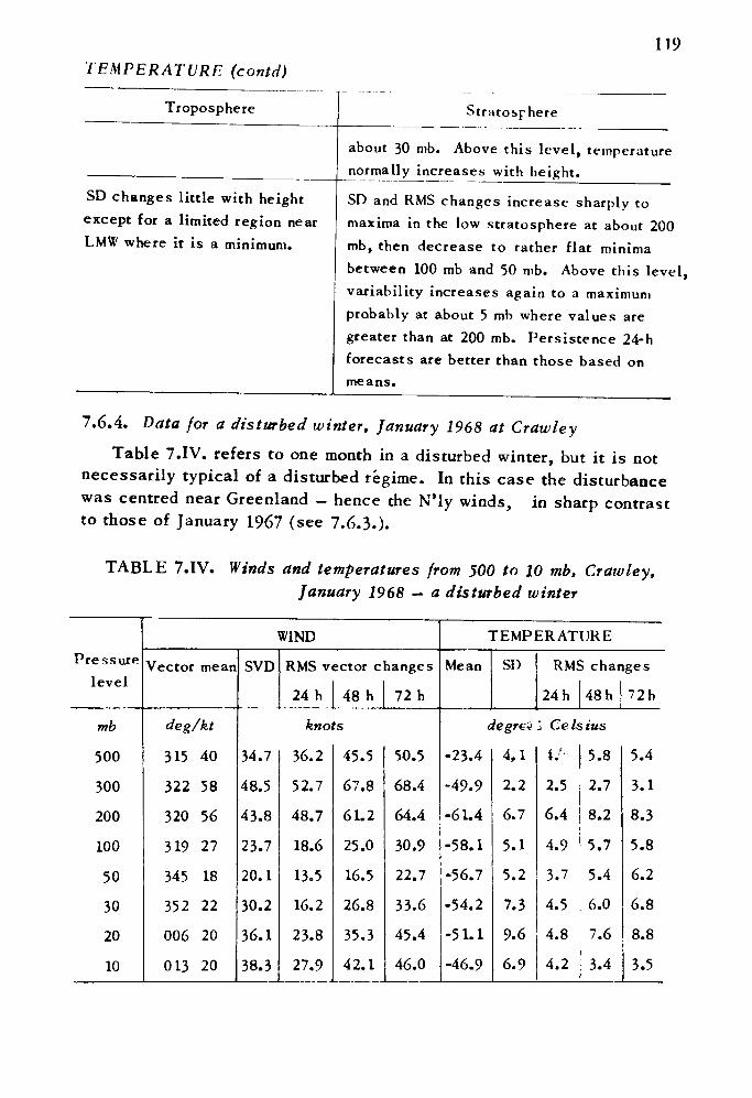
119TEMPERATURE (contd)
Troposphere
SD changes little with height except for a limited region near LMW where it is a minimum.
Stratosphere
about 30 mb. Above this level, temperature normally increases with height.
SD and RMS changes increase sharply to maxima in the low stratosphere at about 200 mb, then decrease to rather flat minima between 100 mb and 50 mb. Above this level, variability increases again to a maximum probably at about 5 mb where values are greater than at 200 mb. Persistence 24-h forecasts are better than those based on means.
7.6.4. Data lor a disturbed winter, January 1968 at CrawleyTable 7.IV. refers to one month in a disturbed winter, but it is not
necessarily typical of a disturbed regime. In this case the disturbance was centred near Greenland — hence the N'ly winds, in sharp contrast to those of January 1967 (see 7.6.3.).
TABLE 7.IV. Winds and temperatures from 500 to 10 mb. Crawley,January 1968 — a disturbed winter
Pressure level
mb
500
300
200
100
50
30
20
10
WIND
Vector mean
deg/kt
315 40
322 58
320 56
319 27
345 18
352 22
006 20
013 20
SVD RMS v<24 h
jctor cl
48 h
langes
72 h
knots
34.7
48.5
43.8
23.7
20.1
30.2
36.1
38.3
36.2
52.7
48.7
18.6
13.5
16.2
23.8
27.9
45.5
67.8
61.2
25.0
16.5
26.8
35.342.1
50.5
68.4
64.4
30.9
22.7
33.6
45.4
46.0
TEMPERATURE
Mean SO RMS
24 h
chan
48 h
ges
72h
degrei 1 Cels ius
-23.4
-49.9
-61.4
-58.1
-56.7
-54.2-51.1
-46.9
4,1
2.2
6.7
5.1
5.2
7.3
9.6
6.9
*/- | 5.8
2.56.4
4.9
3.7
2.7
8.2
5.7
5.4
4.5
4.8
6.0
7.6|
4.2 j 3.4
5.4
3.1
8.3
5.8
6.2
6.8
8.8
3.5
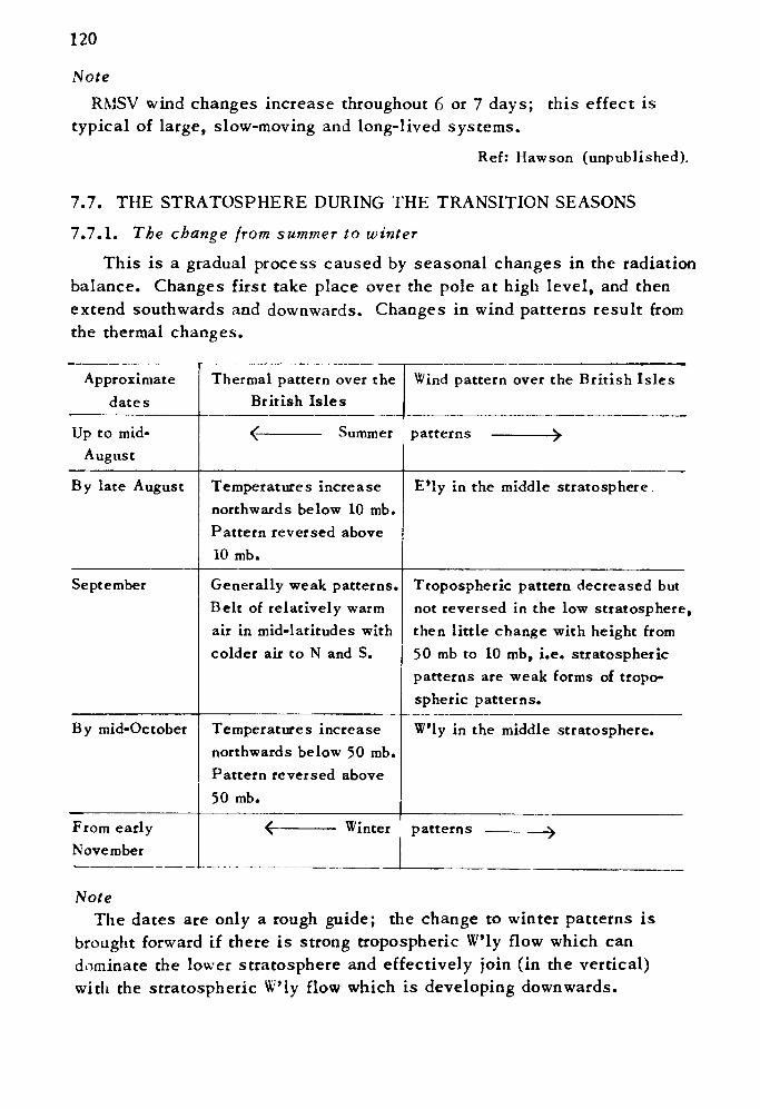
120
NoteRMSV wind changes increase throughout 6 or 7 days; this effect is
typical of large, slow-moving and long-lived systems.
Ref: Hawson (unpublished).
7.7. THE STRATOSPHERE DURING THE TRANSITION SEASONS
7.7.1. The change from summer to winter
This is a gradual process caused by seasonal changes in the radiation balance. Changes first take place over the pole at high level, and then extend southwards and downwards. Changes in wind patterns result from the thermal changes.
Approximate dates
Up to mid- August
Thermal pattern over the British Isles
Wind pattern over the British Isles
Summer patterns
By late August Temperatures increase northwards below 10 mb. Pattern reversed above 10 mb.
E'ly in the middle stratosphere.
September Generally weak patterns, Belt of relatively warm air in mid-latitudes with colder air to N and S.
Tropospheric pattern decreased but not reversed in the low stratosphere, then little change with height from 50 mb to 10 mb, i.e. stratospheric patterns are weak forms of tropo- spheric patterns.
By mid-October Temperatures increase northwards below 50 mb. Pattern reversed above 50 mb.
Wly in the middle stratosphere.
Winter patternsFrom early November
NoteThe dates are only a rough guide; the change to winter patterns is
brought forward if there is strong tropospheric Wly flow which can dominate the lower stratosphere and effectively join (in the vertical) with the stratospheric Wly flow which is developing downwards.
121
7.7.2. The change from winter to summer
Over the British Isles persistent E'ly wind components at 50 mb have first been observed as early as mid-March and as late as late May, whilst in 4 years out of 12 (1957-68) the first appearance occurred during the second half of May. In any one year the first appearance of the E'ly wind components was earlier the higher the level considered.
After a major disturbance which causes a warm pole to develop dynamically, the situation will generally revert to the normal cold-pole regime; in such years there is a tendency for the transition to be late. But if the disturbance forms in late winter (say, late January onwards) its life cycle will last through February into March. If the warm pole is still present giving stratospheric easterlies in mid-March, the cold pole will not re-forua and the summer pattern is effectively established already.
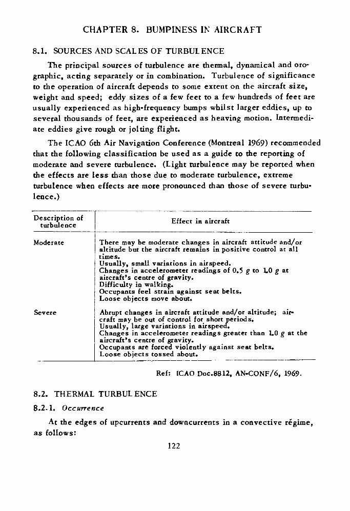
CHAPTER 8. DUMPINESS IN AIRCRAFT
8.1. SOURCES AND SCALES OF TURBULENCEThe principal sources of turbulence are thermal, dynamical and oro-
graphic, acting separately or in combination. Turbulence of significance to the operation of aircraft depends to some extent on the aircraft size, weight and speed; eddy sizes of a few feet to a few hundreds of feet are usually experienced as high-frequency bumps whilst larger eddies, up to several thousands of feet, are experienced as heaving motion. Intermedi ate eddies give rough or jolting flight.
The ICAO 6th Air Navigation Conference (Montreal 1969) recommended that the following classification be used as a guide to the reporting of moderate and severe turbulence. (Light turbulence may be reported when the effects are less than those due to moderate turbulence, extreme turbulence when effects are more pronounced than those of severe turbu lence.)
Description of turbulence Effect in aircraft
Moderate
Severe
There may be moderate changes in aircraft attitude and/oraltitude but the aircraft remains in positive control at alltimes.Usually, small variations in airspeed.Changes in accelerometer readings of 0.5 g to 1.0 g ataircraft's centre of gravity.Difficulty in walking.Occupants feel strain against seat belts.Loose objects move about.
Abrupt changes in aircraft attitude and/or altitude; air craft may be out of control for short periods. Usually, large variations in airspeed.Changes in accelerometer readings greater than LO g at the aircraft's centre of gravity.Occupants are forced violently against seat belts. Loose objects tossed about.
Ref: ICAO Doc.8812, AN-CONF/6, 1969.
8.2. THERMAL TURBULENCE 8.2-1. Occurrence
At the edges of upcurrents and downcurrents in a convective regime, as follows:
122
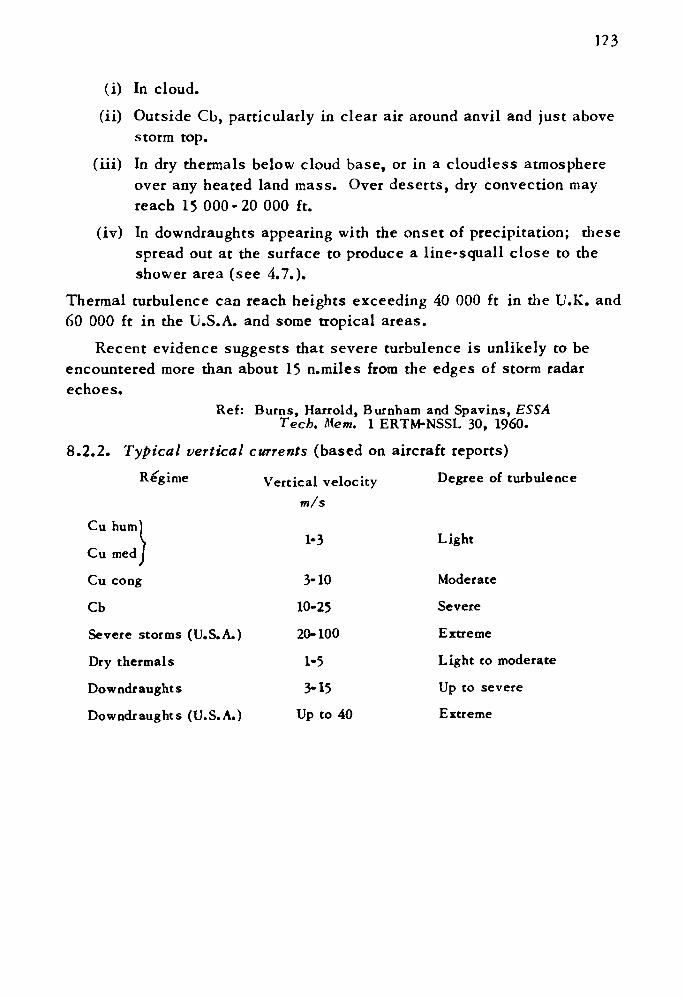
(i) In cloud.
(ii) Outside Cb, particularly in clear air around anvil and just above storm top.
(iii) In dry thermals below cloud base, or in a cloudless atmosphere over any heated land mass. Over deserts, dry convection may reach 15 000-20 000 ft.
(iv) In downdraughts appearing with the onset of precipitation; these spread out at the surface to produce a line-squall close to the shower area (see 4.7.).
Thermal turbulence can reach heights exceeding 40 000 ft in the U.K. and 60 000 ft in the U.S.A. and some tropical areas.
Recent evidence suggests that severe turbulence is unlikely to be encountered more than about 15 n.miles from the edges of storm radar echoes.
Ref: Burns, Harrold, Burnham and Spavins, ESS A Tech. Mem. 1 ERTM-NSSL 30, I960.
8.2.2. Typical vertical currents (based on aircraft reports)
Regime Vertical velocity Degree of turbulence
m/s
Cu hum)\ 1-3 Light
Cu medl
Cu cong 3-10 Moderate
Cb 10-25 Severe
Severe storms (U.S.A.) 20-100 Extreme
Dry thermals 1-5 Light to moderate
Downdraughts 3-15 Up to severe
Downdraughts (U.S.A.) Up to 40 Extreme
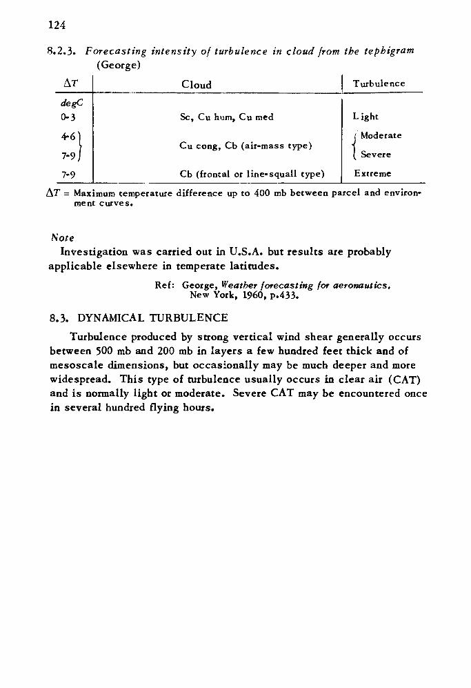
124
8.2.3. Forecasting intensity of turbulence in cloud from the tephigram (George)
AT Cloud Turbulence
Sc, Cu hum, Cu med
Cu cong, Cb (air-mass type)
Cb (frontal or line-squall type)
Light
I Moderate
( Severe
Extreme
AT = Maximum temperature difference up to 400 mb between parcel and environ ment curves.
NoteInvestigation was carried out in U.S.A. but results are probably
applicable elsewhere in temperate latitudes.Ref: George, Weather forecasting for aeronautics,
New York, I960, p.433.
8.3. DYNAMICAL TURBULENCETurbulence produced by strong vertical wind shear generally occurs
between 500 mb and 200 mb in layers a few hundred feet thick and of mesoscale dimensions, but occasionally may be much deeper and more widespread. This type of turbulence usually occurs in clear air (CAT) and is normally light or moderate. Severe CAT may be encountered once in several hundred flying hours.
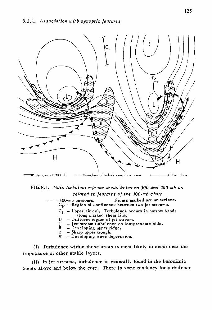
8.3.1. Association with synoptic features
125
Jet axis at 300mb •"" ~— Boundary of turbulence -prone areas
H
-i Shear line
FIG.8.1. Main turbulence-prone areas between 500 and 200 mb as related to features of the 300-mb chart
——— 300-mb contours. Fronts marked are at surface. Cp — Region of confluence between two jet streams.CT — Upper air col. Turbulence occurs in narrow bands
along marked shear line. D — Diffluent region of jet stream. J — Jet-stream turbulence on low-pressure side. R — Developing upper ridge. T — Sharp upper trough. W — Developing wave depression.
(i) Turbulence within these areas is most likely to occur near the tropopause or other stable layers.
(ii) In jet streams, turbulence is generally found in the baroclinic zones above and below the core. There is some tendency for turbulence
126
to be concentrated in the lower zone of cyclonically curved jets and in the upper zone of anticyclonically curved jets.
Ref: HWF 20.2.5.
(iii) There is some qualitative evidence that turbulence is more likely to be severe within turbulence-prone areas if rapid change or development in the upper air pattern is occurring locally than if the pattern is relatively static.
Ref: Roach, Met.Mag., Mar. '69. Lennie, Met.Mag., Jan. '69'
8.3.2. Effect of topographyThe incidence of CAT is more frequent over land, particularly over
mountains, than over the sea. It is not possible to give precise quantita tive values to this difference but it is suggested that a factor of 3 or more over most land areas, increasing perhaps to 10 over very mountain ous are as, is reasonable.
Ref: Turner, Met.Mag.. Feb. '59.Clodman and Ball, New York Univ., Coll. Eng.
Res. Div., AFCRL Contract No. AF 19(604)-3068, 1959.
Col son, WMO Tech. Note 95, 1969.
8.4. OROGRAPHIC TURBULENCE
8.4.1. Low-level turbulenceThe following table gives a rough guide to the subjective intensities
of turbulence to be expected in the lowest few hundred feet.
Surface wind
knots 15-35
>35
Turbulence over:
Sea Flat country
Light— moderate Moderate
Moderate— severe Severe
Hill country
Severe
Extreme
NoteStrong sunshine added to strong wind may increase handling diffi
culties with aircraft on landing and take-off.
Ref: Zbrozek, RAE Tech. Note AERO 2681, I960. Pasquill (unpublished).
8.4.2. Squalls near the surfaceViolent squalls create the most dangerous low-level hazard to aircraft,
and may arise as follows:
(i) During or preceding the passage of an active cold front.
127
(ii) During or preceding the passage of a thunderstorm, (see 4.7.)
(iii) In hilly or mountainous country in association with 'rotor streaming', which requires:
(a) Strong winds at low levels (20-30 kt or more).
(b) Winds decreasing sharply or even reversing direction at 1% to 2 times the height of the hills.
(c) A stable air mass (apart from stirring in the lowest layers).
Ref: Met. Rep. No. 18.
8.4.3. Mountain waves
Mountain waves and associated turbulence may be pronounced when the following conditions are all satisfied:
(i) A wind blowing within 30° of normal to a substantial range of hills.
(ii) A wind speed of 20 kt or more at hill-crest level, with speed increasing with height but with little change of direction (strong waves are often associated with jet streams).
(iii) A stable layer somewhere between hill-crest level and a few thousand feet above.
Notes
(a) Turbulence-prone areas are generally near wave crests and troughs.
(b) These rules may be applied in a quantitative manner by using Scorer's parameter, /2.
Ref: Met. Rep. No. 18, App. I.Casswell, Met.Mctg., Mar. '66.
8.4.4. Rotor-zone turbulence
A rotor zone (not the same phenomenon as 'rotor streaming* of 8.4.2.(iii)) is a region of violent turbulence sometimes found somewhat above and to the lee of a large mountain ridge; its formation requires a well-defined lee escarpment and strongly developed lee waves. The rotor may, or may not, be indicated by a long roll of ragged cumulus or stratocumulus parallel to the main ridge. Rotor clouds are rare in the U.K. but die 'Helm Bar* of Crossfell is one example.
Ref: Met. Rep. No. 18.
CHAPTER 9. ICE ACCRETION ON AIRCRAFT
9.1. TYPES OF ICING
Type
Hoar frost
Rime
Rain ice
Pack snow
Source
Vapour
Supercooleddrops
Supercooledrain
Supercooleddrops andsnowf lakes
Formation and properties
Direct deposition on surface with temperaturebelow frost-point of ambient air. White, crystal
line coating.
Impact on surface below 0°C. Variable properties;
two extreme forms described below:(a) Opaque rime: drops freeze without muchspreading; light porous texture with large
amount of entrapped air.(b) Clear or glaze ice: drops spread beforefreezing; smooth, glassy; sticks strongly to
surfaces.
Formation as clear ice. Substantial deposit mayform over extensive area. Rare.
Drops freeze on impact, embedding snowflakes.
Ref: HWF 18.2.
9.2. GENERAL REMARKSIcing is very variable in both space and time in any cloud system, and
any forecast must necessarily be of probabilities. The following remarks are therefore of a statistical nature.
(i) Since the number of water droplets intercepted depends upon the shape and speed of the aircraft, so will the icing. However, it is use ful to generalize by regarding supercooled liquid water contents of clouds of 0.5 and 1.0 g/m 3 as separating 'light', 'moderate' and 'severe* icing.(ii) Rain or cloud encountered by a cold aircraft descending may produce icing until the aircraft has warmed up. Intensity may be severe, particularly on forward-facing transparencies.
128
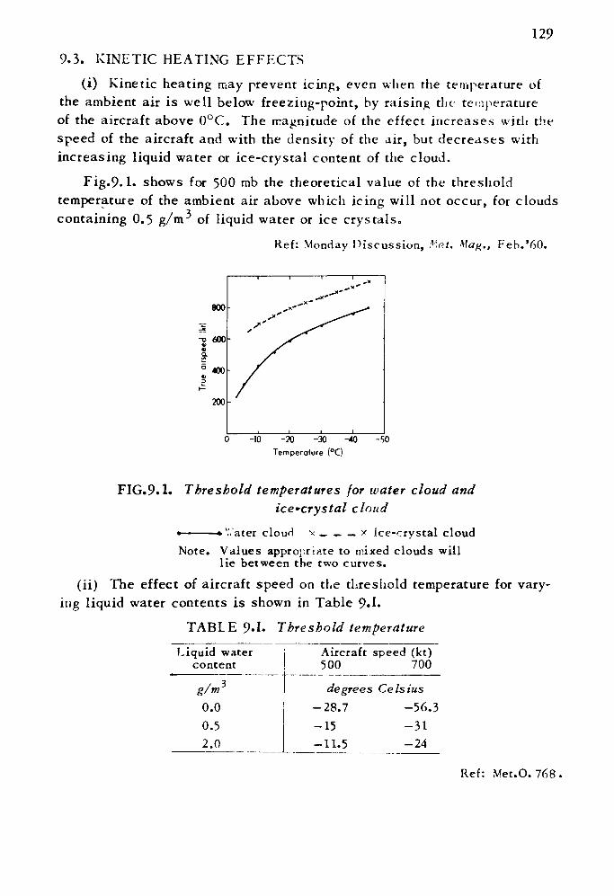
129
9.3. KINETIC HEATING EFFECTS
(i) Kinetic heating may prevent icing, even when the temperature of the ambient air is well below freezing-point, by raising the temperature of the aircraft above 0°C. The magnitude of the effect increases with the speed of the aircraft and with the density of the air, but decreases with increasing liquid water or ice-crystal content of the cloud.
Fig.9.1. shows for 500 mb the theoretical value of the threshold temperature of the ambient air above which icing will not occur, for clouds containing 0.5 g/m of liquid water or ice crystals.
Ref: Monday Discussion, Kvt. /Vfa#.. Feb.'60.
800
I
200
-10 -20 -30Temperature (°C)
-50
FIG.9.1. Threshold temperatures for water cloud andice'crystal cloud
»————»'.Vater cloud v_ _ _ x ice-crystal cloudNote. Values appropriate to mixed clouds will
lie between the two curves.
(ii) The effect of aircraft speed on the threshold temperature for vary ing liquid water contents is shown in Table 9.1.
TABLE 9«I. Threshold temperature
Liquid water content
0.0 0.5 2.0
Aircraft speed (kt) 500 700
degrees Celsius-28.7 -56.3-15 -31-11.5 -24
Ref: Met.O. 768,
130
9.4. VARIATION WITH CLOUD TYPE
Type of cloud
Cu Cb NsSc Ac
Ac with AsAs
St
Probability of icing
High= 50%
Low
Low
Intensity
May be severeRarely more
than moderateModerate or
lightLight
Water content
g/m0.2-4.00. 1-0.5
0.1-0.3
0.1-0.5
Note
Ref: HWF 18.4.2.Mason, B.J., Physics of clouds, 1957.
In supercooled Sc relatively large liquid water contents may persist over many tens of miles near the upper boundary of the cloud layer. Moderate or severe icing can occur in these circumstances if an aircraft remains at this particular height.
9.5. CLOUD PROPERTIES AND ICING RISK
9.5.1. Connective clouds (Cu and Cb)At temperatures of —40°C or below water droplets are very rare and
the probability of icing is very low.Between —40 and —20^ ice crystals greatly predominate and slight
icing is likely, but moderate icing may occur for short periods in new, vigorously developing cloud cells.
Between —20 and 0°C there are few ice crystals and icing may be severe over a substantial depth of cloud and for a wide range of cloud- base temperatures. Use Fig.9.2. to determine intensity of icing in these cases.
Ref: HWF 18.4., 18.5. Met.O.768.
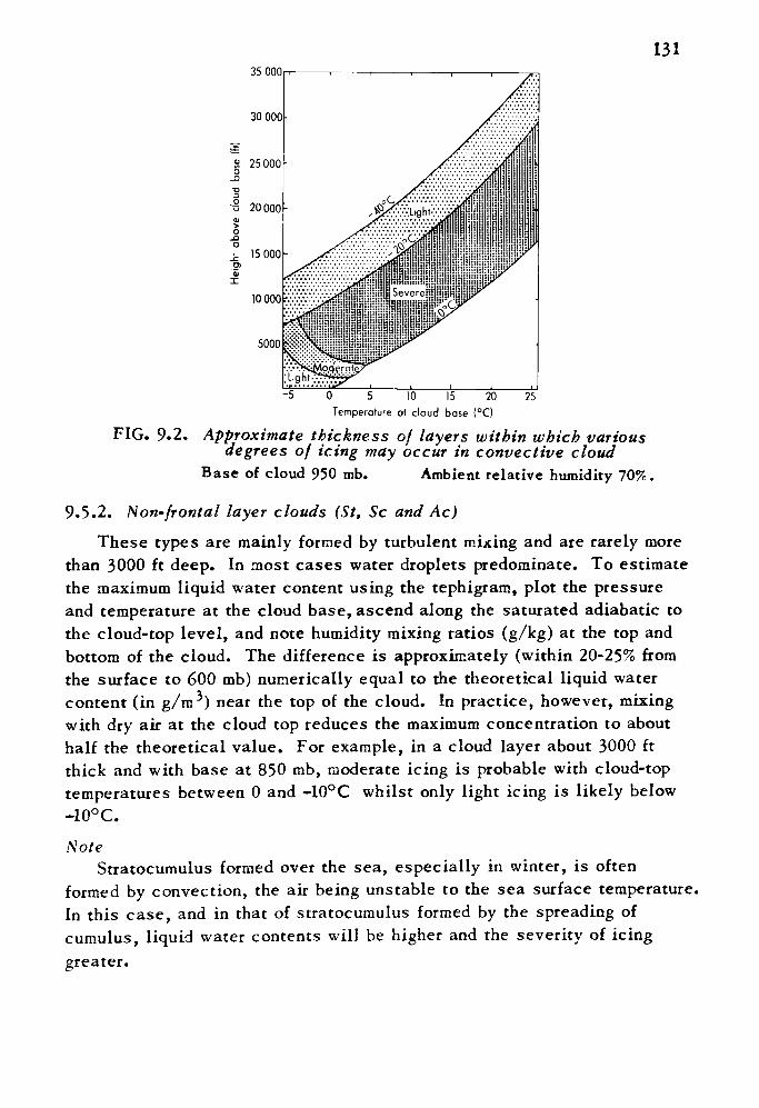
13135 OOOrr
~0"~ ~T ~KT 15 20 Temperature at cloud base (°C)
FIG. 9.2. Approximate thickness of layers within which various degrees of icing may occur in convective cloud
Base of cloud 950 mb. Ambient relative humidity 70% .
9.5.2. Non-frontal layer clouds (St, Sc and Ac)These types are mainly formed by turbulent mixing and are rarely more
than 3000 ft deep. In most cases water droplets predominate. To estimate the maximum liquid water content using the tephigram, plot the pressure and temperature at the cloud base, ascend along the saturated adiabatic to the cloud-top level, and note humidity mixing ratios (g/kg) at the top and bottom of the cloud. The difference is approximately (within 20-25% from the surface to 600 mb) numerically equal to the theoretical liquid water content (in g/m 3 ) near the top of the cloud. In practice, however, mixing with dry air at the cloud top reduces the maximum concentration to about half the theoretical value. For example, in a cloud layer about 3000 ft thick and with base at 850 mb, moderate icing is probable with cloud-top temperatures between 0 and -10°C whilst only light icing is likely below
NoteStratocumulus formed over the sea, especially in winter, is often
formed by convection, the air being unstable to the sea surface temperature. In this case, and in that of Stratocumulus formed by the spreading of cumulus, liquid water contents will be higher and the severity of icing greater.
132
9.5.3. Frontal layer clouds
These are formed by the slow ascent of a large mass of air and may be many thousands of feet deep. When associated with widespread con tinuous light precipitation they are mainly composed of ice crystals and snowflakes . Light icing is probable but is confined to a shallow layer (usually about 1000 ft deep) immediately above the 0°C surface.
The chance of severe icing is much increased with the more active fronts, especially where orographic uplift is present.
9.5.4. Ice-crystal clouds
These are not normally considered an icing hazard. However, a few cases of airframe icing have been reported, possibly arising from kinetic heating near the 'stagnation* points (the leading edges of structures where a small element of the flow is reduced to rest) of high-speed air craft. This possibility must be increasingly borne in mind as aircraft speeds rise.
As the water content of cirriform clouds is quite small, icing will be only light but may still constitute a hazard as the cloud is often difficult to detect from an aircraft and because quite small amounts of icing of intakes, struts and guide vanes can cause compressor stall and flame- out of axial-flow jet engines.
A similar effect can occur when there is an accumulation of ice crystals or snowflakes in a jet engine intake, but this is a hazard only when the concentration of ice crystals is particularly high as in vigorous . Cb in the tropics.
9.5.5. Orographic cloud
In cloudy lir forced to rise over high ground the liquid water content is higher than in similar air elsewhere.
Air which is stable elsewhere may become unstable over and near high ground ('potential instability'). Thus a weak front may become active over high ground and deep layer cloud may contain vigorous convective cells in which the water content is very high because of the protective cloudy environment. Severity of icing is increased in these cases.
A further effect which should be watched for when a stable layer is lifted bodily is the lowering of the 0°C level which may occur as a result of adiabatic cooling.
Ref: HWF 18,4., 18.5.
13?
9.6. ICING ASSOCIATED WITH FRONTS A\T) PRFr IPITATION
Icing associated with fronts and depressions is very variable and each case should be treated on its merits. However, the following rules give some general guidance.
9.6.1. T'/r*v fronts
In active warm fronts the possibility of severe icing should be indica ted within 100 miles of the surface front; if the front is particularly active, the distance should be increased to 200 miles.
Notes
(a) If upper-level instability can be inferred the probability of severe icing should be increased.
(b) Severe rime icing may be encountered in As/Ns as much as 300 miles ahead of the surface front.
(c) Freezing rain (rain ice) ahead of a warm front can produce severe icing, but occurs only rarely.
9.6.2. Cold fronts
Severe icing may occur within 50-100 miles of the surface front, especially if it is active and there is a copious supply of moisture ahead.
9.6.3. Depressions with ill-defined fronts
In the thick cloud associated with the centre of a depression where the fronts are ill defined, severe icing may occur within 250 miles of the centre, particularly in the northern and western sectors.
Ref: HWF 18.5.3., 18.5.4. Jones, MRP 1017.
9.7. ENGINE ICING
(i) Older types of piston engine are prone to carburettor icing because of adiabatic cooling of the air in the venturi and evaporation of the fuel. Increasing use of fuel injection systems makes this rare.
(ii) Turbine and pure jet engines are affected by icing of the intake rim, struts across the intake and guide vanes. Centrifugal engines are relatively insensitive but quite light icing can cause compressor stall in axial-flow engines (see 9.5.4. above).
(iii) Adiabatic expansion in the intake of jet engines at low forward speeds (e.g. on the approach or during take-off) may cause a drop in the temperature of intake air of around 5 degC. Engine icing may then occur at ambient temperatures around or above 0°C in a potentially hazardoussituation.
Ref:
134
9.8. HELICOPTER ICING
The effects of icing on helicopters are potentially more serious than on fixed-wing aircraft because:
(i) Wing (i.e. blade) loading is higher and aerodynamic effects therefore greater.(ii) Extra blade weight due to icing may increase centrifugal
forces on the rotor hub to unacceptable limits.(iii) Slight asymmetries in the amount of icing on individual blades may set up severe vibration of the rotor assembly.(iv) Icing may interfere with the operation of the cyclic-pitch control and hence control of the aircraft.
Note that since blade airspeed varies along the rotor blade, so does the severity of icing.
Ref: Met.O.768.
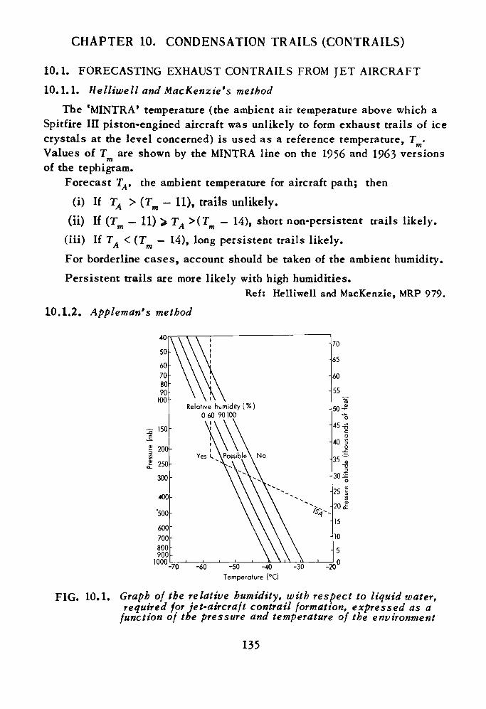
CHAPTER 10. CONDENSATION TRAILS (CONTRAILS)
10.1. FORECASTING EXHAUST CONTRAILS FROM JET AIRCRAFT
10.1.1. Helliwell and MacKenzie's method
The 'MINTRA* temperature (the ambient air temperature above which a Spitfire HI piston-engined aircraft was unlikely to form exhaust trails of ice crystals at the level concerned) is used as a reference temperature, T - Values of Tm are shown by the MINTRA line on the 1956 and 1963 versions of the tephigram.
Forecast TA , the ambient temperature for aircraft path; then
(i) If TA > (Tm - 11), trails unlikely.(ii) If (Tm - 11) > TA >(Tm - 14), short non-persistent trails likely.
(iii) If TA < (Tm - 14), long persistent trails likely.
For borderline cases, account should be taken of the ambient humidity.
Persistent trails are more likely with high humidities.Ref: Helliwell and MacKenzie, MRP 979.
10.1.2. Appleman's method
40
50
60708090
100
2 '50__§| 200
I 250
300
400 '500
600700800900
1000
Relative humidity (%) 060 90100
<a
-70 -60 -50 -40
Temperature (°C)-30 -20
70
65
60
55
50^ "o
45^C O
40 3 o-C
35 t"D
30 J o25 § •a20 1
15
10
50
I CIII|^CI UIUI C V >— I
FIG. 10.1. Graph of the relative humidity, with respect to liquid water, required for jet-aircraft contrail formation, expressed as a
function of the pressure and temperature of the environment
135
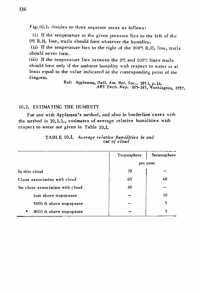
136
Fig. 10.1. divides to three separate areas as follows:
(i) If the temperature at the given pressure lies to the left of the 0% R.H. line, trails should form whatever the humidity, (ii) If the temperature lies to the right of the 100% R.H. line, trails
should never form.(iii) If the temperature lies between the 0% and 100^ lines trails should form only if the ambient humidity with respect to water is at least equal to the value indicated at the corresponding point of the diagram.
Ref: Appleman, Bull. Am. Met. Soc., 1953, p. 14.AWS Tech. Rep. 105-145, Washington, 1957.
10.2. ESTIMATING THE HUMIDITY
For use with Appleman's method, and also in borderline cases with the method in 10.1.1., estimates of average relative humidities with respect to water are given in Table 10.1.
TABLE 10.1. Average relative humidities in andout of cloud
In thin cloud
Close association with cloud
No close association with cloud
just above tropopause
5000 ft above tropopause
* 8000 ft above tropopause
Troposphere Stratosphere
per cent
70
60
40
40
10
5
5
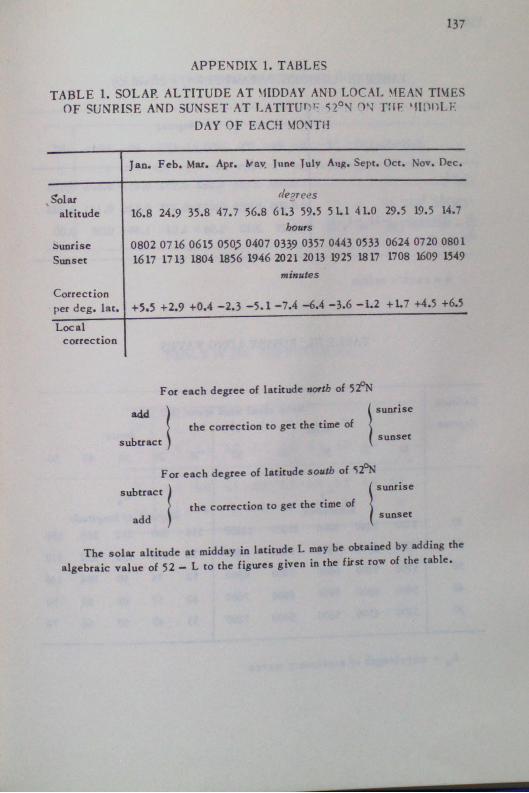
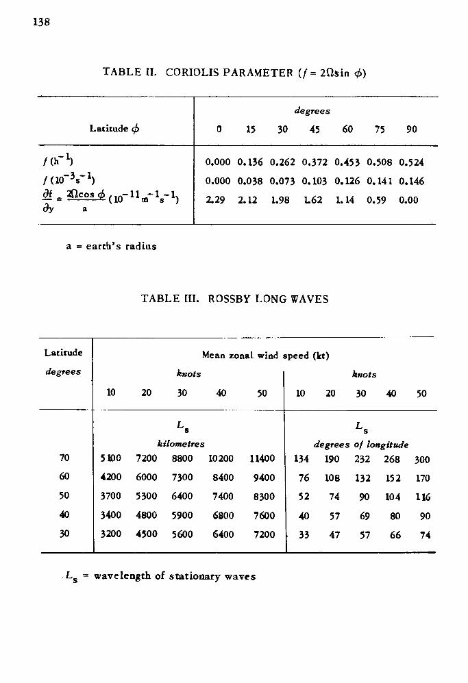
138
TABLE II. CORIOLIS PARAMETER (/» ZQsin
Latitude 0 15
degrees
30 45 60 75 90
/or 1)
dy a
0.000 0.136 0.262 0.372 0.453 0.508 0.524
0.000 0.038 0.073 0.103 0.126 0.141 0.1462.29 2.12 1.98 L62 1.14 0.59 0.00
a = earth's radius
TABLE III. ROSSBY LONG WAVES
Latitude
degrees
70
60
50
40
30
Mean zonal wind speed
10
5100
4200
3700
3400
3200
20
knots
30
L s
kilometres 7200 8800
6000
5300
4800
4500
7300
6400
5900
5600
40
10200
8400
7400
6800
6400
50
11400
9400
8300
7600
7200
10
134
7652
40
33
(kt)
20
degrees 190
108
74
5747
knots
30
Ls
40
of longitude 232 268
132
90
69
57
152
104
80
66
50
300
170
116
90
74
LS = wavelength of stationary waves
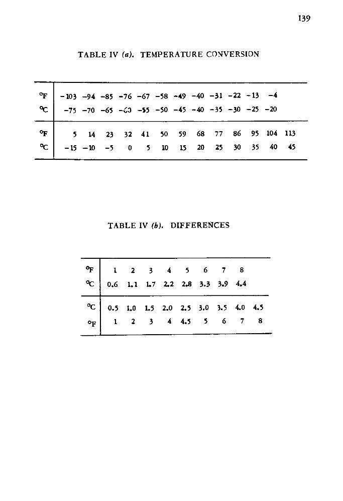
TABLE IV (a). TEMPERATURE CONVERSION
139
°F -103 -94 -85 -76 -67 -58 -49 -40 -31 -22 -13 -4
PC -75 -70 -65 -£0 -55 -50 -45 -40 -35 -30 -25 -20
°F 5 14 23 32 41 50
°C -15 -10 -5 0 5 10
59 68 77 86 95 104 113
15 20 25 30 35 40 45
TABLE IV (b). DIFFERENCES
op
°C12345678
0.6 1.1 1.7 2.2 2.8 3.3 3.9 4.4
°C 0.5 1.0 1.5 2.0 2.5 3.0 3.5 4.0 4.51 2 3 4 4.5 5 6 7 8
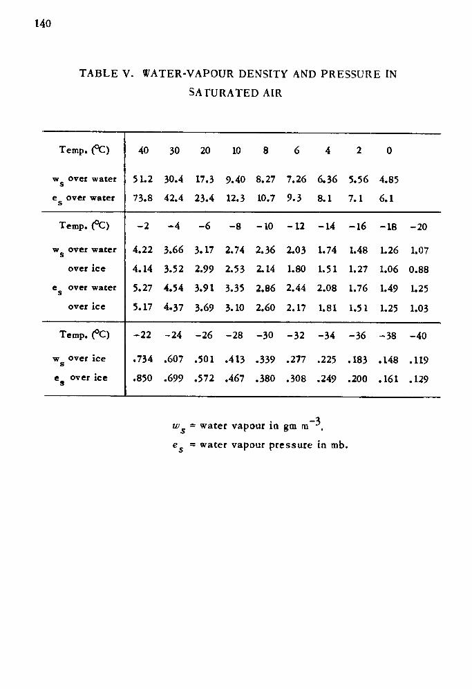
140
TABLE V. WATER-VAPOUR DENSITY AND PRESSURE INSATURATED AIR
Temp. (?C)
w over water
e over water
40 30 20 10 8 0
51.2 30.4 17.3 9.40 8.27 7.26 6.36 5.56 4.8573.8 42.4 23.4 12.3 10.7 9.3 8.1 7.1 6.1
Temp. (°C)
w over water
over ice
e over watersover ice
-2 -4 -6 -8 -10 -12 -14 -16 -18 -20
4.22 3.66 3.17 2.74 2.36 2.03 1.74 1.48 1.26 1.07
4.14 3.52 2.99 2.53 2.14 1.80 1.51 1.27 1.06 0.88
5.27 4.54 3.91 3.35 2.86 2.44 2.08 1.76 1.49 1.25
5.17 4.37 3.69 3.10 2.60 2.17 1.81 1.51 1.25 1.03
Temp. (°C)
w over ice
e over ice
-22 -24 -26 -28 -30 -32 -34 -36 -38 -40
.734 .607 .501 .413 .339 .277 .225 .183 .148 .119
.850 .699 .572 .467 .380 .308 .249 .200 .161 .129
w -3= water vapour in gm tn e = water vapour pressure in mb.
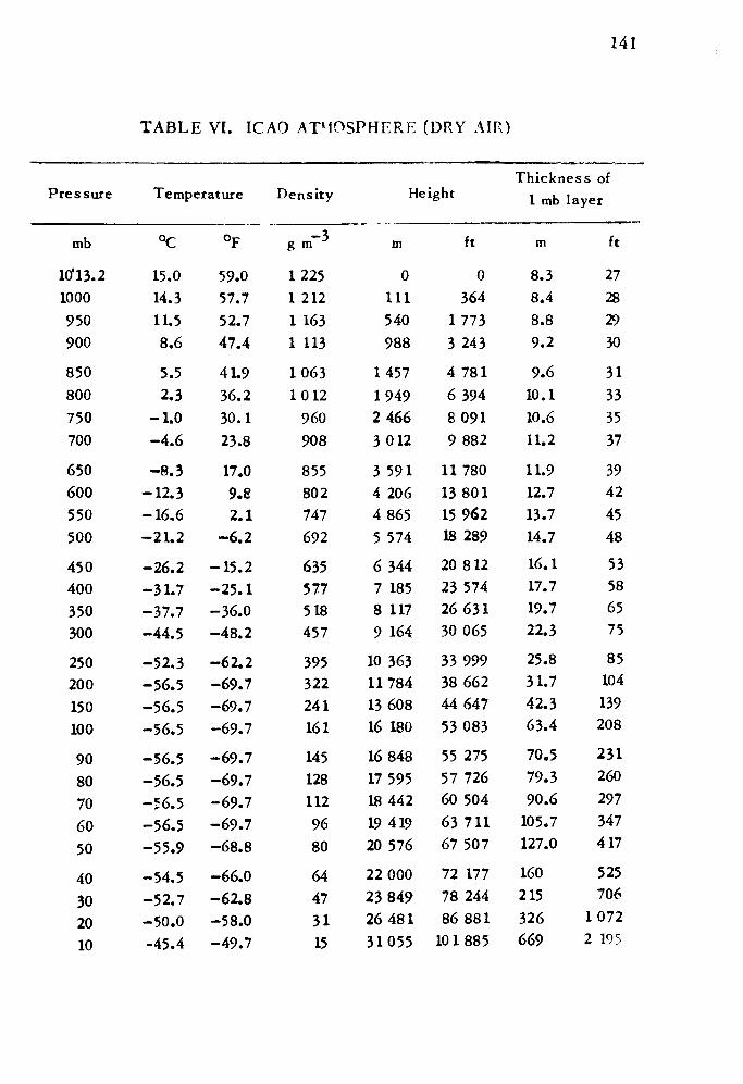
141
TABLE VI. ICAO ATMOSPHERE (DRY AIR)
Pressure
mb
10-13.21000950900
850800750700
650600550500
450400350300
250200150100
9080706050
40302010
Temperature
°C
15.014.311.58.6
5.52.3
-1.0-4.6
-8.3-12.3-16.6-21.2
-26.2-31.7-37.7-44.5
-52.3-56.5-56.5-56.5
-56.5-56.5-56.5-56.5-55.9
-54.5-52.7-50.0-45.4
oF
59.057.752.747.4
4L936.230.123.8
17.09.82.1
-6.2
-15.2-25.1-36.0-48.2
-62.2-69.7-69.7-69.7
-69.7-69.7-69.7-69.7-68.8
-66.0-62.8-58.0-49.7
Density
g m
12251 2121 1631 113
10631012
960908
855802747692
635577518457
395322241161
1451281129680
64473115
Height
m
0111540988
1457194924663012
3 5914 20648655 574
6 3447 1858 1179 164
10 3631178413 60816 180
16 848175951844219 41920 576
22000238492648131055
ft
0364
17733 243
4 7816 39480919 882
11 78013 80115 96218 289
20 81223 57426 63130 065
33 99938 66244 64753083
55 27557 72660 50463 71167 507
72 17778 24486 881
10 1 885
Thickness of 1 mb layer
m
8.38.48.89.2
9.610.110.611.2
11.912.713.714.716.117.719.722.3
25.831.742.363.4
70.579.390.6
105.7127.0
160215326669
ft
27282930
31333537
3942454853586575
85104139208
231260297347417
525706
10722 195
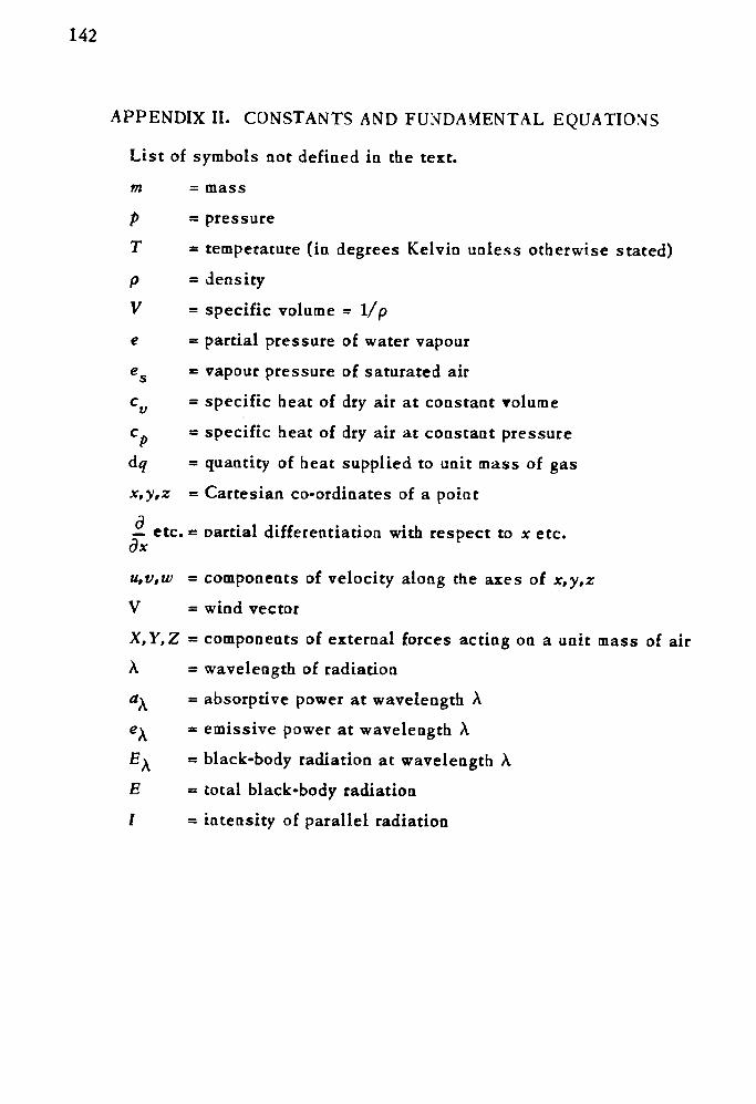
142
APPENDIX II. CONSTANTS AND FUNDAMENTAL EQUATIONS
List of symbols not defined in the text.m = massp = pressureT - temperature (in degrees Kelvin unless otherwise stated)p = densityV = specific volume = 1/pe = partial pressure of water vapoureg «= vapour pressure of saturated aircv = specific heat of dry air at constant volumecp = specific heat of dry air at constant pressuredq - quantity of heat supplied to unit mass of gasx,y,z = Cartesian co-ordinates of a point
_ etc. = oartial differentiation with respect to x etc. dx
u,v,w = components of velocity along the axes of x,y,zV = wind vectorX, Y, Z = components of external forces acting on a unit mass of airA = wavelength of radiationa\ = absorptive power at wavelength Ae\ = emissive power at wavelength AE\ = black-body radiation at wavelength AE - total black-body radiation/ = intensity of parallel radiation
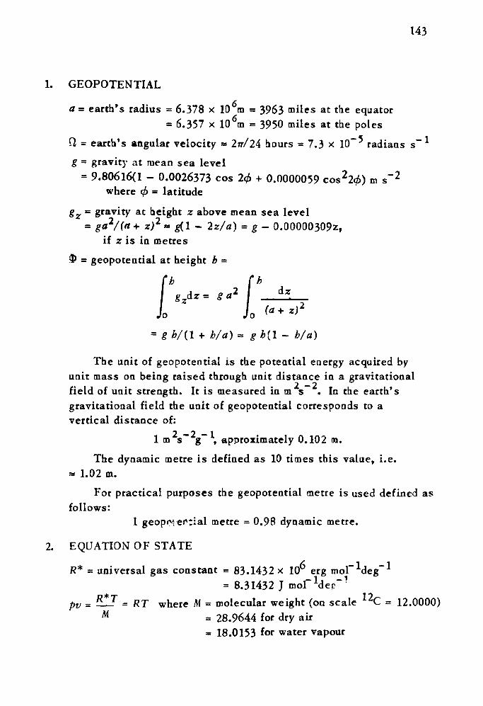
143
1. GEOPOTENTIAL
a = earth's radius = 6.378 x 10 m = 3963 miles at the equator = 6.357 x 10 6m = 3950 miles at the poles
Q = earth's angular velocity » 2rr/24 hours = 7.3 x 10~ 5 radians s g = gravity at mean sea level
= 9.80616(1 - 0.0026373 cos 20 + 0.0000059 cos 220) m s~ 2 where 0 = latitude
gz = gravity at height z above mean sea level= g<* 2/(tt + z) 2 « g(l - 2z/a) = g- 0.000003092,
if z is in metres$ = geopotential at height b =
'h
-1
b/a)« gb(l~ b/a)
The unit of geopotential is the potential energy acquired byunit mass on being raised through unit distance in a gravitational
2. —2 field of unit strength. It is measured in m s .In the earth'sgravitational field the unit of geopotential corresponds to a vertical distance of:
2 2—1 1m s g , approximately 0.102 <n.The dynamic metre is defined as 10 times this value, i.e.
» 1.02 m.For practical purposes the geopotential metre is used defined as
follows:l metre = 0.98 dynamic metre.
2. EQUATION OF STATE
R* = universal gas constant = 83.1432 x 10 erg mol~ deg= 8.31432 J mor^ec" 1
pv = ^U = RT where M = molecular weight (on scale 12C = 12.0000) M = 28.9644 for dry air
= 18.0153 for water vapour
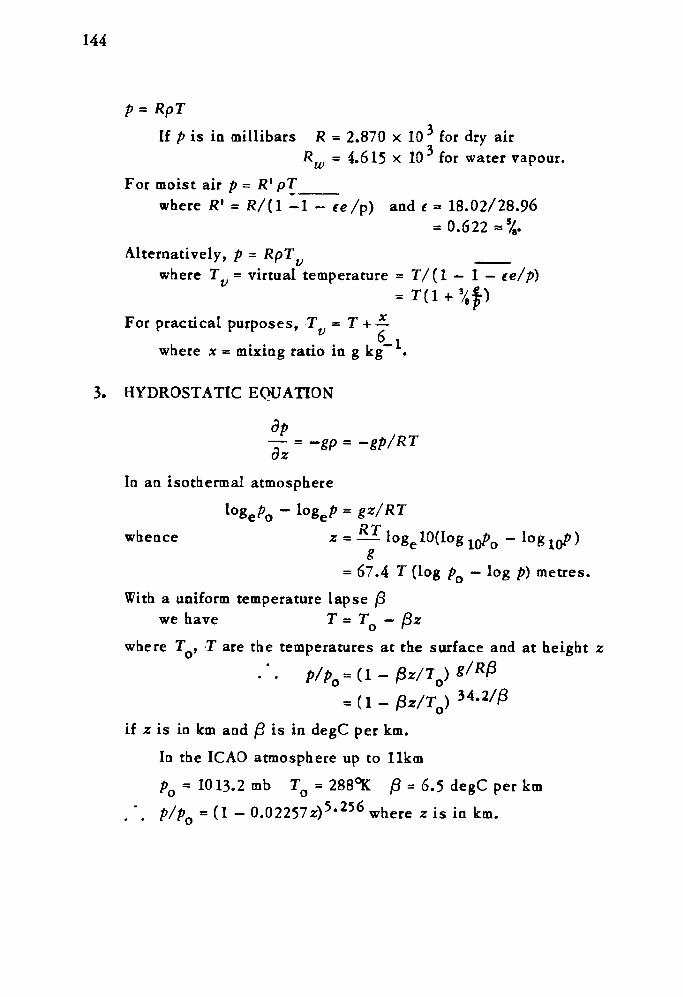
144
p=RpTIf p is in millibars R = 2.870 x 10 3 for dry air
R W = 4.615 x 10 for water vapoFor moist air p = R* pT ___
where /?' = R/(l -1 - ee /p) and f = 18.02/28.96= 0.622 »%.
Alternatively, p = RpTv ___where T = virtual temperature = T/(l — 1 — ce/p)
For practical purposes, T = T + —6«
where x = mixing ratio in g kg" .
3. HYDROSTATIC EQUATION
— = -gp = -az
In an isothermal atmosphere
whence z = —— ioge 10(log wpQ - logg
= 67.4 T (log pQ — log p) metres.With a uniform temperature lapse (3
we have T = T — /8zwhere TQ, T are the temperatures at the surface and at height z
«(l-/3z/T0) 34 ' 2//3
if z is in km and /3 is in degC per km.
In the ICAO atmosphere up to llkm
P0 = 1013.2mb TQ = 288°K 0 = 6.5 degC per km . '. P/P = (1 - 0.02257z) 5 ' 256 where z is in km.
145
In general,
fft., /*&, _R T , P l
PIwhere T is the mean temperature in the layer between p-, and py. This equation establishes the equivalence of thickness lines and mean isotherms.
THERMODYNAMICS
dq = cvdT + pdv = (c^ + R)dT - vdp = cpdT - vdp
cv = 0.7147 x 10⁷ erg g" 1 deg" 1 = 0.7147 x 10³ J kg" 1 deg" 1
c p = 1.0031 x 10⁷ erg g" 1 deg"1 = 1.0031 x 10³ J kg" 1 deg" 1
R - c - c = c(In adiabatic conditions, dq = 0 and hence dp =
-dl,-i ^ = ^=9. dz cP dz c
T CP T cp P y Py- 1/y
. . T/p = constant, or pv^ = constant.
Potential temperature 6 = T(pJp)y~ l/y = T(p/p)°' 2B8
T y P T cp RT cpT
—•2.= c Jog 0 + constant
In adiabatic conditions, with dq = 0, 6 and S are constant.
5. WATER VAPOURmass of vapour .
x = humidity mixing ratio = mass of dry air " P™/Pd
146
_ e //>—e _ fe a ee where ( = 0. ~" R wT/ RT P~* ~P
= 0.622 (See section 2)
= specific bumidity = _____mass of vapour______ = pwmass of dry air + mass of vapour pj + p
ee- 1 + 1/x - p - (1 - €)e p
Tfj = virtual temperature = T/(l - 1 - f e//>) (See § 2)
-!-«*)« IU +
L = latent heat of evaporation
= 597.3 - 0.56T cal g' 1 = (2500.9 - 2.34T) x 10 3 J kg-1 where T is in °C
L {- = latent heat of melting ice
= 79.7 cal g"1 = 333.7 x 10 3 J kg" 1
Clausius-Clapeyron equation is: 1 de_ L fL
o
es dT R^T^
F a saturated adiabatic lapse rate
p+cLes /RT
dry *,i,2 f 2 / DT^ y p + € L es /CpRl
6. EQUATION OF CONTINUITY
In Cartesian co-ordinates
— 1 dp du dv dw -—=--+ — + ——=div V p dt ox By oz
If the vertical co-ordinate is p,
\dxV (or V . V)
147
where = =dt dt dx dz dz
In mid-troposphere the last term • ff, is frequently the largest and,(9 ^ Z
since— £- = — pg» leads to the approximate relationship,dz
p = -
7. EQUATIONS OF MOTION
= -- 2 d/ p dx
d/ p dy
dt p dz
If w is negligible compared with v, and if all external forces except friction are negligible, then
where
are the components of the geostrophic wind V and F^, fy are the horizontal components of the frictional force.
Rearranging, and putting v* = v — v , «' = »—«, thenA,, &u ~ du
/i/ l -^i-F Y -_J* __ -FY dt X dt dt X
j f . dv df' /„' = - 5£ + F = _ _^g_ __ pd/ ^ d/ d/ y
du dv Expanding _ I and — £ in terms of the partial derivatives, the
dt dt
148
equations becomedu udu vdu n wdu da 1
fv < = __ S + ___ | + ___ | 4- ___ | - F v 4- __dt dx dy dz X dt
dv udv vdv wdv dv'/ • 0 O 0 P.I"1 «' » — — s — —— 5 — —— e — —— s -I- Fv — —— .
dt dx dy dz Y dt
The first term in each equation represents the isallobaric acceleration: The components of the isallobaric wind are
Idu I dv and — —_ —
f dt f dt
Further,
1 du 1 d I 1 dp \ 1 d dp =1 I 1 p \ 1 p
= J~dl\^f~dyl ~~L ^jtdt
1 dvwith a similar equation for — — s
/ dt
i.e. the isallobaric wind depends upon the gradient of the isallobars/ **P \ I isopleths of — I\ dt I
The second and third terms in each equation represent the horizontal advective acceleration, V. V» V ; The corresponding wind components
oare
1 /udu vdu \ 1/udv vdv \— f g + S and — — I —— I 4- —— i-\f\dx dy I f\ dx dy I
The fourth terms in each equation represent the components of acceleration arising from vertical motion, the y- and x- components of the wind being
w du w dv_ — £ and — — — i.f dz f dz
The fifth terms represent the frictional forces, while the last terms are the components of the ageostrophic acceleration.
149
On isobaric contour charts where the vertical co-ordinate is pdp dp dz dz I dp \— = — — — = g p — I — = — g p jBy dz dy dy * dz '
hence, from the components of the geostrophic wind
org db g dhu = — — v =- — ,
« f dy * f dx
where b is the height of the pressure surface above datum level.
8. VORTICITYdv du
Vorticity, C. = — — — i.e. the component of spin about a vertical dx dy v av
axis, or, in polar co-ordinates , £ = — + — , where r is the radius ofr dn
curvature of the streamline and n is directed normal to the stream line and is positive to the right of it.
Absolute vorticity £ = £ «- /
Vorticity equation, in simplified form, and related to an isobaric surface, relates the change of vorticity with time to divergence,
or
When div^V is small, in particular at the 'level of non-divergence,'
d/
150
Thus absolute vorticity (£+ /) is conserved following the flow. Northward-moving air acquires an increasing value for /and hence a decreasing value for £. The air must curve anticyclonically following a constant absolute vorticity trajectory. Similarly, southward-moving air must curve cyclonically.
Potential vorticity. If div, V is not small then
_d_ (^\ =0 dt \ A/? /'£+/
or potential vorticity ———= constant, where &p is the pressure
difference between the isentropic surfaces representing the top and bottom of an air column.
Development. In the usual case where
-i(£+/)«-/div v.dt ?
By using this equation near the surface — say at 1000 mb — and at some upper level and subtracting them to obtain the relative divergence it can be shown that
f(divp V - divp VQ ) . - V'l (£ + 2£0)
where V 1 is the thermal wind, VQ the surface wind,£* the vorticity of the thickness pattern and £. the vorticity of the surface pattern and d/ds denotes differentiation along a thick ness line.
If div, V = 0, i.e. the upper level is a level of non-divergence — say at 500 mb — then
i
relating the surface divergence to the thickness pattern.
151
9. RADIATION
Planck's law: Ev = c j/X5(e 2 -1)
where Cj = 3.74 x 10~5 erg cm 2s~ 1 = 374 x 10" 18 J m 2s~ 1
and c2 = 14 385 (im degK = 1.4385 x 10" 2 m degK
Wien's law: Xmax = 2900/T
Kirchoff's law: a\ = e\/E\f oo
Stefan's law:E =
where a = 5.67 x 10~12 W cm"2 deg"4 = 56.7 x 10"9W m"2 deg"4 = 1.35 x 10~12 cal cm"2 deg~4s~1
= 56.7 x 10"9! m~2
Beer's law: I = lQc'\m
where k^ is the absorption coefficient at wavelength X and m is the mass of the absorbing medium
a
Angstrom's formula for downward radiation:
R = aT4(A-B W~ de)
where A = O.&l, B = 0.24, d = 0.052 and e = surface vapour pressure (mb)
Brunt's law: R = o T*(& + b^/e)
where a = 0.44 and b = 0.80
Nocturnal radiation: N = a * — R
— ° —1 Solar constant = 2.00 cal cm *min= 1.395 x 10 3 J m~2s"1
= 1.395
152
10. MISCELLANEOUS CONSTANTS AND RELATIONS
e = 2.7183 Io8ioe = °-43429 Ioge 10 = 2.3026
1 A (angstrom unit) = 10~®cm = 10" /urn = 10~ 10m
1 calorie (at 15°C) = 4.1855 x IO7 erg = 4.1855 J
1 watt = 0.23892 cal s"1 = 14.335 cal min"1 = 1 J s" 1
1 laagley = 1 cal cm"2 = 41.855 x IO3 J m-2
1 millibar = 1000 dyn cm"2 = IO2 N m"2— 2 1 newton (N) = 1 kg m s
1 knot = 1.689 ft s"1 = 1.853 km h" 1 = 0.5148 m s"1
1000 ft min"1 = 9.73 kt = 5.1 m s"1
1 cm s"1 » 3600 gp x 10~3 mb h"1
= 3.2 mb h"1 at 700 mb
= 1.6 mb h"1 at 300 mb
= 0.6 mb h" 1 at 100 mb
Velocity of sound in dry air = \/(y RT) (T in degrees Kelvin)
- 331 V(l + T/273) m s"1 if T is in degrees Celsiusfi ? Area of earth's surface = 510 x 10 km z
Area of ocean surface = 360 x 10b km 2 (70.8% of earth's surface)i< ^
Area of land surface = 150 x 10° km z (29.2% of earth's surface)91 Mass of atmosphere = 5.27 x 10 g
fdu \ 2 II dT\Richardson number Ri - gB/ [ — I where & = — I F •»- —
\ dz I M T \ dz I
c ,5>corer s parameter / = — i — — —t/ 2 U dz
S02640/544855 2400 11/70 GL3917

NOTES