Embed Size (px)
Citation preview

FORECAST EVALUATION OF SMALL NESTED MODEL SETS
Kirstin HubrichEuropean Central Bank
Kenneth D. WestUniversity of Wisconsin
November 2007Last revised February 2009
Abstract
We propose two new procedures for comparing the mean squared prediction error (MSPE) of abenchmark model to the MSPEs of a small set of alternative models that nest the benchmark. Ourprocedures compare the benchmark to all the alternative models simultaneously rather than sequentially,and do not require reestimation of models as part of a bootstrap procedure. Both procedures adjust MSPEdifferences in accordance with Clark and West (2007); one procedure then examines the maximum t-statistic, the other computes a chi-squared statistic. Our simulations examine the proposed proceduresand two existing procedures that do not adjust the MSPE differences: a chi-squared statistic, and White’s(2000) reality check. In these simulations, the two statistics that adjust MSPE differences have mostaccurate size, and the procedure that looks at the maximum t-statistic has best power. We illustrate ourprocedures by comparing forecasts of different models for U.S. inflation.
Keywords: Out-of-sample, prediction, testing, multiple model comparisons, inflation forecasting
We thank Roberto Duncan, Eleonora Granziera and Maria Zucca for research assistance, MichaelMcCracken for supplying the unpublished tables of quantiles referenced in section 3, and RaffaellaGiacomini, participants at the 5th ECB Workshop on Forecasting Techniques, two anonymous refereesand Tim Bollerslev (the editor) for helpful comments. West thanks the National Science Foundation forfinancial support. The views expressed here are not necessarily those of the European Central Bank.
1
1. INTRODUCTION
Forecast evaluation frequently involves comparison of a small set of models, one of which is a
null model nested in the alternative models. There are two broad classes of applications. In one class,
applicable to studies of asset returns, the null model is a martingale difference, perhaps with drift (i.e., a
random walk or random walk with drift for the asset price). Examples include Hong and Lee (2003), who
study exchange rates, and Sarno et al. (2005), who study interest rates; each paper compares a random
walk to a half dozen or so other models. In the second class of applications, the null model sometimes
relies on stochastic predictors, typically via a univariate autoregression. Examples include Billmeier
(2004), who compares a univariate autoregression (AR) to four other models that include four different
measures of the output gap, and Hubrich (2005) and Hendry and Hubrich (2006, 2007), who compare
univariate forecasts of aggregate inflation to a couple of other forecast models that add disaggregate
components of inflation to the univariate model. This class of applications is important at policy
institutions or for policy observers where it is of interest to compare forecasts from different models in a
suite of models built to account for different aspects of the economy.
Our aim in this paper is to propose and evaluate procedures for performing inference about
equality of mean squared predictions errors (MSPEs) in applications, such as these, that involve a small
number of models. We do not have a precise definition of “small.” But, loosely, the idea is that the
number of alternative models m is much less than the sample size T.
There are at least two existing procedures. Both use a m × 1 vector whose elements consist of the
difference between the MSPE of the null model and the MSPE of one of the alternative models. To test
the null of equality of MSPEs across the models, one approach is to conduct the chi-squared test that is
the straightforward generalization of the Diebold and Mariano (1995) and West (1996) (DMW) statistic
that is used to compare a pair of models. This chi-squared statistic was used in West et al. (1993) and
West and Cho (1995). It is referenced in our paper as “χ2 that does not adjust MSPE differences” or “χ2

2
(unadj.);” the reason for the qualification “unadjusted” will become clear shortly. Under our null
hypothesis, however, this statistic is flawed in terms of both size and power. In terms of size: under a
reasonable set of technical assumptions, the statistic is unlikely to be well-approximated by a chi-squared,
because the vector of MSPE differences is not centered at zero, even under the null. We explain this
point in section 2 below. In terms of power: as argued by Ashley et al. (1980), the alternative in question
is one-sided. So even if the statistic is adjusted so as to be centered at zero under the null, a large
chi-squared value can reflect extreme behavior in either tail of the underlying distribution, and thus this
statistic potentially has poor power.
A second procedure, or perhaps we should say class of procedures, is to obtain critical values on
the distribution of the vector of MSPE differences via simulation. One such possibility is White’s (2000)
reality check. While White (2000) proposed his procedure in the context of applications with many (m .
T) rather than a small (m << T) number of nested models, the technique has also been applied to small
sets of nested models (Hong and Lee (2003)). A possible problem is that White’s procedure might not
accurately account for dependence of predictions on estimated regression parameters (a key aspect of the
computational appeal of White’s procedure is that it does not require reestimation of models during
bootstrap repetitions). Under our null, this problem is relevant as well to Hansen’s (2005) test for
superior predictive ability.1 Alternatively, one could bootstrap in a fashion that includes reestimation of
models (e.g., Rapach and Wohar (2006)). Such a bootstrap has been found to work well (Clark and
McCracken (2006), Clark and West (2007)). Nevertheless, in our own applied work, and, we presume, in
the applied work of some others, it will at times be desirable to have procedures that do not require
repeated reestimation of models.
In this paper, we develop two closely related procedures for multi-model comparisons in which
the alternative models nest a benchmark model. Key features are that we take estimation uncertainty into
account, and that we use standard or easily computed critical values. We compare our proposed

3
procedures to the unadjusted chi-squared and White’s (2000) reality check via simulations.
Let model 0 denote the benchmark model, and number the alternative models 1 to m. Our main
proposal involves two steps: (a) adjust the difference between the MSPE of the benchmark model and
each of the alternative models as in Clark and West (2007). The result will be m “MSPE-adjusted”
t-statistics, one of which compares model 0 to model 1, the second of which compares model 0 to model
2, ..., the last of which compares model 0 to model m. Next, (b) conduct inference on the largest of the m
adjusted t-statistics via the distribution of the maximum of correlated normals. In our tables, this is
called “max t-stat (adj.),” where the qualifier “adj.” signals use of adjusted MSPEs.2
In step (a), the adjustment of the MSPE differences is intended to center the vector at zero, under
the null. Step (b) respects the one-sided nature of the alternative, and is intended to lead to good power.
When there are only m=2 alternative models in addition to the benchmark model, as in some of the
simulations presented below, critical values for this test vary with a single parameter, namely, the
correlation between the two t-statistics. We include a table that presents critical values for 10% and 5%
tests, for a crude grid of possible correlations. We supply detailed critical values for a fine grid of
correlations in a not-for-publication appendix. When the number of alternatives is m>2, critical values
for this statistic are easily obtained by a simple procedure: (1)draw many times from an m dimensional
normal distribution whose variance-covariance matrix is set to the sample variance-covariance matrix of
the MSPE-adjusted t-statistics; (2)use the quantiles of maximum of the m correlated values.
Our second proposal is to compute a conventional χ2(m) statistic from the m × 1 vector of Clark
and West (2007) MSPE-adjusted values. Since this procedure uses the adjusted differences, we
conjecture that it will be well-sized. But since it uses both tails of the distribution, it is likely to have less
power than does the procedure that considers the maximum of the individual t-statistics. This procedure
is denoted “χ2 (adj.)” in our tables and is sometimes referenced in our text as “χ2 statistics based on the
adjusted MSPE differences.”

4
In our simulations, we find the following, for one step ahead predictions. The max t-stat (adj.)
statistic is slightly undersized, the χ2 (adj.) statistic is slightly oversized. The χ2 statistic used in West et
al. (1993) and West and Cho (1995)–referenced as “χ2 (unadj.) in our tables, because it is computed from
the usual rather than from adjusted MSPE differences–is somewhat, and for small sample sizes grossly,
oversized; the reality check statistic is somewhat, and for small sample sizes grossly, undersized. In terms
of power (not adjusted for size), as expected, max t-stat (adj.) has higher power than the χ2 (adj.) statistic
(although the differences are found not to be large); the χ2 (adj.) statistic in turn has greater power than
either the reality check or the χ2 (unadj.) statistics (often substantially higher power, as it turns out).
We close our introduction by noting that we do not attempt to explain or defend the use of out of
sample analysis. As is usual in out of sample analyses, our null is one that could be tested by
conventional in-sample tools, in our case by testing whether certain regression coefficients are zero. Out
of sample analyses may or may not have power relative to in sample analyses. See, for example, Inoue
and Kilian (2004, 2006) and Hansen (2008) for theoretical comparisons of in and out of sample analysis.
Our aim is not to argue for out of sample analysis, but to supply tools to researchers who have concluded
that out of sample analysis is informative for the application at hand.
Section 2 motivates our two new procedures. Section 3 gives a precise statement of the
environment and the statistics we compute. While the statement is precise, the argument is informal: we
do not prove any theorems, but instead refer the reader to other literature. Section 4 gives an overview of
our simulation set-up. Section 5 presents simulation results. Section 6 presents an empirical example.
Section 7 concludes. An appendix, available from the authors, contains some additional simulation
results omitted from the paper to save space.
2. OVERVIEW AND INTUITION
We propose two tests to compare a parsimonious benchmark model to a set of m > 1 other models
5
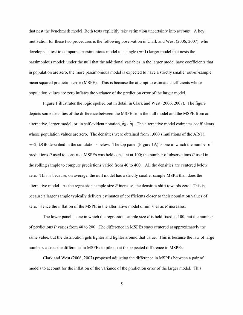
that nest the benchmark model. Both tests explicitly take estimation uncertainty into account. A key
motivation for these two procedures is the following observation in Clark and West (2006, 2007), who
developed a test to compare a parsimonious model to a single (m=1) larger model that nests the
parsimonious model: under the null that the additional variables in the larger model have coefficients that
in population are zero, the more parsimonious model is expected to have a strictly smaller out-of-sample
mean squared prediction error (MSPE). This is because the attempt to estimate coefficients whose
population values are zero inflates the variance of the prediction error of the larger model.
Figure 1 illustrates the logic spelled out in detail in Clark and West (2006, 2007). The figure
depicts some densities of the difference between the MSPE from the null model and the MSPE from an
alternative, larger model, or, in self evident notation, ^σ20 - ^σ2
1. The alternative model estimates coefficients
whose population values are zero. The densities were obtained from 1,000 simulations of the AR(1),
m=2, DGP described in the simulations below. The top panel (Figure 1A) is one in which the number of
predictions P used to construct MSPEs was held constant at 100; the number of observations R used in
the rolling sample to compute predictions varied from 40 to 400. All the densities are centered below
zero. This is because, on average, the null model has a strictly smaller sample MSPE than does the
alternative model. As the regression sample size R increase, the densities shift towards zero. This is
because a larger sample typically delivers estimates of coefficients closer to their population values of
zero. Hence the inflation of the MSPE in the alternative model diminishes as R increases.
The lower panel is one in which the regression sample size R is held fixed at 100, but the number
of predictions P varies from 40 to 200. The difference in MSPEs stays centered at approximately the
same value, but the distribution gets tighter and tighter around that value. This is because the law of large
numbers causes the difference in MSPEs to pile up at the expected difference in MSPEs.
Clark and West (2006, 2007) proposed adjusting the difference in MSPEs between a pair of
models to account for the inflation of the variance of the prediction error of the larger model. This

6
adjustment centers the difference at zero, and is intended to produce a test statistic with good size. We
will give a precise description of this adjustment in the next section.
It may be shown that by centering the difference in MSPEs at zero, the adjustment transforms the
difference in MSPEs into an encompassing statistic (Clark and West (2007, p297)). The two ways of
writing the statistic–i.e., adjusted difference in MSPEs, or encompassing–are algebraically identical. We
prefer the “adjusted difference in MSPEs” way of writing the statistic because in our view this makes it
easier to see how the statistic compares to the conventional DMW statistic for equal MSPE. Readers
who prefer the encompassing interpretation should note that one of our contributions is to provide an
encompassing test for small model sets, rather than a pairwise one as in previous literature.3
3. ECONOMETRIC PROCEDURE
We suppose that there are m + 1 models under consideration. Each of the models is to be used to
predict a scalar yt. For expositional clarity, we assume in this section that m = 2 and that the forecast
horizon is one step ahead. (Generalization to arbitrary m is straightforward. As well, the procedures about
to be described extend immediately to multistep forecasts using the direct method, though, as noted
below, the theoretical justification for our procedure does not always extend.) Model 0 is a parsimonious
benchmark model nested in alternative models 1 and 2. For example, model 0 might be a univariate
autoregression in yt, models 1 and 2 bivariate and trivariate vector autoregressions in which the right hand
side variables include lags of yt. Alternatively, model 1 might add lags of a second variable while model
2 instead adds lags of a third variable. Thus, while model 0 is nested in models 1 and 2, model 1 may or
may not be nested in model 2 and model 2 may or may not be nested in model 1.
3.1 Mechanics
Write the null and two alternative models as

7
(3.1) yt = X0tNβ*0 + e0t,
yt = X1tNβ*1 + e1t,
yt = X2tNβ*2 + e2t.
By assumption X0t is a strict subset of X1t and of X2t . Our dating convention allows (indeed, presumes)
that for each model, Xit is observed prior to period t. For example, we might have X0t = (1 yt-1)N,
X1t = (1 yt-1 yt-2)N, X2t = (1 yt-1 zt-1)N for some z that is observed in period t-1 (or X2t =
(1 yt-1 yt-2 yt-3 yt-4)N–again, models 1 and 2 may or may not be nested in one another). It is possible that
X0t/0, i.e., that the null model presumes that yt is white noise. The β*’s are understood to be linear
projections, with eit by construction orthogonal to Xit. The assumption of linearity is for expositional
convenience; methods such as nonlinear least squares are allowed by our test procedures.
Under the null, the coefficients on the additional regressors in X1t and X2t are zero. (In the
example, just given, this means that the coefficients on yt-2 in X1t and on zt-1 in X2t are zero.) That is,
under the null, X0tNβ*0 = X1tNβ
*1 = X2tNβ
*2 and e0t = e1t = e2t. Under the alternative, at least one of the
additional regressors in X1t and/or X2t has a nonzero coefficient. For i = 0,1,2, let σ2i / Ee2
it denote the
population variance of the forecast error.4 We have
(3.2) H0: σ20 - σ2
1 = 0, σ20 - σ2
2 = 0; HA:max(σ20 - σ2
1, σ20 - σ2
2) > 0.
Note that the alternative is one-sided. This is in accordance with Ashley et al. (1980) and a long list of
subsequent studies. If, indeed, one or more of the coefficients in β*1 or β*
2 are nonzero, then σ21 or σ2
2 must
be less than σ20.
Define the following notation, putting aside for the moment details such as whether a rolling or
recursive scheme is used to generate prediction errors:
(3.3)(a)^βit: an estimate of β*i computed using period t or earlier data, i = 0,1,2;

8
(b) ^yit+1: the one step ahead forecast from model i, (i = 0,1,2), ^yit+1 = Xit+1N^βit;
(c) ^eit+1:one step ahead prediction error from model i (i = 0,1,2), ^eit+1/yt+1 - ^yit+1;
(d) P: the number of predictions and prediction errors;
(e) ^σ2i: mean squared prediction error (MSPE) from model i (i = 0,1,2), ^σ2
i / P -13t^e2
it+1;
(f) ^σ2i-adj: Clark and West’s (2007) adjusted MSPE for models i = 1, 2,
^σ2i-adj = ^σ2
i - P -13t(
^y0t+1 - ^yit+1)2;
(g) ^fit+1/ ^e20t+1 -
^e2it+1 + (
^y0t+1 - ^yit+1)2 (i = 1,2);
(h) 'f i: the adjusted difference in MSPEs between model i (i = 1,2) and model 0,
'f i = ^σ20 - ( ^σ2
i-adj) = P -13t ^fit+1;
(i) ^vi: an estimate of a long run variance computed using autocovariances of ^fit+1 (i = 1,2) (typically,
for one step ahead predictions, ^vi = sample variance of ^fit+1);
(j) P ½'f i / : for i = 1,2, the MSPE-adjusted t-statistic.$vi
Clark and West (2006, 2007) argue that for the purpose of comparing model 0 to model 1, one
can compute the MSPE-adjusted t-statistic P ½'f 1/ and use standard normal critical values, i.e., one can$v1
assume P ½'f 1/ -A N(0, 1); similarly, one can compare model 0 to model 2 via P ½'f 2/ -A N(0, 1). $v1 $v2
This motivates us to assume the following when we conduct inference:
(3.4) P ½ -A N(0, Ω), Ω / .
f
vf
v
1
1
2
2
$
$
⎛
⎝
⎜⎜⎜⎜⎜
⎞
⎠
⎟⎟⎟⎟⎟
11ρ
ρ⎛⎝⎜
⎞⎠⎟
Our first proposed test statistic is as follows. Let ^z be the larger of the two t-statistics
(3.5) ^z = max[P ½'f 1/ , P ½'f 2/ ] / max t-stat (adj.).$v1 $v2
Consider a test at the α level of significance. Let gz(z) denote the density of the larger of two standard
normal random variables with correlation ρ. Let cα(ρ) be such that Ic-α4
(ρ)gz(z)dz = 1 - α. We propose

9
rejecting the null in favor of the alternative if ^z > cα(^ρ), where ^ρ is the sample correlation between the two
t-statistics 'f 1/ and 'f 2/ .$v1 $v2
To use this result requires knowledge of the quantiles of gz(z) . For the case of m=2, the density
is presented in Cain (1994) and Ker (2001). We use this density to solve numerically for the value of c
such that Ic-4 gz(z)dz = 0.90 or Ic
-4 gz(z)dz =0.95. Table 3.1 has the results. The entries for positive ρ may
also be found in Gupta et al. (1973). The entries for ρ = -1, ρ = 1 and ρ = 0 are intuitive or familiar. Let z1
and z2 denote two standard normal variables. If ρ = -1, then z1 = -z2 and prob[max(z1, z2) > c] = prob[z1 > c]
+ prob[z1 < -c], so a 10% critical value is c = 1.645 (since prob[z1 > 1.645] + prob[z1 < -1.645] = .10). If
ρ = 1, then z1 = z2 and prob[max(z1, z2) > c] = prob(z1 > c) so a 10% critical value is c = 1.282. If ρ = 0,
familiar results on order statistics from independent observations tell us that the 10% critical value
satisfies Φ(c)2 = .90, yielding the value of c = 1.632 given in the table. The critical values fall
monotonically as ρ rises, initially with little change, but with an accelerating decline as ρ nears 1.
The second of our two new procedures computes a chi-squared statistic from the vector of
adjusted MSPE differences. Define:
(3.6)(a) ^ft+1 / ( ^f1t+1, ^f2t+1)N / (^e20t+1 -
^e21t+1 + (
^y0t+1 - ^y1t+1)2, ^e2
0t+1 - ^e2
2t+1 + (^y0t+1 -
^y2t+1)2)N,
(b) ^V / P-13t(^ft+1 -
'f )(^ft+1 - 'f )N.
Our second proposed test statistic is
(3.7) χ2 (adj.) / P'f N ^V -1'f .
We evaluate (3.7) using χ2(2) critical values; the diagonal elements of ^V are ^v1 and ^v2, defined in (3.3(i)).
We use simulations to compare our two new procedures to two existing procedures, a χ2 statistic
that uses unadjusted MSPEs, and White’s (2000) reality check.
•χ2 using unadjusted MSPEs: Use “~” on top of a quantity to define MSPE differences that are not

10
adjusted as in Clark and West (2007). This leads to the χ2 statistic proposed in West and Cho (1995):
(3.8)(a) ~f it+1: ^e20t+1 -
^e2it+1 (i = 1,2);
(b) G~f i = ^σ20 - ^σ2
i = P -13t ~f it+1 (i = 1,2);
(c) ~f t+1 / (~f1t+1, ~f2t+1)N / (^e20t+1 -
^e21t+1, ^e2
0t+1 - ^e2
2t+1)N;
(d) G~f / (G~f1, G~f2)N = P-13t ~f t+1;
(e) ~V /P-13t (~f t+1 -
G~f)(~f t+1 - G~f)N;
(f) χ2 (unadj.) / PG~fN~V -1G~f .
We evaluate (3.8(f)) using χ2(2) critical values. For clarity, we observe that the adjusted and unadjusted
MSPE differences are related via: i’th adjusted MSPE difference = i’th unadjusted MSPE difference +
P-13t(^y0t+1 -
^yit+1)2.
•White’s (2000) reality check. When comparing nested models, the null in White (2000) is the one
considered here–equality of MSPEs. See the discussion at the end of section 3.3.
3.2 Mechanics, more complex settings
For the case of m=2 alternative models, a not-for-publication appendix available on request
extends the coarse grid supplied in Table 3.1 by providing critical values for steps in ρ of 0.01. More
generally, for any m, one can compute the p-value of a “max MSPE-adj. t-statistic” by a simple
simulation. One computes m MSPE-adjusted t-statistics, and constructs an m × m matrix ^Ω; here, the i, j
element of ^Ω is the sample correlation between ^σ20 - (
^σ2i-adj) and ^σ2
0 - (^σ2
j-adj). One then does a series of
draws (say, 50,000 draws)5 on a N(0, ^Ω) random vector, and, for each draw, saves the largest of the m
elements of that draw’s random vector. The p-value for sample maximum MSPE-adjusted statistic is
computed from the distribution of maxima from the simulation.
The statistics defined in (3.7) and (3.8(f)) generalize immediately to an environment with m > 2.
All the statistics we consider also generalize immediately to multistep forecasts executed using

11
the direct method. ^V (3.6(b)) and ~V (3.8(e)) become estimates of a long run variance; the diagonal
elements of ^V are used in the denominator of the MSPE-adjusted statistics, and the off-diagonal
correlations in ^Ω are computed from the off–diagonal elements of the long run variance estimate ^V. With
these changes, the formulas above are applicable.
3.3 Theoretical justification
As a formal matter, the max t-stat (adj.) and χ2 (adj.) procedures require that m × 1 vector P ½'f be
asymptotically normal with a variance that can be estimated in standard fashion. Under technical
conditions such as in Giacomini and White (2006), it is straightforward to show that this holds when
(a) the null model posits that yt is a martingale difference (i.e., X0t / 0, ^y0t+1 / 0 for all t), and (b) rolling
samples are used to generate the regression estimates.6 Under the conditions just stated, asymptotic
normality also follows for multistep prediction errors if predictions are made using the direct method.7
Alternatively, under the technical conditions of Clark and McCracken (2001), asymptotic
normality follows if P is very small relative to the number of observations R used in the first regression
sample used to estimate the β*’s. The precise requirement is that P/R 6 0 as the total sample size grows.
This result holds for both recursive and rolling samples, and does not require that the null model be a
martingale difference. It does require one-step ahead predictions. Extension to multistep predictions has
been worked out only in special cases (Clark and McCracken (2005)).
The conditions of the previous two paragraphs do not by any means span the environment of
applications that compare small sets of nested models. But the argument of Clark and West (2007)
suggests that the quantiles of the right tail of the t-statistics described above will be approximately those
of a standard normal in a wide range of environments. Hence the max t-stat (adj.) procedure should yield
tests that are approximately accurately sized. In particular, using numerical methods, Clark and
McCracken (2001) have tabulated critical values for the adjusted t-statistic, which they call “enc-t”.
These critical values assume that P, R 6 4. The critical values depend on the limiting value of P/R, on the

12
regression scheme (rolling vs. recursive) and on the number of extra regressors in the larger model (i.e.,
on the difference between the dimension of X1t and X0t or between X2t and X0t). But apart from a handful
of exceptions, for all tabulated values of P/R and the number of extra regressors, the critical values obey
the following inequalities: .90 quantile # 1.282 # .95 quantile # 1.645 # .99 quantile. For a standard
normal, the .90 quantile is of course 1.282 and the .95 quantile is 1.645. Hence t-tests using standard
normal critical values will be somewhat undersized. Our presumption is that the same will apply to the
max t-stat (adj.) procedure.
Rationalization of χ2 (adj.) requires that the quantiles of the left as well as the right tails of the
MSPE-adj. statistics are approximately those of a standard normal. Tables of quantiles of the MSPE-adj.
t-statistics published on Todd Clark’s web page, and additional unpublished tables, indicate that, apart
from a handful of cases,
(3.9) 0.02 < prob [square of t statistic (adj.) > 1.962] < 0.10,
0.06 < prob [square of t statistic (adj.) > 1.6452] < 0.15.
The handful of exceptions to the above inequalities would all be eliminated were we to slightly increase
the 1.6452 in the second line to 1.662. Hence, were we to apply our χ2 (adj.) statistic to an example with
m = 1 (which we have not done), we expect the size of tests computed using the standard critical values
for a χ2(1) to be roughly right.
Under any of the conditions described above, χ2 (unadj.), the statistic defined in (3.8(f)), will not
be correctly sized. This is because of the miscentering depicted in Figure 1.8
We close this section with a brief comparison of our procedure to those proposed in White (2000)
and Hansen (2005). We observe first that White’s (2000) procedure relies on raw rather than adjusted
differences in MSPEs. Hence whether one follows a bootstrap procedure (as preferred by White and, we
believe, others implementing the reality check), or a certain Monte Carlo Reality Check described by

13
White (2000, p1103) (which requires a simulation similar to the one described in the first paragraph of
section 3.2), the resulting test statistic will be different from ours.
A second point is that White’s null (in our notation) is Ef(β*) # 0 (White (2000, p1099)). Here,
Ef(β*) is the m×1 vector (σ20-σ2
1, σ20-σ2
2, ..., σ20-σ 2
m)N. White’s procedure has been applied to both nested and
nonnested model comparisons. 9 But in the context of nested models–which is the relevant context for
our paper–the differences in population MSPEs is zero. Thus, in our context White’s null simplifies to
strict equality: Ef(β*) = 0. We note as well that in the related context of Hansen (2005), a central
innovation relates to handling models whose predictive ability is strictly worse than model 0. But, once
again, in our context (nested models, and a null of strict equality) this innovation is not relevant for size.10
4. SIMULATION OVERVIEW
We completed simulations on two classes of data generating processes. To conserve space, we
report results from only one. This DGP is motivated by the macroeconomic literature on forecasting
inflation, and generates the predictand via an AR(1) process. A second set of simulations is reported in
the appendix. It is motivated by the finance literature on forecasting changes in asset prices, and assumes
the predictand is white noise.
4.1 AR(1) DGP
These data generating processes used in our simulations are motivated by the use of disaggregate
data to forecast an aggregate (Hubrich (2005), Hendry and Hubrich (2006, 2007)) in the literature. There
is an aggregate yt that is the sum of several disaggregate series. We report results when “several” is three
and when “several” is four. We present algebra here for the simpler case of “three,” with obvious
generalization to a larger number of disaggregates. When the aggregate is the sum of three disaggregate
components,
(4.1) yt = y1t + y2t + y3t.

14
We consider m=2 alternative models in addition to the benchmark. The benchmark, model 0, is a
univariate autoregression in the aggregate yt; model i, i=1,2 (or i=1,...,4 for m=4) adds a lag of yit as a
right hand side variable:
(4.2) yt = const. + β*10 yt-1 + e0t / X*
0tNβ*0 + e0t,
yt = const. + β*1iyt-1 + β*
2iyit-1 + e1t / X*itNβ
*i + e*
it, i=1,2.
We specify the data generating processes in terms of the disaggregates. When m=2, we assume
that (y1t, y2t, y3t)N follows a VAR of order 1 with 3 × 3 matrix of autoregressive parameters Φ, and zero
mean i.i.d. normal disturbances Ut / (u1t u2t u3t)N,
(4.3) Yt / (y1t, y2t, y3t)N = μ + ΦYt-1 +Ut , EUtUtN = I3.
Throughout, the mean vector μ was set to (1, 1, 1)N.
When examining size properties, we ensure that the three models in (4.2) have equal MSPE by
specifying Φ to be diagonal with common parameter φ on the diagonal.11 That is, each disaggregate
follows a univariate AR(1) with common parameter φ:
(4.4) yit = 1 + φyit-1 + uit, |φ| < 1, i = 1,2,3
Y yt = 3 + φyt-1 + et, et = u1t + u2t + u3t, Ee2t = 3.
As indicated in (4.4), it follows that yt also follows an AR(1) with parameter φ. The baseline simulations
set φ = 0.5. This process is motivated by empirical applications involving aggregate inflation and its
disaggregate components.
In (4.3), the aggregate will be Granger caused by one of the disaggregates once we depart from
the specification (4.4). In simulations reported below, for evaluation of power for the case of m=2, we
set

15
(4.5) Φ = .05 0 6 00 4 0 3 00 0 05
. .. .
.
−−⎛
⎝
⎜⎜⎜
⎞
⎠
⎟⎟⎟
In such a setting, the univariate process for the aggregate yt is an ARMA(3,2). The eigenvalues of Φ are
0.5, -0.1 and 0.9. Two components that depend on each other might be commodities and services
inflation, while there is a third component (such as food or energy inflation) that shows less
interdependence with the other two components on average.
For the size simulations of the 5-model comparison (m=4) we extend (4.4) to include i=1,…,4
disaggregate components again with φ = 0.5. For the power simulations in case of m=4 we set
(4.6) Φ =
0 5 0 6 0 00 4 0 3 0 00 0 0 3 00 0 0 0 3
. .. .
..
−−⎛
⎝
⎜⎜⎜⎜
⎞
⎠
⎟⎟⎟⎟
The univariate process of the aggregate then follows an ARMA(4,3) with eigenvalues 0.9, -0.1, 0.3, 0.3.
In all simulations reported here, predictions are made using the regressions given in (4.2). In
simulations related to size, these regression specifications are correct in that the regression disturbance /
forecast error is white noise. In simulations related to power, these specifications are incorrect in that the
regression disturbance / forecast error is serially correlated.
4.2 Some details
An overview of our procedures (additional detail is available in a not-for-publication appendix
available from the authors): Our simulations rely on 1000 replications, with all shocks i.i.d. normal
random variables. We report results from rolling samples, for nominal .10 tests. Results for recursive
samples and for nominal .05 tests are reported in the additional appendix. These are qualitatively similar
to the results reported here.
We report results for the following four statistics.
a. Max t-stat (adj.). For m=2 alternative models, we flag rejections by rounding ^ρ to the nearest tenth and

16
using the critical values such as those given in Table 1 (the complete set of critical values is in the not for
publication appendix). For m=4, we use the procedure described in section 3.2, with critical values
determined by 50,000 draws.
b.,c. χ2 (adj.), χ2 (unadj.): rejections flagged using standard χ2 critical values, e.g.., 4.61 for 10% tests
when m=2.
d. Reality check: The Bootstrap Reality Check procedure described in White (2000) was followed, which
means in particular that we use unadjusted differences in MSPEs. We used the stationary bootstrap of
Politis and Romano (1994), with the parameter that White (2000) calls q set to 0.5. The number of
bootstrap repetitions in each simulation sample was 1000.
We report results for 12 combinations of R (rolling regression size / size of smallest recursive
sample) and P (number of predictions): R = 40, 100, 200 and 400, with each value of R paired with
P = 40, 100 and 200. These sample sizes for DGP 1 reflect typical monthly and quarterly values for
macro data.
5. SIMULATION RESULTS
Table 2 has the results of the simulations, for one step ahead predictions.
We find that “max t-stat (adj.)” is modestly undersized. Across the 24 entries in the table, the
median value is 0.071, the maximum 0.100, the minium 0.043. This is consistent with the modest
undersizing predicted by the Clark and McCracken (2005) univariate asymptotics and the simulation
results in Clark and West (2007). There does not appear to be a consistent pattern for which entries are
closer rather than farther from 0.10. In particular, we do not find consistent improvements as P increases
for given R (as is suggested by Clark and West’s (2007) asymptotics) or when P/R is very small (as is
suggested by the different Clark and McCracken ( 2001) asymptotics). A bit of good news is that size is
about the same for larger as for smaller values of m.

17
While not reported in the table, it is worth mentioning that we also analyzed the maximum
t-statistic computed from unadjusted MSPE differences. As in Clark and West (2006, 2007) for m=1, this
statistic was quite undersized under the null, and displayed very poor power under the alternative. For
example, for m=2, P=400, size, the entries for the four values of R were: 0.0, 0.004, 0.012, 0.015 (as
compared to the Table 2 values of 0.1, 0.069, 0.060, 0.043 for the max t-stat (adj.)).
χ2 using the adjusted difference in MSPEs (i.e, “χ2 (adj.)”) is modestly oversized. The median of
the 24 values for χ2 (adj.) is 0.120. Size improves as P gets larger.
χ2 using the unadjusted difference in MSPEs (i.e, “χ2 (unadj.)”): this statistic is modestly
oversized in most entries, grossly oversized for R=40. The extreme example of the latter is a size of 0.505
for R = 40, P = 200, m=4. For larger values of P and R, χ2 (unadj.) is slightly oversized relative to χ2
(adj.).12 This is consistent with Figure 1A: for rolling samples, the mis-sizing is worse for bigger P,
holding R fixed. The median of the 24 values for χ2 (unadj.) is 0.160; all 24 entries are above 0.100.
The reality check is grossly undersized. The median size is 0.022; three of the entries are
identically zero, indicating that not a single one of the simulation samples led to a rejection; the largest
size (for R = 400, P = 40, m=2) is 0.072. Performance shows a distinct pattern of improving as P/R falls
(i.e., moving from right to left in a given row in the table, or bottom to top in a given column). The fact
that the reality check works better for small values of P/R is consistent with the technical conditions in
White (2000), which include the requirement that P/R 6 0 at a certain rate. That the reality check is
undersized is consistent with the simulations in Hansen (2005) and Clark and McCracken (2006).
Table 3 has results for power. This is raw and not size adjusted power (though we note that under
the P/R 6 0 asymptotics referenced in section 3.3, all our statistics are correctly sized asymptotically). As
expected, max t-stat (adj.) has greater power than does χ2 (adj.). Since max t-stat (adj.) is undersized and
χ2 (adj.) is oversized (see Table 2), the discrepancy in power would be greater had we reported
size-adjusted power. For smaller P or R, the reality check has considerably less power than do the other

18
two statistics. For example, for R = 40, power for the reality check is in each case less than half that for
max t-stat (adj.) and χ2 (adj.). Poor power for the reality check was also found in Hansen (2005). Power
for χ2 (unadj.) lies between that for χ2 (adj.) and the reality check.
We conclude that from the perspective of size, max t-stat (adj.) and χ2 (adj.) are about
comparable, with one being slightly undersized, the other slightly oversized. From the point of view of
power, max t-stat (adj.) is slightly preferable.
6. FORECASTING AGGREGATE U. S. INFLATION
In this section, we analyze empirically different methods of forecast accuracy evaluation for a
small set of models that nest the benchmark, including the tests we proposed. The series we forecast is
aggregate inflation, as measured by the US CPI. We present two empirical applications. In the first, we
investigate whether including disaggregate inflation components in the aggregate model does improve
over forecasting the aggregate only using past aggregate information. The second application also
includes models with activity variables.
We focus on one-step ahead forecasts. We compare forecast accuracy of the different models
based on the test procedures we propose and those previously suggested in the literature. We relate the
findings to our simulation results. We choose our forecast evaluation periods (pre-1984 and post-1984) to
allow us to not only evaluate the predictive content of disaggregate information and/or macroeconomic
variables, but also whether there is a difference in the predictive content of disaggregates and
macroeconomic variables for aggregate inflation in a low and a high inflation regime.
The remainder of the section is organized as follows: Section 6.1 describes the data, while
Section 6.2 describes the forecast methods employed. That section also presents details on the
transformations used for building the forecast models and for forecast evaluation. Finally, the results of
the pseudo out-of-sample forecast experiment based on a rolling estimation sample are discussed.

19
6.1 Data
The data employed in this study include all items US consumer price index as well as its
breakdown into four subcomponents: food (pf), commodities less food and energy commodities (pc),
energy (pe) and services less energy services prices (ps). We employ monthly, seasonally adjusted CPI
data CPI-U (source: the Bureau of Labor Statistics). In our second application we also employ industrial
production and unemployment as predictors. These are two activity variables that are available on a
monthly frequency.
We consider a sample period for inflation from 1960(1) to 2004(12), where earlier data from
1959(1) onwards are used for the transformation of the price level. As observed by other authors before,
there has been a substantial change in the mean and the volatility of aggregate inflation (e.g. Stock and
Watson (2007)) as well as in the disaggregates (see Hendry and Hubrich (2007)) between the two
samples. Aggregate as well as component inflation all exhibit high and volatile inflation until the
beginning or mid 80s and lower, more stable inflation rates afterwards. In Table 4 we show the
substantial reduction in the mean for the disaggregate component inflation from the first to the second
sample. The mean inflation rate has been reduced from 3.8-5.9% to 1.4-3.9%, while the standard
deviation is reduced from between 2.9-8.2% to ranges of 1.0-8.3%. Thus, also the standard deviation has
been reduced substantially, except for energy prices.
We consider two different forecast evaluation periods: 1970(1) - 1983(12) and 1984(1) -
2004(12). The date 1984 for splitting the sample coincides with estimates of the beginning of the great
moderation and is in line with what is chosen in Atkeson and Ohanian (2001) and Stock and Watson
(2007). We use the same split sample for comparability of our results to those studies in terms of
aggregate inflation forecasts. We use rolling estimation samples.13
The out-of-sample forecast evaluation period includes therefore 14 and 21 years for forecast
evaluation, respectively. Hendry and Hubrich (2007) report mixed results for simple ADF unit root tests

20
for aggregate and disaggregate inflation, for different samples. For the purpose of illustrating the
application of our proposed test procedures, we present empirical results for the level of inflation.
6.2 Forecast methods and test results
Model selection and estimation is carried out for each rolling sample. The models selected are
based on the AIC criterion due to the overall favorable forecast accuracy for US inflation (see Stock and
Watson (2007) and Hendry and Hubrich (2007)). The forecast evaluation results presented are based on
models formulated in first differences of price levels and forecast accuracy is evaluated based on
year-on-year price change forecasts. Hendry and Hubrich (2007) find that formulating the model in terms
of month-on-month inflation improves forecast accuracy over formulating the model in year-on-year
differences directly.
The one month ahead forecast is based on the following model:
(6.1) πat+1 = const. + α1π
at + 3 i
n=1αi2π
it + et+1,
where aggregate inflation πat as growth in prices (Pa
t-Pat-1)/Pa
t-1 and π it (also specified as growth of prices)
are the i subcomponents of inflation (or other macroeconomic variables in the third application) included
in the forecasting model.14 The forecast evaluation is based on a transformation of the resulting forecasts
to year-on-year inflation ( ^Pat+1 - Pa
t+1-12)/Pat+1-12. We estimate VARs, but since we only present one month
ahead forecasts in the following, (6.1) presents only the equation for the aggregate from the VAR.
In each of our two empirical applications, we applied our proposed test procedures, i.e. the test
based on the maximum of correlated normal random variables (max t-stat (adj.)) and the adjusted
chi-squared statistic, using here and throughout a 10 percent level of significance. We also present the
respective critical value for the different tests in each of the applications. We compare the results for the
pairwise model comparison based on the t-statistic, again adjusted in line with Clark and West (2006,
2007), with the other tests that compare all the models simultaneously. Additional test results displayed

21
in the table include the unadjusted chi-squared statistic and White's reality check that we have also
analyzed in the simulation study. We also present the absolute root mean squared prediction error
(RMSPE) for the AR(p) model and the relative RMSPE for the alternative models.
5-model comparison: Disaggregate predictors The first application presents a five model
comparison. We compare the AR(p) benchmark model against four different VAR models, where each of
the alternative models includes a different disaggregate predictor in addition to lagged aggregate inflation:
VARa(
,p
f), VARa
(,p
e) , VARa
(,p
c) , and VARa
(,p
s). The set-up of the simulations for m=4, is motivated by this
application. The different models therefore include disaggregate regressors with very different properties.
Energy and food inflation are much more volatile and difficult to forecast than commodities and services
inflation (see Table 4). The four alternative models in this example are not nested within one another,
only the benchmark model is nested in both alternative models.
The results of this application are presented in Table 5. As mentioned, in this example the four
alternative models include disaggregate inflation rates as predictors that have quite different properties.
When we carry out a pairwise model forecast evaluation using the adjusted t-statistic, we find a rejection
of equal forecast accuracy of the benchmark AR model and two alternative models with commodities and
services inflation for the high inflation period. If we compare the five models simultaneously using the
appropriate simulated critical value for correlated normals, we still find that the null of equal forecast
accuracy is rejected.15 The χ2 (adj.) statistic does not reject but the statistic is close to the critical value.
The χ2 (unadj.) statistic and the reality check do not reject, perhaps because of low power.
Notably, for the low and stable inflation period - where it is usually difficult to improve over a
simple AR model - the tests for the pairwise model comparisons presented in the lower panel of Table 5
indicate predictive content of food inflation for aggregate inflation, but no predictive content of the other
disaggregate components. However, the result for the maximum t-test based on the higher critical value
simulated for this test statistic based on the maximum of correlated normals does not reject equal forecast

22
accuracy of all models. Here we get a different test result once we take into account that we are
comparing 5 models simultaneously. The only rejection we get is for the χ2 (unadj.)-test, a test that we
find to be oversized in our simulations, also for this kind of sample size. Therefore, our results are overall
in line with previous findings that during the recent period of low and relatively stable inflation it is
difficult for any model to outperform simple benchmark models such as the autoregressive model.
5-model comparison: Disaggregate and other macroeconomic predictors In the second
empirical application, we consider two models with disaggregate predictors, i.e. with services and
commodity inflation, and two models that include other macroeconomic variables and compare those
models to the benchmark. One out of those four models is a Phillips curve type model including the
change in unemployment as a predictor (in this context the change in unemployment provided lower
RMSPE than the level of unemployment). The other is a model with output growth capturing economic
activity (see Orphanides and van Norden (2005), who suggest that using output growth instead of an
output gap measure might be useful for forecasting in real time).
In this empirical application, reported in Table 6, all pairwise model comparisons reject equal
forecast accuracy for the sample 1970-1983. Furthermore, also our proposed test procedures for the
5-model comparison both reject. Only the unadjusted chi-squared statistic and the reality check do not
reject, which is likely due to the very low power of those procedures. Overall we conclude that for this
sample period at least one of the alternative models, in particular the one with the largest test statistic, i.e.
including unemployment changes, has higher forecast accuracy than the benchmark.
For the sample period 1984-2004 we do find predictive content of unemployment changes for
aggregate inflation from the pairwise model comparison, but not for the 5-model comparison. From all
tests applied for the 5-model comparison, again only the unadjusted chi-squared test rejects. We have
greater confidence in the results of the other tests on the basis of our simulation results. Therefore, we
conclude that equal forecast accuracy of those five models is not rejected, indicating–in line with previous

23
literature–no predictive content of those disaggregates and macroeconomic variables employed here over
the information contained in lags of aggregate inflation. This is due to a lack of variability of aggregate
inflation to be explained and a lack of predictive content of most explanatory variables.
To conclude, these applications demonstrate that one might draw wrong conclusions on the basis
of pairwise model forecast evaluation tests. This is particularly the case if the correlations between the
forecast error differentials vis-à-vis the benchmark are quite low and the critical value of the maximum
t-test is therefore high. Also, this might occur in times of low inflation where the differences in terms of
forecast accuracy of alternative models in comparison to the benchmark are rather small.
7. CONCLUSIONS
We have proposed and evaluated two procedures to compare a benchmark model against a small
number of alternative models that nest the benchmark. These two procedures, which explicitly account
for estimation error in parameters used to make predictions, are easily executed, and do not require
bootstrap procedures. Using simulations, we evaluated our procedures and two existing procedures. Our
procedures had distinctly better size and power than did the existing procedures. On balance, we
recommend the procedure that we call “max t-stat (adj.).” Our empirical application demonstrates that
one might draw wrong conclusions on the basis of pairwise model forecast evaluation tests, and it is
therefore important to apply the appropriate statistic for comparing model sets.
We have focused our analysis and discussion on applications with a small number of competing
models. But one of our two statistics–the max t-stat (adj.) statistic–might also be applicable to
environments in which the number of competing models m is of the same order of magnitude as the
sample size. Investigation of that possibility is a priority for future research. A second priority is
development of procedures for environments that contain a mixture of nested and non-nested models.

24
1. Hansen’s (2005) test is related to that of White (2000) but has much better power because itstandardizes the test statistic and reduces the influence of many “bad” alternative models (with highMSPE) on the test statistic. Our reference to Hansen assumes that the researcher is using Hansen’sprocedure to test the null of equal predictive accuracy described here. Hansen’s (2005) procedure isintended to test a different null hypothesis, one that involves inequalities rather than strict equality.
2. We note that while this paper focuses on comparisons for a small number of models, this statistic mightalso be applied when comparing a large number of models. We leave this as a task for future research.
3. Harvey and Newbold (2000) also propose an encompassing test for small nested model sets. But theirapproach seems oriented towards a different class of applications. They abstract from noise introduced byestimation of parameters used to make predictions, in both their analysis and simulations. West (2001)shows both analytically and via simulations that in the two-model version of Harvey and Newbold(2000), failure to adjust for such noise causes serious missizing of Harvey and Newbold’s proposedstatistics. Hence in applications in which forecasts rely on estimated regression parameters, our approachis likely to have distinct advantages relative to Harvey and Newbold.
4. The assumption of constant second moments (i.e., the fact that σ2i is not subscripted by t) is for
expositional convenience. We can accommodate moment drift at the expense of complications innotation.
5. Gupta et al. (1973) provide critical values computed by numerical integration, in the special case whenthe m statistics are equicorrelated. We found that 50,000 draws were sufficient to match the Gupta et al.(1973) critical values to 3 decimal places.
6. To prevent confusion, we note that we reference the technical conditions, and not the procedures inGiacomini and White (2006).
7. Suppose the null model relies on estimated regression parameters to predict. Then under the conditionsof this paragraph, and for either single or multistep predictions, the vector of adjusted MSPE differenceswill be asymptotically normal, but possibly not centered at zero. In this case we expect some missizing;see the discussion around equation (4.4) in Clark and West (2007).
8. The χ2 (unadjusted) statistic is the multivariate statistic proposed in Giacomini and White (2006). Under their null, the data generating processes in our simulations will be capturing power rather than size. Our null concerns population parameters. Simulations for the Giacomini and White (2006) null requiresspecifying processes in which finite sample biases in each model lead to equal finite sample performance,which is probably not the case for any of the values of R used in our simulations.
9. An anonymous referee has pointed out to us that it appears that White’s technical conditions rule outnested models. This is an important topic for future research. One path to analytical characterization ofWhite’s procedure in nested models is via generalization of McCracken(2007), who considers comparisonof nested models when m=1. Simulations of McCracken (2007) in Clark and McCracken (2001), Clarkand West (2006) and in McCracken (2007) indicate that his asymptotic approximation can work well. This referee has also pointed out that although White’s (2000) procedure has been used in applicationswith large m, White’s technical conditions seem to hold m fixed as T64. Finally, this referee hassuggested to us that Hansen (2005) provides an alternative approach to analytical characterization of
FOOTNOTES

25
White’s procedure in nested models.
10. And on the subject of related literature: (1)We endorse Hansen’s (2005,p366) critique of usingBonferroni bounds. (2)Molodtsova and Papell (2008) apply Hansen’s (2005) test to a combination ofMSPE adjusted according to Clark and West (2006, 2007). This is in the spirit of our proposedprocedure.
11. Hendry and Hubrich (2007) show that in this case of equal eigenvalues, slope misspecification isminimized and estimation uncertainty differences will dominate forecast accuracy comparisons.
12. In a first round of simulations, we tried computing a robust HAC covariance matrix, as recommendedby Giacomini and White (2006). The behavior of χ2 (unadj.) was similar to what is reported in the table.
13. Results with recursive samples are similar, and are omitted to save space.
14. To prevent confusion, we note that πat places the role of the variable called yt in previous sections.
15. Consider a 3-model (m=2) comparison. We see from Table 1 that in that case if the correlationbetween the two forecast error differentials of the alternative models and the benchmark is relativelysmall, the critical value is clearly higher than the one for the adjusted t-statistic for pairwise modelcomparison. If the correlation is high, then the critical value might not be much higher than the adjustedt-statistic. The appendix includes simulation results for m=2.

REFERENCES
Ashley. R., Granger, Clive .W.J. and Richard Schmalensee, 1980, “Advertising and AggregateConsumption: An Analysis of Causality,” Econometrica 48, 1149-1168.
Atkeson, Andrew and Ohanian, Lee E. (2001), “Are Phillips Curves Useful for Forecasting Inflation?,”Federal Reserve Bank of Minneapolis Quarterly Review 25(1): 2–11.
Billmeier, Andreas, 2004, “Ghostbusting: Which Output Gap Measure Really Works?”, IMF Workingpaper WP/04/146.
Cain, Michael, 1994, “The Moment Generating Function of the Minimum of Bivariate Normal RandomVariables,” The American Statistician, 1994, 48:2, 124-125.
Clark, Todd E. and Michael W. McCracken, 2001, “Tests of Equal Forecast Accuracy and Encompassingfor Nested Models,” Journal of Econometrics 105, 85-110.
Clark, Todd E. and Michael W. McCracken, 2005, “Evaluating Direct Multistep Forecasts,” EconometricReviews, 369-404.
Clark, Todd E. and Michael W. McCracken, 2006, “Reality Checks and Nested Forecast ModelComparisons,” manuscript, Board of Governors of the Federal Reserve.
Clark, Todd E. and Kenneth D. West, 2006, “Using Out-of-Sample Mean Squared Prediction Errors toTest the Martingale Difference Hypothesis,” Journal of Econometrics 135 (1-2), 155-186.
Clark, Todd E. and Kenneth D. West, 2007, “Approximately Normal Tests for Equal Predictive Accuracyin Nested Models,” Journal of Econometrics, 138(1), 291-311.
Diebold, Francis X. and Robert S. Mariano, 1995, “Comparing Predictive Accuracy,” Journal of Businessand Economic Statistics 13, 253-263.
Giacomini, Raffaella and Halbert White, 2006, “Tests of Conditional Predictive Ability,” Econometrica 74, 1545-78.
Granger, C.W.J and Paul Newbold, 1977, Forecasting Economic Time Series, New York: AcademicPress.
Gupta, Shanti S., Klaus Nagel and S. Panchapakesan, 1973, “On the Order Statistics from EquallyCorrelated Normal Random Variables,” Biometrika 60, 403-413.
Hansen, Peter Reinhard, 2005, “A Test for Superior Predictive Ability,” Journal of Business andEconomic Statistics, 23, 365-380.
Hansen, Peter Reinhard, 2008, “In-Sample Fit and Out-of-Sample Fit: Their Joint Distribution and ItsImplications for Model Selection,” manuscript, Stanford University.
Harvey, David and Paul Newbold, 2000, Tests for Multiple Forecast Encompassing,” Journal of AppliedEconometrics 15, 471-482.
Hendry, David F. and Kirstin Hubrich, 2006, “Forecasting Aggregates by Disaggregates,” European

Central Bank Working Paper 589.
Hendry, David F. and Kirstin Hubrich, 2007, “Combining Disaggregate Forecasts or CombiningDisaggregate Information to Forecast an Aggregate,” manuscript, European Central Bank.
Hong, Yongmiao and T. H. Lee, 2003, “Inference on Predictability of Foreign Exchange Rates viaGeneralized Spectrum and Nonlinear Time Series Models”. Review of Economics and Statistics 85,1048–1062. Hubrich, Kirstin, 2005, “Forecasting Euro Area Inflation: Does Aggregating Forecasts by HICPComponent Improve Forecast Accuracy?,” International Journal of Forecasting 21, 119-36.
Ker, Alan, 2001, “On the Maximum of Bivariate Normal Variables”, Extremes, 4:2, 185-186.
Inoue, Atsushi and Lutz Kilian, 2004, “In-Sample or Out-of-Sample Tests of Predictability: Which OneShould We Use?”, Econometric Reviews 23(4), 371-402.
Inoue, Atsushi and Lutz Kilian, 2006, “On the Selection of Forecasting Models,” Journal ofEconometrics, 130(2), 273-306.
Lütkepohl, Helmut, 1984, “Forecasting contemporaneously aggregated vector ARMA processes,”Journal of Business & Economic Statistics 2(3), 201–214.
Lütkepohl, Helmut, 1987, Forecasting Aggregated Vector ARMA Processes, Springer-Verlag.
McCracken, Michael W. , 2007, “Asymptotics for Out of Sample Tests of Granger Causality”, Journal ofEconometrics 140 719–752.
Orphanides, Athanasios and Simonvan Norden, 2005, “The Reliability of Inflation Forecast Based onOutput Gap Estimates in Real Time,” Journal of Money, Credit, and Banking 37, 583-600.
Politis, Dimitris N. and Joseph P. Romano, 1994, “The Stationary Bootstrap,” Journal of the AmericanStatistical Association 89, 1303-1313.
Rapach, David E. and Mark E. Wohar, 2006, “In-Sample vs. Out-of-Sample Tests of Stock ReturnPredictability in the Context of Data Mining,” Journal of Empirical Finance, 13(2), 231-247.
Sarno, Lucio, Daniel L. Thornton and Giorgio Valente, 2005, “Federal Funds Rate Prediction,” Journal ofMoney, Credit and Banking 37, 449-472.
Stock, James H. and Mark W. Watson, 2007, “Why has U.S. inflation become harder to forecast?,”Journal of Money, Credit and Banking.
West, Kenneth D., 1996, “Asymptotic Inference About Predictive Ability,” Econometrica 64 ,1067-1084.
West, Kenneth D., 2001, “Tests of Forecast Encompassing When Forecasts Depend on EstimatedRegression Parameters,” Journal of Business and Economic Statistics 19, 29-33.
West, Kenneth D. and Dongchul Cho, 1995, “The Predictive Ability of Several Models of Exchange RateVolatility,” Journal of Econometrics 69, 367-391.

West, Kenneth D., Hali J. Edison and Dongchul Cho, 1993, “A Utility Based Comparison of SomeModels of Exchange Rate Volatility,” Journal of International Economics 35, 23-46.
White, Halbert, 2000, “A Reality Check for Data Snooping,” Econometrica 68, 1097-1126.

Figure 1Density of MSPE Differences Under the Null, DGP 1
A. P=100, R varying
B. R=100, P varying

Table 1
Critical Values for the Maximum of Two Correlated Standard Normals
ρ 1 0.8 0.6 0.4 0.2 0 -0.2 -0.4 -0.6 -0.8 -1
size=5% 1.645 1.846 1.900 1.929 1.946 1.955 1.959 1.960 1.960 1.960 1.960size=10% 1.282 1.493 1.556 1.594 1.617 1.632 1.640 1.644 1.645 1.645 1.645
Notes:
1. Let z1 and z2 be standard normal variables, with correlation ρ. The table presents the .95 and .90quantiles for the random variable: z / max(z1, z2).

Table 2
Empirical Size of Nominal .10 Tests, 1 Step Ahead Predictions
----- m=2 ----- ----- m=4 -----P R=40 R=100 R=200 R=400 R=40 R=100 R=200 R=40040 Max t-stat (adj.) 0.081 0.082 0.085 0.084 0.065 0.072 0.085 0.076
χ2 (adj.) 0.119 0.138 0.134 0.109 0.148 0.161 0.185 0.162χ2 (unadj.) 0.157 0.134 0.137 0.116 0.191 0.175 0.187 0.177Reality check 0.019 0.039 0.066 0.072 0.013 0.038 0.063 0.068
100 Max t-stat (adj.) 0.073 0.058 0.080 0.065 0.069 0.075 0.063 0.064χ2 (adj.) 0.112 0.109 0.125 0.129 0.114 0.113 0.112 0.133χ2 (unadj.) 0.241 0.147 0.147 0.137 0.299 0.162 0.135 0.134Reality check 0.001 0.011 0.036 0.047 0.000 0.017 0.031 0.056
200 Max t-stat (adj.) 0.100 0.069 0.060 0.043 0.084 0.055 0.057 0.062χ2 (adj.) 0.134 0.114 0.098 0.101 0.117 0.091 0.120 0.144χ2 (unadj.) 0.416 0.200 0.122 0.127 0.505 0.210 0.158 0.168Reality check 0.000 0.005 0.018 0.024 0.000 0.001 0.011 0.035
See notes on next page.
Notes to Table 2:
1. The mean squared prediction error (MSPE) from a null model is compared to MSPEs from m othermodels. The data are generated according to an AR(1). The alternative models add a lag of a single othervariable. The exact form and parameters for the DGPs are described in section 3 of the paper. In eachsimulation, one step ahead forecasts of yt+1 are formed from each of the m+1 models, using least squaresregressions.
2. The number of simulations is 1000. R is the size of the rolling regression sample. P is the number ofout-of-sample predictions.
3. The qualifier “(adj.)” means that the statistic is computed using MSPE differences adjusted asrecommended in Clark and West (2007) and defined in equation 3.3(h); “(unadj.)” means that the usualequation 3.9(b) MSPE difference is used.
4. “Max t-stat” is the largest of the m Clark and West (2007) MSPE-adjusted t-statistics, and is defined inequation 3.5. For m=2, Table 2A reports the fraction of simulations in which each test statistic was greaterthan the critical value obtained by (a)rounding the sample correlation between the two MSPE-adjusted t-statistics to the nearest 0.1, and (b)using critical values obtained from numerically integrating the densitygiven in (3.6). Critical values for all other “Max t-stat” entries were obtained by doing the following in eachsimulation: (a)drawing 50,000 (DGP 1) or 5,000 (DGP 2) times from an m dimensional normal distributionwhose variance-covariance matrix was set to the sample variance-covariance matrix of that simulation’sMSPE-adjusted t-statistics; (2)using the quantiles of the maximum of the m correlated values.
5. The χ2 statistics are computed in standard fashion from the m × 1 vector of differences in MSPEs oradjusted difference in MSPEs, see (3.8(f)) and (3.7). For the reality check, White’s (2000) bootstrapprocedure was used, with 1000 bootstrap repetitions per simulation sample.

Table 3
Power
----- m=2 ----- ----- m=4 -----P R=40 R=100 R=200 R=400 R=40 R=100 R=200 R=40040 Max t-stat (adj.) 0.648 0.767 0.809 0.832 0.422 0.502 0.559 0.567
χ2 (adj.) 0.584 0.651 0.703 0.708 0.394 0.474 0.513 0.530χ2 (unadj.) 0.177 0.252 0.301 0.298 0.198 0.244 0.254 0.280Reality check 0.230 0.408 0.478 0.522 0.140 0.256 0.342 0.364
100 Max t-stat (adj.) 0.885 0.983 0.987 0.991 0.672 0.831 0.856 0.876χ2 (adj.) 0.851 0.954 0.966 0.971 0.603 0.781 0.803 0.841χ2 (unadj.) 0.268 0.430 0.519 0.564 0.244 0.297 0.359 0.437Reality check 0.314 0.658 0.753 0.766 0.171 0.425 0.532 0.578
200 Max t-stat (adj.) 0.989 0.997 0.999 1.000 0.891 0.962 0.981 0.989χ2 (adj.) 0.986 0.998 0.997 1.000 0.851 0.953 0.984 0.988χ2 (unadj.) 0.465 0.743 0.790 0.814 0.424 0.484 0.554 0.604Reality check 0.483 0.900 0.933 0.944 0.269 0.664 0.766 0.799
Notes:
1. See notes to Table 2.
2. The VAR parameters of the DGPs are as follows: m=2, equation (4.5); m=4, equation (4.6).
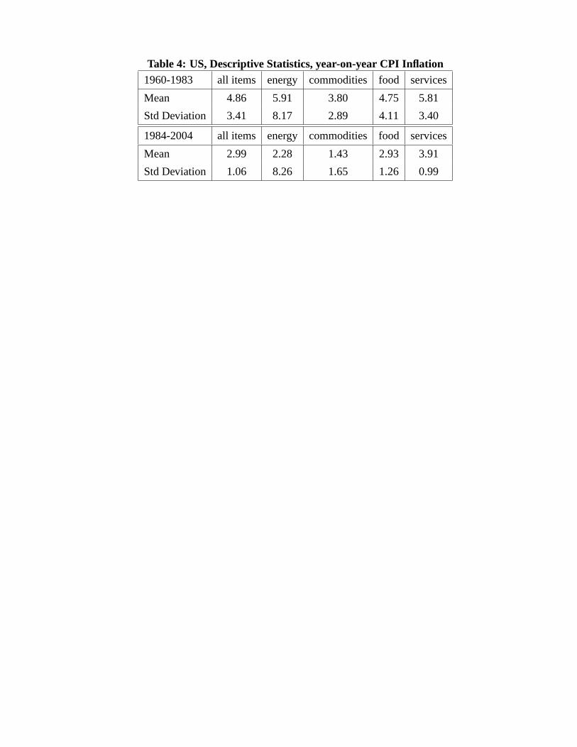
Table 4: US, Descriptive Statistics, year-on-year CPI Inflation1960-1983 all items energy commodities food services
Mean 4.86 5.91 3.80 4.75 5.81
Std Deviation 3.41 8.17 2.89 4.11 3.40
1984-2004 all items energy commodities food services
Mean 2.99 2.28 1.43 2.93 3.91
Std Deviation 1.06 8.26 1.65 1.26 0.99

Table 5: Tests of Equal Forecast Accuracy, US year-on-year inflation1970-1983
method RMSPE (altern)/ t-stat max t-stat. χ2 χ2 Reality
RMSPE (bench) adj. adj. adj unadj check
AR(AIC) (bench) 0.307
Test AR
vs VARa,f(AIC) 1.039 0.666
vs VARa,e(AIC) 1.029 0.891
vs VARa,c(AIC) 1.016 1.743∗
vs VARa,s(AIC) 0.986 2.311∗
vs 4 models 2.311∗ 7.743 7.207 0.032
critical value 1.282 1.902 7.78 7.78 0.118
1984-2004
method RMSPE (altern)/ t-stat max t-stat χ2 χ2 Reality
RMSPE (bench) adj. adj. adj unadj check
AR(AIC) (bench) 0.187
Test AR
vs VARa,f(AIC) 0.999 1.860∗
vs VARa,e(AIC) 1.097 −0.027
vs VARa,c(AIC) 1.048 0.290
vs VARa,s(AIC) 1.027 −0.463
vs 4 models 1.860 3.905 11.926∗ 0.0007
critical value 1.282 1.919 7.78 7.78 0.059
Note: Forecast evaluation for 1 month ahead forecasts; actual RMSPE (non annualised) for
AR(AIC) benchmark model in percentage points, for other models RMSPE relative to AR (RM-
SPE (altern)/RMSPE (bench)); rolling estimation window; rolling estimation samples 1960(1) to
1970(1),...,1983(12) (i.e. R=120 and P=168) and 1960(1) to 1984(1),...,2004(12), (i.e. R=288 and
P=252); maximum number of lags:p = 13; Subscripts indicate model selection procedure, AIC:
Akaike criterion, superscripts indicate model, VARa,f : VAR with lags of aggregate and food infla-
tion, VARa,e: VAR with lags of aggregate and energy inflation, VARa,c: VAR with lags of aggregate
and commodities inflation, VARa,s: VAR with aggregate and services inflation; model specification in
terms of month-on-month inflation; forecast evaluation for year-on-year inflation; estimated correlation
betweenfi = e0 − ei, for comparing model i=1,...,4 to the benchmark;critical value of respective test
statistic (simulated for max t-stat adj.);* indicates significance on a 10% nominal significance level

Table 6: Tests of Equal Forecast Accuracy, US year-on-year inflation1970-1983
method RMSPE (altern)/ t-stat max t-stat χ2 χ2 Reality
RMSPE (bench) adj. adj. adj unadj check
AR(AIC) (bench) 0.307
Test AR
vs VARa,y(AIC) 0.987 2.013∗
vs VARa,u(AIC) 0.974 3.439∗
vs VARa,c(AIC) 1.016 1.743∗
vs VARa,s(AIC) 0.986 2.311∗
vs 4 models 3.439∗ 21.762∗ 2.432 0.061
critical value 1.282 1.917 7.78 7.78 0.146
1984-2004
method RMSPE (altern)/ t-stat max t-stat χ2 χ2 Reality
RMSPE (bench) adj. adj. adj unadj check
AR(AIC) (bench) 0.187
Test AR
vs VARa,y(AIC) 1.046 −0.047
vs VARa,u(AIC) 1.024 1.867∗
vs VARa,c(AIC) 1.048 0.290
vs VARa,s(AIC) 1.027 −0.463
vs 4 models 1.867 4.605 12.680∗ 0.026
critical value 1.282 1.934 7.78 7.78 0.046
Note: Forecast evaluation for 1 month ahead forecasts; actual RMSPE (non annualised) for
AR(AIC) benchmark model in percentage points, for other models RMSPE relative to AR (RM-
SPE (altern)/RMSPE (bench)); rolling estimation window; rolling estimation samples 1960(1) to
1970(1),...,1983(12) (i.e. R=120 and P=168) and 1960(1) to 1984(1),...,2004(12), (i.e. R=288 and
P=252); maximum number of lags:p = 13; Subscripts indicate model selection procedure, AIC: Akaike
criterion, superscripts indicate model, VARa,y: VAR with lags of aggregate inflation and output growth,
VARa,u: VAR with lags of aggregate inflation and change in unemployment, VARa,c: VAR with lags
of aggregate and commodities inflation, VARa,s: VAR with aggregate and services inflation; model
specification in terms of month-on-month inflation; forecast evaluation for year-on-year inflation; esti-
mated correlation betweenfi = e0 − ei, for comparing model i=1,...,4 to the benchmark;critical value
of respective test statistic (simulated for max t-stat adj.);* indicates significance on a 10% nominal
significance level