Embed Size (px)
Citation preview
OCS Study BOEM 2014-607
U.S. Department of the Interior Bureau of Ocean Energy Management
Gulf of Mexico OCS Region
Forcing Functions Governing Salt Transports Processes in Coastal Navigation Canals and Connectivity to Surrounding Wetland Landscapes in South Louisiana Using Houma Navigation Canal as a Surrogate
S
salinity (psu)
OCS Study BOEM 2014-607
Published by U.S. Department of the Interior
Bureau of Ocean Energy Management
Gulf of Mexico OCS Region
New Orleans, LA June 2014
Forcing Functions Governing Salt Transport Processes in Coastal Navigation Canals and Connectivity to Surrounding Wetland Landscapes in South Louisiana Using Houma Navigation Canal as a Surrogate
Authors
Gregg A. Snedden
Prepared under BOEM Contract M10PG00037 by Gregg A. Snedden U.S. Geological Survey Wetlands Research Center Baton Rouge, LA 70803

iii
DISCLAIMER
This report was prepared under contract between the Bureau of Ocean Energy Management
(BOEM) and the U.S. Geological Survey. This report has been technically reviewed by BOEM,
and it has been approved for publication. Approval does not necessarily signify that the contents
reflect the views and policies of BOEM, nor does mention of trade names or commercial
products constitute endorsement or recommendation for use.
REPORT AVAILABILITY
To download a PDF file of this Gulf of Mexico OCS Region report, go to the U.S. Department of
the Interior, Bureau of Ocean Energy Management, Environmental Studies Program Information
System website and search on OCS Study BOEM 2014-607.
This report can be viewed at select Federal Depository Libraries. It can also be obtained from
the National Technical Information Service; the contact information is below.
U.S. Department of Commerce
National Technical Information Service
5301 Shawnee Rd.
Springfield, Virginia 22312
Phone: (703) 605-6000, 1(800)553-6847
Fax: (703) 605-6900
Website: http://www.ntis.gov/
CITATION
Snedden, Gregg A. 2014. Forcing functions governing salt transport processes in coastal
navigation canals and connectivity to surrounding wetland landscapes in South
Louisiana using Houma Navigation Canal as a Surrogate. U.S. Dept. of the Interior,
Bureau of Ocean Energy Management, Gulf of Mexico OCS Region, New Orleans, LA.
OCS Study BOEM 2014-607. 84 pp.
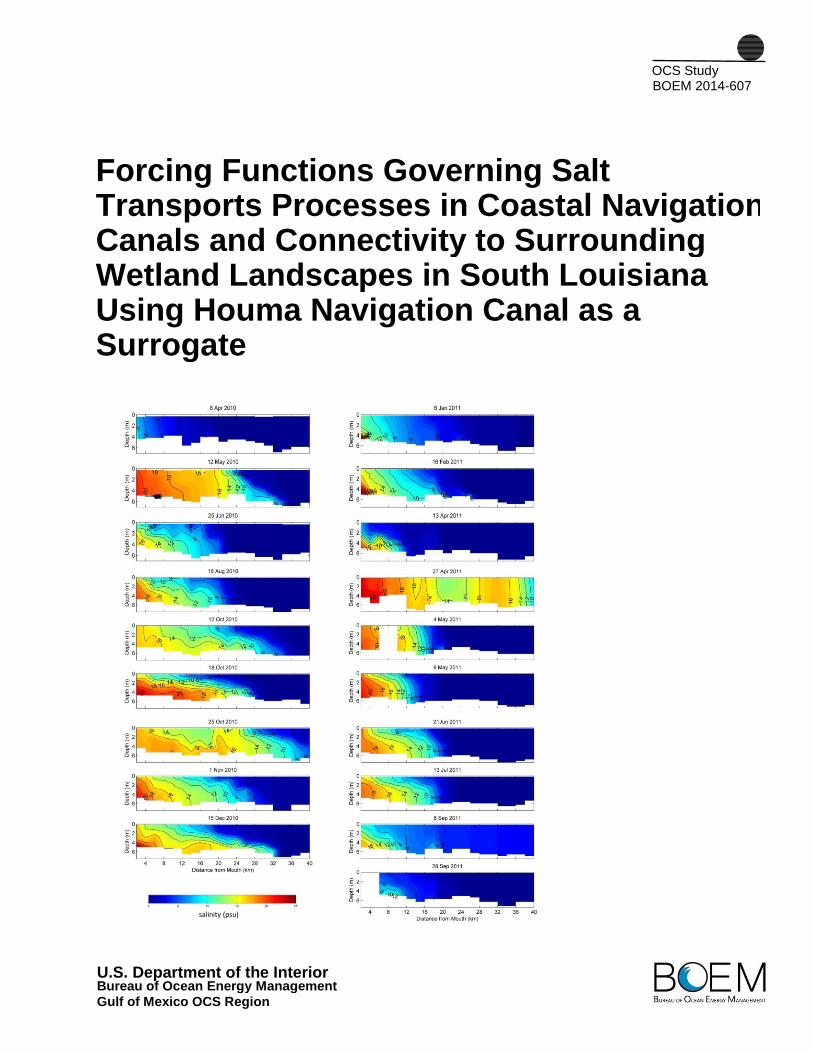
ABOUT THE COVER
Graphic of the longitudinal salinity profiles for the 19 conductivity-temperature depth (CTD)
transects conducted between April 2010 and September 2011.

v
ACKNOWLEDGEMENTS
Funding for this work was provided by the Bureau of Ocean Energy Management (BOEM).
The U.S. Geological Survey Louisiana Water Science Center provided assistance installing,
downloading and servicing field instrumentation and also with data collection during 25-hour
tidal cycle surveys. Harry Bourg Corporation graciously granted permission to collect data on
their property. Erick Swenson and Sarai Piazza provided helpful comments to earlier versions of
this document. Thanks to Arie Kaller for carefully reading all the quarterly reports, keeping
things on track, and providing feedback throughout this project.
This work is dedicated to the memory of Larry Hartzog, the original contract manager for
this study. Larry spent nearly his entire career working to better understand and manage
Louisiana’s aquatic resources. He and his tasty craft beer are dearly missed.


vii
FOREWORD
DEDICATED IN HONOR AND MEMORY OF Larry Hartzog
This dedication reflects memories of the colleagues that worked with Larry Hartzog during
his career. Larry died soon after retiring, approximately two years before this report was
completed for the Bureau of Ocean Energy Management.
_______________________________________
Larry Hartzog is recognized for his work of over three decades
for the Federal Government working and his devotion to nearshore
habitats and species in the Gulf of Mexico especially the Gulf
sturgeon.
I first met Larry Hartzog in June of 1979 when I began work for
the U.S. Army Corps of Engineers, New Orleans District. Larry had
been working there for about a year before I arrived. We had a lot in
common both personally and professionally and we became close
friends. We both had backgrounds in fisheries and had both previously worked for State
agencies involved in fisheries management. Our families also became good friends and my wife
and I asked Larry and his wife Nancy to become our son’s godparents.
Larry and I worked together in the Environmental Quality Section at the New Orleans
District for about ten years. Over that time period, we were fortunate to work with several other
colleagues with similar backgrounds and experience and we formed a close-knit working unit.
Most of our work involved the preparation of environmental impact statements and
environmental assessments for navigation, flood control, hurricane protection, and wetland
restoration projects. These documents were prepared in order to comply with the National
Environmental Policy Act (NEPA). We frequently assisted one another on various projects and
this often included field work. On several occasions I worked in the field with Larry. On one
memorable trip, we spent about a week assessing the standing crops of fish in oxbow lakes along
the Red River in Louisiana. As part of this work, we deployed block nets. These nets
encompass an acre of water. Rotenone is then applied to the area to kill the fish and, over a
period of several days, all of the fish within the netted area are collected, weighed, measured, and
identified. One day, Larry and I went to set one of the block nets. I was driving the boat. I
placed the bow of the boat on the shoreline. Larry jumped off the bow of the boat to begin
attaching one end of the net to the shore. Since the bow of the boat was touching the shore, he
assumed the water was shallow and jumped over into the water. Unfortunately, the bank was a
sheer drop-off and Larry, who was several inches over six-feet tall, completely disappeared
beneath the surface. The first thing I saw was his straw hat floating on the surface, followed
viii
shortly thereafter by Larry surfacing, blowing like a porpoise, and uttering a variety of
expletives. On another occasion, Larry was working on a write-up dealing with the effects of
turbidity on fish. Something came up that required Larry to be out of the office for a week or so
and I was asked to finish up the report. Larry gave me what he had written so far. This was in
the early 1980’s and much of our writing was still done by longhand. Larry’s handwriting was
notoriously bad, rivaling that of any doctor. There were several portions of the report that I
could simply not decipher. I did the best I could and when Larry returned I asked him clarify his
handwriting. With some embarrassment, he acknowledged that he could not read it either and
we both laughed about this.
In January of 1989, I left the U.S. Army Corps of Engineers and went to work for the
Minerals Management Service (MMS), Office of Leasing and Environment, in New Orleans.
Over the years, Larry and I kept in touch and, as fate would have it, in January of 2007, Larry
came to work at MMS in the office of Leasing and Environment as well. During his nearly 30
years of work at the New Orleans District of the Corps, Larry worked on many coastal projects
and dealt with many wetland issues. Due to that knowledge and experience, one of his primary
assignments was to prepare wetland analyses for NEPA documents dealing with the impacts of
oil and gas activities regulated by the Agency. During my tenure at the Corps, I worked on many
wetland projects and over my 20 years at MMS I was involved in many wetland issues. Due to
our common background and close friendship, Larry and I frequently discussed NEPA and
wetland issues. I retired from MMS in January of 2009; however, in October 2010, I returned to
MMS as a reemployed annuitant and once again enjoyed the opportunity to work and socialize
with Larry on a regular basis.
As a scientist, Larry’s professional integrity and attention to detail were exemplary. He shied
from using anecdotal information in his analyses and always strived to use credible, peer-
reviewed information. Over the years, he developed and maintained many professional contacts
in Federal, State, and local agencies as well as academia and coordinated with these individuals
regarding the latest studies and information. In addition to his work related to wetlands, Larry
was also heavily involved with assessing the impacts of Federal activities on several species of
sturgeon.
As a person, Larry was one of the most socially adept people I have ever met. He made
friends easily and enjoyed entertaining both friends and family. His love of cooking, jazz, and
brewing beer were very conducive to these social interactions.
I consider it a great privilege to have the opportunity to honor the career of Larry Hartzog in
association with this study regarding salt transport processes via navigation canals and impacts to
surrounding wetlands.
Dennis L. Chew
Chief, Environmental Assessment Section (Retired)
Gulf of Mexico OCS Region
_______________________________________
ix
Larry Hartzog and I both came to the New Orleans District, Corps of Engineers in 1978.
Both of us came from the Florida Game and Freshwater Fish Commission; he as a fish biologist
working up around the Saint Johns River, and me as a fish biologist in central Florida (Kissimee
River, etc). We did not know each other well while in Florida, but we sure knew a lot of people
in common and could both tell whopper stories. I guess we both continued our growing up
together (we were born within a few months of each other) and did some of the earlier NEPA
work for the Corps. After a while we understood that NEPA was basically a four letter word-
and only to be said when absolutely necessary. We worked together in New Orleans till I left for
Washington DC in 1990. Although Larry took his work seriously he never let his tasks interfere
with his relationships. In fact, during my entire working career, and before and since, I have
never met more relational person than Larry Hartzog. Many was the time I could be a little
down and then totally revived after just a few moments of conversation and laughter in his
cubicle. I saw the same magic occur with many other defeated and downtrodden biologists.
Larry had a magical personality and I will always miss him.
Dave Reece
U.S. Army Corps of Engineers (Retired)
______________________________________
I met Larry in 1992 when I began an internship at the U.S Army Corp of Engineers. For
several years we spoke on occasions regarding our shared hobby of brewing beer. It wasn’t until
I transferred to the Environmental Branch in 2001 that I became close friends with Larry. Not
only was he a close friend but a mentor as well. He was never too busy to provide guidance or
answer questions. Shortly after Hurricane Katrina devastated New Orleans, Larry and I worked
on Task Force Guardian, providing environmental support to engineering teams tasked with
rebuilding the levees surrounding New Orleans to pre-Katrina elevations. Because the Corps
was tasked with the rebuilding effort in less than a year, we worked many long days together
both in the field and the office. Despite the stress, conflicts, and long hours; Larry never slowed
nor let it affect him. Whenever the stress built up I would stop by his desk or take a trip with
him in the field and he would always seem to make things better. I believe that he was the one
factor that helped me and our other team members keep our sanity during those trying times. I
am proud of the work we performed together on such a successful operation. On the same day in
x
2007, Larry and I both transferred to Minerals Management Service and worked together for
several years until his retirement in early 2012. His death occurred about three weeks following
his retirement.
Larry and I went to many beer festivals together along with our homebrew club and he was
well known throughout the Gulf coast brewing communities. An annual beer festival that our
homebrew club organizes has been named in his honor and is a well-attended event not only by
fellow home brewers but also many friends and colleagues attend as well. Larry was also a lover
of jazz. He would share his love of music to anyone willing to listen and loved attending the
annual New Orleans Jazz festival. He loved bringing people along to the festival to open new
ears to jazz and other forms of music. Larry is sorely missed. Anyone who never met or knew
Larry Hartzog has been cheated for he was such a good person and a joy to spend time with.
Casey Rowe
Environmental Operations Section
Gulf of Mexico OCS Region
______________________________________
I worked with Larry and had the cubicle next to him or across from him for the entire 15
years I worked at the U.S Army Corp of Engineers. He was a great storyteller and a fun person
that helped the day go by faster. When he would get typing on his computer he would start
humming and making noises, throwing in a “Yeehaa” for good measure every now and then. I
miss him, as he was a good friend.
Bruce Baird
Biological Sciences Section
Bureau of Ocean Energy Management
xi
ABSTRACT
Understanding how circulation and mixing processes in coastal navigation canals
influence the exchange of salt between marshes and coastal ocean, and how those processes
are modulated by external physical processes, is critical to anticipating effects of future
actions and circumstance. Examples of such circumstances include deepening the channel,
placement of locks in the channel, changes in freshwater discharge down the channel,
changes in outer continental shelf (OCS) vessel traffic volume, and sea level rise. The study
builds on previous BOEM-funded studies by investigating salt flux variability through the
Houma Navigation Canal (HNC). It examines how external physical factors, such as
buoyancy forcing and mixing from tidal stirring and OCS vessel wakes, influence dispersive
and advective fluxes through the HNC and the impact of this salt flux on salinity in nearby
marshes.
This study quantifies salt transport processes and salinity variability in the HNC and
surrounding Terrebonne marshes. Data collected for this study include time-series data of
salinity and velocity in the HNC, monthly salinity-depth profiles along the length of the
channel, hourly vertical profiles of velocity and salinity over multiple tidal cycles, and
salinity time series data at three locations in the surrounding marshes along a transect of
increasing distance from the HNC.
Two modes of vertical current structure were identified. The first mode, making up 90%
of the total flow field variability, strongly resembled a barotropic current structure and was
coherent with alongshelf wind stress over the coastal Gulf of Mexico. The second mode was
indicative of gravitational circulation and was linked to variability in tidal stirring and the
longitudinal salinity gradients along the channel’s length. Diffusive process were dominant
drivers of upestuary salt transport, except during periods of minimal tidal stirring when
gravitational circulation became more important. Salinity in the surrounding marshes was
much more responsive to salinity variations in the HNC than it was to variations in the
lower Terrebonne marshes, suggesting that the HNC is the primary conduit for saltwater
intrusion to the middle Terrebonne marshes. Finally, salt transport to the middle Terrebonne
marshes directly associated with vessel wakes was negligible.

xiii
CONTENTS
ACKNOWLEDGEMENTS .......................................................................................................................... v
FOREWORD .............................................................................................................................................. vii
ABSTRACT ................................................................................................................................................. xi
LIST OF FIGURES .................................................................................................................................... xv
LIST OF TABLES ..................................................................................................................................... xxi
1. INTRODUCTION .................................................................................................................................. 1
2. METHODS ............................................................................................................................................. 7
2.1. Data Collection ........................................................................................................................... 7
2.2. Data Analysis .............................................................................................................................. 9
3. RESULTS AND DISCUSSION ........................................................................................................... 11
3.1. Tidal Variability ........................................................................................................................ 11
3.2. Subtidal Current Variability ...................................................................................................... 13
3.3 Vertical Variation in Subtidal Velocity Structure at HNC1 and HNC3 ................................... 15
3.4 Salinity Stratification at HNC2 ................................................................................................. 26
3.5 Salinity Transects and Saltwater Intrusion Length ................................................................... 29
3.6 Synoptic Salinity and Velocity Surveys Over Tidal Cycles ..................................................... 32
3.7 Salt Transport from the HNC to the Surrounding Marsh Landscape ........................................ 42
3.8 Influence of Vessel Wakes on Salt Flux from the HNC into Marshes ..................................... 46
4. CONCLUSIONS................................................................................................................................... 49
LITERATURE CITED ............................................................................................................................... 53
APPENDIX ................................................................................................................................................. 59

xv
LIST OF FIGURES
Figure 1. Coastal Louisiana showing the Mississippi River, Atchafalaya River, Gulf
Intracoastal Waterway, and Houma Navigation Canal (waterway in the
inset). Inset is enlarged in Figure 2. ..................................................................... 3
Figure 2. Location of stations on CTD transect (red dots), time series salinity and
velocity stations (yellow squares; HNC1, HNC2, HNC3), marsh salinity
stations (green circles; M1, M2, M3, CRMS0307), and vessel wake study
location (white star; Four Point Bayou). Synoptic sampling of salinity
and current velocity vertical profiles was conducted at HNC2 and HNC3. ........ 4
Figure 3. Inventory of salinity time series (red lines), velocity time series (blue lines),
salinity transects (blue dots), tidal cycle measurements at HNC2 and
HNC3 (red dots) and ancillary data (wind stress, Atchafalaya River
discharge; black lines) used in this study. ........................................................... 7
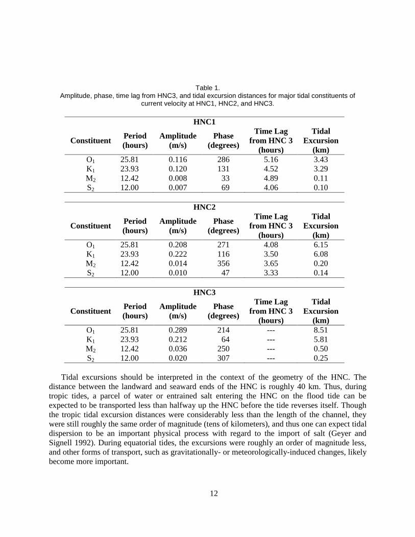
Figure 4. Mean subtidal water column velocity at HNC1 (top), HNC2 (middle),
HNC3 (first time series, bottom), and HNC3a (second time series,
bottom). .............................................................................................................. 13
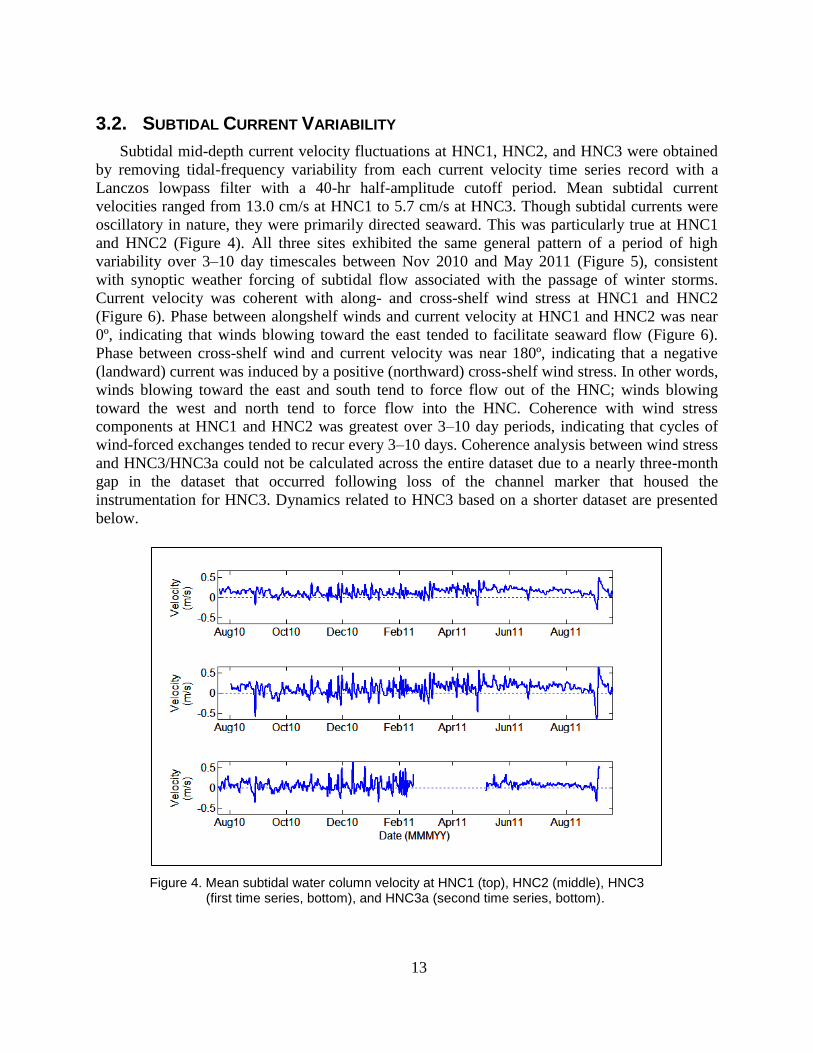
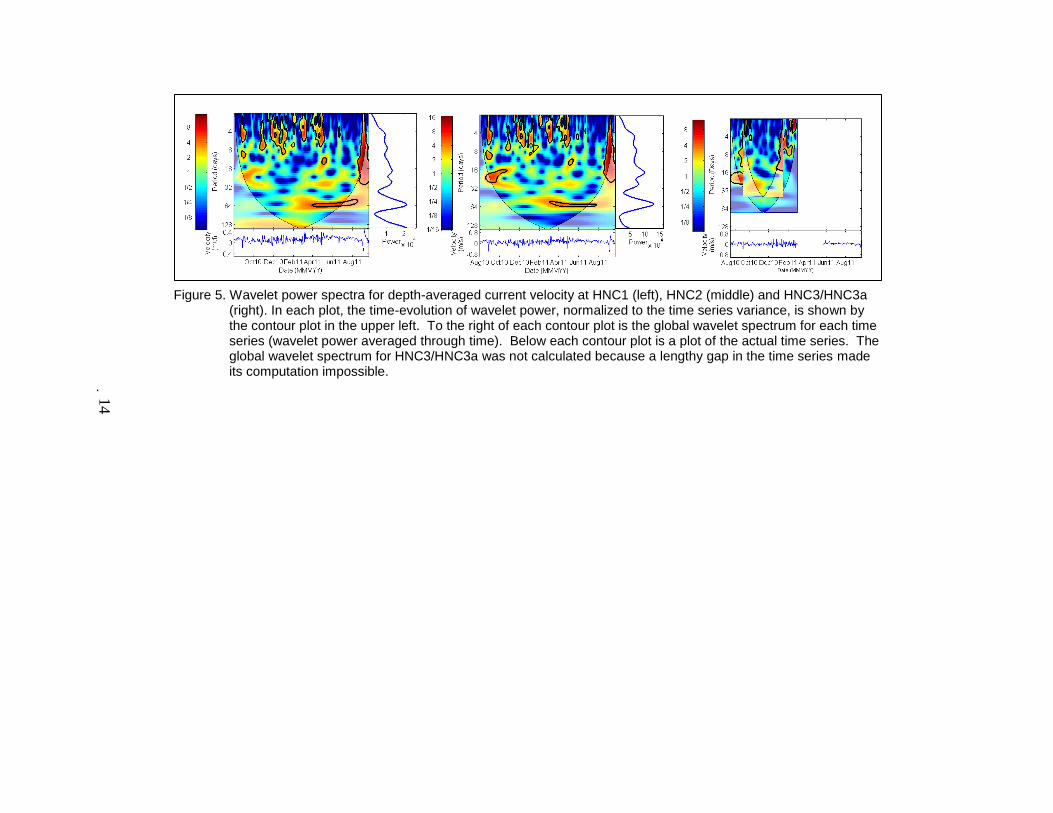
Figure 5. Wavelet power spectra for depth-averaged current velocity at HNC1 (left),
HNC2 (middle) and HNC3/HNC3a (right). In each plot, the time-
evolution of wavelet power, normalized to the time series variance, is
shown by the contour plot in the upper left. To the right of each contour
plot is the global wavelet spectrum for each time series (wavelet power
averaged through time). Below each contour plot is a plot of the actual
time series. The global wavelet spectrum for HNC3/HNC3a was not
calculated because a lengthy gap in the time series made its computation
impossible. ......................................................................................................... 14
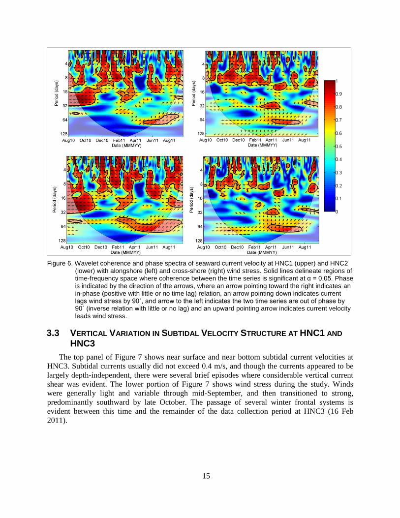
Figure 6. Wavelet coherence and phase spectra of seaward current velocity at HNC1
(upper) and HNC2 (lower) with alongshore (left) and cross-shore (right)
wind stress. Solid lines delineate regions of time-frequency space where
coherence between the time series is significant at α = 0.05. Phase is
indicated by the direction of the arrows, where an arrow pointing toward
the right indicates an in-phase (positive with little or no time lag)
relation, an arrow pointing down indicates current lags wind stress by
90˚, and arrow to the left indicates the two time series are out of phase by
90˚ (inverse relation with little or no lag) and an upward pointing arrow
indicates current velocity leads wind stress. ...................................................... 15
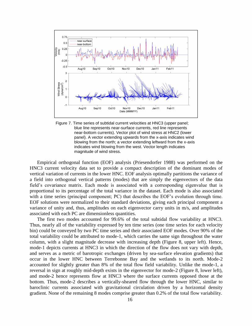
Figure 7. Time series of subtidal current velocities at HNC3 (upper panel; blue line
represents near-surface currents, red line represents near-bottom
currents). Vector plot of wind stress at HNC2 (lower panel). A vector
extending upwards from the x-axis indicates wind blowing from the
north; a vector extending leftward from the x-axis indicates wind
blowing from the west. Vector length indicates magnitude of wind stress. ...... 16
xvi
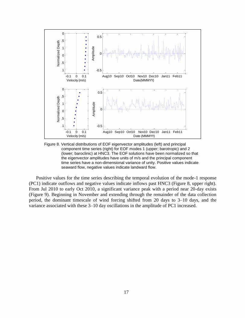
Figure 8. Vertical distributions of EOF eigenvector amplitudes (left) and principal
component time series (right) for EOF modes 1 (upper; barotropic) and 2
(lower; baroclinic) at HNC3. The EOF solutions have been normalized
so that the eigenvector amplitudes have units of m/s and the principal
component time series have a non-dimensional variance of unity.
Positive values indicate seaward flow, negative values indicate landward
flow. ................................................................................................................... 17
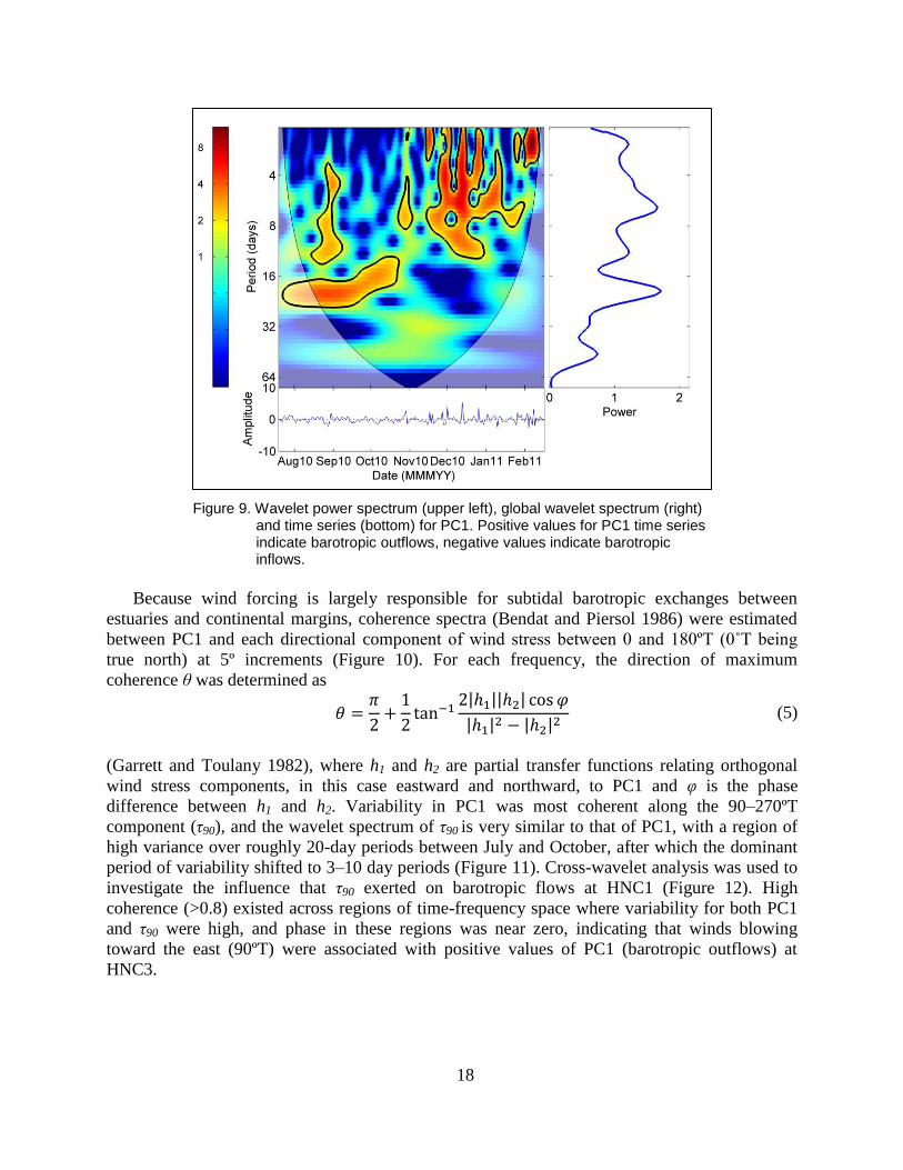
Figure 9. Wavelet power spectrum (upper left), global wavelet spectrum (right) and
time series (bottom) for PC1. Positive values for PC1 time series indicate
barotropic outflows, negative values indicate barotropic inflows. .................... 18
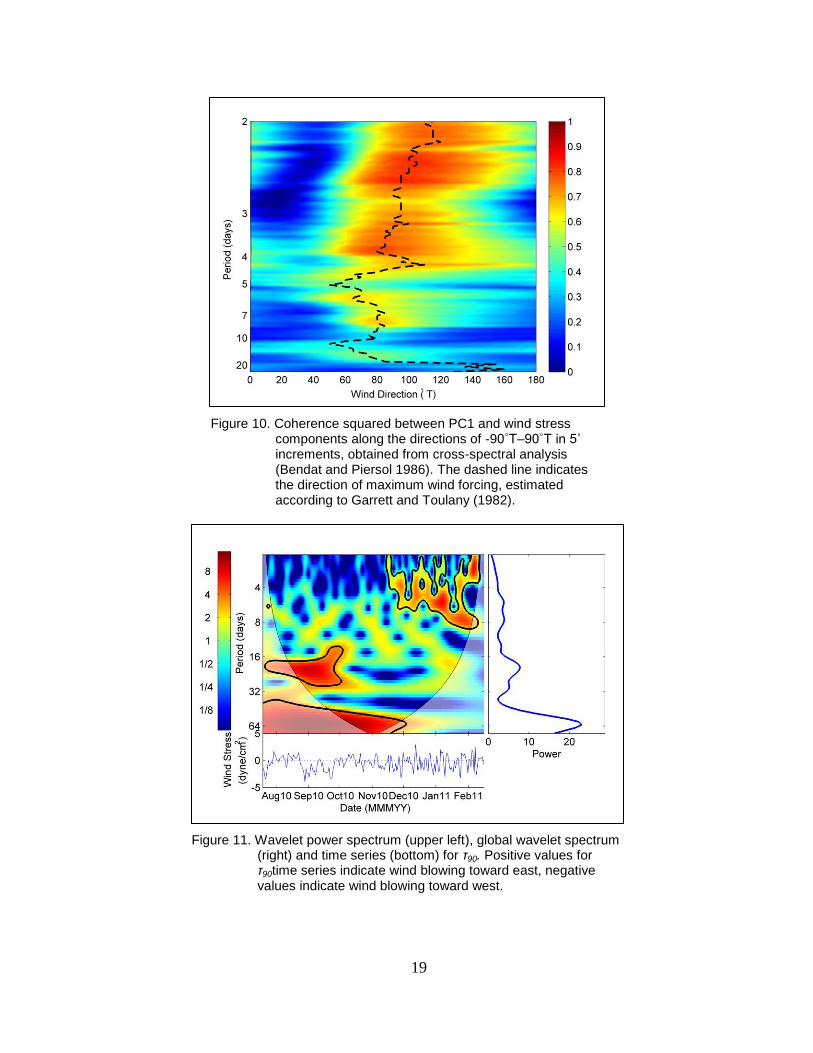
Figure 10. Coherence squared between PC1 and wind stress components along the
directions of -90˚T–90˚T in 5˚ increments, obtained from cross-spectral
analysis (Bendat and Piersol 1986). The dashed line indicates the
direction of maximum wind forcing, estimated according to Garrett and
Toulany (1982). ................................................................................................. 19
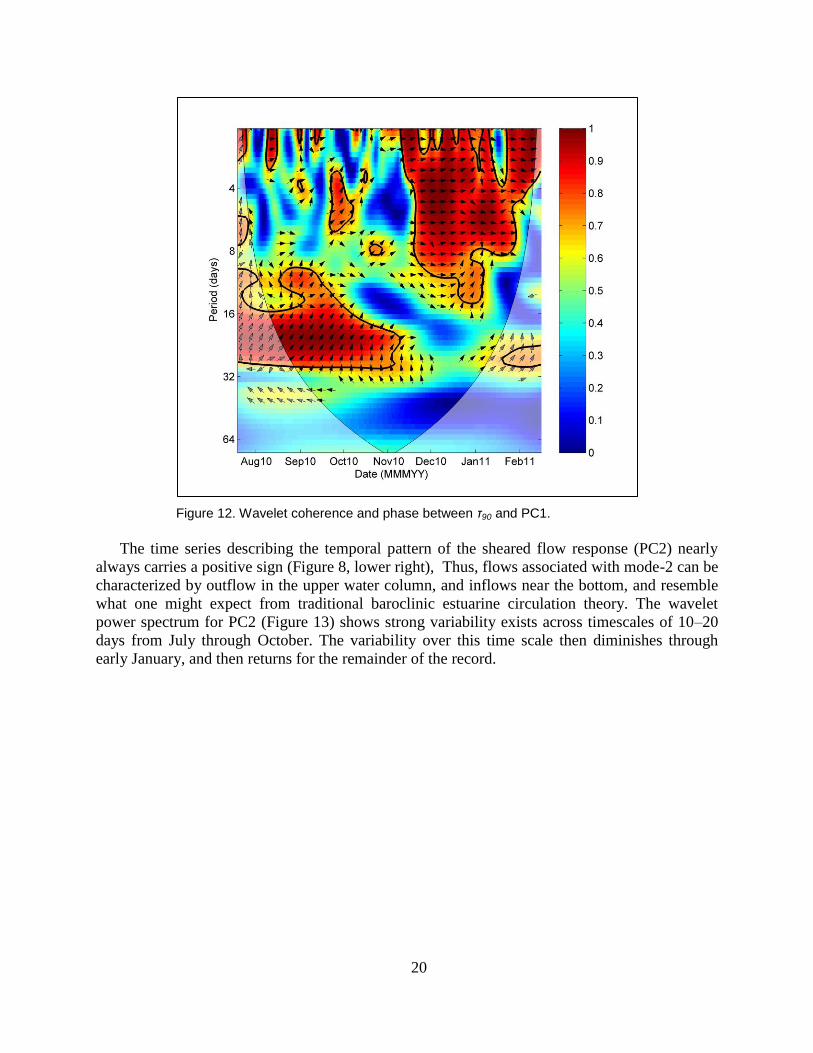
Figure 11. Wavelet power spectrum (upper left), global wavelet spectrum (right) and
time series (bottom) for τ90. Positive values for τ90time series indicate
wind blowing toward east, negative values indicate wind blowing toward
west. ................................................................................................................... 19
Figure 12. Wavelet coherence and phase between τ90 and PC1. ............................................ 20
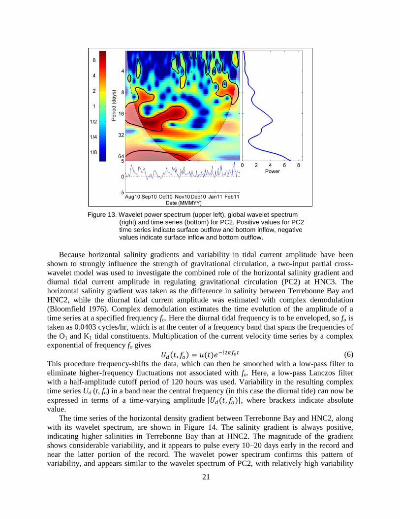
Figure 13. Wavelet power spectrum (upper left), global wavelet spectrum (right) and
time series (bottom) for PC2. Positive values for PC2 time series indicate
surface outflow and bottom inflow, negative values indicate surface
inflow and bottom outflow. ............................................................................... 21
Figure 14. Wavelet power spectrum (upper left), global wavelet spectrum (right) and
time series (bottom) for horizontal density gradient at HNC3, defined as
the difference between salinity at Terrebonne Bay and salinity at HNC2.
Positive values for density gradient time series indicate salinity at
Terrebonne Bay exceeds that at HNC2.............................................................. 22
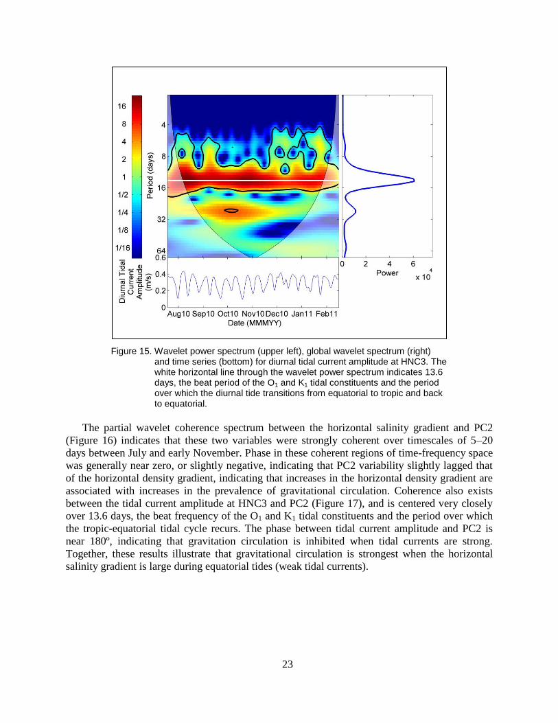
Figure 15. Wavelet power spectrum (upper left), global wavelet spectrum (right) and
time series (bottom) for diurnal tidal current amplitude at HNC3. The
white horizontal line through the wavelet power spectrum indicates 13.6
days, the beat period of the O1 and K1 tidal constituents and the period
over which the diurnal tide transitions from equatorial to tropic and back
to equatorial. ...................................................................................................... 23
Figure 16. Wavelet coherence and phase between the horizontal salinity gradient and
PC2 at HNC3. .................................................................................................... 24
Figure 17. Wavelet coherence and phase between the diurnal tidal current amplitude
and PC2 at HNC3. ............................................................................................. 24
Figure 18. Vertical distributions of EOF eigenvector amplitudes (left) and principal
component time series (right) for EOF modes 1 (upper; barotropic) and 2
xvii
(lower; baroclinic) at HNC1. The EOF solutions have been normalized
so that the eigenvector amplitudes have units of m s-1
and the principal
component time series have a non-dimensional variance of unity.
Positive values indicate seaward flow, negative values indicate landward
flow. ................................................................................................................... 25
Figure 19. Tidal height, current velocity, and stratification at HNC2, 2 Aug– 6 Aug
2010. .................................................................................................................. 26
Figure 20. Tidally-averaged vertical salinity stratification at HNC2 (top), diurnal tidal
current amplitude at HNC2 (middle), and Atchafalaya River discharge at
Morgan City, LA (bottom). ............................................................................... 27
Figure 21. Wavelet power spectrum (upper left), global wavelet spectrum (right) and
time series (bottom) for tidally-averaged salinity stratification at HNC2.
The white horizontal line through the wavelet power spectrum indicates
13.6 days, the beat period of the O1 and K1 tidal constituents and the
period over which the diurnal tide transitions from equatorial to tropic
and back to equatorial. ....................................................................................... 28
Figure 22. Wavelet coherence and phase between the diurnal tidal current amplitude
and tidally-averaged salinity stratification at HNC2. The white horizontal
line through the wavelet coherence spectrum indicates 13.6 days, the beat
period of the O1 and K1 tidal constituents and the period over which the
diurnal tide transitions from equatorial to tropic and back to equatorial. .......... 28
Figure 23. Longitudinal salinity profiles for the 19 conductivity-temperature depth
(CTD) transects conducted between Apr 2010 and Sep 2011. Letters
above plots correspond to sampling dates indicated by dotted lines in
Figure 24. ........................................................................................................... 30
Figure 24. Atchafalaya River discharge (upper panel) and diurnal tidal amplitude
conditions (lower panel) for each of the 19 CTD transects conducted
between Apr 2010 and Sep 2011. Letters and dashed vertical lines
correspond to contour plots in Figure 23. .......................................................... 31
Figure 25. Multiple regression surface (F = 29.3, p<0.0001, r2 = 0.83) obtained using
eastward wind stress (τ90) and Atchafalaya River discharge (q) as
predictors for saltwater intrusion length in the Houma Navigation Canal.
Blue circles indicate individual data points, sticks extend from regression
surface to data points to indicate residual error. ................................................ 32
Figure 26. Salinity (PSU; top) and velocity (m/s; bottom) profiles at HNC2 from 26-
hour synoptic surveys during tropic (13-14 Oct 2010; left) and equatorial
(19-20 Oct 2010; right) tidal conditions during low Atchafalaya River
discharge (October). Vertical axis represents depth; horizontal axis
represents time. Positive values for velocity indicate ebb currents;
negative velocity values indicate flood currents ................................................ 35
Figure 27. Salinity (PSU; top) and velocity (m/s; bottom) profiles at HNC3 from 26-
hour synoptic surveys during tropic (13-14 Oct 2010; left) and equatorial
xviii
(19-20 Oct 2010; right) tidal conditions during low Atchafalaya River
discharge (October). Vertical axis represents depth; horizontal axis
represents time. Positive values for velocity indicate ebb currents;
negative velocity values indicate flood currents. ............................................... 36
Figure 28. Layer Richardson numbers (RiL) during each of the tidal cycle synoptic
surveys at HNC2 and HNC3. The dotted lines (RiL equal 2 and 20)
indicate the upper limit for complete mixing and lower limit for full
stratification, respectively. Between these limits water column stability is
transitional. ........................................................................................................ 37
Figure 29. Salinity (PSU; top) and velocity (m/s; bottom) profiles at HNC2 from 26-
hour synoptic surveys during tropic (5-6 May 2011; left) and equatorial
(28-29 Apr 2011; right) tidal conditions during High Atchafalaya River
discharge (April-May). Vertical axis represents depth; horizontal axis
represents time. Positive values for velocity indicate ebb currents;
negative velocity values indicate flood currents. ............................................... 38
Figure 30. Salinity (PSU; top) and velocity (m/s; bottom) profiles at HNC3 from 26-
hour synoptic surveys during tropic (5-6 May 2011; left) and equatorial
(28-29 Apr 2011; right) tidal conditions during High Atchafalaya River
discharge (April-May). Vertical axis represents depth; horizontal axis
represents time. Positive values for velocity indicate ebb currents;
negative velocity values indicate flood currents. ............................................... 39
Figure 31. Classification the HNC according to a stratification-circulation diagram
(Hansen and Rattray 1966) applied to HNC2 (top) and HNC3 (bottom)
during fall (low river flow; left) and spring (high river flow; right) during
tropic (blue) and equatorial (red) tidal conditions. Type 1 estuaries are
well-mixed; type II estuaries are partially mixed. ............................................. 40
Figure 32. Salinity at M1 (top panel), M2 (middle panel), and M3 (bottom panel)
marsh stations. Refer to Figure 2 for station locations. ..................................... 42
Figure 33. Wavelet power spectrum (upper left), global wavelet spectrum (right) and
time series (bottom) for salinity at M1. ............................................................. 43
Figure 34. Wavelet power spectrum (upper left), global wavelet spectrum (right) and
time series (bottom) for salinity at M2. ............................................................. 43
Figure 35. Wavelet power spectrum (upper left), global wavelet spectrum (right) and
time series (bottom) for salinity at M3. ............................................................. 44
Figure 36. Wavelet coherence and phase spectrum between salinity at stations M1
and M2. .............................................................................................................. 45
Figure 37. Partial coherence and phase spectra of salinity at M1 with salinity at M3
(left) and salinity at CRMS0307 with salinity at M3 (right). ............................ 46
Figure 38. Salinity (a), velocity (b), salt flux (c) and cumulative salt flux (d) during
the vessel wake experiment at Four Point Bayou. Positive velocity and
flux indicate water and salt transport from the HNC into the marsh,
xix
negative velocity and flux indicate transport from the marsh into the
HNC. Dashed vertical lines indicate passage of personal water craft in
Four Point Bayou (black indicates passage heading toward HNC; red
indicates passage coming from HNC); solid vertical lines indicate
passage of large vessels in HNC (black indicates passage heading south;
red indicates passage heading north). ................................................................ 47
Figure 39. Depth-specific current velocity associated with gravitational circulation as
predicted by Officer (1976; Equation 18) during tropic (left) and
equatorial (right) tidal conditions under low river flow. Current channel
configuration (H = 4.5 m) shown by blue line, deepened configuration
(H = 6.1 m) shown by red line. Positive values indicate ebb-directed
currents. ............................................................................................................. 51
Figure A1. (top) Time series of periodic signal with constant amplitude (stationary)
and period of one day (left), and wavelet transform of this stationary
signal (right). (bottom) Time series of periodic signal with time-varying
amplitude (nonstationary) and period of one day (left), and wavelet
transform of this nonstationary signal (right). ................................................... 61
Figure A2. (a) Example signal containing multiple, nonstationary, quasi-periodic
component signals such as (b)a diurnal tide, (c) meteorologically-forced
tides, (d) fluvial runoff pulses, (e) a seasonal component, and (f) random
noise. The signal in (a) is simply the sum of signals depicted in (b)-(f). .......... 62
Figure A3. Wavelet power spectrum (upper left), global wavelet spectrum (right) and
time series (bottom) for the example signal in Figure A1(a). Variance of
each component signal, and the time-evolution of that variance, is
captured in the wavelet power spectrum, and variance peaks for each
component signal are evident in the global wavelet spectrum. ......................... 64

xxi
LIST OF TABLES
Table 1. Amplitude, phase, time lag from HNC3, and tidal excursion distances for
major tidal constituents of current velocity at HNC1, HNC2, and HNC3. ....... 12
Table 2. Salt transport terms (kg/m/s) calculated during tidal cycle sampling at
HNC2 and HNC3 under tropic and equatorial tides during low and high
river flow conditions.. ........................................................................................ 41

1
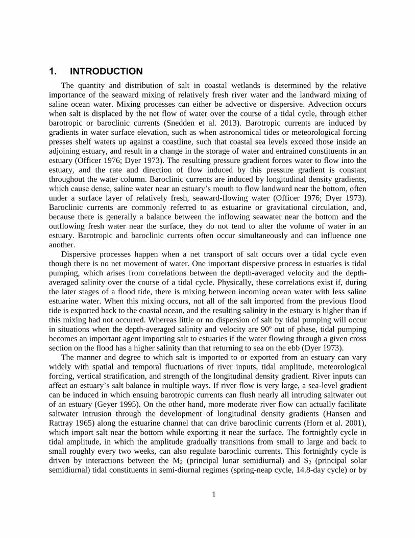
1. INTRODUCTION
The quantity and distribution of salt in coastal wetlands is determined by the relative
importance of the seaward mixing of relatively fresh river water and the landward mixing of
saline ocean water. Mixing processes can either be advective or dispersive. Advection occurs
when salt is displaced by the net flow of water over the course of a tidal cycle, through either
barotropic or baroclinic currents (Snedden et al. 2013). Barotropic currents are induced by
gradients in water surface elevation, such as when astronomical tides or meteorological forcing
presses shelf waters up against a coastline, such that coastal sea levels exceed those inside an
adjoining estuary, and result in a change in the storage of water and entrained constituents in an
estuary (Officer 1976; Dyer 1973). The resulting pressure gradient forces water to flow into the
estuary, and the rate and direction of flow induced by this pressure gradient is constant
throughout the water column. Baroclinic currents are induced by longitudinal density gradients,
which cause dense, saline water near an estuary’s mouth to flow landward near the bottom, often
under a surface layer of relatively fresh, seaward-flowing water (Officer 1976; Dyer 1973).
Baroclinic currents are commonly referred to as estuarine or gravitational circulation, and,
because there is generally a balance between the inflowing seawater near the bottom and the
outflowing fresh water near the surface, they do not tend to alter the volume of water in an
estuary. Barotropic and baroclinic currents often occur simultaneously and can influence one
another.
Dispersive processes happen when a net transport of salt occurs over a tidal cycle even
though there is no net movement of water. One important dispersive process in estuaries is tidal
pumping, which arises from correlations between the depth-averaged velocity and the depth-
averaged salinity over the course of a tidal cycle. Physically, these correlations exist if, during
the later stages of a flood tide, there is mixing between incoming ocean water with less saline
estuarine water. When this mixing occurs, not all of the salt imported from the previous flood
tide is exported back to the coastal ocean, and the resulting salinity in the estuary is higher than if
this mixing had not occurred. Whereas little or no dispersion of salt by tidal pumping will occur
in situations when the depth-averaged salinity and velocity are 90º out of phase, tidal pumping
becomes an important agent importing salt to estuaries if the water flowing through a given cross
section on the flood has a higher salinity than that returning to sea on the ebb (Dyer 1973).
The manner and degree to which salt is imported to or exported from an estuary can vary
widely with spatial and temporal fluctuations of river inputs, tidal amplitude, meteorological
forcing, vertical stratification, and strength of the longitudinal density gradient. River inputs can
affect an estuary’s salt balance in multiple ways. If river flow is very large, a sea-level gradient
can be induced in which ensuing barotropic currents can flush nearly all intruding saltwater out
of an estuary (Geyer 1995). On the other hand, more moderate river flow can actually facilitate
saltwater intrusion through the development of longitudinal density gradients (Hansen and
Rattray 1965) along the estuarine channel that can drive baroclinic currents (Horn et al. 2001),
which import salt near the bottom while exporting it near the surface. The fortnightly cycle in
tidal amplitude, in which the amplitude gradually transitions from small to large and back to
small roughly every two weeks, can also regulate baroclinic currents. This fortnightly cycle is
driven by interactions between the M2 (principal lunar semidiurnal) and S2 (principal solar
semidiurnal) tidal constituents in semi-diurnal regimes (spring-neap cycle, 14.8-day cycle) or by
2
interactions between the O1 (principal lunar diurnal) and K1 (luni-solar diurnal) constituents in
diurnal regimes (tropic-equatorial cycle, 13.6-day cycle). Baroclinic currents that become
established during periods of low tidal amplitude (neap or equatorial tides) are diminished or
eliminated when tidal amplitude becomes large (spring or tropic tides) as turbulence generated at
the channel bottom increases and propagates further up into the overlying water column,
homogenizing the velocity field and reducing the bi-directional flow (Griffin and Leblonde
1990).
Barotropic exchanges of water and salt between estuaries and shelf waters are strongly
influenced by meteorological events (wind forcing), and these exchanges can propagate far into
estuaries and have profound influences on estuarine salinities and water levels. Due to the earth’s
rotation, winds blowing over the coastal ocean transport water to the right of the wind’s direction
in the northern hemisphere (Pond and Pickard 1983). In the case of alongshore winds blowing
parallel to the regional coastline over shelf waters immediately outside of an estuary, these winds
will either cause water to accumulate along a coastal boundary or push water away from it,
depending on which direction they are blowing. The former will result in an influx of saline
ocean water into estuaries, the latter will result in export of estuarine water into the ocean (Wong
and Garvine 1984).
A clear understanding of these processes and how they affect the quantity and distribution of
salt in estuaries of Louisiana is critical, because saltwater intrusion is widely accepted as a
significant contributor to the high rate at which these ecologically and economically important
landscapes have eroded and transitioned to open water. It is widely held that the construction of
straight, deep canals that connect shelf waters to interior marshes has greatly contributed to this
saltwater intrusion over the past several decades (Turner 1997). Since the mid-1800s, ten federal
navigation canals have been constructed in the Louisiana coast, primarily to facilitate
transportation associated with oil and gas exploration and extraction activities.
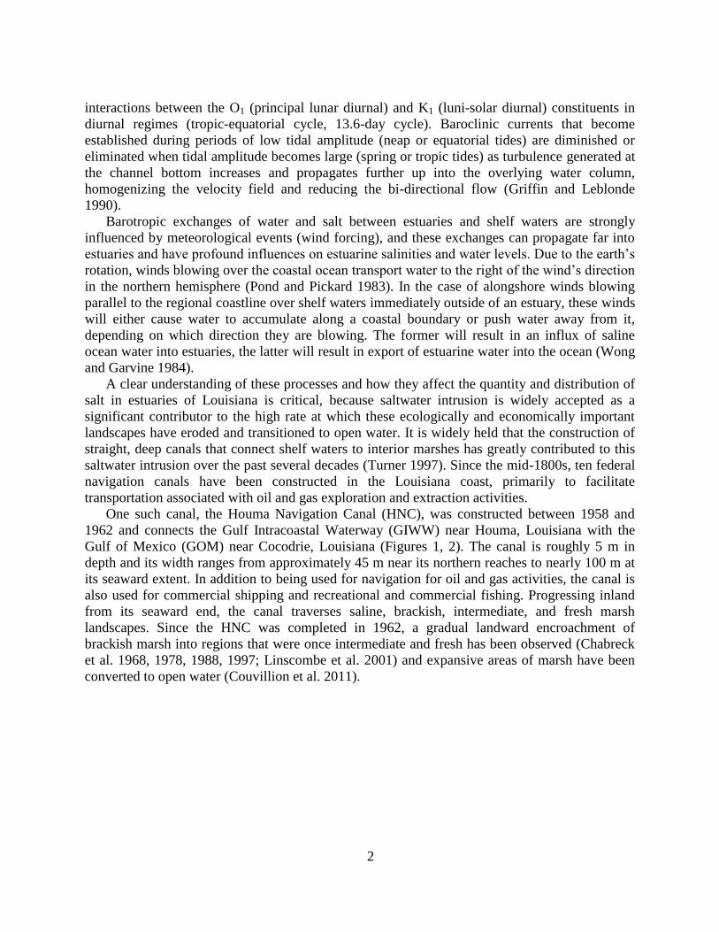
One such canal, the Houma Navigation Canal (HNC), was constructed between 1958 and
1962 and connects the Gulf Intracoastal Waterway (GIWW) near Houma, Louisiana with the
Gulf of Mexico (GOM) near Cocodrie, Louisiana (Figures 1, 2). The canal is roughly 5 m in
depth and its width ranges from approximately 45 m near its northern reaches to nearly 100 m at
its seaward extent. In addition to being used for navigation for oil and gas activities, the canal is
also used for commercial shipping and recreational and commercial fishing. Progressing inland
from its seaward end, the canal traverses saline, brackish, intermediate, and fresh marsh
landscapes. Since the HNC was completed in 1962, a gradual landward encroachment of
brackish marsh into regions that were once intermediate and fresh has been observed (Chabreck
et al. 1968, 1978, 1988, 1997; Linscombe et al. 2001) and expansive areas of marsh have been
converted to open water (Couvillion et al. 2011).
3
Figure 1. Coastal Louisiana showing the Mississippi River, Atchafalaya River, Gulf Intracoastal Waterway, and Houma Navigation Canal (waterway in the inset). Inset is enlarged in Figure 2.
Freshwater inputs to the HNC are strongly associated with discharge of the lower
Atchafalaya River. When discharge is high, a hydraulic gradient is set up in which river water is
conveyed east and west along the Louisiana coast through the GIWW (Figures 1 and 2), which
intersects the Atchafalaya River roughly 20 km upstream from the river’s mouth. Swarzenski
(2003) showed that mean discharge in the GIWW immediately west of its confluence with the
HNC was roughly 90 m3/s less than it was east of the confluence, suggesting that the HNC was
capturing some of the flow and conveying it toward Terrebonne Bay. These river inputs are
typically highest during spring and early summer. In 2011 one of the largest flow events on
record occurred on the Mississippi-Atchafalaya River system, during which the combined flow
of the rivers exceeded project flood capacity (approximately 30,000 m3/s) for six weeks between
May and June.
4
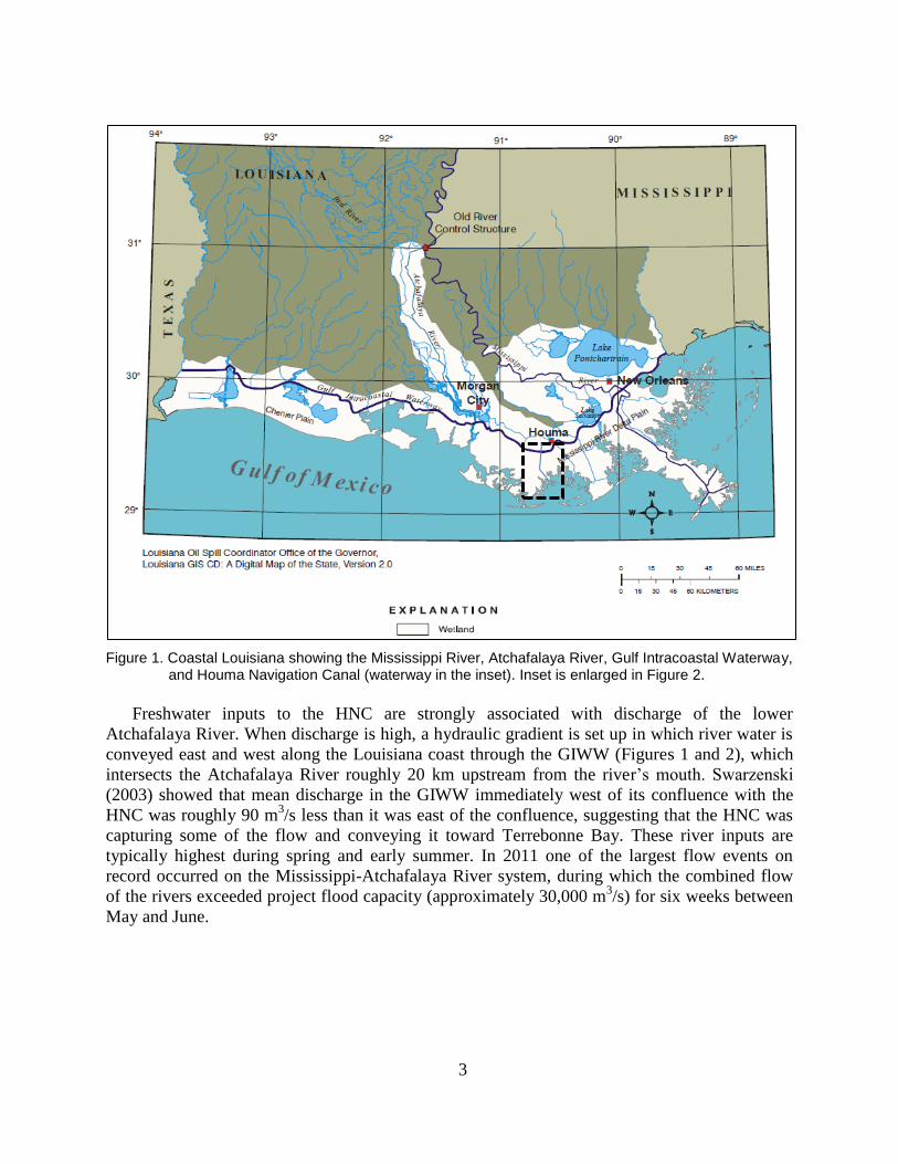
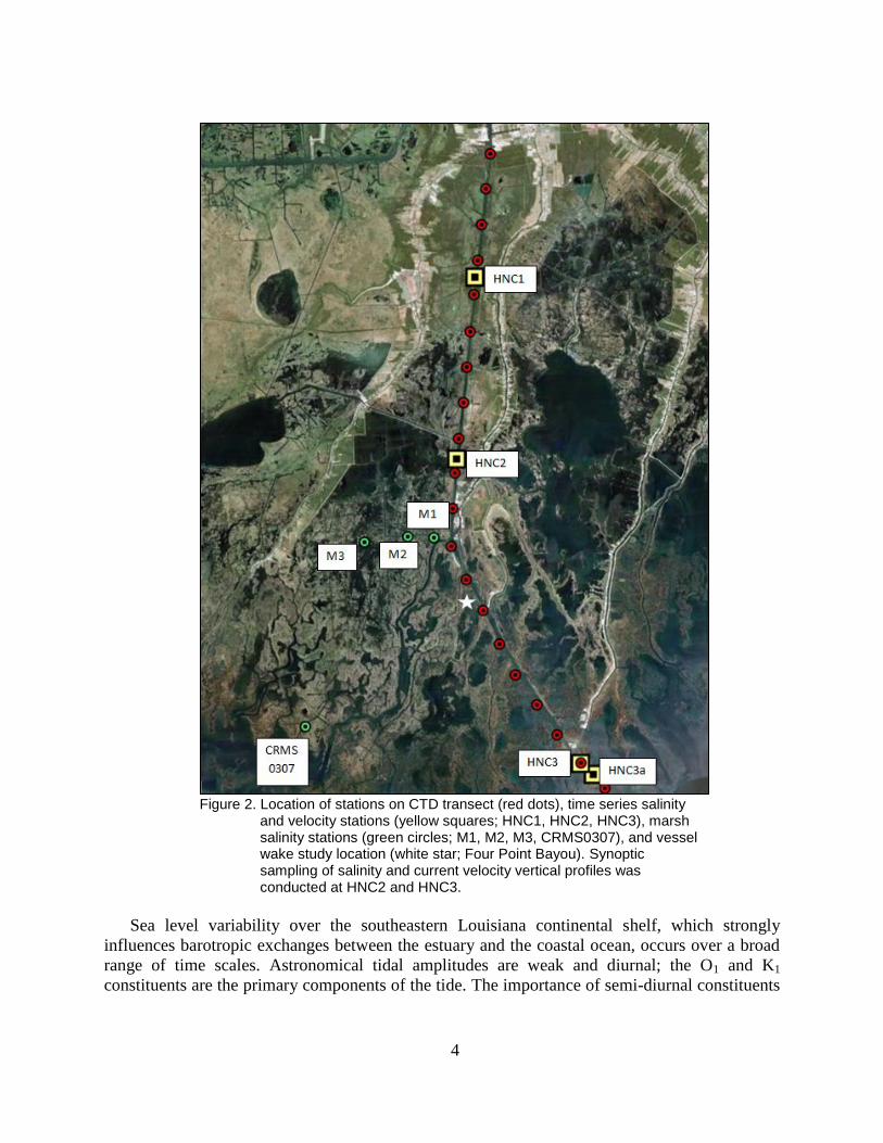
Figure 2. Location of stations on CTD transect (red dots), time series salinity
and velocity stations (yellow squares; HNC1, HNC2, HNC3), marsh salinity stations (green circles; M1, M2, M3, CRMS0307), and vessel wake study location (white star; Four Point Bayou). Synoptic sampling of salinity and current velocity vertical profiles was conducted at HNC2 and HNC3.
Sea level variability over the southeastern Louisiana continental shelf, which strongly
influences barotropic exchanges between the estuary and the coastal ocean, occurs over a broad
range of time scales. Astronomical tidal amplitudes are weak and diurnal; the O1 and K1
constituents are the primary components of the tide. The importance of semi-diurnal constituents
5
(e.g., M2, S2) in the overall astronomical tidal fluctuations along the northern and eastern coasts
of the GOM is minimal. One important implication of the dominance of the diurnal constituents
in this region is that the fortnightly cycle in tidal amplitude results from an offset of the plane of
the moon’s orbit relative to the earth’s equator. This 13.66-day tropic-equatorial cycle is
physically distinct from the 14.8-day spring-neap cycle in tidal amplitude that occurs in semi-
diurnal regimes as a result of varying positions of the sun and the moon relative to the earth.
Over timescales of a few days, wind stress becomes important in regulating estuary-shelf
exchanges, particularly during autumn and winter when the passage of winter storm systems
occurs every 4–7 days (Chuang and Wiseman 1983) and this storm-induced wind stress causes
shelf sea levels to fluctuate with typical amplitudes of approximately 0.5 m.
In “Influence of the Houma Navigation Canal on Salinity Patterns and Landscape
Configuration in Coastal Louisiana,” Steyer et al. (2008) evaluated how the HNC may have
contributed to the increased salinity and land loss that has occurred in the marshes that surround
it. This 2008 study examined the patterns of marsh deterioration as a function of hydrological
connectivity to higher salinity waters. Due to lack of current data and models, no direct
relationship was detected because of high variability of land loss in the marshes adjacent to
(within 3 km) the HNC. Although the HNC may have influenced marsh degradation in some
fashion, the degree and distance to which that influence manifested itself could not be
determined by the study.
Understanding how the circulation and mixing processes in the HNC influence the exchange
of salt between the Terrebonne marshes and the coastal ocean, and how these processes are
modulated by external physical processes, is critical to anticipating the effects of future actions
and circumstances such as deepening the channel, placing locks in the channel, changes in
freshwater discharge down the channel, and sea level rise. Though weak tidal stirring (e.g.,
equatorial tides) and strong buoyancy forcing (e.g., high freshwater inputs) can each enhance
stratification and subsequent gravitational circulation, (Griffin and LeBlond 1990; Ribeiro et al.
2004), their effects on vertically-averaged advective salt transport are typically opposite.
Stratification associated with weak tidal stirring tends to impede downestuary salt transport,
while stratification associated with buoyancy forcing tends to enhance it (Medeiros and Kjerfve
2005; Miranda et al. 2005). Periods of increased marsh salinities may result from prolonged
episodes of strong upestuary salt flux in the HNC, and, thus, it is critical to understand how this
salt flux changes with varying conditions.
This study investigates variability in the salinity field and salt flux in the HNC and
surrounding marshes, and how external physical factors such as wind forcing, buoyancy forcing,
and mixing from tidal stirring may influence dispersive and advective fluxes through the HNC.
Also investigated is the relative degree to which the surrounding marshes respond to fluctuations
of salinity in the middle reaches of the HNC compared with their response to salinity variability
in the bays of the lower Terrebonne basin that propagate landward through the marshes.

7
2. METHODS
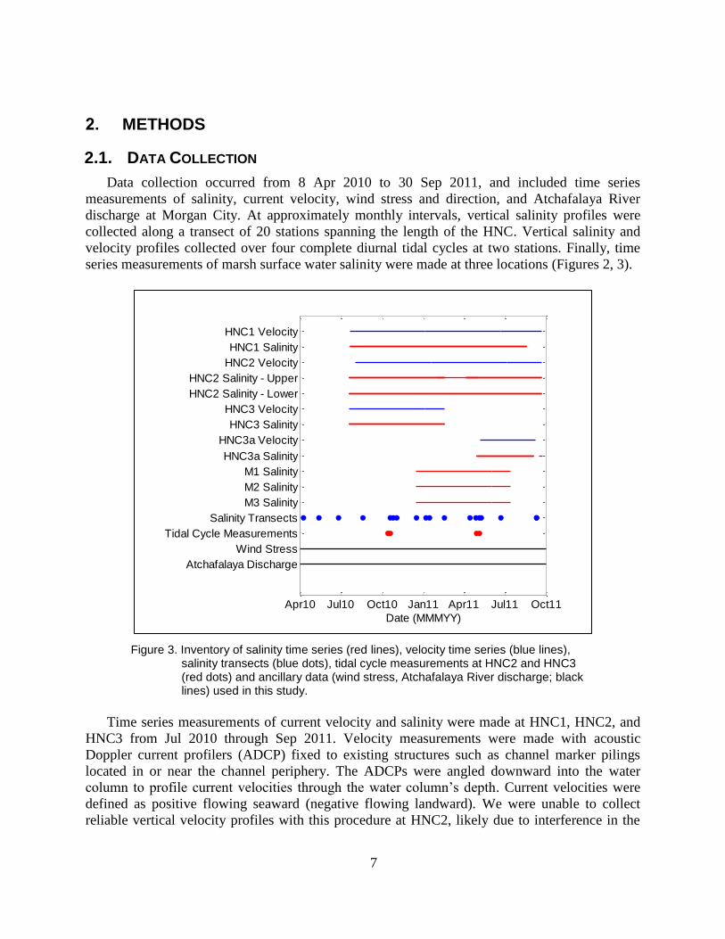
2.1. DATA COLLECTION
Data collection occurred from 8 Apr 2010 to 30 Sep 2011, and included time series
measurements of salinity, current velocity, wind stress and direction, and Atchafalaya River
discharge at Morgan City. At approximately monthly intervals, vertical salinity profiles were
collected along a transect of 20 stations spanning the length of the HNC. Vertical salinity and
velocity profiles collected over four complete diurnal tidal cycles at two stations. Finally, time
series measurements of marsh surface water salinity were made at three locations (Figures 2, 3).
Figure 3. Inventory of salinity time series (red lines), velocity time series (blue lines), salinity transects (blue dots), tidal cycle measurements at HNC2 and HNC3 (red dots) and ancillary data (wind stress, Atchafalaya River discharge; black lines) used in this study.
Time series measurements of current velocity and salinity were made at HNC1, HNC2, and
HNC3 from Jul 2010 through Sep 2011. Velocity measurements were made with acoustic
Doppler current profilers (ADCP) fixed to existing structures such as channel marker pilings
located in or near the channel periphery. The ADCPs were angled downward into the water
column to profile current velocities through the water column’s depth. Current velocities were
defined as positive flowing seaward (negative flowing landward). We were unable to collect
reliable vertical velocity profiles with this procedure at HNC2, likely due to interference in the
Apr10 Jul10 Oct10 Jan11 Apr11 Jul11 Oct11
HNC1 Velocity
HNC1 Salinity
HNC2 Velocity
HNC2 Salinity - Upper
HNC2 Salinity - Lower
HNC3 Velocity
HNC3 Salinity
HNC3a Velocity
HNC3a Salinity
M1 Salinity
M2 Salinity
M3 Salinity
Salinity Transects
Tidal Cycle Measurements
Wind Stress
Atchafalaya Discharge
Date (MMMYY)
8
flow field caused by the presence of wing walls and other structures associated with the nearby
Dulac pontoon bridge. Complete velocity datasets were obtained at HNC1 and HNC2. The
channel marker containing the instrumentation at HNC3 was presumably hit by a large vessel
sometime between Feb and Apr 2011, and all instrumentation at this station was lost, along with
data collected during that deployment. A new station, HNC3a, was established on 5 May 2011
and collected data until 6 Sep 2011, the date of the last data retrieval trip before it appeared to be
damaged during Tropical Storm Lee.
Salinity time series measurements were made near the surface at HNC1, HNC2, and HNC3,
and also near the bottom of the water column at HNC2 (Figures 2, 3). Collection of near-surface
and near-bottom salinity at HNC2 allowed for the computation of vertical salinity stratification
during the study (calculated as the difference between bottom and surface salinity). In addition to
HNC1, HNC2, and HNC3, three marsh stations (M1, M2, M3) were established to quantify
salinity variability in the marshes surrounding the HNC, as well as in a major channel that
provides a conduit for salt delivery from the HNC to these marshes (Figures 2, 3). Wind stress
and direction were also collected every 15 minutes at HNC2.
Vertical salinity profiles along a transect spanning the length of the HNC were collected
approximately monthly from April 2010 to September 2011 with a YSI CastAway conductivity-
temperature-depth (CTD) profiler (Figures 2, 3). The CTD profiler samples at 5 Hz, and sinks
through the water column at approximately 1 m/s, providing a salinity data point approximately
every 20 cm. The transect consisted of 20 stations spaced every 2 km, and for each survey all
salinity data points were interpolated horizontally and vertically to provide depth-length salinity
contours for the transect. Each transect took approximately 1.5 hours to complete, so temporal
changes in the salinity field between the onset and completion of the transect associated with the
diurnal tide were minimal.
Vertical profiles of hydrographic properties and current velocity were collected over
complete diurnal tidal cycles at HNC2 and HNC3 with a YSI CastAway CTD profiler and a
SonTek RiverSurveyor M9 ADCP (Figures 2, 3). This sampling was conducted during low (Oct
2010) and high (Apr–May 2011) Atchafalaya River flow conditions during tropic (13–14 Oct
2010; 5–6 May 2011) and equatorial (19–20 Oct 2010; 28–29 Apr 2011) phases of the
fortnightly tidal cycle.
To measure the impact that vessel wakes had on transmitting salt from the HNC into the
marshes through adjoining waterways, a short experiment was set up on 3 Jul 2012 in Four Point
Bayou, roughly 100 m from its confluence with the HNC (Figures 2, 3). At this site, salinity and
velocity were measured every minute for a 3.25-h deployment. It was assumed that salinity and
velocity were homogenous throughout the channel’s cross-section, and salt flux through the
channel was taken as the product of velocity and salinity (expressed as psu m/s). Impacts of
vessel wakes on salt transport were assessed by examining deviations from background levels of
salt fluxes (e.g., tidal, wind-induced) when wakes from vessels using in the HNC entered Four
Point Bayou and passed the instrumentation.
9
2.2. DATA ANALYSIS
Fourier analysis (Bendat and Piersol 1986) has been widely used to examine periodicities in
geophysical time series, and is useful if underlying processes are stationary through time.
However, geophysical data are often nonstationary, meaning that the nature of their signals can
change through time. The wavelet transform can be used to analyze time series data that contain
nonstationary variability that occurs over multiple timescales (Daubechies 1990). This approach
has been used in numerous studies of geophysics, including the El Nino southern Oscillation
(ENSO; Torrence and Webster 1999; Jevrejeva et al. 2003), river discharges (Labat et al. 2004),
sea level changes (Jevrejeva et al. 2005), and precipitation variability (Kayano and Andreoli
2006).
A wavelet is a function with zero mean that is localized in both time and frequency. One
particular wavelet, the Morlet, is defined as
( )
(1)
where ωo is dimensionless frequency and η is dimensionless time. This wavelet is a complex
wave ( ) within a Gaussian envelop ( ), which localizes the wavelet in time. The
wavelet transform of a time series (xn, n = 1, 2, …, N) with uniform time steps δt is defined as the
convolution of xn with the scaled and translated wavelet,
( ) √
∑ [( )
]
(2)
where s is timescale. Like the Fourier power spectrum, the wavelet power spectrum is defined as
the absolute value squared of the wavelet transform ( | | ). In simple terms, the wavelet
spectrum provides an estimate of variance for a time series as a function of time and timescale of
variability (see Appendix 1). It does so by measuring localized sinusoidal variance over varying
timescales throughout the duration of a time series.
Because the length of time series records is finite, errors occur at the left and right regions of
the wavelet spectrum. To cope with the boundaries of time series, each end of the time series is
padded with zeroes. This procedure introduces discontinuities and decreases variance at the ends
of the time series. The region of the wavelet spectrum where these issues occur are termed the
cone of influence, and caution should be made in these regions as it is uncertain whether
decreases in variance are due to true decreases in the signal or are simply artifacts of zero
padding.
Given two time series x and y, with wavelet transforms Wx (t, s) and Wy (t, s), the cross-
wavelet transform is defined as Wxy (t, s) = Wx (t, s) · Wy (t, s)*, where * indicates the complex
conjugate of the preceding quantity. The cross-wavelet power spectrum is then | ( )| .
Cross-wavelet power indicates regions in time-frequency space where two time series share high
variance. The cross-wavelet transform can be used to compute the wavelet coherence, which
indicates the localized correlation between two time series in time-frequency space, estimated as
10
( ) |⟨ ( )⟩|
⟨ | ( )| ⟩ ⟨ | ( )| ⟩ (3)
where ⟨ ⟩ indicates smoothing in both time and scale. Bearing in mind that the definition of the
wavelet coherence spectrum closely resembles that of a traditional correlation coefficient, it is
useful to consider it as a localized correlation coefficient in time-frequency space. Finally, the
wavelet phase spectrum is estimated as
( ) ( {⟨ ⟩}
{⟨ ⟩}) (4)
where Im and Re indicate taking the imaginary and real components of the following complex
quantity, respectively. The phase spectrum provides an indication of the relative timing of the
two time series in question, that is, by how much time y lags or leads x.
11
3. RESULTS AND DISCUSSION
3.1. TIDAL VARIABILITY
Estimates of tidal constituent amplitude and phase for depth-averaged current velocity at
HNC1, HNC 2, and HNC3 were obtained with least-squares harmonic analysis (Dronkers 1964;
Table 1). Currents were oriented along the HNC’s length, and tidal fluctuations accounted for
greater than 84% of the total current variability at HNC3, 68% at HNC2, and 39% at HNC1.
Tidal current amplitudes generally decrease inland from HNC3 in response to frictional
attenuation of tidal fluctuations. The tidal form number, calculated as the ratio of the main
diurnal to semidiurnal component amplitudes (K1+O1)/(M2+S2), was 15.7, 17.9, and 8.9 for
HNC1, HNC2, and HNC3, respectively, and indicates that all sites could be classified as fully
diurnal (form number exceeds 3.0; Boon 2004).
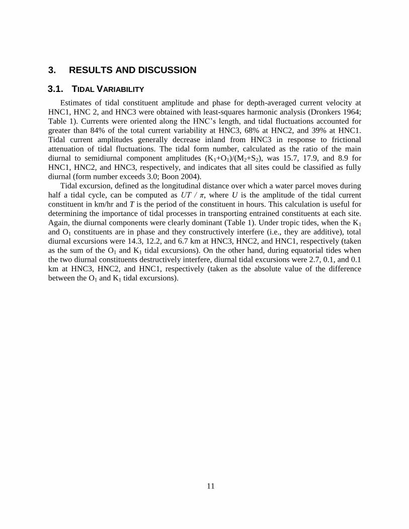
Tidal excursion, defined as the longitudinal distance over which a water parcel moves during
half a tidal cycle, can be computed as UT / π, where U is the amplitude of the tidal current
constituent in km/hr and T is the period of the constituent in hours. This calculation is useful for
determining the importance of tidal processes in transporting entrained constituents at each site.
Again, the diurnal components were clearly dominant (Table 1). Under tropic tides, when the K1
and O1 constituents are in phase and they constructively interfere (i.e., they are additive), total
diurnal excursions were 14.3, 12.2, and 6.7 km at HNC3, HNC2, and HNC1, respectively (taken
as the sum of the O1 and K1 tidal excursions). On the other hand, during equatorial tides when
the two diurnal constituents destructively interfere, diurnal tidal excursions were 2.7, 0.1, and 0.1
km at HNC3, HNC2, and HNC1, respectively (taken as the absolute value of the difference
between the O1 and K1 tidal excursions).
12
Table 1. Amplitude, phase, time lag from HNC3, and tidal excursion distances for major tidal constituents of
current velocity at HNC1, HNC2, and HNC3.
HNC1
Constituent Period
(hours)
Amplitude
(m/s)
Phase
(degrees)
Time Lag
from HNC 3
(hours)
Tidal
Excursion
(km)
O1 25.81 0.116 286 5.16 3.43
K1 23.93 0.120 131 4.52 3.29
M2 12.42 0.008 33 4.89 0.11
S2 12.00 0.007 69 4.06 0.10
HNC2
Constituent Period
(hours)
Amplitude
(m/s)
Phase
(degrees)
Time Lag
from HNC 3
(hours)
Tidal
Excursion
(km)
O1 25.81 0.208 271 4.08 6.15
K1 23.93 0.222 116 3.50 6.08
M2 12.42 0.014 356 3.65 0.20
S2 12.00 0.010 47 3.33 0.14
HNC3
Constituent Period
(hours)
Amplitude
(m/s)
Phase
(degrees)
Time Lag
from HNC 3
(hours)
Tidal
Excursion
(km)
O1 25.81 0.289 214 --- 8.51
K1 23.93 0.212 64 --- 5.81
M2 12.42 0.036 250 --- 0.50
S2 12.00 0.020 307 --- 0.25
Tidal excursions should be interpreted in the context of the geometry of the HNC. The
distance between the landward and seaward ends of the HNC is roughly 40 km. Thus, during
tropic tides, a parcel of water or entrained salt entering the HNC on the flood tide can be
expected to be transported less than halfway up the HNC before the tide reverses itself. Though
the tropic tidal excursion distances were considerably less than the length of the channel, they
were still roughly the same order of magnitude (tens of kilometers), and thus one can expect tidal
dispersion to be an important physical process with regard to the import of salt (Geyer and
Signell 1992). During equatorial tides, the excursions were roughly an order of magnitude less,
and other forms of transport, such as gravitationally- or meteorologically-induced changes, likely
become more important.
13
3.2. SUBTIDAL CURRENT VARIABILITY
Subtidal mid-depth current velocity fluctuations at HNC1, HNC2, and HNC3 were obtained
by removing tidal-frequency variability from each current velocity time series record with a
Lanczos lowpass filter with a 40-hr half-amplitude cutoff period. Mean subtidal current
velocities ranged from 13.0 cm/s at HNC1 to 5.7 cm/s at HNC3. Though subtidal currents were
oscillatory in nature, they were primarily directed seaward. This was particularly true at HNC1
and HNC2 (Figure 4). All three sites exhibited the same general pattern of a period of high
variability over 3–10 day timescales between Nov 2010 and May 2011 (Figure 5), consistent
with synoptic weather forcing of subtidal flow associated with the passage of winter storms.
Current velocity was coherent with along- and cross-shelf wind stress at HNC1 and HNC2
(Figure 6). Phase between alongshelf winds and current velocity at HNC1 and HNC2 was near
0º, indicating that winds blowing toward the east tended to facilitate seaward flow (Figure 6).
Phase between cross-shelf wind and current velocity was near 180º, indicating that a negative
(landward) current was induced by a positive (northward) cross-shelf wind stress. In other words,
winds blowing toward the east and south tend to force flow out of the HNC; winds blowing
toward the west and north tend to force flow into the HNC. Coherence with wind stress
components at HNC1 and HNC2 was greatest over 3–10 day periods, indicating that cycles of
wind-forced exchanges tended to recur every 3–10 days. Coherence analysis between wind stress
and HNC3/HNC3a could not be calculated across the entire dataset due to a nearly three-month
gap in the dataset that occurred following loss of the channel marker that housed the
instrumentation for HNC3. Dynamics related to HNC3 based on a shorter dataset are presented
below.
Figure 4. Mean subtidal water column velocity at HNC1 (top), HNC2 (middle), HNC3 (first time series, bottom), and HNC3a (second time series, bottom).
14
Figure 5. Wavelet power spectra for depth-averaged current velocity at HNC1 (left), HNC2 (middle) and HNC3/HNC3a
(right). In each plot, the time-evolution of wavelet power, normalized to the time series variance, is shown by the contour plot in the upper left. To the right of each contour plot is the global wavelet spectrum for each time series (wavelet power averaged through time). Below each contour plot is a plot of the actual time series. The global wavelet spectrum for HNC3/HNC3a was not calculated because a lengthy gap in the time series made its computation impossible.
.
15
Figure 6. Wavelet coherence and phase spectra of seaward current velocity at HNC1 (upper) and HNC2 (lower) with alongshore (left) and cross-shore (right) wind stress. Solid lines delineate regions of time-frequency space where coherence between the time series is significant at α = 0.05. Phase is indicated by the direction of the arrows, where an arrow pointing toward the right indicates an in-phase (positive with little or no time lag) relation, an arrow pointing down indicates current lags wind stress by 90˚, and arrow to the left indicates the two time series are out of phase by 90˚ (inverse relation with little or no lag) and an upward pointing arrow indicates current velocity leads wind stress.
3.3 VERTICAL VARIATION IN SUBTIDAL VELOCITY STRUCTURE AT HNC1 AND
HNC3
The top panel of Figure 7 shows near surface and near bottom subtidal current velocities at
HNC3. Subtidal currents usually did not exceed 0.4 m/s, and though the currents appeared to be
largely depth-independent, there were several brief episodes where considerable vertical current
shear was evident. The lower portion of Figure 7 shows wind stress during the study. Winds
were generally light and variable through mid-September, and then transitioned to strong,
predominantly southward by late October. The passage of several winter frontal systems is
evident between this time and the remainder of the data collection period at HNC3 (16 Feb
2011).
16
Figure 7. Time series of subtidal current velocities at HNC3 (upper panel; blue line represents near-surface currents, red line represents near-bottom currents). Vector plot of wind stress at HNC2 (lower panel). A vector extending upwards from the x-axis indicates wind blowing from the north; a vector extending leftward from the x-axis indicates wind blowing from the west. Vector length indicates magnitude of wind stress.
Empirical orthogonal function (EOF) analysis (Priesendorfer 1988) was performed on the
HNC3 current velocity data set to provide a compact description of the dominant modes of
vertical variation of currents in the lower HNC. EOF analysis optimally partitions the variance of
a field into orthogonal vertical patterns (modes) that are simply the eigenvectors of the data
field’s covariance matrix. Each mode is associated with a corresponding eigenvalue that is
proportional to its percentage of the total variance in the dataset. Each mode is also associated
with a time series (principal component; PC) that describes the EOF’s evolution through time.
EOF solutions were normalized to their standard deviations, giving each principal component a
variance of unity and, thus, amplitudes on each eigenvector carry units in m/s, and amplitudes
associated with each PC are dimensionless quantities.
The first two modes accounted for 99.6% of the total subtidal flow variability at HNC3.
Thus, nearly all of the variability expressed by ten time series (one time series for each velocity
bin) could be conveyed by two PC time series and their associated EOF modes. Over 90% of the
total variability could be attributed to mode-1, which carries the same sign throughout the water
column, with a slight magnitude decrease with increasing depth (Figure 8, upper left). Hence,
mode-1 depicts currents at HNC3 in which the direction of the flow does not vary with depth,
and serves as a metric of barotropic exchanges (driven by sea-surface elevation gradients) that
occur in the lower HNC between Terrebonne Bay and the wetlands to its north. Mode-2
accounted for slightly greater than 8% of the total flow field variability. Unlike the mode-1, a
reversal in sign at roughly mid-depth exists in the eigenvector for mode-2 (Figure 8, lower left),
and mode-2 hence represents flow at HNC3 where the surface currents opposed those at the
bottom. Thus, mode-2 describes a vertically-sheared flow through the lower HNC, similar to
baroclinic currents associated with gravitational circulation driven by a horizontal density
gradient. None of the remaining 8 modes comprise greater than 0.2% of the total flow variability.
17
Figure 8. Vertical distributions of EOF eigenvector amplitudes (left) and principal component time series (right) for EOF modes 1 (upper; barotropic) and 2 (lower; baroclinic) at HNC3. The EOF solutions have been normalized so that the eigenvector amplitudes have units of m/s and the principal component time series have a non-dimensional variance of unity. Positive values indicate seaward flow, negative values indicate landward flow.
Positive values for the time series describing the temporal evolution of the mode-1 response
(PC1) indicate outflows and negative values indicate inflows past HNC3 (Figure 8, upper right).
From Jul 2010 to early Oct 2010, a significant variance peak with a period near 20-day exists
(Figure 9). Beginning in November and extending through the remainder of the data collection
period, the dominant timescale of wind forcing shifted from 20 days to 3–10 days, and the
variance associated with these 3–10 day oscillations in the amplitude of PC1 increased.
-0.1 0 0.1
0
.5
1
0
.5
1
No
rma
lize
d D
ep
th
Velocity (m/s)
-0.1 0 0.1
0
.5
1
0
.5
1
Velocity (m/s)
No
rma
lize
d D
ep
th
Aug10 Sep10 Oct10 Nov10 Dec10 Jan11 Feb11
-0.5
0
0.5
Date(MMMYY)
Am
plitu
de
Aug10 Sep10 Oct10 Nov10 Dec10 Jan11 Feb11
-0.5
0
0.5
Date (MMMYY)
Am
plitu
de
18
Figure 9. Wavelet power spectrum (upper left), global wavelet spectrum (right) and time series (bottom) for PC1. Positive values for PC1 time series indicate barotropic outflows, negative values indicate barotropic inflows.
Because wind forcing is largely responsible for subtidal barotropic exchanges between
estuaries and continental margins, coherence spectra (Bendat and Piersol 1986) were estimated
between PC1 and each directional component of wind stress between 0 and 180ºT (0˚T being
true north) at 5º increments (Figure 10). For each frequency, the direction of maximum
coherence θ was determined as
| || |
| | | | (5)
(Garrett and Toulany 1982), where h1 and h2 are partial transfer functions relating orthogonal
wind stress components, in this case eastward and northward, to PC1 and φ is the phase
difference between h1 and h2. Variability in PC1 was most coherent along the 90–270ºT
component (τ90), and the wavelet spectrum of τ90 is very similar to that of PC1, with a region of
high variance over roughly 20-day periods between July and October, after which the dominant
period of variability shifted to 3–10 day periods (Figure 11). Cross-wavelet analysis was used to
investigate the influence that τ90 exerted on barotropic flows at HNC1 (Figure 12). High
coherence (>0.8) existed across regions of time-frequency space where variability for both PC1
and τ90 were high, and phase in these regions was near zero, indicating that winds blowing
toward the east (90ºT) were associated with positive values of PC1 (barotropic outflows) at
HNC3.
19
Figure 10. Coherence squared between PC1 and wind stress components along the directions of -90˚T–90˚T in 5˚ increments, obtained from cross-spectral analysis (Bendat and Piersol 1986). The dashed line indicates the direction of maximum wind forcing, estimated according to Garrett and Toulany (1982).
Figure 11. Wavelet power spectrum (upper left), global wavelet spectrum (right) and time series (bottom) for τ90. Positive values for τ90time series indicate wind blowing toward east, negative values indicate wind blowing toward west.
20
Figure 12. Wavelet coherence and phase between τ90 and PC1.
The time series describing the temporal pattern of the sheared flow response (PC2) nearly
always carries a positive sign (Figure 8, lower right), Thus, flows associated with mode-2 can be
characterized by outflow in the upper water column, and inflows near the bottom, and resemble
what one might expect from traditional baroclinic estuarine circulation theory. The wavelet
power spectrum for PC2 (Figure 13) shows strong variability exists across timescales of 10–20
days from July through October. The variability over this time scale then diminishes through
early January, and then returns for the remainder of the record.
21
Figure 13. Wavelet power spectrum (upper left), global wavelet spectrum (right) and time series (bottom) for PC2. Positive values for PC2 time series indicate surface outflow and bottom inflow, negative values indicate surface inflow and bottom outflow.
Because horizontal salinity gradients and variability in tidal current amplitude have been
shown to strongly influence the strength of gravitational circulation, a two-input partial cross-
wavelet model was used to investigate the combined role of the horizontal salinity gradient and
diurnal tidal current amplitude in regulating gravitational circulation (PC2) at HNC3. The
horizontal salinity gradient was taken as the difference in salinity between Terrebonne Bay and
HNC2, while the diurnal tidal current amplitude was estimated with complex demodulation
(Bloomfield 1976). Complex demodulation estimates the time evolution of the amplitude of a
time series at a specified frequency fo. Here the diurnal tidal frequency is to be enveloped, so fo is
taken as 0.0403 cycles/hr, which is at the center of a frequency band that spans the frequencies of
the O1 and K1 tidal constituents. Multiplication of the current velocity time series by a complex
exponential of frequency fo gives ( ) ( ) (6)
This procedure frequency-shifts the data, which can then be smoothed with a low-pass filter to
eliminate higher-frequency fluctuations not associated with fo. Here, a low-pass Lanczos filter
with a half-amplitude cutoff period of 120 hours was used. Variability in the resulting complex
time series Ud (t, fo) in a band near the central frequency (in this case the diurnal tide) can now be
expressed in terms of a time-varying amplitude | ( )|, where brackets indicate absolute
value.
The time series of the horizontal density gradient between Terrebonne Bay and HNC2, along
with its wavelet spectrum, are shown in Figure 14. The salinity gradient is always positive,
indicating higher salinities in Terrebonne Bay than at HNC2. The magnitude of the gradient
shows considerable variability, and it appears to pulse every 10–20 days early in the record and
near the latter portion of the record. The wavelet power spectrum confirms this pattern of
variability, and appears similar to the wavelet spectrum of PC2, with relatively high variability
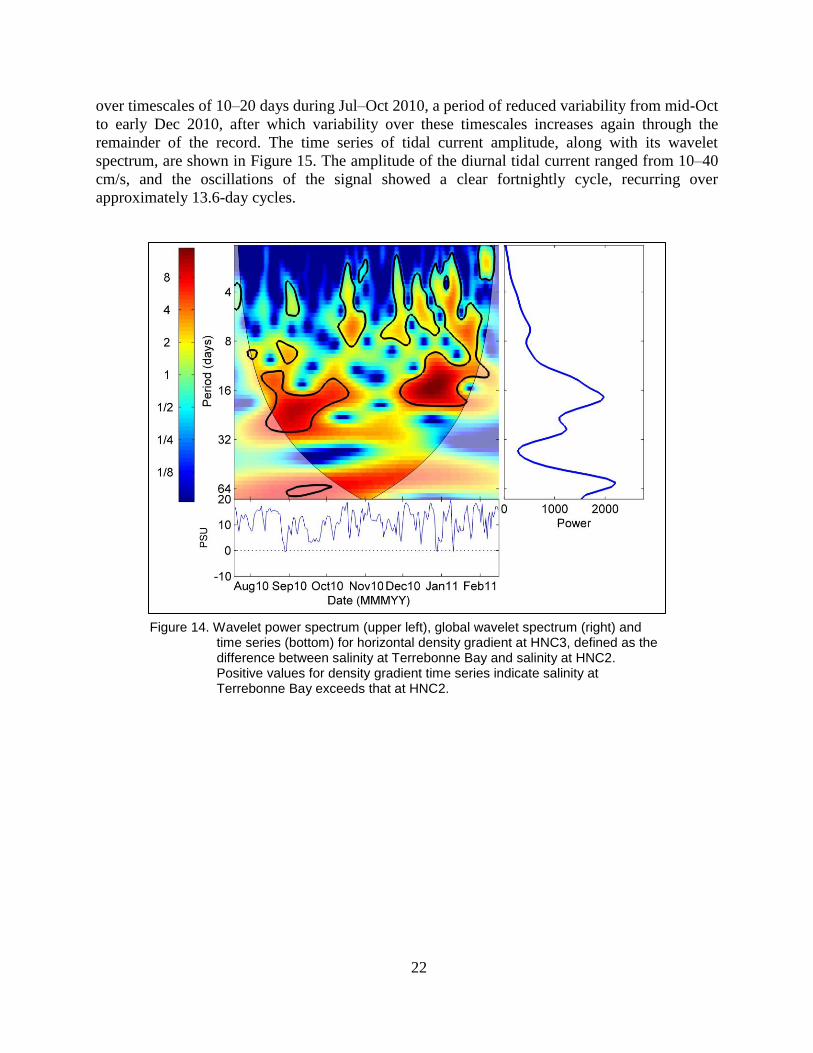
22
over timescales of 10–20 days during Jul–Oct 2010, a period of reduced variability from mid-Oct
to early Dec 2010, after which variability over these timescales increases again through the
remainder of the record. The time series of tidal current amplitude, along with its wavelet
spectrum, are shown in Figure 15. The amplitude of the diurnal tidal current ranged from 10–40
cm/s, and the oscillations of the signal showed a clear fortnightly cycle, recurring over
approximately 13.6-day cycles.
Figure 14. Wavelet power spectrum (upper left), global wavelet spectrum (right) and
time series (bottom) for horizontal density gradient at HNC3, defined as the difference between salinity at Terrebonne Bay and salinity at HNC2. Positive values for density gradient time series indicate salinity at Terrebonne Bay exceeds that at HNC2.
23
Figure 15. Wavelet power spectrum (upper left), global wavelet spectrum (right) and time series (bottom) for diurnal tidal current amplitude at HNC3. The white horizontal line through the wavelet power spectrum indicates 13.6 days, the beat period of the O1 and K1 tidal constituents and the period over which the diurnal tide transitions from equatorial to tropic and back to equatorial.
The partial wavelet coherence spectrum between the horizontal salinity gradient and PC2
(Figure 16) indicates that these two variables were strongly coherent over timescales of 5–20
days between July and early November. Phase in these coherent regions of time-frequency space
was generally near zero, or slightly negative, indicating that PC2 variability slightly lagged that
of the horizontal density gradient, indicating that increases in the horizontal density gradient are
associated with increases in the prevalence of gravitational circulation. Coherence also exists
between the tidal current amplitude at HNC3 and PC2 (Figure 17), and is centered very closely
over 13.6 days, the beat frequency of the O1 and K1 tidal constituents and the period over which
the tropic-equatorial tidal cycle recurs. The phase between tidal current amplitude and PC2 is
near 180º, indicating that gravitation circulation is inhibited when tidal currents are strong.
Together, these results illustrate that gravitational circulation is strongest when the horizontal
salinity gradient is large during equatorial tides (weak tidal currents).
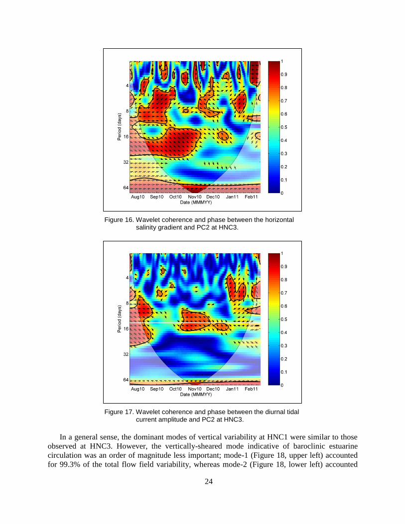
24
Figure 16. Wavelet coherence and phase between the horizontal salinity gradient and PC2 at HNC3.
Figure 17. Wavelet coherence and phase between the diurnal tidal current amplitude and PC2 at HNC3.
In a general sense, the dominant modes of vertical variability at HNC1 were similar to those
observed at HNC3. However, the vertically-sheared mode indicative of baroclinic estuarine
circulation was an order of magnitude less important; mode-1 (Figure 18, upper left) accounted
for 99.3% of the total flow field variability, whereas mode-2 (Figure 18, lower left) accounted
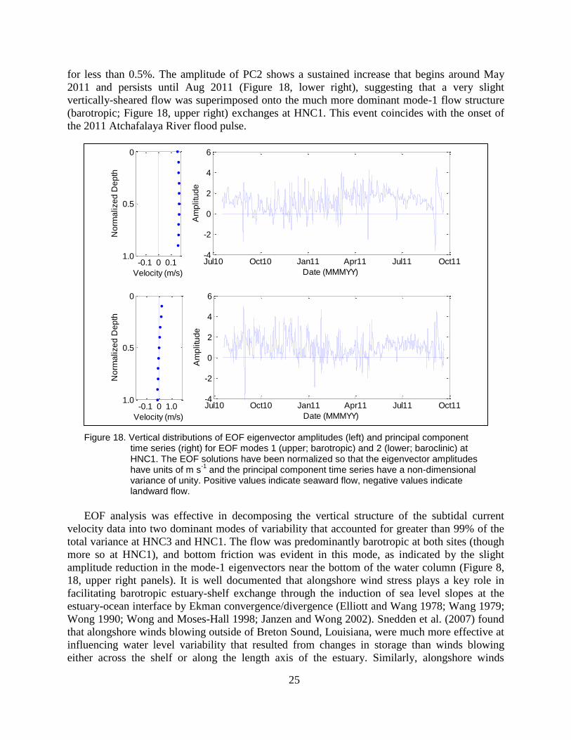
25
for less than 0.5%. The amplitude of PC2 shows a sustained increase that begins around May
2011 and persists until Aug 2011 (Figure 18, lower right), suggesting that a very slight
vertically-sheared flow was superimposed onto the much more dominant mode-1 flow structure
(barotropic; Figure 18, upper right) exchanges at HNC1. This event coincides with the onset of
the 2011 Atchafalaya River flood pulse.
Figure 18. Vertical distributions of EOF eigenvector amplitudes (left) and principal component time series (right) for EOF modes 1 (upper; barotropic) and 2 (lower; baroclinic) at HNC1. The EOF solutions have been normalized so that the eigenvector amplitudes have units of m s
-1 and the principal component time series have a non-dimensional
variance of unity. Positive values indicate seaward flow, negative values indicate landward flow.
EOF analysis was effective in decomposing the vertical structure of the subtidal current
velocity data into two dominant modes of variability that accounted for greater than 99% of the
total variance at HNC3 and HNC1. The flow was predominantly barotropic at both sites (though
more so at HNC1), and bottom friction was evident in this mode, as indicated by the slight
amplitude reduction in the mode-1 eigenvectors near the bottom of the water column (Figure 8,
18, upper right panels). It is well documented that alongshore wind stress plays a key role in
facilitating barotropic estuary-shelf exchange through the induction of sea level slopes at the
estuary-ocean interface by Ekman convergence/divergence (Elliott and Wang 1978; Wang 1979;
Wong 1990; Wong and Moses-Hall 1998; Janzen and Wong 2002). Snedden et al. (2007) found
that alongshore winds blowing outside of Breton Sound, Louisiana, were much more effective at
influencing water level variability that resulted from changes in storage than winds blowing
either across the shelf or along the length axis of the estuary. Similarly, alongshore winds
-0.1 0 0.11.0
0.5
0
Velocity (m/s)
No
rma
lize
d D
ep
th
-0.1 0 1.0
0
0.5
1.0
Velocity (m/s)
No
rma
lize
d D
ep
th
Jul10 Oct10 Jan11 Apr11 Jul11 Oct11-4
-2
0
2
4
6
Date (MMMYY)
Am
plitu
de
Jul10 Oct10 Jan11 Apr11 Jul11 Oct11-4
-2
0
2
4
6
Date (MMMYY)
Am
plitu
de
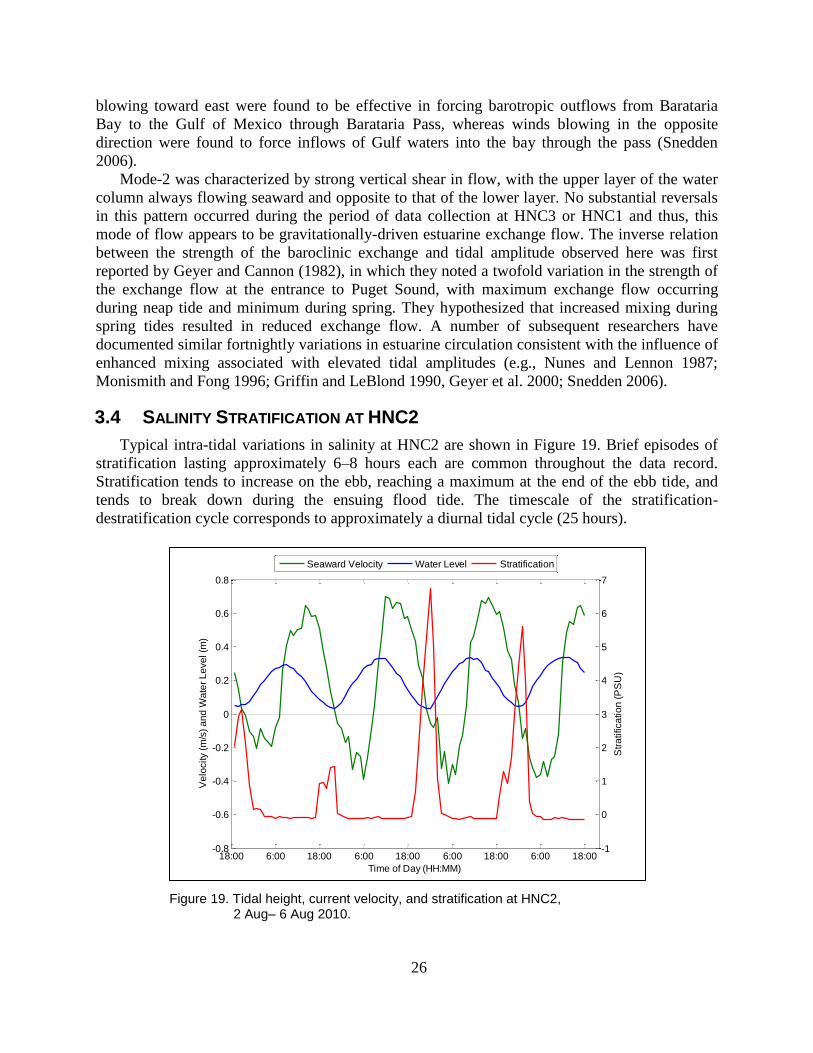
26
blowing toward east were found to be effective in forcing barotropic outflows from Barataria
Bay to the Gulf of Mexico through Barataria Pass, whereas winds blowing in the opposite
direction were found to force inflows of Gulf waters into the bay through the pass (Snedden
2006).
Mode-2 was characterized by strong vertical shear in flow, with the upper layer of the water
column always flowing seaward and opposite to that of the lower layer. No substantial reversals
in this pattern occurred during the period of data collection at HNC3 or HNC1 and thus, this
mode of flow appears to be gravitationally-driven estuarine exchange flow. The inverse relation
between the strength of the baroclinic exchange and tidal amplitude observed here was first
reported by Geyer and Cannon (1982), in which they noted a twofold variation in the strength of
the exchange flow at the entrance to Puget Sound, with maximum exchange flow occurring
during neap tide and minimum during spring. They hypothesized that increased mixing during
spring tides resulted in reduced exchange flow. A number of subsequent researchers have
documented similar fortnightly variations in estuarine circulation consistent with the influence of
enhanced mixing associated with elevated tidal amplitudes (e.g., Nunes and Lennon 1987;
Monismith and Fong 1996; Griffin and LeBlond 1990, Geyer et al. 2000; Snedden 2006).
3.4 SALINITY STRATIFICATION AT HNC2
Typical intra-tidal variations in salinity at HNC2 are shown in Figure 19. Brief episodes of
stratification lasting approximately 6–8 hours each are common throughout the data record.
Stratification tends to increase on the ebb, reaching a maximum at the end of the ebb tide, and
tends to break down during the ensuing flood tide. The timescale of the stratification-
destratification cycle corresponds to approximately a diurnal tidal cycle (25 hours).
Figure 19. Tidal height, current velocity, and stratification at HNC2, 2 Aug– 6 Aug 2010.
18:00 6:00 18:00 6:00 18:00 6:00 18:00 6:00 18:00-0.8
-0.6
-0.4
-0.2
0
0.2
0.4
0.6
0.8
Time of Day (HH:MM)
Ve
locity (
m/s
) a
nd
Wa
ter
Le
ve
l (m
)
-1
0
1
2
3
4
5
6
7
Str
atifica
tio
n (
PS
U)
Seaward Velocity Water Level Stratification
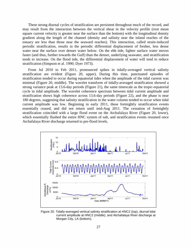
27
These strong diurnal cycles of stratification are persistent throughout much of the record, and
may result from the interaction between the vertical shear in the velocity profile (root mean
square current velocity is greater near the surface than the bottom) with the longitudinal density
gradient along the length of the channel (density and salinity near the inland reaches of the
estuary are less than those near the seaward reaches). This interaction, called strain-induced
periodic stratification, results in the periodic differential displacement of fresher, less dense
water near the surface over denser water below. On the ebb tide, lighter surface water moves
faster (and thus, further towards the Gulf) than the denser, underlying seawater, and stratification
tends to increase. On the flood tide, the differential displacement of water will tend to reduce
stratification (Simpson et al. 1990; Dyer 1973).
From Jul 2010 to Feb 2011, pronounced spikes in tidally-averaged vertical salinity
stratification are evident (Figure 20, upper). During this time, punctuated episodes of
stratification tended to occur during equatorial tides when the amplitude of the tidal current was
minimal (Figure 20, middle). The wavelet transform of tidally-averaged stratification showed a
strong variance peak at 13.6-day periods (Figure 21), the same timescale as the tropic-equatorial
cycle in tidal amplitude. The wavelet coherence spectrum between tidal current amplitude and
stratification shows high coherence across 13.6-day periods (Figure 22), and the phase is near
180 degrees, suggesting that salinity stratification in the water column tended to occur when tidal
current amplitude was low. Beginning in early 2011, these fortnightly stratification events
essentially ceased, and did not return until mid-Aug 2011. The cessation of fortnightly
stratification coincided with a large flood event on the Atchafalaya River (Figure 20, lower),
which essentially flushed the entire HNC system of salt, and stratification events resumed once
Atchafalaya River discharge returned to pre-flood levels.
Figure 20. Tidally-averaged vertical salinity stratification at HNC2 (top), diurnal tidal current amplitude at HNC2 (middle), and Atchafalaya River discharge at Morgan City, LA (bottom).
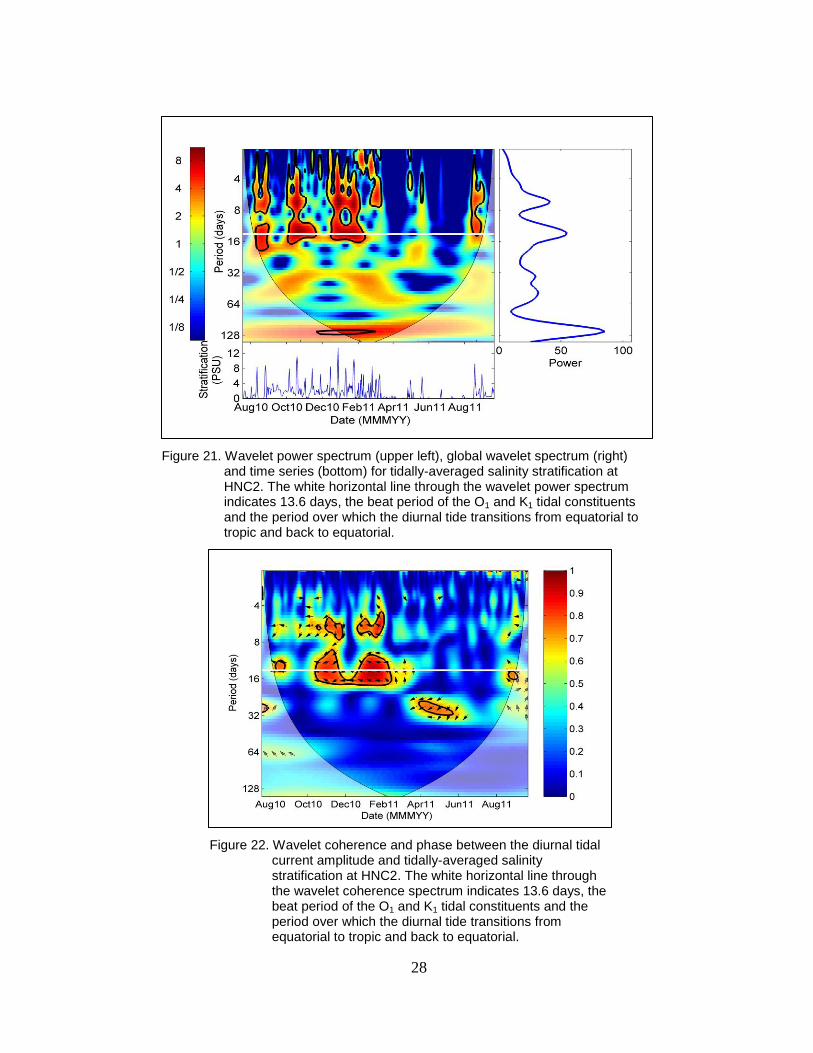
28
Figure 21. Wavelet power spectrum (upper left), global wavelet spectrum (right) and time series (bottom) for tidally-averaged salinity stratification at HNC2. The white horizontal line through the wavelet power spectrum indicates 13.6 days, the beat period of the O1 and K1 tidal constituents and the period over which the diurnal tide transitions from equatorial to tropic and back to equatorial.
Figure 22. Wavelet coherence and phase between the diurnal tidal current amplitude and tidally-averaged salinity stratification at HNC2. The white horizontal line through the wavelet coherence spectrum indicates 13.6 days, the beat period of the O1 and K1 tidal constituents and the period over which the diurnal tide transitions from equatorial to tropic and back to equatorial.
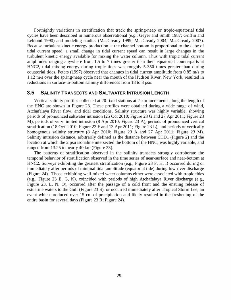
29
Fortnightly variations in stratification that track the spring-neap or tropic-equatorial tidal
cycles have been described in numerous observational (e.g., Geyer and Smith 1987; Griffin and
Leblond 1990) and modeling studies (MacCready 1999; MacCready 2004; MacCready 2007).
Because turbulent kinetic energy production at the channel bottom is proportional to the cube of
tidal current speed, a small change in tidal current speed can result in large changes in the
turbulent kinetic energy available for mixing the water column. Thus with tropic tidal current
amplitudes ranging anywhere from 1.5 to 7 times greater than their equatorial counterparts at
HNC2, tidal mixing energy during tropic tides was roughly 5-350 times greater than during
equatorial tides. Peters (1997) observed that changes in tidal current amplitude from 0.85 m/s to
1.12 m/s over the spring-neap cycle near the mouth of the Hudson River, New York, resulted in
reductions in surface-to-bottom salinity differences from 18 to 3 psu.
3.5 SALINITY TRANSECTS AND SALTWATER INTRUSION LENGTH
Vertical salinity profiles collected at 20 fixed stations at 2-km increments along the length of
the HNC are shown in Figure 23. These profiles were obtained during a wide range of wind,
Atchafalaya River flow, and tidal conditions. Salinity structure was highly variable, showing
periods of pronounced saltwater intrusion (25 Oct 2010; Figure 23 G and 27 Apr 2011; Figure 23
M), periods of very limited intrusion (8 Apr 2010; Figure 23 A), periods of pronounced vertical
stratification (18 Oct 2010; Figure 23 F and 13 Apr 2011; Figure 23 L), and periods of vertically
homogenous salinity structure (8 Apr 2010; Figure 23 A and 27 Apr 2011; Figure 23 M).
Salinity intrusion distance, arbitrarily defined as the distance between CTD1 (Figure 2) and the
location at which the 2 psu isohaline intersected the bottom of the HNC, was highly variable, and
ranged from 13.25 to nearly 40 km (Figure 23).
The patterns of stratification observed in the salinity transects strongly corroborate the
temporal behavior of stratification observed in the time series of near-surface and near-bottom at
HNC2. Surveys exhibiting the greatest stratification (e.g., Figure 23 F, H, I) occurred during or
immediately after periods of minimal tidal amplitude (equatorial tide) during low river discharge
(Figure 24). Those exhibiting well-mixed water columns either were associated with tropic tides
(e.g., Figure 23 E, G, K), coincided with periods of high Atchafalaya River discharge (e.g.,
Figure 23, L, N, O), occurred after the passage of a cold front and the ensuing release of
estuarine waters to the Gulf (Figure 23 S), or occurred immediately after Tropical Storm Lee, an
event which produced over 15 cm of precipitation and likely resulted in the freshening of the
entire basin for several days (Figure 23 R; Figure 24).
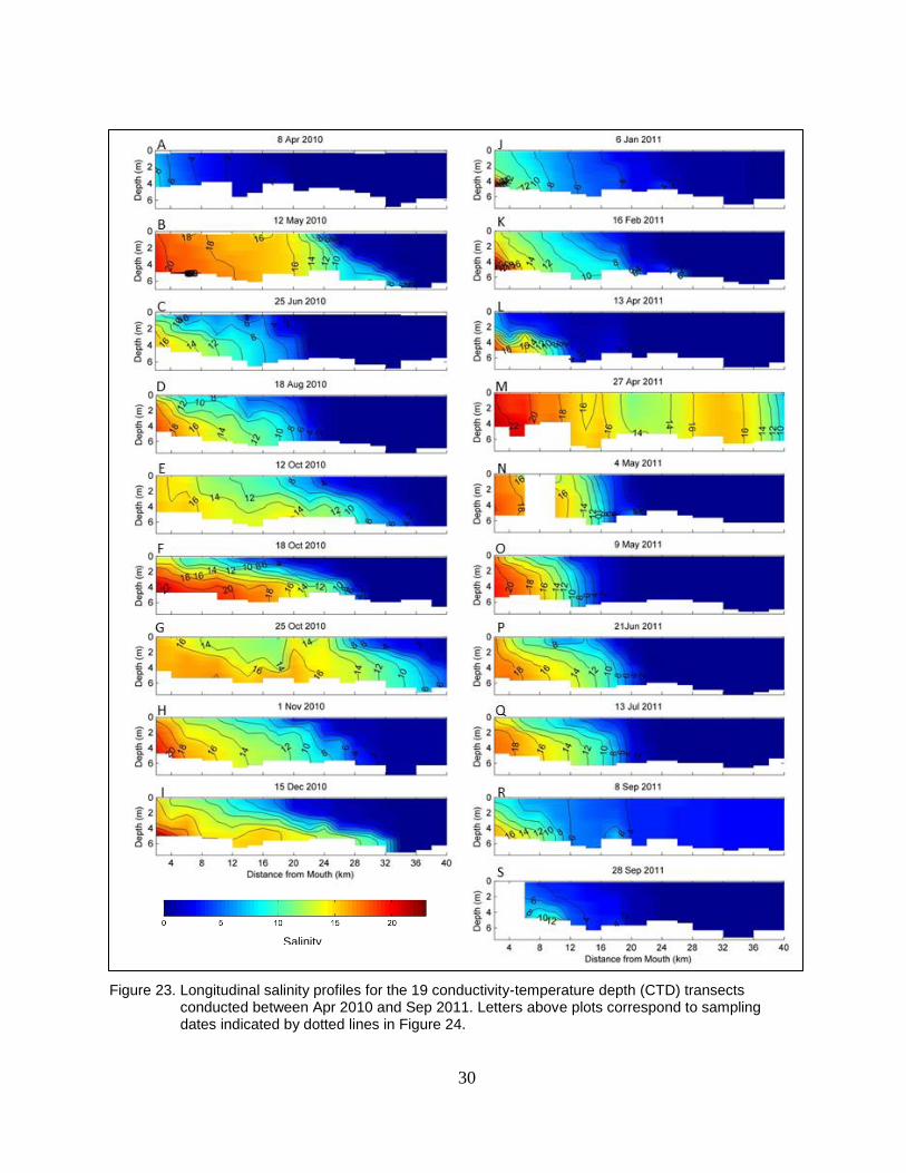
30
Figure 23. Longitudinal salinity profiles for the 19 conductivity-temperature depth (CTD) transects conducted between Apr 2010 and Sep 2011. Letters above plots correspond to sampling dates indicated by dotted lines in Figure 24.
Salinity
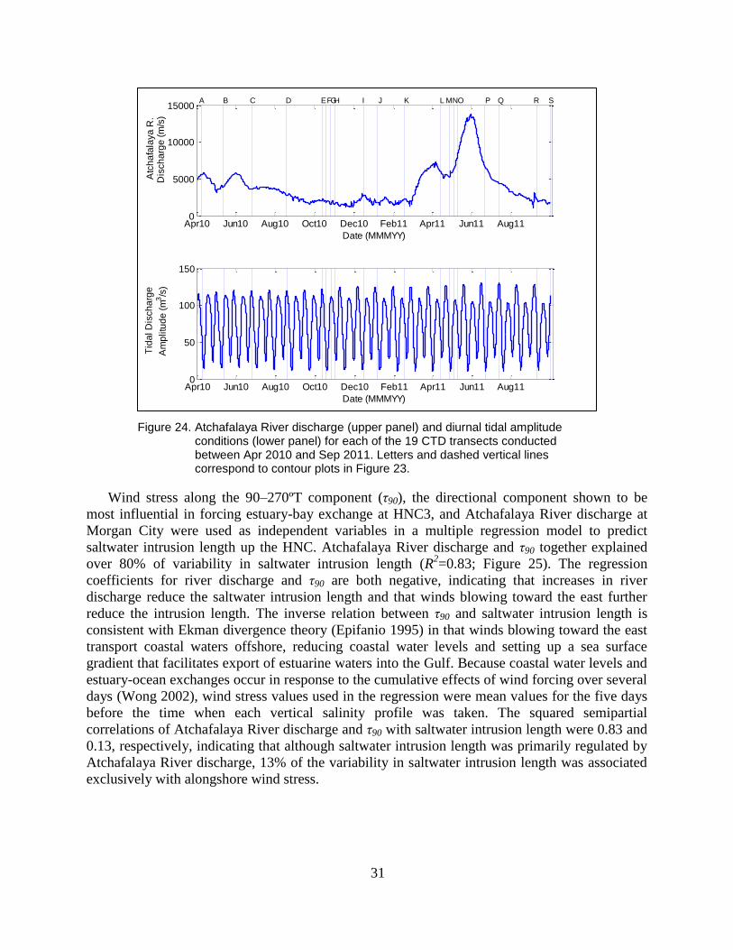
31
Figure 24. Atchafalaya River discharge (upper panel) and diurnal tidal amplitude conditions (lower panel) for each of the 19 CTD transects conducted between Apr 2010 and Sep 2011. Letters and dashed vertical lines correspond to contour plots in Figure 23.
Wind stress along the 90–270ºT component (τ90), the directional component shown to be
most influential in forcing estuary-bay exchange at HNC3, and Atchafalaya River discharge at
Morgan City were used as independent variables in a multiple regression model to predict
saltwater intrusion length up the HNC. Atchafalaya River discharge and τ90 together explained
over 80% of variability in saltwater intrusion length (R2=0.83; Figure 25). The regression
coefficients for river discharge and τ90 are both negative, indicating that increases in river
discharge reduce the saltwater intrusion length and that winds blowing toward the east further
reduce the intrusion length. The inverse relation between τ90 and saltwater intrusion length is
consistent with Ekman divergence theory (Epifanio 1995) in that winds blowing toward the east
transport coastal waters offshore, reducing coastal water levels and setting up a sea surface
gradient that facilitates export of estuarine waters into the Gulf. Because coastal water levels and
estuary-ocean exchanges occur in response to the cumulative effects of wind forcing over several
days (Wong 2002), wind stress values used in the regression were mean values for the five days
before the time when each vertical salinity profile was taken. The squared semipartial
correlations of Atchafalaya River discharge and τ90 with saltwater intrusion length were 0.83 and
0.13, respectively, indicating that although saltwater intrusion length was primarily regulated by
Atchafalaya River discharge, 13% of the variability in saltwater intrusion length was associated
exclusively with alongshore wind stress.
Apr10 Jun10 Aug10 Oct10 Dec10 Feb11 Apr11 Jun11 Aug110
5000
10000
15000
Date (MMMYY)
Atc
ha
fala
ya
R.
Dis
ch
arg
e (
m/s
)
A B C D FGH I J K L MNO P Q R SE
Apr10 Jun10 Aug10 Oct10 Dec10 Feb11 Apr11 Jun11 Aug110
50
100
150
Date (MMMYY)
Tid
al D
isch
arg
e
Am
plitu
de
(m
3/s
)
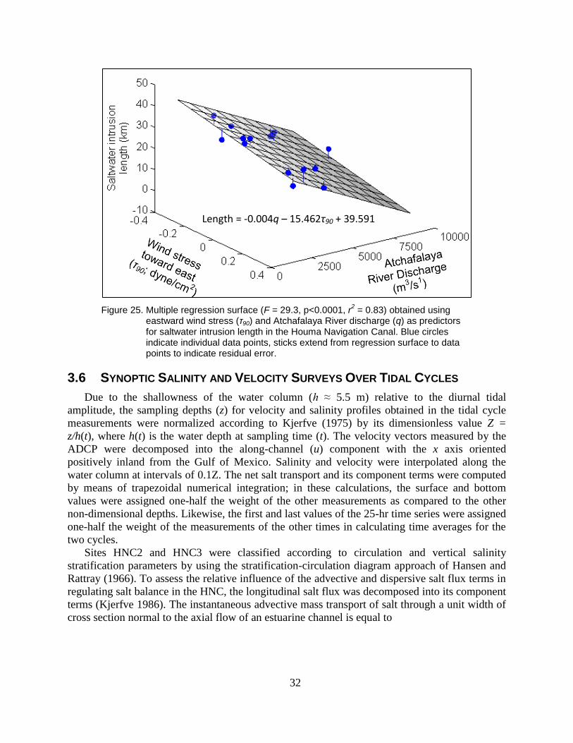
32
Figure 25. Multiple regression surface (F = 29.3, p<0.0001, r2 = 0.83) obtained using
eastward wind stress (τ90) and Atchafalaya River discharge (q) as predictors for saltwater intrusion length in the Houma Navigation Canal. Blue circles indicate individual data points, sticks extend from regression surface to data points to indicate residual error.
3.6 SYNOPTIC SALINITY AND VELOCITY SURVEYS OVER TIDAL CYCLES
Due to the shallowness of the water column (h ≈ 5.5 m) relative to the diurnal tidal
amplitude, the sampling depths (z) for velocity and salinity profiles obtained in the tidal cycle
measurements were normalized according to Kjerfve (1975) by its dimensionless value Z =
z/h(t), where h(t) is the water depth at sampling time (t). The velocity vectors measured by the
ADCP were decomposed into the along-channel (u) component with the x axis oriented
positively inland from the Gulf of Mexico. Salinity and velocity were interpolated along the
water column at intervals of 0.1Z. The net salt transport and its component terms were computed
by means of trapezoidal numerical integration; in these calculations, the surface and bottom
values were assigned one-half the weight of the other measurements as compared to the other
non-dimensional depths. Likewise, the first and last values of the 25-hr time series were assigned
one-half the weight of the measurements of the other times in calculating time averages for the
two cycles.
Sites HNC2 and HNC3 were classified according to circulation and vertical salinity
stratification parameters by using the stratification-circulation diagram approach of Hansen and
Rattray (1966). To assess the relative influence of the advective and dispersive salt flux terms in
regulating salt balance in the HNC, the longitudinal salt flux was decomposed into its component
terms (Kjerfve 1986). The instantaneous advective mass transport of salt through a unit width of
cross section normal to the axial flow of an estuarine channel is equal to
Length = -0.004q – 15.462τ90 + 39.591
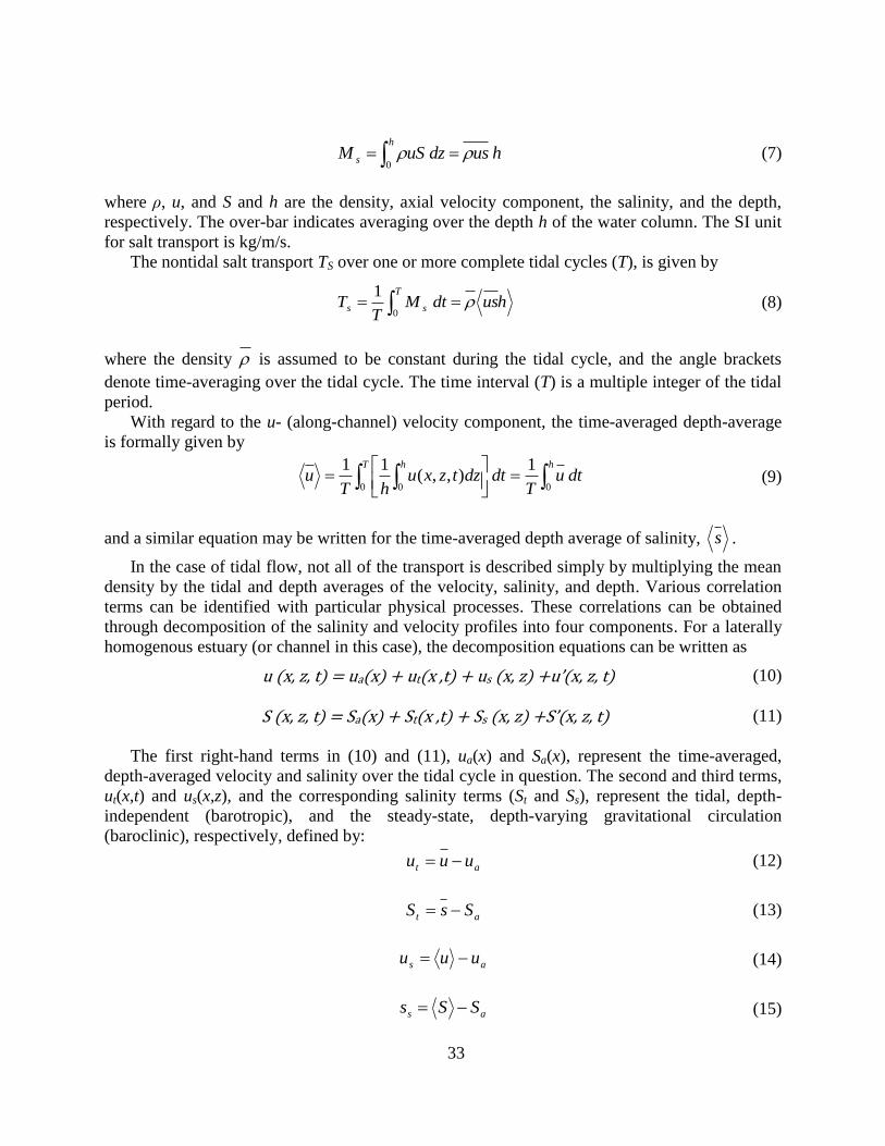
33
h
s husdzuSM0
(7)
where ρ, u, and S and h are the density, axial velocity component, the salinity, and the depth,
respectively. The over-bar indicates averaging over the depth h of the water column. The SI unit
for salt transport is kg/m/s.
The nontidal salt transport TS over one or more complete tidal cycles (T), is given by
husdtM
TT
T
ss 1
0 (8)
where the density is assumed to be constant during the tidal cycle, and the angle brackets
denote time-averaging over the tidal cycle. The time interval (T) is a multiple integer of the tidal
period.
With regard to the u- (along-channel) velocity component, the time-averaged depth-average
is formally given by
hT h
dtuT
dtdztzxuhT
u00 0
1
),,(11
(9)
and a similar equation may be written for the time-averaged depth average of salinity, s .
In the case of tidal flow, not all of the transport is described simply by multiplying the mean
density by the tidal and depth averages of the velocity, salinity, and depth. Various correlation
terms can be identified with particular physical processes. These correlations can be obtained
through decomposition of the salinity and velocity profiles into four components. For a laterally
homogenous estuary (or channel in this case), the decomposition equations can be written as
u (x, z, t) = ua(x) + ut(x ,t) + us (x z) u’(x z ) (10)
S (x, z, t) = Sa(x) + St(x ,t) + Ss (x z) S’(x z ) (11)
The first right-hand terms in (10) and (11), ua(x) and Sa(x), represent the time-averaged,
depth-averaged velocity and salinity over the tidal cycle in question. The second and third terms,
ut(x,t) and us(x,z), and the corresponding salinity terms (St and Ss), represent the tidal, depth-
independent (barotropic), and the steady-state, depth-varying gravitational circulation
(baroclinic), respectively, defined by:
at uuu
(12)
at SsS (13)
as uuu
(14)
as SSs (15)
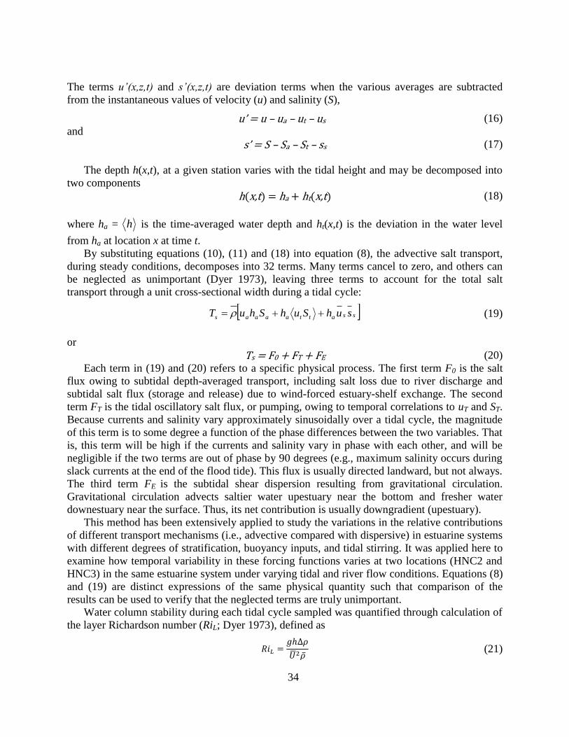
34
The terms u’(x,z,t) and s’(x,z,t) are deviation terms when the various averages are subtracted
from the instantaneous values of velocity (u) and salinity (S),
u’ u – ua – ut – us (16)
and ’ S – Sa – St – ss (17)
The depth h(x,t), at a given station varies with the tidal height and may be decomposed into
two components h(x,t) = ha + ht(x,t) (18)
where ha = h is the time-averaged water depth and ht(x,t) is the deviation in the water level
from ha at location x at time t.
By substituting equations (10), (11) and (18) into equation (8), the advective salt transport,
during steady conditions, decomposes into 32 terms. Many terms cancel to zero, and others can
be neglected as unimportant (Dyer 1973), leaving three terms to account for the total salt
transport through a unit cross-sectional width during a tidal cycle:
ssattaaaas suhSuhShuT (19)
or Ts = F0 + FT + FE (20)
Each term in (19) and (20) refers to a specific physical process. The first term F0 is the salt
flux owing to subtidal depth-averaged transport, including salt loss due to river discharge and
subtidal salt flux (storage and release) due to wind-forced estuary-shelf exchange. The second
term FT is the tidal oscillatory salt flux, or pumping, owing to temporal correlations to uT and ST.
Because currents and salinity vary approximately sinusoidally over a tidal cycle, the magnitude
of this term is to some degree a function of the phase differences between the two variables. That
is, this term will be high if the currents and salinity vary in phase with each other, and will be
negligible if the two terms are out of phase by 90 degrees (e.g., maximum salinity occurs during
slack currents at the end of the flood tide). This flux is usually directed landward, but not always.
The third term FE is the subtidal shear dispersion resulting from gravitational circulation.
Gravitational circulation advects saltier water upestuary near the bottom and fresher water
downestuary near the surface. Thus, its net contribution is usually downgradient (upestuary).
This method has been extensively applied to study the variations in the relative contributions
of different transport mechanisms (i.e., advective compared with dispersive) in estuarine systems
with different degrees of stratification, buoyancy inputs, and tidal stirring. It was applied here to
examine how temporal variability in these forcing functions varies at two locations (HNC2 and
HNC3) in the same estuarine system under varying tidal and river flow conditions. Equations (8)
and (19) are distinct expressions of the same physical quantity such that comparison of the
results can be used to verify that the neglected terms are truly unimportant.
Water column stability during each tidal cycle sampled was quantified through calculation of
the layer Richardson number (RiL; Dyer 1973), defined as
(21)
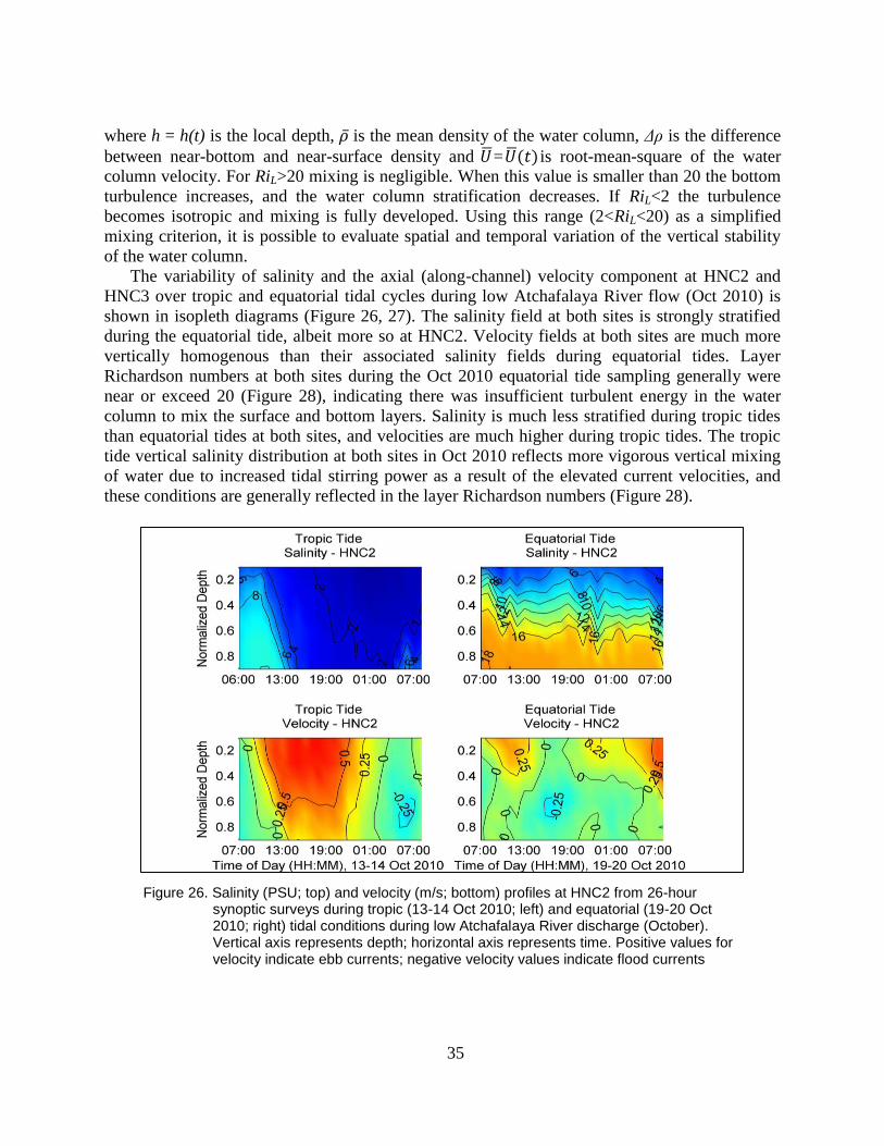
35
where h = h(t) is the local depth, is the mean density of the water column, Δρ is the difference
between near-bottom and near-surface density and = ( ) is root-mean-square of the water
column velocity. For RiL>20 mixing is negligible. When this value is smaller than 20 the bottom
turbulence increases, and the water column stratification decreases. If RiL<2 the turbulence
becomes isotropic and mixing is fully developed. Using this range (2<RiL<20) as a simplified
mixing criterion, it is possible to evaluate spatial and temporal variation of the vertical stability
of the water column.
The variability of salinity and the axial (along-channel) velocity component at HNC2 and
HNC3 over tropic and equatorial tidal cycles during low Atchafalaya River flow (Oct 2010) is
shown in isopleth diagrams (Figure 26, 27). The salinity field at both sites is strongly stratified
during the equatorial tide, albeit more so at HNC2. Velocity fields at both sites are much more
vertically homogenous than their associated salinity fields during equatorial tides. Layer
Richardson numbers at both sites during the Oct 2010 equatorial tide sampling generally were
near or exceed 20 (Figure 28), indicating there was insufficient turbulent energy in the water
column to mix the surface and bottom layers. Salinity is much less stratified during tropic tides
than equatorial tides at both sites, and velocities are much higher during tropic tides. The tropic
tide vertical salinity distribution at both sites in Oct 2010 reflects more vigorous vertical mixing
of water due to increased tidal stirring power as a result of the elevated current velocities, and
these conditions are generally reflected in the layer Richardson numbers (Figure 28).
Figure 26. Salinity (PSU; top) and velocity (m/s; bottom) profiles at HNC2 from 26-hour synoptic surveys during tropic (13-14 Oct 2010; left) and equatorial (19-20 Oct 2010; right) tidal conditions during low Atchafalaya River discharge (October). Vertical axis represents depth; horizontal axis represents time. Positive values for velocity indicate ebb currents; negative velocity values indicate flood currents
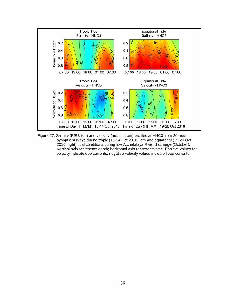
36
Figure 27. Salinity (PSU; top) and velocity (m/s; bottom) profiles at HNC3 from 26-hour synoptic surveys during tropic (13-14 Oct 2010; left) and equatorial (19-20 Oct 2010; right) tidal conditions during low Atchafalaya River discharge (October). Vertical axis represents depth; horizontal axis represents time. Positive values for velocity indicate ebb currents; negative velocity values indicate flood currents.
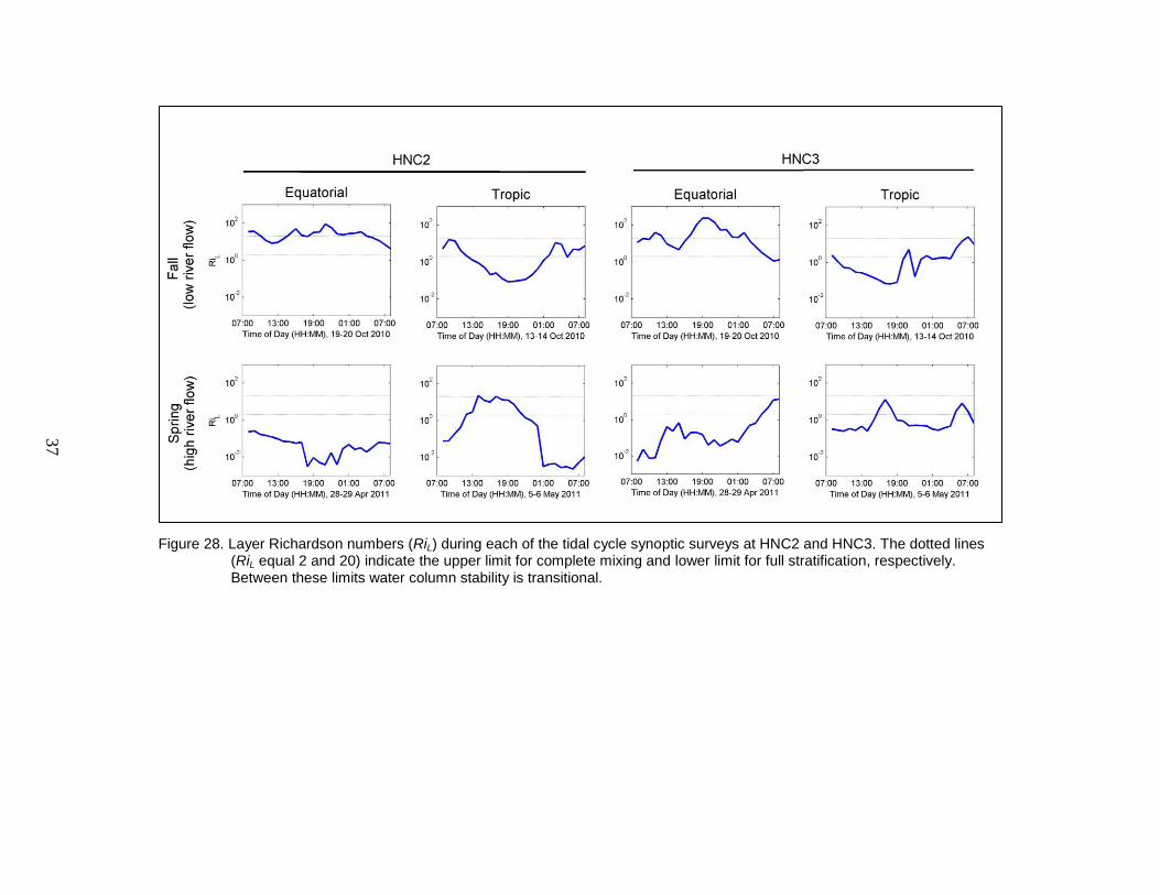
37
Figure 28. Layer Richardson numbers (RiL) during each of the tidal cycle synoptic surveys at HNC2 and HNC3. The dotted lines (RiL equal 2 and 20) indicate the upper limit for complete mixing and lower limit for full stratification, respectively. Between these limits water column stability is transitional.
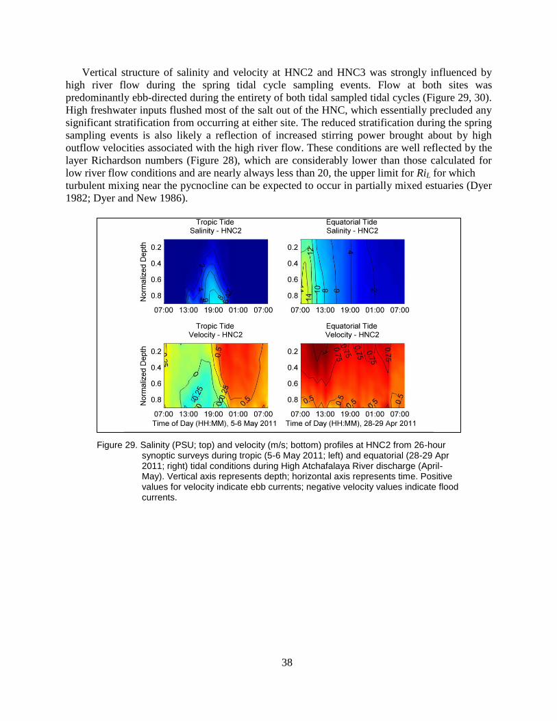
38
Vertical structure of salinity and velocity at HNC2 and HNC3 was strongly influenced by
high river flow during the spring tidal cycle sampling events. Flow at both sites was
predominantly ebb-directed during the entirety of both tidal sampled tidal cycles (Figure 29, 30).
High freshwater inputs flushed most of the salt out of the HNC, which essentially precluded any
significant stratification from occurring at either site. The reduced stratification during the spring
sampling events is also likely a reflection of increased stirring power brought about by high
outflow velocities associated with the high river flow. These conditions are well reflected by the
layer Richardson numbers (Figure 28), which are considerably lower than those calculated for
low river flow conditions and are nearly always less than 20, the upper limit for RiL for which
turbulent mixing near the pycnocline can be expected to occur in partially mixed estuaries (Dyer
1982; Dyer and New 1986).
Figure 29. Salinity (PSU; top) and velocity (m/s; bottom) profiles at HNC2 from 26-hour synoptic surveys during tropic (5-6 May 2011; left) and equatorial (28-29 Apr 2011; right) tidal conditions during High Atchafalaya River discharge (April-May). Vertical axis represents depth; horizontal axis represents time. Positive values for velocity indicate ebb currents; negative velocity values indicate flood currents.
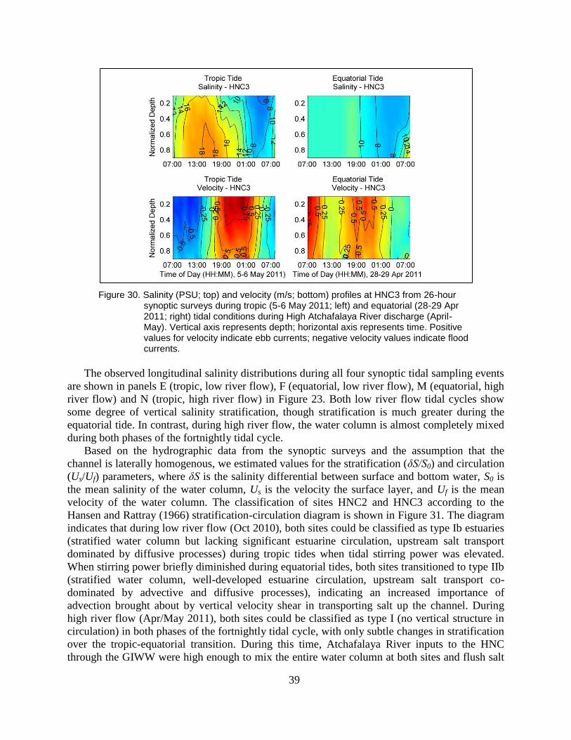
39
Figure 30. Salinity (PSU; top) and velocity (m/s; bottom) profiles at HNC3 from 26-hour synoptic surveys during tropic (5-6 May 2011; left) and equatorial (28-29 Apr 2011; right) tidal conditions during High Atchafalaya River discharge (April-May). Vertical axis represents depth; horizontal axis represents time. Positive values for velocity indicate ebb currents; negative velocity values indicate flood currents.
The observed longitudinal salinity distributions during all four synoptic tidal sampling events
are shown in panels E (tropic, low river flow), F (equatorial, low river flow), M (equatorial, high
river flow) and N (tropic, high river flow) in Figure 23. Both low river flow tidal cycles show
some degree of vertical salinity stratification, though stratification is much greater during the
equatorial tide. In contrast, during high river flow, the water column is almost completely mixed
during both phases of the fortnightly tidal cycle.
Based on the hydrographic data from the synoptic surveys and the assumption that the
channel is laterally homogenous, we estimated values for the stratification (δS/S0) and circulation
(Us/Uf) parameters, where δS is the salinity differential between surface and bottom water, S0 is
the mean salinity of the water column, Us is the velocity the surface layer, and Uf is the mean
velocity of the water column. The classification of sites HNC2 and HNC3 according to the
Hansen and Rattray (1966) stratification-circulation diagram is shown in Figure 31. The diagram
indicates that during low river flow (Oct 2010), both sites could be classified as type Ib estuaries
(stratified water column but lacking significant estuarine circulation, upstream salt transport
dominated by diffusive processes) during tropic tides when tidal stirring power was elevated.
When stirring power briefly diminished during equatorial tides, both sites transitioned to type IIb
(stratified water column, well-developed estuarine circulation, upstream salt transport co-
dominated by advective and diffusive processes), indicating an increased importance of
advection brought about by vertical velocity shear in transporting salt up the channel. During
high river flow (Apr/May 2011), both sites could be classified as type I (no vertical structure in
circulation) in both phases of the fortnightly tidal cycle, with only subtle changes in stratification
over the tropic-equatorial transition. During this time, Atchafalaya River inputs to the HNC
through the GIWW were high enough to mix the entire water column at both sites and flush salt
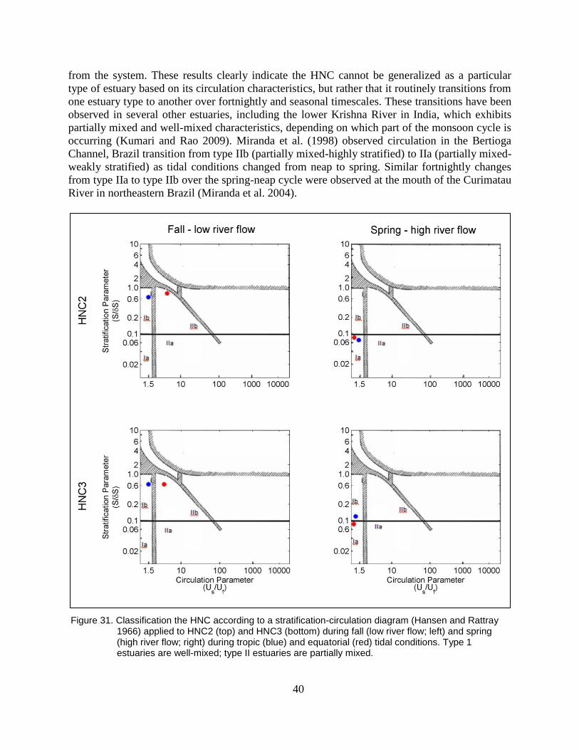
40
from the system. These results clearly indicate the HNC cannot be generalized as a particular
type of estuary based on its circulation characteristics, but rather that it routinely transitions from
one estuary type to another over fortnightly and seasonal timescales. These transitions have been
observed in several other estuaries, including the lower Krishna River in India, which exhibits
partially mixed and well-mixed characteristics, depending on which part of the monsoon cycle is
occurring (Kumari and Rao 2009). Miranda et al. (1998) observed circulation in the Bertioga
Channel, Brazil transition from type IIb (partially mixed-highly stratified) to IIa (partially mixed-
weakly stratified) as tidal conditions changed from neap to spring. Similar fortnightly changes
from type IIa to type IIb over the spring-neap cycle were observed at the mouth of the Curimatau
River in northeastern Brazil (Miranda et al. 2004).
Figure 31. Classification the HNC according to a stratification-circulation diagram (Hansen and Rattray 1966) applied to HNC2 (top) and HNC3 (bottom) during fall (low river flow; left) and spring (high river flow; right) during tropic (blue) and equatorial (red) tidal conditions. Type 1 estuaries are well-mixed; type II estuaries are partially mixed.
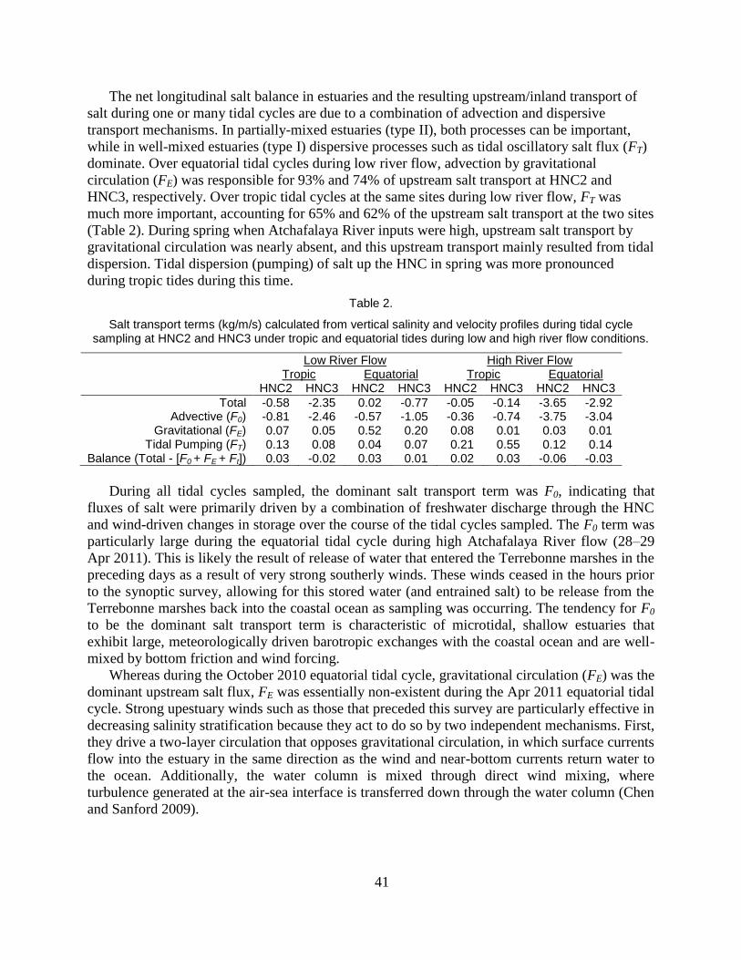
41
The net longitudinal salt balance in estuaries and the resulting upstream/inland transport of
salt during one or many tidal cycles are due to a combination of advection and dispersive
transport mechanisms. In partially-mixed estuaries (type II), both processes can be important,
while in well-mixed estuaries (type I) dispersive processes such as tidal oscillatory salt flux (FT)
dominate. Over equatorial tidal cycles during low river flow, advection by gravitational
circulation (FE) was responsible for 93% and 74% of upstream salt transport at HNC2 and
HNC3, respectively. Over tropic tidal cycles at the same sites during low river flow, FT was
much more important, accounting for 65% and 62% of the upstream salt transport at the two sites
(Table 2). During spring when Atchafalaya River inputs were high, upstream salt transport by
gravitational circulation was nearly absent, and this upstream transport mainly resulted from tidal
dispersion. Tidal dispersion (pumping) of salt up the HNC in spring was more pronounced
during tropic tides during this time.
Table 2.
Salt transport terms (kg/m/s) calculated from vertical salinity and velocity profiles during tidal cycle sampling at HNC2 and HNC3 under tropic and equatorial tides during low and high river flow conditions.
Low River Flow High River Flow Tropic Equatorial Tropic Equatorial HNC2 HNC3 HNC2 HNC3 HNC2 HNC3 HNC2 HNC3
Total -0.58 -2.35 0.02 -0.77 -0.05 -0.14 -3.65 -2.92 Advective (F0) -0.81 -2.46 -0.57 -1.05 -0.36 -0.74 -3.75 -3.04
Gravitational (FE) 0.07 0.05 0.52 0.20 0.08 0.01 0.03 0.01 Tidal Pumping (FT) 0.13 0.08 0.04 0.07 0.21 0.55 0.12 0.14
Balance (Total - [F0 + FE + Ft]) 0.03 -0.02 0.03 0.01 0.02 0.03 -0.06 -0.03
During all tidal cycles sampled, the dominant salt transport term was F0, indicating that
fluxes of salt were primarily driven by a combination of freshwater discharge through the HNC
and wind-driven changes in storage over the course of the tidal cycles sampled. The F0 term was
particularly large during the equatorial tidal cycle during high Atchafalaya River flow (28–29
Apr 2011). This is likely the result of release of water that entered the Terrebonne marshes in the
preceding days as a result of very strong southerly winds. These winds ceased in the hours prior
to the synoptic survey, allowing for this stored water (and entrained salt) to be release from the
Terrebonne marshes back into the coastal ocean as sampling was occurring. The tendency for F0
to be the dominant salt transport term is characteristic of microtidal, shallow estuaries that
exhibit large, meteorologically driven barotropic exchanges with the coastal ocean and are well-
mixed by bottom friction and wind forcing.
Whereas during the October 2010 equatorial tidal cycle, gravitational circulation (FE) was the
dominant upstream salt flux, FE was essentially non-existent during the Apr 2011 equatorial tidal
cycle. Strong upestuary winds such as those that preceded this survey are particularly effective in
decreasing salinity stratification because they act to do so by two independent mechanisms. First,
they drive a two-layer circulation that opposes gravitational circulation, in which surface currents
flow into the estuary in the same direction as the wind and near-bottom currents return water to
the ocean. Additionally, the water column is mixed through direct wind mixing, where
turbulence generated at the air-sea interface is transferred down through the water column (Chen
and Sanford 2009).
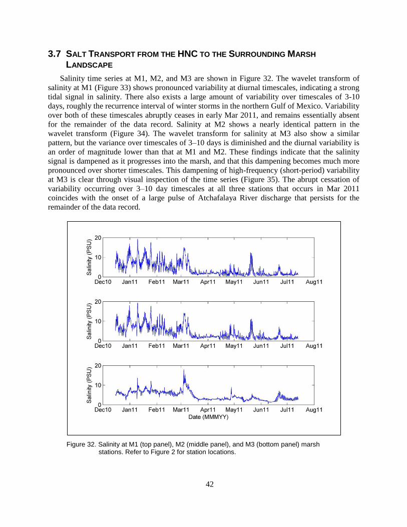
42
3.7 SALT TRANSPORT FROM THE HNC TO THE SURROUNDING MARSH
LANDSCAPE
Salinity time series at M1, M2, and M3 are shown in Figure 32. The wavelet transform of
salinity at M1 (Figure 33) shows pronounced variability at diurnal timescales, indicating a strong
tidal signal in salinity. There also exists a large amount of variability over timescales of 3-10
days, roughly the recurrence interval of winter storms in the northern Gulf of Mexico. Variability
over both of these timescales abruptly ceases in early Mar 2011, and remains essentially absent
for the remainder of the data record. Salinity at M2 shows a nearly identical pattern in the
wavelet transform (Figure 34). The wavelet transform for salinity at M3 also show a similar
pattern, but the variance over timescales of 3–10 days is diminished and the diurnal variability is
an order of magnitude lower than that at M1 and M2. These findings indicate that the salinity
signal is dampened as it progresses into the marsh, and that this dampening becomes much more
pronounced over shorter timescales. This dampening of high-frequency (short-period) variability
at M3 is clear through visual inspection of the time series (Figure 35). The abrupt cessation of
variability occurring over 3–10 day timescales at all three stations that occurs in Mar 2011
coincides with the onset of a large pulse of Atchafalaya River discharge that persists for the
remainder of the data record.
Figure 32. Salinity at M1 (top panel), M2 (middle panel), and M3 (bottom panel) marsh stations. Refer to Figure 2 for station locations.
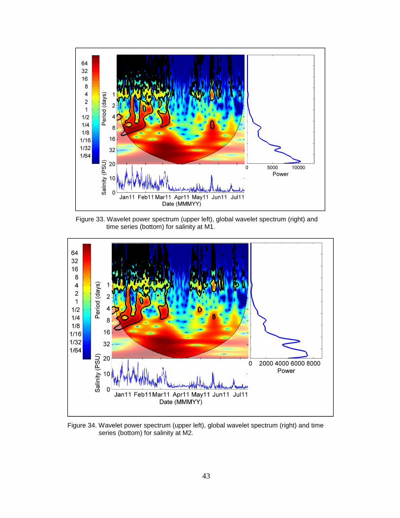
43
Figure 33. Wavelet power spectrum (upper left), global wavelet spectrum (right) and time series (bottom) for salinity at M1.
Figure 34. Wavelet power spectrum (upper left), global wavelet spectrum (right) and time series (bottom) for salinity at M2.
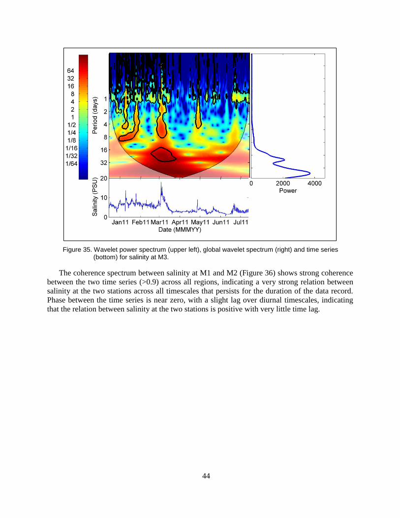
44
Figure 35. Wavelet power spectrum (upper left), global wavelet spectrum (right) and time series (bottom) for salinity at M3.
The coherence spectrum between salinity at M1 and M2 (Figure 36) shows strong coherence
between the two time series (>0.9) across all regions, indicating a very strong relation between
salinity at the two stations across all timescales that persists for the duration of the data record.
Phase between the time series is near zero, with a slight lag over diurnal timescales, indicating
that the relation between salinity at the two stations is positive with very little time lag.
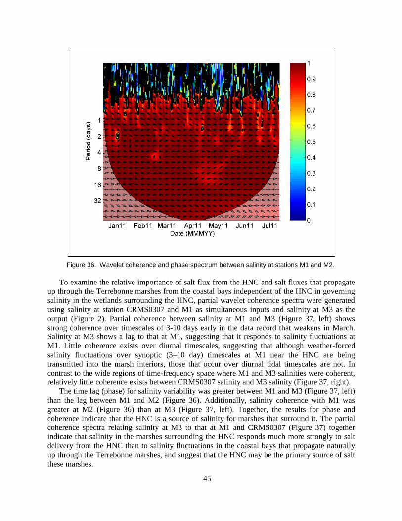
45
Figure 36. Wavelet coherence and phase spectrum between salinity at stations M1 and M2.
To examine the relative importance of salt flux from the HNC and salt fluxes that propagate
up through the Terrebonne marshes from the coastal bays independent of the HNC in governing
salinity in the wetlands surrounding the HNC, partial wavelet coherence spectra were generated
using salinity at station CRMS0307 and M1 as simultaneous inputs and salinity at M3 as the
output (Figure 2). Partial coherence between salinity at M1 and M3 (Figure 37, left) shows
strong coherence over timescales of 3-10 days early in the data record that weakens in March.
Salinity at M3 shows a lag to that at M1, suggesting that it responds to salinity fluctuations at
M1. Little coherence exists over diurnal timescales, suggesting that although weather-forced
salinity fluctuations over synoptic (3–10 day) timescales at M1 near the HNC are being
transmitted into the marsh interiors, those that occur over diurnal tidal timescales are not. In
contrast to the wide regions of time-frequency space where M1 and M3 salinities were coherent,
relatively little coherence exists between CRMS0307 salinity and M3 salinity (Figure 37, right).
The time lag (phase) for salinity variability was greater between M1 and M3 (Figure 37, left)
than the lag between M1 and M2 (Figure 36). Additionally, salinity coherence with M1 was
greater at M2 (Figure 36) than at M3 (Figure 37, left). Together, the results for phase and
coherence indicate that the HNC is a source of salinity for marshes that surround it. The partial
coherence spectra relating salinity at M3 to that at M1 and CRMS0307 (Figure 37) together
indicate that salinity in the marshes surrounding the HNC responds much more strongly to salt
delivery from the HNC than to salinity fluctuations in the coastal bays that propagate naturally
up through the Terrebonne marshes, and suggest that the HNC may be the primary source of salt
these marshes.
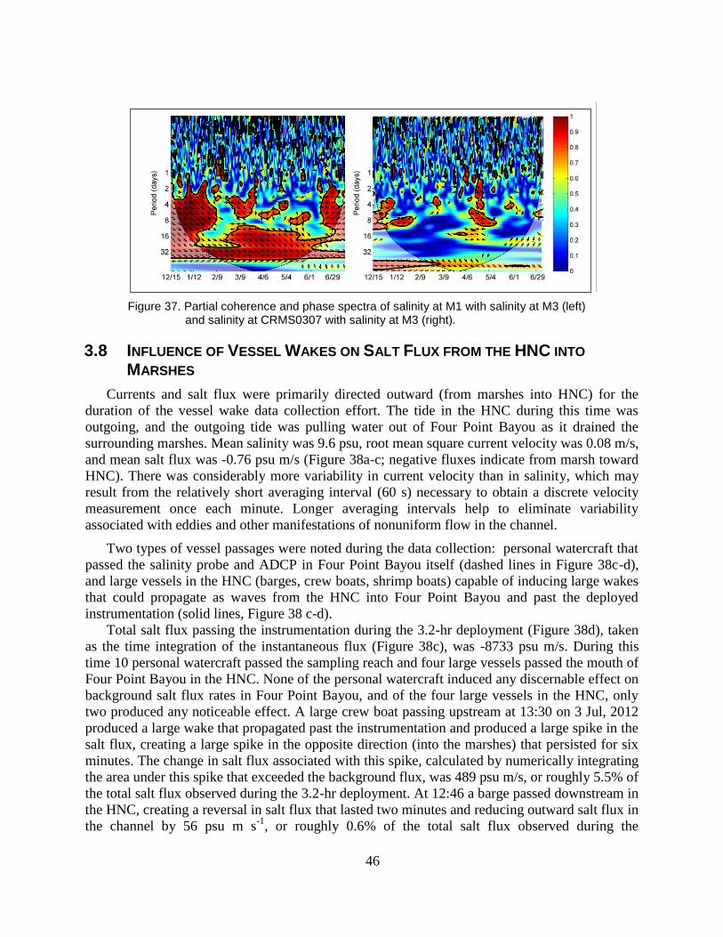
46
Figure 37. Partial coherence and phase spectra of salinity at M1 with salinity at M3 (left) and salinity at CRMS0307 with salinity at M3 (right).
3.8 INFLUENCE OF VESSEL WAKES ON SALT FLUX FROM THE HNC INTO
MARSHES
Currents and salt flux were primarily directed outward (from marshes into HNC) for the
duration of the vessel wake data collection effort. The tide in the HNC during this time was
outgoing, and the outgoing tide was pulling water out of Four Point Bayou as it drained the
surrounding marshes. Mean salinity was 9.6 psu, root mean square current velocity was 0.08 m/s,
and mean salt flux was -0.76 psu m/s (Figure 38a-c; negative fluxes indicate from marsh toward
HNC). There was considerably more variability in current velocity than in salinity, which may
result from the relatively short averaging interval (60 s) necessary to obtain a discrete velocity
measurement once each minute. Longer averaging intervals help to eliminate variability
associated with eddies and other manifestations of nonuniform flow in the channel.
Two types of vessel passages were noted during the data collection: personal watercraft that
passed the salinity probe and ADCP in Four Point Bayou itself (dashed lines in Figure 38c-d),
and large vessels in the HNC (barges, crew boats, shrimp boats) capable of inducing large wakes
that could propagate as waves from the HNC into Four Point Bayou and past the deployed
instrumentation (solid lines, Figure 38 c-d).
Total salt flux passing the instrumentation during the 3.2-hr deployment (Figure 38d), taken
as the time integration of the instantaneous flux (Figure 38c), was -8733 psu m/s. During this
time 10 personal watercraft passed the sampling reach and four large vessels passed the mouth of
Four Point Bayou in the HNC. None of the personal watercraft induced any discernable effect on
background salt flux rates in Four Point Bayou, and of the four large vessels in the HNC, only
two produced any noticeable effect. A large crew boat passing upstream at 13:30 on 3 Jul, 2012
produced a large wake that propagated past the instrumentation and produced a large spike in the
salt flux, creating a large spike in the opposite direction (into the marshes) that persisted for six
minutes. The change in salt flux associated with this spike, calculated by numerically integrating
the area under this spike that exceeded the background flux, was 489 psu m/s, or roughly 5.5% of
the total salt flux observed during the 3.2-hr deployment. At 12:46 a barge passed downstream in
the HNC, creating a reversal in salt flux that lasted two minutes and reducing outward salt flux in
the channel by 56 psu m s-1
, or roughly 0.6% of the total salt flux observed during the
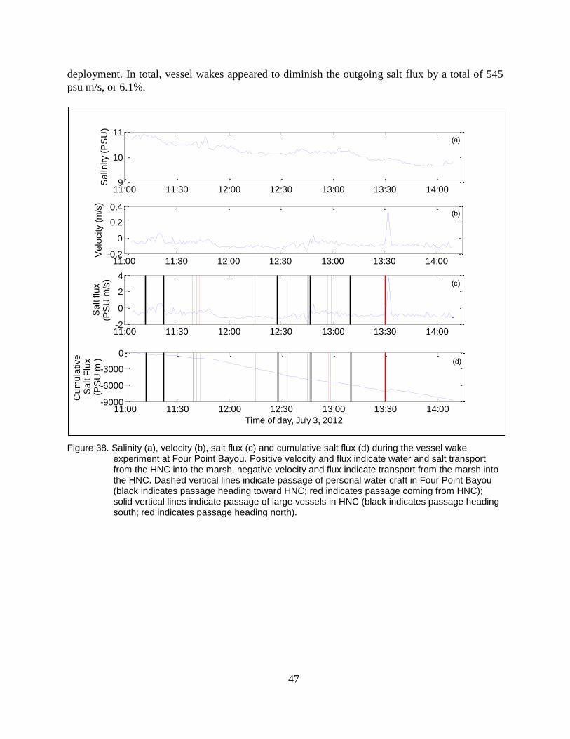
47
deployment. In total, vessel wakes appeared to diminish the outgoing salt flux by a total of 545
psu m/s, or 6.1%.
Figure 38. Salinity (a), velocity (b), salt flux (c) and cumulative salt flux (d) during the vessel wake experiment at Four Point Bayou. Positive velocity and flux indicate water and salt transport from the HNC into the marsh, negative velocity and flux indicate transport from the marsh into the HNC. Dashed vertical lines indicate passage of personal water craft in Four Point Bayou (black indicates passage heading toward HNC; red indicates passage coming from HNC); solid vertical lines indicate passage of large vessels in HNC (black indicates passage heading south; red indicates passage heading north).
11:00 11:30 12:00 12:30 13:00 13:30 14:009
10
11
Sa
lin
ity (
PS
U)
11:00 11:30 12:00 12:30 13:00 13:30 14:00-0.2
0
0.2
0.4
Ve
locity (
m/s
)
11:00 11:30 12:00 12:30 13:00 13:30 14:00-2
0
2
4
Sa
lt flu
x(P
SU
m/s
)
11:00 11:30 12:00 12:30 13:00 13:30 14:00-9000
-6000
-3000
0
Time of day, July 3, 2012
Cu
mu
lative
S
alt F
lux
(PS
U m
)
(a)
(b)
(c)
(d)

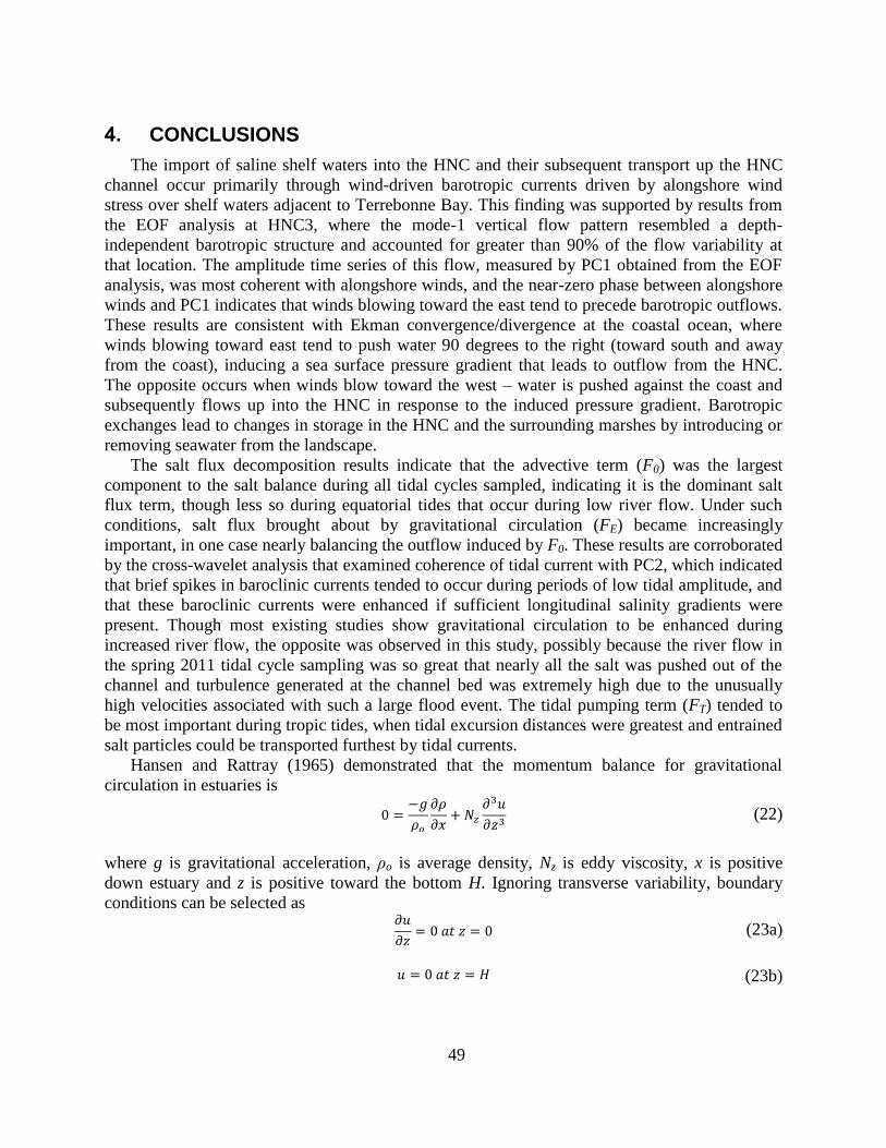
49
4. CONCLUSIONS
The import of saline shelf waters into the HNC and their subsequent transport up the HNC
channel occur primarily through wind-driven barotropic currents driven by alongshore wind
stress over shelf waters adjacent to Terrebonne Bay. This finding was supported by results from
the EOF analysis at HNC3, where the mode-1 vertical flow pattern resembled a depth-
independent barotropic structure and accounted for greater than 90% of the flow variability at
that location. The amplitude time series of this flow, measured by PC1 obtained from the EOF
analysis, was most coherent with alongshore winds, and the near-zero phase between alongshore
winds and PC1 indicates that winds blowing toward the east tend to precede barotropic outflows.
These results are consistent with Ekman convergence/divergence at the coastal ocean, where
winds blowing toward east tend to push water 90 degrees to the right (toward south and away
from the coast), inducing a sea surface pressure gradient that leads to outflow from the HNC.
The opposite occurs when winds blow toward the west – water is pushed against the coast and
subsequently flows up into the HNC in response to the induced pressure gradient. Barotropic
exchanges lead to changes in storage in the HNC and the surrounding marshes by introducing or
removing seawater from the landscape.
The salt flux decomposition results indicate that the advective term (F0) was the largest
component to the salt balance during all tidal cycles sampled, indicating it is the dominant salt
flux term, though less so during equatorial tides that occur during low river flow. Under such
conditions, salt flux brought about by gravitational circulation (FE) became increasingly
important, in one case nearly balancing the outflow induced by F0. These results are corroborated
by the cross-wavelet analysis that examined coherence of tidal current with PC2, which indicated
that brief spikes in baroclinic currents tended to occur during periods of low tidal amplitude, and
that these baroclinic currents were enhanced if sufficient longitudinal salinity gradients were
present. Though most existing studies show gravitational circulation to be enhanced during
increased river flow, the opposite was observed in this study, possibly because the river flow in
the spring 2011 tidal cycle sampling was so great that nearly all the salt was pushed out of the
channel and turbulence generated at the channel bed was extremely high due to the unusually
high velocities associated with such a large flood event. The tidal pumping term (FT) tended to
be most important during tropic tides, when tidal excursion distances were greatest and entrained
salt particles could be transported furthest by tidal currents.
Hansen and Rattray (1965) demonstrated that the momentum balance for gravitational
circulation in estuaries is
(22)
where g is gravitational acceleration, ρo is average density, Nz is eddy viscosity, x is positive
down estuary and z is positive toward the bottom H. Ignoring transverse variability, boundary
conditions can be selected as
(23a)
(23b)
50
∫
(23c)
Equation (23a) indicates no wind stress-induced velocity shear exists at the water surface,
(23b) declares a no-slip condition exists at the bottom, and (23c) represents continuity with the
assumption that river discharge is much smaller than the volume flux associated with
gravitational circulation. The solution of (22), subject to (23a-c), was provided by Officer (1976)
as
( )
[ (
)
(
)
] (24)
Using the density difference between Terrebonne Bay and HNC2 at the time of the two fall
(13–14 Oct 2010, 19–20 Oct 2010) tidal-cycle surveys to estimate
and the values of RiL
calculated from those surveys to estimate Nz (5.4 x 10⁻⁴
m2/s for equatorial tides; 2.3 x 10
-3 m
2/s
for tropic tides; Bowden and Hamilton 1975), equation (18) can be used to estimate the depth-
specific velocity associated with gravitational circulation (Figure 39). Currently the HNC
channel is maintained to a depth of 4.57m (15 ft), but proposals to deepen the channel depth to
6.1 m have been investigated (U.S. Army Corps of Engineers 2003). The velocities predicted by
(24) for the current channel configuration closely reflect the magnitudes of the baroclinic
component extracted from the current meter time series at HNC3 with EOF analysis (Figure 8).
By deepening the channel to 6.1m, one could expect to observe over three times the landward
transport below the pycnocline that occurs under the current channel configuration. Presumably
this enhanced landward transport would enhance salt flux up the channel and may enhance water
column salinity stratification. Wang (1988) used a laterally-averaged, semi-implicit
hydrodynamic model to predict a 25-km inland migration of the 5 psu isohaline associated with
doubling the maintained depth of the HNC.
51
Figure 39. Depth-specific current velocity associated with gravitational circulation as predicted by Officer
(1976; Equation 18) during tropic (left) and equatorial (right) tidal conditions under low river flow. Current channel configuration (H = 4.5 m) shown by blue line, deepened configuration (H = 6.1 m) shown by red line. Positive values indicate ebb-directed currents.
Results from the 19 salinity transects indicate that the along-channel salinity structure in the
HNC can vary widely, both in terms of vertical (salt wedge) structure and in terms of saltwater
intrusion length. The multiple regression analysis indicated that this length is mainly governed
by Atchafalaya River discharge, but also by alongshore wind stress. Signs of regression
coefficients indicate that increased river flows decrease saltwater intrusion length, and that wind
stress toward the east can further reduce it. Together, these two variables explained nearly 85%
of the observed variability in saltwater intrusion length. Vertical salinity stratification, observed
both through the salinity transects and the time series salinity data obtained at HNC2, responded
strongly to variations in tidal stirring power over the course of the tropic-equatorial cycle. The
temporal resolution provided by the time series data at HNC2 showed that in addition to
fortnightly cycles in salinity stratification, there were times when the water column also went
through stratification-destratification cycles over the course of a tidal cycle, where it tended to
stratify at the end of the ebb tide, and rapidly destratify after the tide reversed and began to flow
upestuary.
52
Cross-wavelet analyses indicate that the HNC may be the primary source of salt for marshes
in the surrounding landscape. Salinity at M3 responded much more strongly to salinity at M1,
which has an immediate connection with the HNC, than it did to CRMS0307, situated near the
seaward extent of the Terrebonne marshes. This finding was further supported by the fact that the
phase between M1 and M3 salinity was greater than that between M1 and M2, suggesting that
salt in the HNC propagates into the marsh, passing M1 and M2 before reaching M3. These
results suggest that salt is much more efficiently transported to the Terrebonne marshes via the
HNC than it would be through natural pathways through the marshes of the lower basin.
Finally, the effect of vessel wakes on the delivery of salt from the HNC into the surrounding
marshes appears to be minimal. During an outgoing tide, influxes associated with vessel wakes
appeared to diminish the outgoing salt flux by roughly 6%. It is quite possible that this 6% was
eventually released during the outgoing tide, but there is no way to determine if this release did
or did not occur. Compared to energetic inflows of salt water from the HNC into surrounding
marshes driven by weather and tidal pumping, it seems likely that brief wake-related flows
lasting on the order of two minutes have relatively little impact on salt delivery to these
landscapes.
53
LITERATURE CITED
Bendat, J.S. and A.G. Piersol. 1986. Random Data: Analysis and Measurement Procedures. John
Wiley and Sons, NY. 566 pp.
Bloomfield, P. 1976. Fourier Analysis of Time Series: An Introduction. John Wiley, New York.
432 pp.
Boon, J.D. 2004. Secrets of the Tide: Tide and Tidal Current Analysis and Applications, Storm
Surges and Sea Level Trends. Woodhead Publishing, NY. 224 pp.
Bowden, K.F. and P. Hamilton. 1975. Some experiments with a numerical model of circulation
and mixing in a tidal estuary. Estuarine, Coastal and Marine Science 3:281-301.
Chabreck, R.H., T. Joanen, and A.W. Palmisano. 1968. Vegetation type map of the Louisiana
coastal marshes:Louisiana Cooperative Wildlife Research Unit, Louisiana Wildlife and
Fisheries Commission, and Louisiana State University, 1 sheet, scale 1:100,000.
Chabreck, R.H., and R.G. Linscombe. 1978. Vegetative type map of the Louisiana coastal
marshes: Baton Rouge, LA., Louisiana Department of Wildlife and Fisheries, 1 sheet, scale
1:100,000.
Chabreck, R.H., and R.G. Linscombe. 1988, Vegetative type map of the Louisiana coastal
marshes: Baton Rouge, LA., Louisiana Department of Wildlife and Fisheries, 1 sheet, scale
1:100,000.
Chabreck, R.H., and R.G. Linscombe. 1997. Louisiana coastal marsh vegetative type map: Baton
Rouge, LA., Louisiana State University and Louisiana Department of Wildlife and Fisheries,
1 sheet, scale not given.
Chen, S.N., and L.P. Sanford. 2009. Axial wind effects on stratification and longitudinal salt
transport in an idealized, partially mixed estuary. Journal of Physical Oceanography 39:1905-
1920.
Chuang, W.S. and W.J. Wiseman. 1983. Coastal sea level response to frontal passages on the
Louisiana-Texas shelf. Journal of Geophysical Research 88:2615-2620.
Couvillion, B.R., J.A. Barras, G.D. Steyer, W. Sleavin, M. Fischer, H. Beck, N. Trahan, B.
Griffin, and D. Heckman. 2011. Land area change in coastal Louisiana from 1932 to 2010.
U.S. Geological Survey Scientific Investigations Map 3164.
Daubechies, I. 1990. The wavelet transform, time-frequency localization and signal analysis.
IEEE Transactions – Information Theory 36:961-1005.
54
Dronkers, J.J. 1964. Tidal Computations in Rivers and Coastal Waters. North Holland
Publishing, Amsterdam. 518 pp.
Dyer, K.R. 1973. Estuaries: A Physical Introduction. John Wiley and Sons, New York. 195 pp.
Dyer, K.R. 1982. Mixing caused by lateral internal seiching within a partially mixed estuary.
Estuarine, Coastal and Shelf Science 15:443-457.
Dyer, K.R., and A.L. New. 1986. Intermittency in Estuarine Mixing. Academic Press, New
York.
Elliott, A.J. and D.P. Wang. 1978. The effect of meteorological forcing on the Chesapeake Bay:
the coupling between and estuarine system and its adjacent coastal waters. In:
Hydrodynamics of Estuaries and Fjords (ed. J.C.J. Nihoul), Elsvier Scientific Pulb. Co.,
Amsterdam, pp 127-145.
Epifanio, C.E. 1995. Transport of blue crab (Callinectes sapidus) larvae in the waters off Mid-
Atlantic states. Bulletin of Marine Science 57:713-725.
Garrett, C., and B. Toulany 1982. Sea level variability due to meteorological forcing in the
northwest Gulf of St. Lawrence. Journal of Geophysical Research 87:1968-1978.
Geyer, W.R. 1995. Tide-induced mixing in the Amazon frontal zone. Journal of Geophysical
Research 100:2341-2353.
Geyer, W.R. and G.A. Cannon. 1982. Sill processes related to deep water renewal in a Fjord.
Journal of Geophysical Research 87:7985-7996.
Geyer, W.R., and R.P. Signell. 1992. A reassessment of the role of tidal dispersion in estuaries
and bays. Estuaries 15: 97-108.
Geyer R.W. and J.D. Smith. 1987. Shear instability in a highly stratified estuary. Journal of
Physical Oceanography 19:1060-1072
Geyer, W.R., J.H. Trowbridge, and M. Bowen, 2000. The dynamics of a partially mixed estuary.
Journal of Physical Oceanography 30: 2035-2048.
Griffin, D.A. and P.H. Leblond. 1990. Estuary-ocean exchange controlled by spring-neap tidal
mixing. Estuarine, Coastal and Shelf Science 30: 275-297.
Hansen, D.V. and M. Rattray. 1965. Gravitational circulation in straits and estuaries. Journal of
Marine Research 23:104-122.
55
Hansen, D.V. and M. Rattray. 1966. New dimensions in estuary classification. Limnology and
Oceanography 11: 319-326.
Horn, D.A., B. Laval, J. Imberger, and A.N. Findikakas. 2001. Field study of physical processes
in Lake Maracaibo, in Proceedings XXIX IAHR Congress, Beijing, China.
Janzen, C.D. and K.C. Wong. 2002. Wind-forced dynamics at the estuary-shelf interface of a
large coastal plain estuary. Journal of Geophysical Research 107 (C10), 3138,
doi:10.1029/2001JC000959.
Jevrejeva, S., J.C. Moore, and A. Grinsted. 2003. Influence of the Arctic oscillation and El Nino-
southern oscillation (ENSO) on ice conditions in the Baltic Sea: the wavelet approach.
Journal of Geophysical Research 108: 4677.
Jevrejeva, S., J.C. Moore, P.L. Woodworth, and A. Grinsted. 2005. Influence of large-scale
atmospheric circulation on European sea level: results based on the wavelet transform
method. Tellus 57: 183-193.
Kayano, M.T. and R.V. Andreoli. 2006. Relationships between rainfall anomalies over
northeastern Brazil and El Nino-Southern Oscillation. Journal of Geophysical Research
111:D13101.
Kjerfve, B. 1975. Velocity average in estuaries characterized by a large tidal range to depth ratio.
Estuarine and Coastal Marine Science 3:311-324.
Kjerfve, B. 1986. Circulation and salt flux in a well-mixed estuary. pp. 22-29 in Van de Kreeke,
J. (ed.). Physics of Shallow Estuaries and Bays. Springer Verlag, Berlin. 280 pp.
Kumari, V.R. and I.M. Rao. 2009. Estuarine characteristics of lower Krishna river. Indian
Journal of Marine Sciences 38:215-223.
Labat, D., Y. Godderis, J.L. Probst, and J.L. Guyot. 2004. Evidence for global runoff increase
related to climate warming. Advances in Water Resources 27: 631-642.
Linscombe, G., R.H. Chabreck, and S. Hartley. 2001. Aerial mapping of marsh dieback in saline
marshes in the Barataria - Terrebonne Basins [abs.]: Abstracts from “Coastal Marsh Dieback
in the Northern Gulf of Mexico: Extent, Causes, Consequences, and Remedies,” USGS
Information and Technology Report, USGS/BRD/ITR-2001-0003, 31 pp.
MacCready, P. 1999. Estuarine adjustment to changes in river flow and tidal mixing. Journal of
Physical Oceanography 29:708-726.
MacCready, P. 2004. Toward a unified theory of tidally-averaged estuarine salinity structure.
Estuaries 27:561-570.
56
MacCready, P. 2007. Estuarine adjustment. Journal of Physical Oceanography 37:2133-2145.
Medeiros, C., and B. Kjerfve. 2005. Longitudinal salt and sediment fluxes in a tropical estuary:
Itamaraca, Brazil. Journal of Coastal Research 21:751:758.
Miranda, L.B., A.L. Bergamo, and B.M. Castro. 2005. Interactions of river discharge and tidal
modulation in a tropical estuary, NE Brazil. Ocean Dynamics 55:430-440.
Miranda, L.B., A.L. Bergamo, and C.A. Ramos e Silva. 2004. Dynamics of a tropical estuary:
Curimatau River, NE Brazil. Journal of Coastal Research Special Issue 39: 697-701.
Miranda, L.B., B.M. Castro, and B.J. Kjerfve. 1998. Circulation and mixing due to tidal forcing
in the Bertioga Channel, Sao Paulo, Brazil. Estuaries 21:204-214.
Monismith, S.G. and D.A. Fong. 1996. A simple model of mixing in stratified tidal flows.
Journal of Geophysical Research 102:28583-28595.
Nunes, R.A. and G.W. Lennon. 1987. Episodic stratification and gravity currents in a marine
environment of modulated turbulence. Journal of Geophysical Research 92:5465-5480.
Officer, C.B. 1976. Physical Oceanography of Estuaries and Associated Coastal Waters. John
Wiley and Sons, New York. 465 pp.
Peters, H. 1997. Observations of stratified turbulent mixing in an estuary: neap-to-spring
variations during high river flow. Estuarine, Coastal and Shelf Science 45:69-88.
Pond, S. and G.L. Pickard. 1983. Introductory Dynamical Oceanography, 2nd edition.
Butterworth-Heinemann, Oxford, UK. 329 pp.
Preisendorfer, R.W. 1988. Principal Component Analysis in Meteorology and Oceanography.
Elsvier, Amsterdam. 425 pp.
Ribeiro, C.H.A., J.J. Waniek, and J. Sharples. 2004. Observations of the spring-neap modulation
of the gravitational circulation in a partially mixed estuary. Ocean Dynamics 54:299-306.
Simpson, J.H., J. Brown, J. Matthews, and G. Allen. 1990. Tidal straining, density currents, and
stirring in the control of estuarine stratification. Estuaries 13:125-132.
Snedden, G.A. 2006. River, tidal and wind interactions in a deltaic estuarine system. Ph.D.
dissertation, Louisiana State University, Baton Rouge, LA, USA. 116 pp.
57
Snedden, G.A., J.E. Cable, and B.J. Kjerfve. 2013. Estuarine geomorphology and hydrology, in
Day, J.W., B.C. Crump, W.M. Kemp, and A. Yanez-Arancibia, (ed.). Estuarine Ecology, 2nd
edition. Wiley-Blackwell, Hoboken, NJ, USA. pp. 19-38.
Snedden, G.A., J.E. Cable, and W.J. Wiseman, Jr. 2007. Subtidal sea level variability in a
Mississippi River deltaic estuary. Estuaries and Coasts 30:802-812.
Steyer, G.D., C. Sasser, E. Evers, E. Swenson, G. Suir, and S. Sapkota. 2008. Influence of the
Houma Navigation Canal on Salinity Patterns and Landscape Configuration in Coastal
Louisiana. U.S. Geological Survey Open-File Report 2008-1127. 190 pp.
Swarzenski, C.M. 2003. Surface-water hydrology of the Gulf Intracoastal Waterway in South-
Central Louisiana, 1996-1999. U.S. Geological Survey professional paper 1672. 51 pp.
Torrence, C. and P. Webster. 1999. Interdecadal changes in the ENSO-monsoon system. Journal
of Climate 12:2679-2690.
Turner, R.E. 1997. Wetland loss in the northern Gulf of Mexico: multiple working hypotheses.
Estuaries 20:1-13.
U.S. Army Corps of Engineers. 2003. Houma Navigation Canal, Louisiana general re-evaluation
study, channel deepening model study report. U.S. Army Corps of Engineers, New Orleans
District.
Wang, D.P. 1979. Subtidal sea level variations in the Chesapeake Bay and relations to
atmospheric forcing. Journal of Physical oceanography 9: 413-421.
Wang, F.C. 1988. Dynamics of saltwater intrusion in coastal channels. Journal of Geophysical
Research 93: 6937-6946.
Wong, K.C. 1990. Sea level variability in Long Island Sound. Estuaries 13:362-372.
Wong, K.C. 2002. On the wind-induced exchange between Indian River Bay, Delaware, and the
adjacent continental shelf. Continental Shelf Research 22: 1651-1668.
Wong, K.C. and R.W. Garvine. 1984. Observations of wind-induced, subtidal variability in the
Delaware Estuary. Journal of Geophysical Research 89:589-597.
Wong, K.C and J.E. Moses-Hall. 1988. On the relative importance of the remote and local wind
effects to the subtidal variability in a coastal plain estuary. Journal of Geophysical Research
89:18393-18404.


APPENDIX

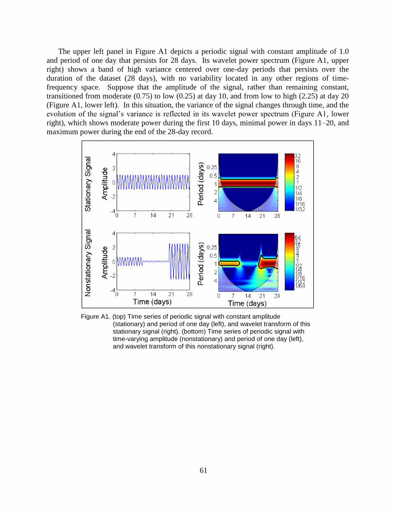
61
The upper left panel in Figure A1 depicts a periodic signal with constant amplitude of 1.0
and period of one day that persists for 28 days. Its wavelet power spectrum (Figure A1, upper
right) shows a band of high variance centered over one-day periods that persists over the
duration of the dataset (28 days), with no variability located in any other regions of time-
frequency space. Suppose that the amplitude of the signal, rather than remaining constant,
transitioned from moderate (0.75) to low (0.25) at day 10, and from low to high (2.25) at day 20
(Figure A1, lower left). In this situation, the variance of the signal changes through time, and the
evolution of the signal’s variance is reflected in its wavelet power spectrum (Figure A1, lower
right), which shows moderate power during the first 10 days, minimal power in days 11–20, and
maximum power during the end of the 28-day record.
Figure A1. (top) Time series of periodic signal with constant amplitude (stationary) and period of one day (left), and wavelet transform of this stationary signal (right). (bottom) Time series of periodic signal with time-varying amplitude (nonstationary) and period of one day (left), and wavelet transform of this nonstationary signal (right).
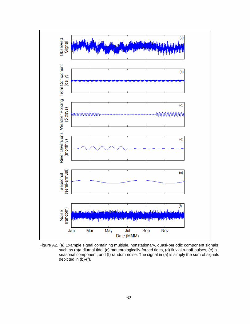
62
Figure A2. (a) Example signal containing multiple, nonstationary, quasi-periodic component signals such as (b)a diurnal tide, (c) meteorologically-forced tides, (d) fluvial runoff pulses, (e) a seasonal component, and (f) random noise. The signal in (a) is simply the sum of signals depicted in (b)-(f).
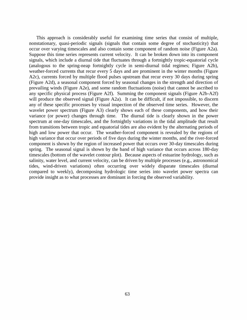
63
This approach is considerably useful for examining time series that consist of multiple,
nonstationary, quasi-periodic signals (signals that contain some degree of stochasticity) that
occur over varying timescales and also contain some component of random noise (Figure A2a).
Suppose this time series represents current velocity. It can be broken down into its component
signals, which include a diurnal tide that fluctuates through a fortnightly tropic-equatorial cycle
(analogous to the spring-neap fortnightly cycle in semi-diurnal tidal regimes; Figure A2b),
weather-forced currents that recur every 5 days and are prominent in the winter months (Figure
A2c), currents forced by multiple flood pulses upstream that recur every 30 days during spring
(Figure A2d), a seasonal component forced by seasonal changes in the strength and direction of
prevailing winds (Figure A2e), and some random fluctuations (noise) that cannot be ascribed to
any specific physical process (Figure A2f). Summing the component signals (Figure A2b-A2f)
will produce the observed signal (Figure A2a). It can be difficult, if not impossible, to discern
any of these specific processes by visual inspection of the observed time series. However, the
wavelet power spectrum (Figure A3) clearly shows each of these components, and how their
variance (or power) changes through time. The diurnal tide is clearly shown in the power
spectrum at one-day timescales, and the fortnightly variations in the tidal amplitude that result
from transitions between tropic and equatorial tides are also evident by the alternating periods of
high and low power that occur. The weather-forced component is revealed by the regions of
high variance that occur over periods of five days during the winter months, and the river-forced
component is shown by the region of increased power that occurs over 30-day timescales during
spring. The seasonal signal is shown by the band of high variance that occurs across 180-day
timescales (bottom of the wavelet contour plot). Because aspects of estuarine hydrology, such as
salinity, water level, and current velocity, can be driven by multiple processes (e.g., astronomical
tides, wind-driven variations) often occurring over widely disparate timescales (diurnal
compared to weekly), decomposing hydrologic time series into wavelet power spectra can
provide insight as to what processes are dominant in forcing the observed variability.
64
Figure A3. Wavelet power spectrum (upper left), global wavelet spectrum (right) and time series (bottom) for the example signal in Figure A1(a). Variance of each component signal, and the time-evolution of that variance, is captured in the wavelet power spectrum, and variance peaks for each component signal are evident in the global wavelet spectrum.
The Department of the Interior Mission
As the Nation’s principal conservation agency, the Department of the Interior has responsibility for most of our nationally owned public lands and natural resources. This includes fostering the sound use of our land and water resources; protecting our fish, wildlife, and biological diversity; preserving the environmental and cultural values of our national parks and historical places; and providing for the enjoyment of life through outdoor recreation. The Department assesses our energy and mineral resources and works to ensure that their development is in the best interests of all our people by encouraging stewardship and citizen participation in their care. The Department also has a major responsibility for American Indian reservation communities and for people who live in island communities. The Bureau of Ocean Energy Management Mission The Bureau of Ocean Energy Management (BOEM) works to manage the exploration and development of the nation's offshore resources in a way that appropriately balances economic development, energy independence, and environmental protection through oil and gas leases, renewable energy development and environmental reviews and studies.