Embed Size (px)
Citation preview

Arch Appl MechDOI 10.1007/s00419-014-0887-1
ORIGINAL
Yun-dong Li · Yi-ren Yang
Forced vibration of pipe conveying fluid by the Greenfunction method
Received: 1 March 2014 / Accepted: 13 June 2014© Springer-Verlag Berlin Heidelberg 2014
Abstract This study presents a method of investigating the forced vibrations of pipe conveying fluid usingGreen function. The proposed method provides exact solutions in closed form. Green’s functions for pipes withdifferent homogenous and elastic boundary conditions are also presented in this study. The natural frequenciesof the fluid-conveying pipes can be obtained using the method of Green’s function. The results demonstratethat Green’s function is an efficient means of analyzing the forced vibration of pipes that conveying fluid.
Keywords Pipe conveying fluid · Forced vibration · Green function
1 Introduction
The dynamic behavior of pipes conveying fluid is an important area of research. Oscillations have been observedin oil pipelines, various elements of high-performance launch vehicles, nuclear reactor system components,and so on. The pioneer publication on this subject was by Bourrieres [1]. Bourrieres showed the equation ofmotion and examined theoretically and experimentally the dynamic instability of a cantilevered pipe conveyingfluid [1]. A good review on the dynamics of pipes conveying fluid was presented by Paidoussis [2]. Paidoussisindicated that there were two aspects of the forced vibration of pipes conveying fluid worthy of investigation.The first is the physical aspect, which could shed further light onto the dynamics of the system. The second isrelated to the analytical methods used to compute the forced response of such systems.
Several methods have been proposed, including the Galerkin [3–5], finite element [6], differential quadra-ture [7], and different transform methods [8], for studying the vibration of pipes. Nicholson and Bergman[9] used Green’s functions to analyze the free vibration of a combined linear undamped dynamical system ofa beam. Kukla and Posiadala [10] also used the method of Green’s function in studying the free transversevibration of Euler–Bernoulli beams with large amounts mounted masses. Abu-Hilal [11] reported the dynamicresponse of a prismatic damped Euler–Bernoulli beam subjected to distributed and concentrated loads by usingthe Green’s function method. Li et al. [12] studied the forced vibration of a Timoshenko beam with dampingeffect by applying Green’s function method. This method has also been employed in other studies of vibrationin other beams [13–15].
The method of Green’s function [11] has been used to improve the analytical approach for the forcedvibration of pipes conveying fluid and to investigate such vibration with different homogenous and elastic-support boundary conditions. Green’s functions for pipes with different homogenous and elastic boundary
Y. Li (B) · Y. YangSchool of Mechanics and Engineering, Southwest Jiaotong University, Chengdu 610031, ChinaE-mail: [email protected]
Y. LiSchool of Science, Sichuan University of Science and Engineering, Zigong 643000, China
Y. Li, Y. Yang
conditions have been provided. The method using Green’s function is more efficient than finite series solutionsbecause it provides exact solutions.
The rest of the paper is organized as follows. Section 2 presents the theoretical analysis of Green functionsof pipe conveying fluid. Section 3 describes the derivation of the Green function for pipes conveying fluid withhomogenous and elastic boundary conditions. In Sect. 4, we demonstrate the application of the Green functionmethod through three examples. Finally, Sect. 5 presents our conclusion
2 Green functions of pipes conveying fluid
The small-amplitude forced vibration of straight elastic pipe conveying fluid can be described by the partialdifferential equation [1]:
EI∂4w
∂x4 + MU 2 ∂2w
∂x2 + 2MU∂2w
∂x∂t+ (M + m)
∂2w
∂t2 + μ∂w
∂t= p(x, t) (1)
where EI is the flexural rigidity; M and m are the mass-per-unit length of fluid and the pipe, respectively;U is the fluid flow velocity; l is the pipe length; μ is the structural damping effect; w(x, t) is the transversedeflection of the pipe; x is the coordinate along the center line of the pipe; and p(x, t) denotes the load-per-unitlength of the pipe at point x and time t [2].
Assuming the load function p(x, t) is given in the following forms
p(x, t) = f (x) cos �t (2)
where f (x) is an arbitrary distributed load, the load function p(x, t) can be expressed under the following twoconditions (Eqs. 3 and 4).
When the pipe is subjected to a concentrated harmonic F0 cos �t at position x0, the load function p(x, t)can be given as follows
p(x, t) = δ(x − x0)F0 cos �t (3)
When the pipe is subjected to a concentrated harmonic moment M0 cos �t at position x0, the load functionp(x, t) is given as follows
p(x, t) = δ′(x − x0)M0 cos �t (4)
where δ(.) is the Dirac delta-function.The non-dimensional quantities are introduced as follows:
η = w
l, ζ = x
l, β = M
M + m, τ = t
l2
(EI
M + m
) 12
, c = μl2
√EI
u = Ul
(M
EI
) 12
, ω =(
M + m
EI
) 12
�l2, p̃ (ζ, t) = l3 p(x, t)
EI(5)
Substituting Eq. 5 into Eq. 1, the dimensionless form can be obtained in Eq. 6:
∂4η
∂ζ 4 + u2 ∂2η
∂ζ 2 + 2u√
β∂2η
∂ζ∂τ+ ∂2η
∂τ 2 + c∂η
∂τ= p̃ (ζ, t) (6)
For calculation, Eq. 6 can be expressed in the complex form
∂4η̃
∂ζ 4 + u2 ∂2η̃
∂ζ 2 + 2u√
β∂2η̃
∂ζ ∂τ+ c
∂η̃
∂τ+ ∂2η̃
∂τ 2 = p̃ (ζ )eiωτ (7)
where i = √−1 is the imaginary unit and
η(ζ, τ ) = Re {η̃(ζ, τ )} (8)
The solution of Eq. 7 can then be expressed as
η̃(ζ, τ ) = X (ζ )eiωτ (9)

Forced vibration of pipe conveying fluid
Substituting Eq. 9 into Eq. 7, the following equation can be obtained
d4 X
dζ 4 + u2 d2 X
dζ 2 + (2uω√
βi)d X
dζ+ (iωc − ω2)X = p̃(ζ ) (10)
The solution of Eq. 10 can be represented as [9,10]
X (ζ ) =1∫
0
p̃ (ζ0)G(ζ,ζ0)dζ0 (11)
where G(ζ, ζ0) is the Green’s function. The Green function of the pipes is the response caused by a unitconcentrated force acting at an arbitrary position ζ0. The Green function G(ζ, ζ0) is the solution of Eq. 12.
d4 X
dζ 4 + u2 d2 X
dζ 2 + (2uω√
βi)dX
dζ+ (iωc − ω2)X = δ(ζ − ζ0) (12)
By applying Laplace transform, the solution of Eq. 12 can be obtained as shown in Eq. 13, in terms of theposition variable ζ .
X̂(s, ζ0) = 1
s4 + u2s2 + (2ωu√
βi)s + (iωc − ω2)
[e−sζ0 + (s3 + u2s + 2ωu
√βi)X (0)
+ (s2 + u2)X ′(0) + s X ′′(0) + X ′′′(0)]
(13)
where the parameter s in the transformed domain is a complex variable. X (0), X ′(0), X ′′(0), X ′′′(0)are constants that can be determined by the boundary conditions of the pipe. In [9], the parametersX (0), X ′(0), X ′′(0), X ′′′(0) under homogeneous boundary conditions can be evaluated by applying the bound-ary conditions.
To find the inverse transform of Eq. 13, the terms of Eq. 13 need to be factored. By factoring the terms4 + u2s2 + 2ωu
√βis + iωc + ω2, Eq. 14 can be obtained
s4 + u2s2 + 2ωu√
βis + iωc − ω2 =4∏
i=1
(s − si ) (14)
where si , i = 1, . . . , 4 is the root of the left-hand term of Eq. 14Similarly, Eq. 15 can be obtained by factoring
s3 + u2s + 2ωu√
βi =7∏
i=5
(s − si ) (15)
where si , i = 5, 6, 7 is also the root of the left-hand term of Eq. 15.By the factoring terms shown in Eqs. 14 and 15, the inverse transform of Eq. 13 can be obtained. Green’s
function reads
G(ζ, ζ0) = X (ζ, ζ0) = L−1[X̂(s, ζ0)]= φ4(ζ − ζ0)u(ζ − ζ0) + X (0)φ1(ζ ) + φ2(ζ )X ′(0)
+ φ3(ζ )X ′′(0) + φ4(ζ )X ′′′(0) (16)

Y. Li, Y. Yang
where L−1 is the inverse transform; u(ζ ) is the unit step function; and
φ4(ζ ) = exp(s1 · ζ )/((s1 − s2) · (s1 − s3) · (s1 − s4))
− exp(s2 · ζ )/((s1 − s2) · (s2 − s3) · (s2 − s4))
+ exp(s3 · ζ )/((s1 − s3) · (s2 − s3) · (s3 − s4))
− exp(s4 · ζ )/((s1 − s4) · (s2 − s4) · (s3 − s4)) (17)
φ1(ζ ) = (exp(s2 · ζ ) · (s22 · s5 + s2
2 · s6 + s22 · s7 − s3
2 − s2 · s5 · s6 − s2 · s5 · s7
− s2 · s6 · s7 + s5 · s6 · s7))/((s1 − s2) · (s2 − s3) · (s2 − s4)) − (exp(s1 · ζ )
× (s21 · s5 + s2
1 · s6 + s21 · s7 − s3
1 − s1 · s5 · s6 − s1 · s5 · s7 − s1 · s6 · s7
+ s5 · s6 · s7))/((s1 − s2) · (s1 − s3) · (s1 − s4)) − (exp(s3 · ζ ) · (s23 · s5
+ s23 · s6 + s2
3 · s7 − s33 − s3 · s5 · s6 − s3 · s5 · s7 − s3 · s6 · s7
+ s5 · s6 · s7))/((s1 − s3) · (s2 − s3) · (s3 − s4)) + (exp(s4 · ζ )
× (s24 · s5 + s2
4 · s6 + s24 · s7 − s3
4 − s4 · s5 · s6 − s4 · s5 · s7 − s4 · s6 · s7
+ s5 · s6 · s7))/((s1 − s4) · (s2 − s4) · (s3 − s4)) (18)
φ2(ζ ) = (exp(s1 · ζ ) · (s21 + u2))/((s1 − s2) · (s1 − s3) · (s1 − s4))
− (exp(s2 · ζ ) · (s22 + u2))/((s1 − s2) · (s2 − s3) · (s2 − s4))
+ (exp(s3 · ζ ) · (s23 + u2))/((s1 − s3) · (s2 − s3) · (s3 − s4))
− (exp(s4 · ζ ) · (s24 + u2))/((s1 − s4) · (s2 − s4) · (s3 − s4)) (19)
φ3(ζ ) = (s1 · exp(s1 · ζ ))/((s1 − s2) · (s1 − s3) · (s1 − s4))
− (s2 · exp(s2 · ζ ))/((s1 − s2) · (s2 − s3) · (s2 − s4))
+ (s3 · exp(s3 · ζ ))/((s1 − s3) · (s2 − s3) · (s3 − s4))
− (s4 · exp(s4 · ζ ))/((s1 − s4) · (s2 − s4) · (s3 − s4)) (20)
The first, second, and third derivatives of X (ζ, ζ0) with respect to ζ for ζ ≥ ζ0 are shown in Eqs. 21, 22,and 23, respectively.
X ′(ζ, ζ0) = φ′4(ζ − ζ0) + X (0)φ′
1(ζ ) + φ′2(ζ )X ′(0) + φ′
3(ζ )X ′′(0) + φ′4(ζ )X ′′′(0) (21)
X ′′(ζ, ζ0) = φ′′4 (ζ − ζ0) + X (0)φ′′
1 (ζ ) + φ′′2 (ζ )X ′(0) + φ′′
3 (ζ )X ′′(0) + φ′′4 (ζ )X ′′′(0) (22)
X ′′′(ζ, ζ0) = φ′′′4 (ζ − ζ0) + X (0)φ′′′
1 (ζ ) + φ′′′2 (ζ )X ′(0) + φ′′′
3 (ζ )X ′′(0) + φ′′′4 (ζ )X ′′′(0) (23)
Substituting ζ = 1 into Eqs. 16, 21, 22, and 23, and with further manipulations, the following equation can beobtained ⎡
⎢⎣φ1(1) φ2(1) φ3(1) φ4(1)φ′
1(1) φ′2(1) φ′
3(1) φ′4(1)
φ′′1 (1) φ′′
2 (1) φ′′3 (1) φ′′
4 (1)φ′′′
1 (1) φ′′′2 (1) φ′′′
3 (1) φ′′′4 (1)
⎤⎥⎦
⎡⎢⎣
X (0)X ′(0)X ′′(0)X ′′′(0)
⎤⎥⎦ =
⎡⎢⎣
X (1) − φ4(1 − ζ0)X ′(1) − φ′
4(1 − ζ0)X ′′(1) − φ′′
4 (1 − ζ0)X ′′′(1) − φ′′′
4 (1 − ζ0)
⎤⎥⎦ (24)
X (0), X ′(0), X ′′(0), X ′′′(0) can be obtained by solving Eq. 24 with appropriate boundary conditions. Thus,Eqs. 16 and 24 can determine the Green function.
3 Green’s functions of the different boundary conditions
3.1 Homogeneous boundary conditions
Four types of dimensionless boundary conditions are considered in this study.
(a) Simply support pipe
η(0, τ ) = η′′(0, τ ) = 0,
η(1, τ ) = η′′(1, τ ) = 0. (25)

Forced vibration of pipe conveying fluid
(b) Clamped–clamped pipe
η(0, τ ) = η′(0, τ ) = 0,
η(1, τ ) = η′(1, τ ) = 0, (26)
(c) Clamped–pinned pipe
η(0, τ ) = η′(0, τ ) = 0,
η(1, τ ) = η′′(1, τ ) = 0. (27)
(d) Cantilevered pipe
η(0, τ ) = η′(0, τ ) = 0,
η′′(1, τ ) = η′′′(1, τ ) = 0. (28)
For the first case, a simply supported pipe was studied. In η̃(0) = η̃′′(0) = 0, the first and third columns ofthe left-hand matrix of Eq. 24 may be omitted. On the right hand of the equation, the slope (η̃′) and shear force(η̃′′′) are unknowns at ζ = 1; the second and fourth rank of the left-hand matrix of Eq. 24 may be ignored. Forη̃(1) = η̃′′(1) = 0, Eq. 24 becomes[
φ2(1) φ4(1)φ′′
2 (1) φ′′4 (1)
] [X ′(0)X ′′′(0)
]=
[−φ4(1 − ζ0)−φ′′
4 (1 − ζ0)
](29)
Solving Eq. 29, the following equations can be obtained
X ′(0) = −φ′′4 (1)φ4(1 − ζ0) + φ4(1)φ′′
4 (1 − ζ0)
φ′′4 (1)φ2(1) − φ4(1)φ′′
2 (1), (30)
X ′′′(0) = −φ′′2 (1)φ4(1 − ζ0) + φ2(1)φ′′
4 (1 − ζ0)
φ′′2 (1)φ4(1) − φ2(1)φ′′
4 (1)(31)
With the simply supported boundary condition and Eqs. 30 and 31, Green function can be written as Eq. 32.
G(ζ, ζ0) = φ4(ζ − ζ0)u(ζ − ζ0) + φ2(ζ )−φ′′
4 (1)φ4(1 − ζ0) + φ4(1)φ′′4 (1 − ζ0)
φ′′4 (1)φ2(1) − φ4(1)φ′′
2 (1)
+ φ4(ζ )−φ′′
2 (1)φ4(1 − ζ0) + φ2(1)φ′′4 (1 − ζ0)
φ′′2 (1)φ4(1) − φ2(1)φ′′
4 (1)(32)
Similarly, the Green functions for pipes under the other three types of dimensionless boundary conditions canbe obtained as follows.
The Green function of clamped–clamped pipe is shown as Eq. 33.
G(ζ, ζ0) = φ4(ζ − ζ0)u(ζ − ζ0) + φ3(ζ )−φ′
4(1)φ4(1 − ζ0) + φ4(1)φ′4(1 − ζ0)
φ′4(1)φ3(1) − φ4(1)φ′
3(1)
+ φ4(ζ )−φ′
3(1)φ4(1 − ζ0) + φ3(1)φ′4(1 − ζ0)
φ′3(1)φ4(1) − φ3(1)φ′
4(1)(33)
The Green function of clamped–pinned pipe can be expressed as Eq. 34.
G(ζ, ζ0) = φ4(ζ − ζ0)u(ζ − ζ0) + φ2(ζ )−φ′′
4 (1)φ4(1 − ζ0) + φ4(1)φ′′4 (1 − ζ0)
φ′′4 (1)φ3(1) − φ4(1)φ′′′
3 (1)
+ φ3(ζ )−φ′′
3 (1)φ4(1 − ζ0) + φ3(1)φ′′4 (1 − ζ0)
φ′′3 (1)φ4(1) − φ3(1)φ′′
4 (1)(34)
The Green function of cantilevered pipe is represented as Eq. 35.
G(ζ, ζ0) = φ4(ζ − ζ0)u(ζ − ζ0) + φ3(ζ )−φ′′′
4 (1)φ′′4 (1 − ζ0) + φ′′
4 (1)φ′′′4 (1 − ζ0)
φ′′′4 (1)φ′′
3 (1) − φ′′4 (1)φ′′′
3 (1)
+ φ4(ζ )−φ′′′
3 (1)φ′′4 (1 − ζ0) + φ′′
3 (1)φ′′′4 (1 − ζ0)
φ′′′3 (1)φ′′
4 (1) − φ′′3 (1)φ′′′
4 (1)(35)

Y. Li, Y. Yang
3.2 Elastic boundary conditions
Given the pipe supported on torsional and translational springs at both ends, the dimensionless boundaryconditions can be represented as Eq. 36.
η′′(0, τ ) = kT 1η′(0, τ ), η′′′(0, τ ) = −k1η(0, τ );
η′′(1, τ ) = −kT 2η′(1, τ ), η′′′(1, τ ) = k2η(1, τ ); (36)
where k1 and k2 are translational spring constants; and kT 1 and kT 2 are torsional spring constants.Substituting Eq. 36 into Eq. 24, Eq. 37 can be obtained after further manipulation,
⎡⎢⎢⎢⎣
φ1(1) − k1φ4(1) φ2(1) + kT 1φ3(1) −1 0
φ′1(1) − k1φ
′4(1) φ′
2(1) + kT 1φ′3(1) 0 −1
φ′′1 (1) − k1φ
′′4 (1) φ′′
2 (1) + kT 1φ′′3 (1) 0 kT 2
φ′′′1 (1) − k1φ
′′′4 (1) φ′′′
2 (1) + kT 1φ′′′3 (1) −k2 0
⎤⎥⎥⎥⎦
⎡⎢⎣
X (0)X ′(0)X (1)X ′(1)
⎤⎥⎦ =
⎡⎢⎣
−φ4(1 − ζ0)−φ′
4(1 − ζ0)−φ′′
4 (1 − ζ0)−φ′′′
4 (1 − ζ0)
⎤⎥⎦ (37)
Eq. 37 can also be written as Eq. 38.
[A] {G} = {b} ; (38)
Applying the rule of linear algebraic, the following equation can be obtained
{G} = B {b} (39)
where B = [bi j ] = [A] −1, Therefore, X (0) and X ′(0) can be obtained as shown in Eq. 40.
X (0) = −b11φ4(1 − ζ0) − b12φ′4(1 − ζ0) − b13φ
′′4 (1 − ζ0) − b14φ
′′′4 (1 − ζ0),
X ′(0) = −b21φ4(1 − ζ0) − b22φ′4(1 − ζ0) − b23φ
′′4 (1 − ζ0) − b24φ
′′′4 (1 − ζ0), (40)
Substituting Eq. 39 into Eq. (35), X ′′(0) and X ′′′(0) can be obtained as in Eq. 41
X ′′(0) = kT 1[−b21φ4(1 − ζ0) − b22φ′4(1 − ζ0) − b23φ
′′4 (1 − ζ0) − b24φ
′′′4 (1 − ζ0)],
X ′′′(0) = −k1[−b11φ4(1 − ζ0) − b12φ′4(1 − ζ0) − b13φ
′′4 (1 − ζ0) − b14φ
′′′4 (1 − ζ0)] (41)
Substituting Eq. 39 and Eq. 41 into Eq. 16, the Green function of the pipe with elastic boundary conditionscan be obtained as shown in Eq. 42.
G(ζ, ζ0) = φ4(ζ − ζ0)u(ζ − ζ0) + X (0)φ1(ζ ) + φ2(ζ )X ′(0)
+kT 1φ3(ζ )X ′(0) − k1φ4(ζ )X (0) (42)
where X (0) and X ′(0) are expressed in the Eq. (40).
4 Results and discussion
After deriving the Green functions for pipes under different boundary conditions, this section presents a numberof examples of the Green functions to study the dynamic response of the fluid-conveying pipe.
Forced vibration of pipe conveying fluid
Fig. 1 Cantilevered pipe with intermediate support
4.1 Cantilevered pipe with an intermediate support
The Green function is applied to investigate the transversal vibration of pipe conveying fluid, which is acantilevered pipe with an intermediate support at the location B and an exciting load F0 cos ωt shown in Fig. 1.
In the following calculations, all quantities (variables) are dimensionless. Given that the pipe is a linearsystem and the exciting load is harmonic, the reaction at the location B is also harmonic.
Thus, the load of the pipe conveying fluid can be given as
p̃(ζ, τ ) = [F0δ(ζ − b) − F1δ(ζ − a)] cos ωt (43)
where a and b denote the position of the support B and exciting load.F0 and F1 are the amplitude of intermediate support and exciting load forces. The Green function of the
cantilevered pipe is given in Eq. 35 in previous section. Substituting p̃(ζ, t) in Eq. 43 and the Green functionEq. 35 into Eq. 11 yields the following equation:
η̃(ζ ) =1∫
0
[F0δ(ζ0 − b) − F1δ(ζ0 − a)]φ4(ζ − ζ0)u(ζ − ζ0)dζ0
+1∫
0
[F0δ(ζ0 − b) − F1δ(ζ0 − a)]φ3(ζ )−φ′′′
4 (1)φ′′4 (1 − ζ0) + φ′′
4 (1)φ′′′4 (1 − ζ0)
φ′′′4 (1)φ′′
3 (1) − φ′′4 (1)φ′′′
3 (1)dζ0
+1∫
0
[F0δ(ξ0 − b) − F1δ(ζ0 − a)]φ4(ζ )−φ′′′
3 (1)φ′′4 (1 − ζ0) + φ′′
3 (1)φ′′′4 (1 − ζ0)
φ′′′3 (1)φ′′
4 (1) − φ′′3 (1)φ′′′
4 (1)dξ (44)
The relation of delta-function can be expressed as Eq. 45.
β∫α
f (x)δ(x−x0)dx =⎧⎨⎩
0 for x0 < α < βf (x0) for α ≤ x0 ≤ β0 for α < β < x0
(45)
Therefore, the first integration in Eq. 44 provides
I1(ζ ) =⎧⎨⎩
0 for 0 ≤ ζ < a−F1φ4(ζ − a) for a ≤ ζ < bF0φ4(ζ − b) − F1φ4(ζ − a) for b ≤ ζ < 1
(46)
The second integration in Eq. 44 obtains
I2(ζ ) = φ3(ζ )
[F0
−φ′′′4 (1)φ′′
4 (1 − b) + φ′′4 (1)φ′′′
4 (1 − b)
φ′′′4 (1)φ′′
3 (1) − φ′′4 (1)φ′′′
3 (1)− F1
−φ′′′4 (1)φ′′
4 (1 − a) + φ′′4 (1)φ′′′
4 (1 − a)
φ′′′4 (1)φ′′
3 (1) − φ′′4 (1)φ′′′
3 (1)
]
(47)
The third integration in Eq. 44 produces
I3(ζ ) = φ4(ζ )
[F0
−φ′′′3 (1)φ′′
4 (1 − b) + φ′′3 (1)φ′′′
4 (1 − b)
φ′′′3 (1)φ′′
4 (1) − φ′′3 (1)φ′′′
4 (1)− F1
−φ′′′3 (1)φ′′
4 (1 − a) + φ′′3 (1)φ′′′
4 (1 − a)
φ′′′3 (1)φ′′
4 (1) − φ′′3 (1)φ′′′
4 (1)
]
(48)

Y. Li, Y. Yang
Fig. 2 Dimensionless dynamic deflections of the fluid-conveying pipe changeover time at the three positions: (black) ζ = 0.4,(red) ζ = 0.8, and (blue) ζ = 1. (Color figure online)
Fig. 3 Dimensionless dynamic deflections of fluid-conveying pipe changeover time at the position ζ = 1 under the different flowvelocities: (black) u = 6, (red) u = 7, (blue) u = 8. (Color figure online)
Thus, the dynamic response of the fluid-conveying pipe can be expressed as Eq. 49.
η̃(ζ ) = [I1(ζ ) + I2(ζ ) + I3(ζ )]
=⎧⎨⎩
[I2(ζ ) + I3(ζ )] for 0 ≤ ζ < a{[I2(ζ ) + I3(ζ )] − F1φ4(ζ − a)} for a ≤ ζ < b{[I2(ζ ) + I3(ζ )] + F0φ4(ζ − b) − F1φ4(ζ − a)} for b ≤ ζ < 1
(49)
Using the Eqs. (7) and (8), the dynamic response of the fluid-conveying pipe can be reduced to the following
η(ξ, τ ) = Re η̃(ξ) cos ωτ − I m η̃(ξ) sin ωτ (50)
Given η̃(a) = 0 at the simply supported location B, the value of F1 can be obtained as Eq. 50.
F1 =F0φ3(a)
−φ′′′4 (1)φ′′
4 (1 − b) + φ′′4 (1)φ′′′
4 (1 − b)
φ′′′4 (1)φ′′
3 (1) − φ′′4 (1)φ′′′
3 (1)+ φ4(a)F0
−φ′′′3 (1)φ′′
4 (1 − b) + φ′′3 (1)φ′′′
4 (1 − b)
φ′′′3 (1)φ′′
4 (1) − φ′′3 (1)φ′′′
4 (1)
φ3(a)−φ′′′
4 (1)φ′′4 (1 − a) + φ′′
4 (1)φ′′′4 (1 − a)
φ′′′4 (1)φ′′
3 (1) − φ′′4 (1)φ′′′
3 (1)+ φ4(a)
−φ′′′3 (1)φ′′
4 (1 − a) + φ′′3 (1)φ′′′
4 (1 − a)
φ′′′3 (1)φ′′
4 (1) − φ′′3 (1)φ′′′
4 (1)
(51)
The dimensionless parameters are selected as follows:
u = 8.0, β = 0.5, ω = 4.0, a = 0.2, b = 0.8, F0 = 2 (52)
Figure 2 shows the dimensionless dynamic deflection of the fluid-conveying pipe over time and at the threedifferent positions: ζ = 0.4, 0.8, 1. At the position ζ = 0.4, the maximum deflection is η̃max = 0.007123; at
Forced vibration of pipe conveying fluid
0.0 0.2 0.4 0.6 0.8 1.00.000
0.005
0.010
0.015
0.020
Max
_def
elct
ion
ζ
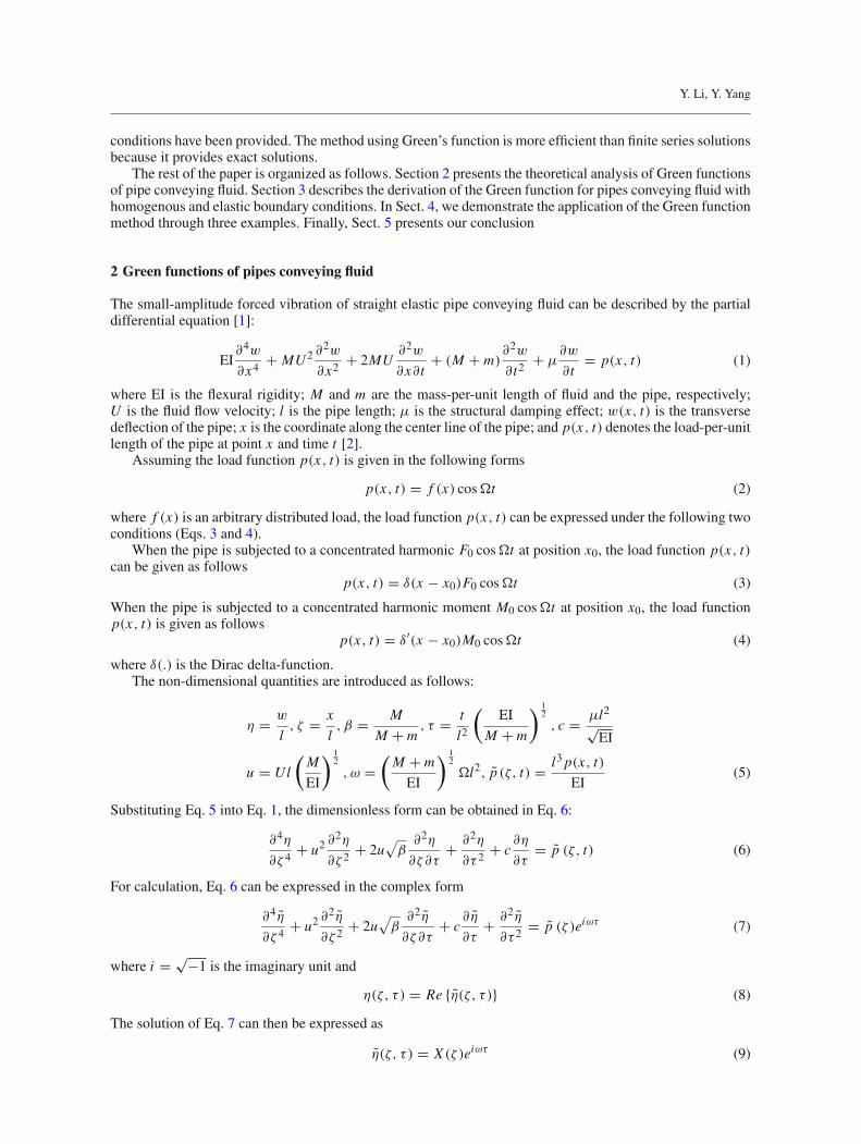
Fig. 4 Maximum deflection of different positions on the pipe
Fig. 5 Clamped–clamped conveying fluid pipe acted upon by a force f0 cos �t at intermediate position
Fig. 6 Elastic-support pipe conveying fluid
the position ζ = 0.8, the maximum deflection is η̃max = 0.014854; and at the position ζ = 1, the maximumdeflection is η̃max = 0.013785.
Figure 3 shows the effect of the flow velocity on the dynamic deflection of the system. Figures 2 and 3present the system deflection will not be in phase with the different position on the pipe and different flowvelocities, which should present right case about the gyroscopic term in Eq. (7). Figure 4 shows the maximumdeflection of different position on the pipe at the position (a = 0.6) of support B, which conforms to the realphysical case (Fig. 4).
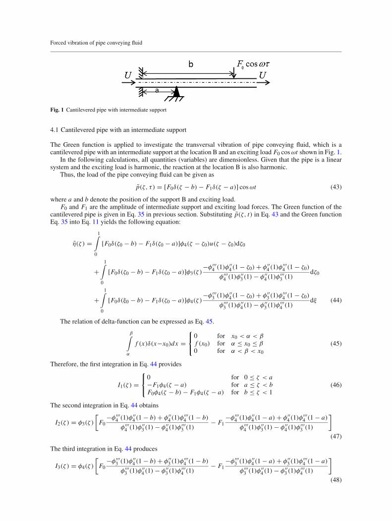
4.2 Comparing the solution of Green function with that of Galerkin
To show the correctness of the Green function method, the solution obtained from Green function was comparedwith that of Galerkin. A clamped–clamped pipe conveying fluid acted upon a force f0 cos ωt at the intermediateposition as depicted in Fig. 5
The dynamic deflection of the clamped–clamped pipe by Green function is expressed as follows:
η̃(ζ ) =1∫
0
f0δ(ζ0 − a)G(ζ, ζ0)dζ0 (53)

Y. Li, Y. Yang
Table 1 Dimensionless amplitude of dynamic deflection at ζ = 0.8536
Flow velocity Green’s function solution (exact) Galerkin’s solution (N = 2)numerical approximation
u = 0 0.002744 0.002943u = 4 0.005778 0.006213u = 5 0.017043 0.016924u = 6 0.011018 0.015108
Table 2 The number of terms N = 10, deflection with u = 5 at ζ = 0.8536
Green function solution Galerkin’s solution (N = 10)
Dynamical deflection 0.017043 0.017041
The expression of the Green function G(ζ, ξ) is Eq. 33 and a as the position of exciting load.
η̃(ζ ) = f0
⎧⎪⎪⎪⎪⎪⎪⎪⎪⎪⎨⎪⎪⎪⎪⎪⎪⎪⎪⎪⎩
φ3(ζ )−φ′
4(1)φ4(1−a)+φ4(1)φ′4(1−a)
φ′4(1)φ3(1)−φ4(1)φ′
3(1)
+ φ4(ζ )−φ′
3(1)φ4(1−a)+φ3(1)φ′4(1−a)
φ′3(1)φ4(1)−φ3(1)φ′
4(1); 0 ≤ ζ < a
φ4(ζ − a) + φ3(ζ )−φ′
4(1)φ4(1−a)+φ4(1)φ′4(1−a)
φ′4(1)φ3(1)−φ4(1)φ′
3(1)
+ φ4(ζ )−φ′
3(1)φ4(1−a)+φ3(1)φ′4(1−a)
φ′3(1)φ4(1)−φ3(1)φ′
4(1). a ≤ ζ ≤ 1
(54)
Using Eqs. (7) and (8), the dynamic response of the fluid-conveying pipe can be reduced to the following
η(ξ, τ ) = Re η̃(ξ) cos ωτ − I m η̃(ξ) sin ωτ (55)
The following non-dimensional parameters are used.
f0 = 2, β = 0.5, ω = 10.0, a = 0.5, c = 0.1. (56)
To verify the approach of the Green functions, the Green function solution and that of Galerkin [5] wascompared. Suppose η(ζ, τ ) can be approximated by
η(ξ, τ ) =N∑
r=1
ϕr (ζ )qr (τ ) (57)
where ϕr (ζ ) are eigenfunctions for free undamped vibration of clamped–clamped beam, and qr (τ ) the r-thgeneralized coordinate. N denotes the number of terms used in the Galerkin expansion. Substituting Eq. (57)into Eq. (7) and employing the orthogonal property of the modes, the partial differential equation of fluid-conveying pipe was reduced to an ordinary differential equation. The ordinary differential equations weresolved by Newmark and Newton-Raphson iteration method. Detailed application of the Galerkin method hasbeen described in previous report [5]. Table 1 shows that the results of both methods are close. The Greenfunction method has advantage of providing the exact solution. Table 2 shows that the Galerkin method solutionwith increasing N is more similar to the Green function solution.
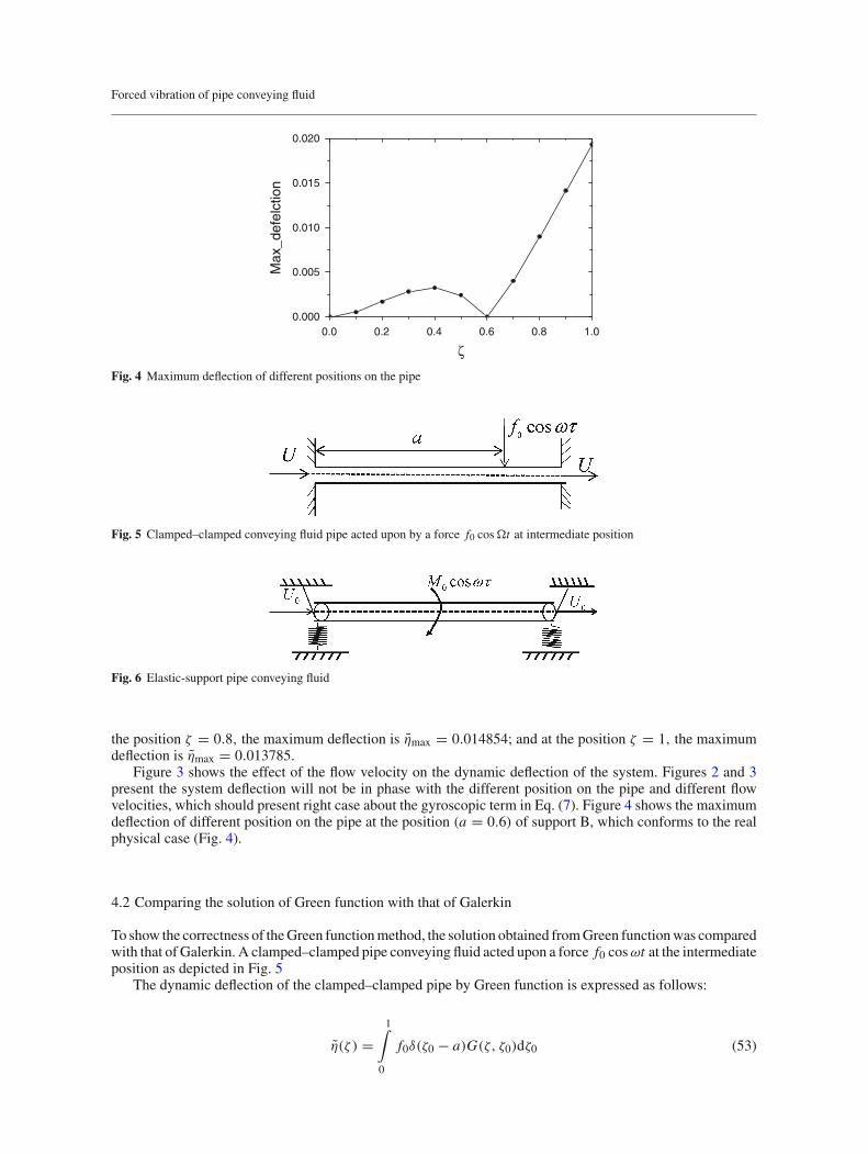
4.3 Pipe with elastic support
The fluid-conveying pipes with an elastic support at both ends as shown in Fig. 6 were also investigated.The harmonic momentum M0 cos ωt acts on the pipe at the position ζ = a. The dimensionless torsional andtranslational spring constants at the left-hand (right-hand) end of the pipe are denoted.
The dimensionless acted load is given by
p̃(ζ, t) = δ′(ζ − a)M0 cos ωτ (58)

Forced vibration of pipe conveying fluid
Fig. 7 Dimensionless dynamic deflection for the fluid-conveying pipe at ζ = 0.8, with the three dimensionless stiffness: (black)k = 4, (red) k = 40, and (blue) k = 100. (Color figure online)
Fig. 8 Dimensionless dynamic deflection for the conveying fluid pipe at ζ = 0.8, with the four dimensionless inner fluid velocities:(blue) u = 1, (red) u = 2.5, and (black) u = 3.5. (Color figure online)
The Green function of this pipe can be expressed by Eq. 42. The dynamic response of the elastic-supportfluid-conveying pipe can be written in the following form
w̃(ζ ) = M0
1∫0
δ′(ζ0 − a)G(ζ , ζ0)dζ0 (59)
Given the relation, the following can be obtained
1∫0
δ(n)(ξ − a)g(ξ)dξ = (−1)ng(n)(a), 0 ≤ a ≤ 1 (60)
The dynamic deflection can be represented as
w̃(ζ ) = −M0{−φ′4(ζ − a)u(ζ − a) + [−b11φ
′4(1 − a) − b12φ
′′4 (1 − a)
− b13φ′′′4 (1 − a) − b14φ
′′′′4 (1 − a)]φ1(ζ ) + φ2(ζ )[−b21φ
′4(1 − a) − b22φ
′′4 (1 − a)
− b23φ′′′4 (1 − a) − b24φ
′′′′4 (1 − a)] + kT 1φ3(ζ )[−b21φ
′4(1 − a) − b22φ
′′4 (1 − a)
− b23φ′′′4 (1 − a) − b24φ
′′′′4 (1 − a)] − k1φ4(ζ )[−b11φ
′4(1 − a) − b12φ
′′4 (1 − a)
− b13φ′′′4 (1 − a) − b14φ
′′′′4 (1 − a)]} (61)

Y. Li, Y. Yang
0.0
0.5
1.0
1.5
2.0
2.5D
efel
ctio
n
Def
elct
ion
Def
elct
ion
Def
elct
ion
External excited frequency ω External excited frequency ω
External excited frequency ωExternal excited frequency ω
(a)
0.0
0.5
1.0
1.5
2.0 (b)
0.00
0.01
0.02
0.03
0.04
0.05
0.06
0.07
0.08
(c)
1.0 1.5 2.0 2.5 3.0 4.6 4.8 5.0 5.2 5.4 5.6 5.8 6.0
26.7 27.0 27.3 27.6 27.9 28.2 28.5 67.5 67.8 68.1 68.4 68.7 69.0 69.30.00
0.02
0.04
0.06
0.08
0.10
0.12
0.14 (d)
Fig. 9 Dimensionless dynamical deflection for the conveying fluid pipe at ζ = 0.8 with the different dimensionless externalexcited frequencies: a near ω1, b near ω2, c near ω3, and d near ω4
Using Eqs. (7) and (8), the dynamic response of the fluid-conveying pipe can be reduced to
η(ξ, τ ) = Re w̃(ξ) cos ωτ − I m w̃(ξ) sin ωτ (62)
The non-dimensional parameters were selected as follows
β = 0.5, a = 0.5, c = 0.1, k1 = k2 = kt1 = kt2 = k (63)
The impact of the parameters on the dynamic deflection of pipe conveying fluid was investigated in thissection. The results and analysis are presented in Figs. 7, 8, and 9. Figure 7 shows the dimensionless dynamicdeflection for the fluid-conveying pipes at ζ = 0.8, with the parameters ω = 10, M0 = 0.1, u = 3, thedifferent stiffness: (blue) k = 4, (red) k = 40, and (black) k = 100. Figure 8 shows the system response willnot be in phase, which should be the right case, because of the gyroscopic term in Eq. (7). Varying the valueof the stiffness leads to the change in natural frequencies and increase or decrease in the amplitude of thedynamic deflection of the system. This phenomenon is dependent on, whether or not the natural frequenciesof the system approach the excited frequency ω. Figure 8 shows the dimensionless dynamic deflection underdifferent inner flow velocities with parameters k = 4, ω = 10, M0 = 0.1. The inner flow velocity of the pipehas affects the deflection. Varying the value of flow velocity leads to change in natural frequencies. Whenthe parameters are u = 3, M0 = 0.1, k = 4, and the other parameters remain unchanged, Fig. 9 shows thedimensionless dynamic deflection under different excited frequencies. When the external excited frequencyω approaches to the first fourth natural frequency ωi , i = 1, 2, 3, 4, the amplitude should be large. Based onFig. 9, the first fourth natural frequencies can be obtained
ω1 ≈ 1.9, ω2 ≈ 5.3, ω3 ≈ 27.6, ω4 ≈ 68.8 (64)
These results that are similar with the first four natural frequencies of the pipe conveying fluid are computed bythe DQM method as follows: ω1 = 1.9, ω2 = 5.3, ω3 = 27.5, ω4 = 68.9. Based on the principal, the Greenfunction method can be applied to obtain natural frequency of the pipe conveying fluid.

Forced vibration of pipe conveying fluid
5 Conclusion
The paper presented the Green function method to study the dynamic response of pipe conveying fluid underforced vibration. This method yielded exact solutions in a closed form. Three examples of the pipe conveyingfluid were analyzed, and the results showed the validity of the Green function method. The natural frequencyof the pipe conveying fluid can be obtained by the Green function method.
Acknowledgments The research was partially supported by the National Natural Science Foundation of China (11102170),Sichuan province science and technology innovation team (2013TD0004) and Fund Project of Department of Education ofSichuan Province (No. 11ZB255). The authors thank the anonymous reviewers for their helpful suggestions.
References
1. Bourrieres. F.J.: Sur un phenomene d’oscillations auto-entretenue en mecanique des fluides reels. Publications Scientifiqueset Techniques du Ministere de l’Air 147 (1939)
2. Paidoussis, M.: Fluid–Structure Interactions: Slender Structures and Axial Flow, Vol. 1. London: Academic Press (1998)3. Jin, J., Song, Z.: Parametric resonances of supported pipes conveying pulsating fluid. J. Fluids Struct. 20, 763–783 (2005)4. Doaré, O., Langre, E.de : The flow-induced instability of long hanging pipes. Eur. J. Mech. A/Solids 21, 857–867 (2002)5. Chen, S.S.: Forced vibration of a cantilevered tube conveying fluid. J. Acoust. Soc. Am. 48, 773–775 (2005)6. Olson, L., Jamison, D.: Application of a general purpose finite element method to elastic pipes conveying fluid. J. Fluids
Struct. 11, 207–222 (1997)7. Qian, Q., Wang, L., Ni, Q.: Instability of simply supported pipes conveying fluid under thermal loads. Mech. Res. Com-
mun. 36, 413–417 (2009)8. Ni, Q., Zhang, Z., Wang, L.: Application of the differential transformation method to vibration analysis of pipes conveying
fluid. Appl. Math. Comput. 217, 7028–7038 (2011)9. Nicholson, J.W., Bergman, L.A.: Free vibration of combined dynamical systems. J. Eng. Mech. 112, 1–13 (1986)
10. Kukla, S., Posiadala, B.: Free vibrations of beams with elastically mounted masses. J. Sound Vib. 175, 557–564 (1994)11. Abu-Hilal, M.: Forced vibration of Euler–Bernoulli beams by means of dynamic Green functions. J. Sound Vib. 267,
191–207 (2003)12. Li, X., Zhao, X., Li, Y.: Green’s functions of the forced vibration of Timoshenko beams with damping effect. J. Sound
Vib. 333, 1781–1795 (2014)13. Caddemi, S., Caliò, I., Cannizzaro, F.: Closed-form solutions for stepped Timoshenko beams with internal singularities and
along-axis external supports. Arch. Appl. Mech. 83, 559–577 (2013)14. Failla, G.: Closed-form solutions for Euler–Bernoulli arbitrary discontinuous beams. Arch. Appl. Mech. 81, 605–628 (2011)15. Failla, G., Santini, A.: On Euler–Bernoulli discontinuous beam solutions via uniform-beam Green’s functions. Int. J. Solids
Struct. 44, 7666–7687 (2007)