FORCE CONTROL OF A HYDRAULIC SERVO SYSTEM _____________________________________________________

A Thesis presented to the Faculty of the Graduate School

University of Missouri

________________________________

In partial Fulfillment Of the Requirements for the Degree

Master of Science

________________________________

by JOSEPH L. KENNEDY

Dr. Roger Fales, Thesis Supervisor

MAY 2009

The undersigned, appointed by the Dean of the Graduate School, have examined the thesis entitled

FORCE CONTROL OF A HYDRAULIC SERVO SYSTEM

Presented by Joseph L. Kennedy A candidate for the degree of Master of Science And hereby certify that in their opinion it is worthy of acceptance.

__________________________________ Dr. Roger Fales

__________________________________ Dr. Noah Mannring

__________________________________ Dr. William Jacoby

…To my father, Jerry Lee Kennedy

ii

ACKNOWLEDGEMENTS

I would like to thank Dr. Roger Fales for his contribution to my research. Dr.

Fales introduced me to control systems as an undergraduate at MU and assisted me

throughout my Master’s program. My Master’s thesis would not have been possible

without his influence and participation. I would also like to thank Dr. Noah Manring for

introducing me to hydraulic systems as a undergraduate. Finally, I would like to thanks

all of the teachers and faculty in the Mechanical and Aerospace department at MU for

making my Master’s program so enjoyable.

iii

TABLE OF CONTENTS

ACKNOWLEDGEMENTS................................................................................................ ii LIST OF ILLUSTRATIONS...............................................................................................v LIST OF TABLES............................................................................................................ vii LIST OF ABBREVIATIONS.......................................................................................... viii LIST OF SYMBOLS..........................................................................................................ix ABSTRACT ..................................................................................................................... xii Chapter 1. INTRODUCTION ......................................................................................................1

1.1 Force Feedback Control Systems ......................................................................1 1.2 Background Information and Previous Work....................................................2 1.3 Goals/Overview .................................................................................................4

2. EXPERIMENTAL SETUP ........................................................................................6 2.1 Mechanical Setup...............................................................................................6 2.2 Data Acquisition Setup ......................................................................................8

2.3 Input/Output Characteristics of the System.......................................................9 3. MODELING THE SYSTEM ...................................................................................12 3.1 Open-Loop Linear Modeling...........................................................................12 3.2 Transfer Function Models................................................................................14 3.3 DC-gain of the Servo System ..........................................................................17 4. CONTROLLER DESIGN ........................................................................................22 4.1 Bandwidth Limitation......................................................................................22

iv

4.2 Controller Overview/Selection ........................................................................23 5. CLOSED-LOOP PERFORMANCE ........................................................................28

5.1 Time Domain Performance..............................................................................28 5.2 Frequency Domain Performance .....................................................................32

6. NOMINAL/ROBUST STABILITY AND PERFORMANCE.................................39 6.1 Dynamic and Parametric Uncertainties ...........................................................39

6.2 Performance Weight ........................................................................................41

6.3 Obtaining P and N Matrixes ............................................................................43

6.4 Defining Stability/Performance and the Structured Singular Value................46 6.5 Nominal and Robust Stability..........................................................................47

6.6 Nominal and Robust Performance...................................................................49

7. CONCLUSION.........................................................................................................53

7.1 Experimental Results .......................................................................................53 7.2 Future Work.....................................................................................................55

BIBLIOGRAPHY..............................................................................................................57

v

LIST OF ILLUSTRATIONS Figure Page 1. Hydraulic servo system..................................................................................................7 2. Schematic of the servo system.......................................................................................7 3. Hydraulic power unit. ....................................................................................................7  4. Block diagram of the hydraulic servo system (dotted and bold arrows represent

electric and hydraulic connections, respectively). .........................................................8  5. Electrical equipment. .....................................................................................................9  6. Bode magnitude of the experimental and analytical results. .......................................15  7. Bode phase of the experimental and analytical results. ...............................................16  8. Output force (left) and DC-gain (right) as a function of input voltage. ......................19  9. Block diagram of the closed-loop control system. ......................................................23  10. CL unit step response with no control (i.e. K =1 in Fig. 9). ........................................23  11. OL frequency response of the shaped plants and shaped plants with H∞ control. ......27  12. CL response of the P control systems with a reference step input from -1000 to

1000 lbf (top) and 1000 to -1000 lbf (bottom). ...........................................................29  13. CL response of the PID control system with a reference step input from -1000 to

1000 lbf (top) and 1000 to -1000 lbf (bottom). ...........................................................29  14. CL response of the H∞ control systems with a reference step input from -1000 to

1000 lbf (top) and 1000 to -1000 lbf (bottom). ...........................................................30  15. CL response of the system with a reference step input from -1000 to 1000 lbf

(top) and 1000 to -1000 lbf (bottom)...........................................................................30  16. Open-loop response to a chirp signal with magnitude of 0.5 V, offset of 0 V, and

frequency range from 0 to 50 Hz.................................................................................34  17. Bode magnitude plot of the normalized OL and CL P control (top), PID control

(middle), and H∞ control (bottom) cases......................................................................34 

vi

18. Bode phase plot of the normalized OL and CL P control (top), PID control

(middle), and H∞ control (bottom) cases......................................................................35  19. Input voltage to the servo-valve amplifier for CL control with KH# (top) and KH#

(bottom). ......................................................................................................................38  20. Dynamic MU for trials (a-c) and resulting uncertainty TF..........................................40  21. CL system with multiplicative uncertainties and performance measured at the

error..............................................................................................................................43  22. Inverse of the performance weight (i.e. 1/| wP(jω)|) ....................................................43  23. P and N matrixes..........................................................................................................44  24. Robust stability (i.e.

�

µΔ (N11 (ω )) < 1) for rk = 0.095 (top), rk = 0.379 (middle) and rk = 1 (bottom). ................................................................................................................49 

25. Nominal performance (i.e. µ (N22)) with A = 0.1, M = 3, and ωBR = 10 Hz. ...............51 

vii

LIST OF TABLES

Table Page 1. Average DC-gain values (all values in lbf/V). ............................................................20 2. Crossover frequencies and corresponding phase lags for the shaped plants and

shaped plants with H∞ control. ....................................................................................27 3. Time domain performance for system and models......................................................32 4. Bandwidth frequencies for the OL and CL frequency response and corresponding

saturation frequencies. .................................................................................................37 5. Stability and performance of each control system.......................................................48 

viii

LIST OF ABBREVIATIONS Abbreviation Meaning CL ..............................Closed-loop DAC...........................Data Acquisition FFT ............................Fast Fourier Transformation LHP............................Left Half Plane MU.............................Multiplicative Uncertainty NP ..............................Nominal Performance NS ..............................Nominal Stability OL..............................Open-loop P .................................Proportional PID.............................Proportional-Integral-Derivative QFT............................Quantitative Feedback Theory RHP............................Right Half Plane RP ..............................Robust Performance RS ..............................Robust Stability SS...............................Steady state SSV............................Structured Singular Value TF...............................Transfer Function

ix

LIST OF SYMBOLS Symbol Definition A.................................Low frequency performance requirment A, B, C, D ...................State-space representation of the shaped plant Ao................................Cross-sectional area within the needle valve Cd ...............................Volumetric flow rate through needle valve DC..............................DC-gain of the servo system dPs ..............................Polynomial for the static DC-gain vs. Input Voltage relationship dPt ..............................Polynomial for the triangular DC-gain vs. Input Voltage relationship e..................................Error signal from closed-loop system

�

˙ e .................................First derivative of the error

�

˙ ̇ e .................................Second derivative of the error Fa................................Actual force output from closed-loop system Fd................................Desired force output from closed-loop system G ................................Plant G3 ...............................3rd-order transfer function of the closed-loop servo responce G4 ...............................4th-order transfer function of the closed-loop servo responce Gn ...............................Nominal plant model Gp,d .............................Dynamically perturbed plant model Gp,p .............................Parametrically perturbed plant model kmax .............................Maximum gain value kmin..............................Minimum gain value

x

K.................................Controller KD...............................Derivative gain KH...............................H∞ controller KH3 .............................H∞ controller found from the shaped plant KPIDG3 KH4 .............................H∞ controller found from the shaped plant KPIDG4 KI................................Integral gain KP ...............................P Controller (proportional gain) KPID ............................PID Controller KPIDG3 ........................Shaped plant with 3rd-order model KPIDG4 ........................Shaped plant with 4th-order model L .................................Any complex matrix lI ................................Maximum multiplicative uncertainty M................................High frequency performance requirment n ................................order of the transfer function model N.................................N-matrix N11, N12, N21, N22 ........Elements of the N-matrix P .................................Generalized plant model (P-matrix) P11, P12, P21, P22 .........Elements of the P-matrix PA ...............................Actuator pressure on the side A PB ...............................Actuator pressure on the side B Ps ................................Polynomial for the static input-output relationship Psu ..............................Supply pressure from hydraulic power unit

xi

Pt ................................Polynomial for the triangular Input Voltage vs. Output Force relationship Δp ...............................Pressure difference across the needle valve Q ................................Volumetric flow rate through needle valve rk ................................Relative magnitude of the gain uncertainty wI................................Dynamic uncertainty transfer function wP ...............................Performance weight transfer function Z, X.............................Unique definite solutions to Riccati equations Δ .................................Any real scalar ΔI ................................Any stable transfer function such that

�

ΔI ≤ 1 ΔP ...............................Fictitious uncertainty block ζ .................................Damping ratio θ .................................Time delay in seconds µ .................................Structured singular value ρ .................................Hydraulic fluid density ρs ................................Spectral radius (maximum singular value)

�

σ ................................Maximum singular value ω.................................Frequency ranging from 0 to 100 Hz ωB ...............................Closed-loop bandwidth frequency

�

ωB* ..............................Acheivable bandwidth for a linear system with a right-half-plane

zero ωBR .............................Approximate bandwidth requirement ωn ...............................Natural frequency

xii

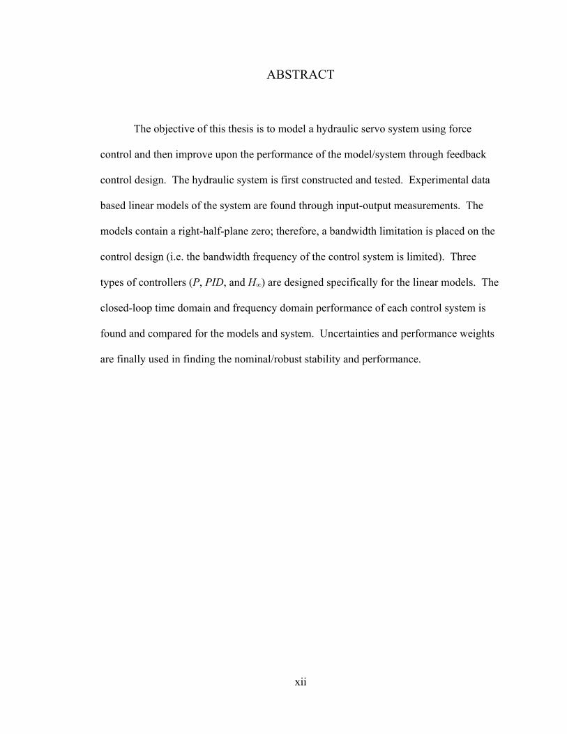
ABSTRACT

The objective of this thesis is to model a hydraulic servo system using force

control and then improve upon the performance of the model/system through feedback

control design. The hydraulic system is first constructed and tested. Experimental data

based linear models of the system are found through input-output measurements. The

models contain a right-half-plane zero; therefore, a bandwidth limitation is placed on the

control design (i.e. the bandwidth frequency of the control system is limited). Three

types of controllers (P, PID, and H∞) are designed specifically for the linear models. The

closed-loop time domain and frequency domain performance of each control system is

found and compared for the models and system. Uncertainties and performance weights

are finally used in finding the nominal/robust stability and performance.

1

Chapter 1.

INTRODUCTION

1.1 Force Feedback Control Systems

Hydraulic control valves (such as a servo-valve) are used within hydraulic control

systems to accurately regulate the output of the entire system. The valve provides the

interface between the hydraulic power unit and the output device, in this case a linear

actuator. The control valve has the ability to receive a signal from a control system in

order for the output of the system to track a desired input [1]. Using force feedback to

control a hydraulic system allows the user to control the force output from a linear

actuator by supplying the control system with a desired force reference signal.

Controllers are designed specifically for the closed-loop (CL) system to improve

performance (i.e. improve the ability of the system to track a given input signal) and

stability (i.e. the ability of the system to adjust to uncertainties).

There are many types of controllers that can be implemented into a CL control

system, each of which adds different performance characteristics. The process used in

this paper for obtaining CL control is as follows. A linear model (linear transfer

function) representing the open-loop (OL) frequency domain performance of the servo

system is found through analyzing input-output measurements at given operating points

over a range of frequencies. A controller is designed specifically for the linear model and

then tested on the servo system to find the CL time domain and frequency domain

performance of the system. This process is repeated for different linear models and

controllers.

2

Once a control system is designed and tested, the nominal/robust stability and

performance of that control system can be found. The nominal stability and performance

are found in relation to the nominal plant (i.e. the linear model found from the input-

output measurements). The uncertainties within the OL system (both dynamic and

parametric) are used in finding a perturbed plant (i.e. the nominal plant plus all

perturbations). The perturbed plant is used in evaluating the robust stability and

performance of the CL system (a performance weight transfer function is also required in

finding robust performance).

1.2 Background Information and Previous Work

Hydraulic actuators have several non-lineararities due mainly to servo-valve flow

and pressure characteristics [2]. The method used in this thesis is based on the

linearization of the non-linear dynamics of a hydraulic system about given operating

points. The stability and performance of a linear control system is, therefore, only

achievable at or near the operating points which the controller is designed around. Linear

models are commonly used given their relative simplicity and accuracy at a given

operating point (point of interest). In order to model a full range of operating points, a

different method must be considered. One such method considers non-linear Quantitative

Feedback Theory (QFT) where the non-linear plant is replaced with a “family of linear

time invariant transfer functions” [2]. The linear transfer functions are based on

experimental input-output measurements (the plant models in the this thesis are found

through a similar input-output measurement approach). Non-linear QFT robust control

methodology can then be used to design a force controller that is of “low-order” and that

3

can “maintain satisfactory performance against uncertainties” [2]. A second method for

modeling an entire system (not just specific operating points) uses Input-Output

Feedback Linearization, which requires full state feedback (an observer can be used to

estimate states that can not be measured) [3]. In this approach, no particular operating

point is used in obtaining a linear model of the system. Therefore, the performance of a

given control system is not influenced by its proximity to the set of operating points,

which results in better performance over the entire operating range of the system [3].

Either of the control design methods discussed here can be implemented if the linear

method does not result in satisfactory performance due to the uncertainties of the system

and/or if a wide range of operating points are needed.

Force control on various hydraulic servo systems has been documented. The

system given by [4] is used to simulate modern fly-by-wire flight control systems for

testing primary fight actuators. In this application, a “high-bandwidth force response” is

needed to simulate the aerodynamic loads that are applied to the control surfaces during

flight [4]. Uncertainties in structural stiffness and hydraulic plant parameters require a

“robust approach to the design of the force control” [4]. Higher bandwidth frequencies

correlate to faster response/rise times and improved robustness is associated with

increased stability. Therefore, the control system must have a balance between stability

and speed of response. By knowing the performance requirements of the desired system,

a specific controller can be chosen based on its performance characteristics.

The modeling and control design process outlined by [4] is similar to the process

used in this thesis; however, the experimental setup is different. The movement of the

main loading actuator is restricted in this thesis. In contrast, [4] allows movement by

4

connecting the main loading actuator to a secondary actuator via a lever arm. The

experimental setup given by [2] also allows actuator movement by connecting the

actuator rod to a spring. Obtaining a control system for the case with actuator movement

requires slight adjustments to the control design process outlined in this thesis (i.e. a

correction to the force demand must be made based on the displacement and/or velocity

of the loading actuator). The experimental setup in this thesis also incorporates a needle

valve to regulate hydraulic fluid flow between the high and low-pressure side of the

actuator. The experimental setups given by [2] and [4] do not have such a capability.

Finally, this thesis gives extensive uncertainty analysis on the control systems, while [2]

and [4] only focus on control design.

1.3 Goals/Overview

The goals of this thesis are as follows: construct the hydraulic servo system for

lab testing, perform lab tests to create a dynamic model of the servo system, quantify

performance limitations to find the highest possible theoretical performance (limitations

include saturation and pole/zero locations of the model), increase the performance of the

system through control design, analyze the time and frequency domain performance of

the control systems, and test for nominal/robust stability and performance. Chapter 2

outlines the experimental setup for the mechanical system and data acquisition process

along with a description of the input-output characteristics of the system. The dynamic

modeling process is given in Chapter 3, and the performance limitations and control

design are discussed in Chapter 4. The time and frequency domain performance of each

control system are found in Chapter 5, and the nominal/robust stability and performance

5

are determined in Chapter 6. Chapter 7 is an overview of the findings and also contains

suggestions for future work.

6

Chapter 2.

EXPERIMENTAL SETUP

2.1 Mechanical Setup

A picture and schematic of the hydraulic servo system are shown in Fig. 1 and

Fig. 2, respectively. A double-rod actuator (front and rear piston areas are equal) is used

as the force output devise. The rear, B, actuator rod is enclosed within a protective

casing. The front, A, actuator rod is connected to a load cell, which in turn is attached to

a stiff steel link. The link is bolted to a bracket that is secured to the same I-beam as the

actuator, impeding any movement of the actuator rod during loading. Two pressure

sensors are placed on either side of the piston to record fluid pressures within the actuator

(i.e. PA and PB in Fig. 2). A third pressure sensor records the supply pressure, Psu, from

the hydraulic power unit. The power unit (shown in Fig. 3) uses an electric motor and

hydraulic pump to supply the system with a constant Psu. A hydraulic line connects side

A and B of the actuator allowing hydraulic fluid to leak from the high to low-pressure

side. A needle valve is placed on the leakage line to control the amount of fluid that can

be passed from one side of the actuator to the other.

7

Fig. 1. Hydraulic servo system.

Fig. 2. Schematic of the servo system.

Fig. 3. Hydraulic power unit.

8

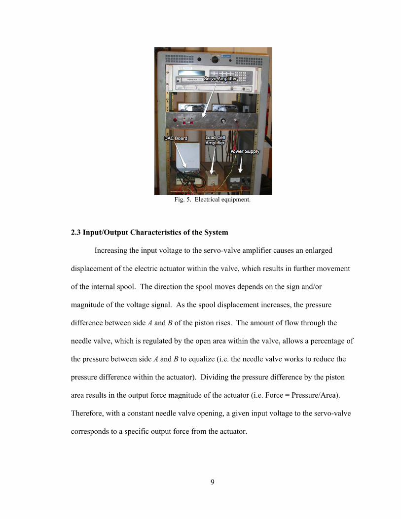
2.2 Data Acquisition Setup

A block diagram of the hydraulic servo system is shown in Fig. 4, and a photo of

the electrical equipment is given in Fig. 5. The hydraulic pump supplies the servo-

valve/actuator with a constant Psu. The PC sends an input voltage signal through an

analog output port on the data acquisition (DAC) board where it is converted from a

digital-to-analog signal, to the servo amplifier. The input signal is then sent from the

amplifier to the servo-valve. A power supply provides the load cell and pressure sensors

with a required 20 V. The output voltage from each sensor is sent to the PC through

analog input ports on the DAC board where it is converted from an analog-to-digital

signal (the output signal from the load cell is passed through an amplifier before it is sent

to the DAC board). The load cell signal, along with some type of control system, can

then be used to create closed-loop (CL) force control for the system. Simulink® and

Matlab® are used as the user interface to generate and analyze all data to and from the

PC.

Fig. 4. Block diagram of the hydraulic servo system (dotted and bold arrows represent

electric and hydraulic connections, respectively).

9

Fig. 5. Electrical equipment.

2.3 Input/Output Characteristics of the System

Increasing the input voltage to the servo-valve amplifier causes an enlarged

displacement of the electric actuator within the valve, which results in further movement

of the internal spool. The direction the spool moves depends on the sign and/or

magnitude of the voltage signal. As the spool displacement increases, the pressure

difference between side A and B of the piston rises. The amount of flow through the

needle valve, which is regulated by the open area within the valve, allows a percentage of

the pressure between side A and B to equalize (i.e. the needle valve works to reduce the

pressure difference within the actuator). Dividing the pressure difference by the piston

area results in the output force magnitude of the actuator (i.e. Force = Pressure/Area).

Therefore, with a constant needle valve opening, a given input voltage to the servo-valve

corresponds to a specific output force from the actuator.

10

The open area (cross-sectional area) inside the needle valve has a direct

correlation to the volumetric flow rate, Q, through the valve. The needle valve behaves

as an orifice. The flow rate through an orifice is given as

�

Q = AoCd2ρΔp , (1)

where Ao is the cross-sectional area within the needle valve, Cd is the discharge

coefficient (constant), ρ is the fluid density (assumed to remain constant), and Δp is the

pressure difference across the orifice (i.e. the pressure difference between side A and B of

the actuator). Increasing Ao or Δp will increase the flow rate through the valve. As fluid

flows from the high to low pressure side of the actuator, the pressure difference is

reduced, which reduces the magnitude of the output force. Therefore, the relationship

between input voltage and output force is dependent on Ao. As Ao increases, a larger

pressure can be equalized within the actuator, which results in a smaller force. Therefore,

in order for the output force to remain constant, the input voltage to the servo-valve

amplifier must be increased as Ao is increased.

The hydraulic power unit, shown in Fig. 3, supplies the servo system with a

constant Psu of 1000 psi. The double-rod actuator has a piston area of 5.23 in2 on both

side A and B. Therefore, the maximum/minimum output force from the actuator is

approximately ±5200 lbf. With no leakage (i.e. the needle valve is completely closed),

the system achieves the maximum/minimum output force at an input voltage to the

amplifier of ±0.25 V, which is small given the servo amplifier has an operational range of

±5 V (as specified by the manufacturer). As stated above, increasing Q changes the

relationship between input voltage and output force. Therefore, to increase the voltage

11

range for experimentation, the needle valve is opened to increase the volumetric flow

through the needle valve. The valve is adjusted until an input of ±2 V results in a

maximum/minimum output force of ±4800 lbf. When leakage across the actuator is

allowed, the pressure difference between side A and B of the piston is reduced. Thus, the

maximum/minimum output force with leakage (±4800 lbf) is less than the

maximum/minimum output force without leakage (±5200 lbf).

12

Chapter 3.

MODELING THE SYSTEM

3.1 Open-Loop Linear Modeling

An OL linear model of the hydraulic system at a given operating point can be

found through experimental input-output measurements. The experimental process for

attaining a linear model is as follows.

1. Choose an appropriate input voltage signal.

2. Run experiment and record input voltage data to the servo-valve amplifier and

output force data from the load cell.

3. Analyze the input-output data using a fast Fourier transformation (FFT) to find a

Bode magnitude and phase plot of the system.

4. Once data is collected over a range of frequencies, a transfer function (TF) best

representing the OL response of the system can be found.

The simplest way in finding a linear OL model is to choose an input signal that contains a

desired range of frequencies. Since an entire frequency range is represented in the input

signal, only one experimental test is needed to find a complete OL model of the system.

One signal with such a characteristic is called a chirp signal. A chirp signal is a sine

wave whose frequency increases with time and whose amplitude remains constant. The

user defines the frequency range and run-time of the signal.

A chirp signal with amplitude of 0.5 V and a frequency range from 0 to 150 Hz is

sent to the servo-valve amplifier for a period of 200 seconds. Varying the offset of the

chirp signal allows the valve to be tested at different operating points. The purpose of

13

testing at separate operating points is to find a linear model that best represents the

system over a range of inputs. Three separate chirp signals with offsets at 0.25, 0, and -

0.25 V are used for testing the servo system. Once the experiments are complete, the

input and output data are analyzed using a FFT to obtain the Bode magnitude and phase

plots shown in Fig. 6 and Fig. 7, respectively (refer to “Chirp Data”). The Matlab®

command fft is used in calculating the FFT of the experimental voltage and force data.

The results for the chirp signals with input offsets at 0.25, 0, and -0.25 V are represented

by trial (a), (b), and (c), respectively. The response of the system is negligible at

frequencies > 100 Hz; therefore, only data ≤ 100 Hz is considered. As the frequency

increases, the range of the experimental data increases (i.e. there is a larger variance or

uncertainty associated with data at higher frequencies). Averaging data values at a given

frequency with values near that frequency can filter out the variation in the magnitude

and phase data, which results in a set of closely packed data points representing the mean

of the experimental results (see “Filtered Chirp Data” in Fig. 6 and Fig. 7).

The OL frequency domain performance of the servo system can also be found

using standard sine waves. A sine wave with a frequency ≤ 100 Hz and magnitude of 0.5

V is first sent to the servo-valve amplifier. The magnitude and phase lag of the system

can then be found by directly comparing the input and output signals. The main

drawback of performing such a test is that several experiments are required to obtain the

OL response over the desired frequency range. In contrast, the sine test is useful in

verifying the data acquisition process used with the chirp signal. A sine test is performed

at 8 separate frequencies for each offset defined by trials (a-c). The magnitude and phase

results for the sine test are shown as “*” in Fig. 6 and Fig. 7, respectively. The sine test

14

data is very similar to the filtered chirp signal data in trials (a-c); therefore, the data

acquisition process used in obtaining the OL chirp response is considered accurate.

The experimental data can now be used in finding a linear TF that best matches

the system characteristics. Selected magnitude, phase, and frequency values from the

filtered chirp data are inputted into the Matlab® command fitsys to find a TF that best

represents the experimental OL frequency domain data (fitsys fits frequency response

data with a TF of order n using frequency dependent weights). It is desired to have a

single TF that approximates the frequency domain performance of the system at each

operating point (each chirp signal offset). Trial (b) corresponds to the input signal with

an offset of 0 V, which is bounded by trails (a) and (c) with offsets of 0.25 and -0.25 V,

respectively. Given the nonlinearities that exist in the servo system, models designed at

two separate operating points will tend to differ more from one another as the distance

between the operating points (offsets) increase. Therefore, a TF designed with data from

trail (b), appose to trial (b) or (c), is expected to more closely model the response of the

system at all three offsets.

3.2 Transfer Function Models

A 3rd-order, G3, and 4th-order, G4, model of the servo system found using data

from trial (b) are given as

�

G3 =1.705e4(s− 445)

(s2 + 365s +1.705e4)(s + 445)⎛ ⎝ ⎜

⎞ ⎠ ⎟ DC (2)

and

�

G4 =(3.283s2 +1352s + 2.624e6)(s− 2000)

(s3 + 363s2 + 6.894e4s + 2.624e6)(s + 2000)⎛ ⎝ ⎜

⎞ ⎠ ⎟ DC ,

(3)

15

where DC is the DC-gain of the system (the DC-gain is discussed in length in section

3.3). Both models closely match the experimental phase data for each trial over the full

range of frequencies (see Fig. 7). Conversely, only G4 matches the experimental

magnitude data over all frequencies (see Fig. 6). At approximately 20 Hz G3 begins to

diverge away from the experimental magnitude results, which suggests that the system

behaves as a higher order model (i.e. n > 3) at higher frequencies. Nevertheless, G3 is not

discarded given that it is a good representation of the system at lower frequencies.

Fig. 6. Bode magnitude of the experimental and analytical results.

100

101

102

20

30

40

50

60

70

(a) Frequency (Hz)

Ma

gn

itu

de

(d

B)

Chirp Data

Filtered Chirp Data

Sign Test Data

3rd Order Model (G3)

4th Order Model (G4)

100

101

102

20

30

40

50

60

70

(c) Frequency (Hz)

Ma

gn

itu

de

(d

B)

100

101

102

20

30

40

50

60

70

(b) Frequency (Hz)

Ma

gn

itu

de

(d

B)

DC!gain = 3900 lbf/V

DC!gain = 3700 lbf/V

DC!gain = 3200 lbf/V

Student Version of MATLAB

16

Fig. 7. Bode phase of the experimental and analytical results.

The linear models given in Eqs. (2) and (3) contain a right-half-plane (RHP) zero

associated with a 1st-order time delay approximation given as

�

e−θs ≈s− 2 /θs + 2 /θ

, (4)

where θ is the time delay in seconds [5]. The time delay for G3 and G4 is 4.5 and 1 ms,

respectively. The difference in time delay between G3 and G4 is due mainly to un-

modeled dynamics associated with the 3rd-order model, which influence the time delay

approximation (the un-modeled dynamics of G3 are shown in Fig. 6). Given that G4

better models the OL response of the system, a time delay of 1 ms is a better

100

101

102

!250

!200

!150

!100

!50

0

(a) Frequency (Hz)P

hase (

deg)

Chirp Data

Filtered Chirp Data

Sign Test Data

3rd Order Model (G3)

4th Order Model (G4)

100

101

102

!250

!200

!150

!100

!50

0

(c) Frequency (Hz)

Phase (

deg)

100

101

102

!250

!200

!150

!100

!50

0

(b) Frequency (Hz)

Phase (

deg)

Student Version of MATLAB

17

approximation of the real time delay of the servo system. A system with a time delay

(i.e. RHP zero) has CL control performance limitations (bandwidth limitations) discussed

in Chapter 4.1.

3.3 DC-gain of the Servo System

The DC-gain of the system (represented by DC in Eqs. (2) and (3)) corresponds to

the change in output force given a change in input voltage (i.e. the slope of output vs.

input curve). There are several ways in finding the relationship between the in the input

and output of the servo system. The most straightforward procedure is to give the system

a constant/static input voltage and record the corresponding output force. This procedure

must be repeated over a range of input voltages to acquire an input-output correlation.

Depending on the initial voltage of the system, the output force at a given input voltage is

found to vary. In other words, the output force at 0 V is different when the system is

stepped from -2 to 0 V than when stepped from 2 to 0 V. This inconsistency in the output

of a system is referred to as hysteresis. The main cause of hysteresis in the case of a

servo-valve is static friction or “stiction” between the moving parts of the valve [1]. One

way to reduce stiction is to keep the valve in constant movement by superimposing a

dither signal (i.e. a sine wave with given magnitude and frequency) onto the input signal.

The magnitude and frequency of the chirp signal must be chosen to keep the stiction

within the valve at a minimum without influencing the output force signal.

A second testing procedure for finding an input-output relationship is to give the

system a “slow” moving triangular wave over a given range of input voltages (the signal

is considered “slow” in that the slope of voltage/time is small). The purpose of using a

18

slow triangular wave is to define the static relationship between a given input voltage and

the resulting output force as the input is increased and decreased. Again, the system has

hysteresis resulting from the inconsistencies in the way the system responds as the input

voltage is increased (positive slope of the triangular wave) and decreased (negative slope

of the triangular wave). Therefore, a dither signal is also applied to the triangular input

wave. A dither signal of amplitude 0.4 V and frequency 175 Hz is found to best reduce

the valve hysteresis for both the static and triangular tests without affecting the output

signal.

The input voltage vs. output force plot for the static and triangular tests are shown

in Fig. 8. The static input-output test is performed over an input range from -1 to 1 V at

increments of 0.1 V. To limit the number of testing points, the full range of the system is

not represented with the static test. For each test voltage, the system is stepped from an

initial voltage of ±2 V, which denotes the outer operational bounds of the system. Even

with the dither signal superimposed onto the input voltage, the hysteresis of the system is

still evident (especially at voltages < -0.5 V). The triangular input-output test is

performed over an input range from -2 to 2 V to show the behavior of the DC-gain as the

input voltage reaches the outer bounds of the system. The hysteresis magnitude from the

triangular test data is significantly lager than from the static test (the output force follows

the lower and upper paths as the voltage is increasing and decreasing, respectively).

There are also sharp jumps in the force data at input voltages around 1.2 V. These jumps

may be a result of the valve sticking and then releasing as the input voltage continues to

change.

19

Fig. 8. Output force (left) and DC-gain (right) as a function of input voltage.

Polynomials are fit through the static and triangular data points in Fig. 8 to find an

average relationship between force and voltage (Ps and Pt represent the polynomials for

the static and triangular input-output tests, respectively). Taking the derivative of Ps and

Pt results in polynomials for the DC-gain of the system as a function of input voltage (see

DC-gain vs. Input Voltage plot in Fig. 8). Polynomials dPs and dPt represent the

respective derivatives of Ps and Pt. The DC-gain plots of dPs and dPt differ slightly in

shape and magnitude, yet their general trends are similar (i.e. they both increase and

decrease over similar voltage ranges).

As discussed above, an input of 2 and -2 V results in the maximum and minimum output

forces, respectively (i.e. the input range of the system is ±2 V). However, the DC-gain of

the system does not remain constant over the entire range of input voltages. As shown in

Fig. 8, the DC-gain is a maximum near 0.6 V and decreases as the voltage is increased or

decreased. This decline in the DC-gain is mainly due to the leakage across the actuator.

As the input approaches the outer bounds of ±2 V, the pressure difference between side A

!2 !1 0 1 2!5000

!4000

!3000

!2000

!1000

0

1000

2000

3000

4000

5000

Input Voltage (V)

Ou

tpu

t F

orc

e (

lbf)

Triangular DC!gain Test

Static DC!gain Test

!2 !1 0 1 20

500

1000

1500

2000

2500

3000

3500

4000

4500

Input Voltage (V)

DC

ga

in (

lbf/

V)

dPt = d/dt(P

t)

dPs = d/dt(P

s)

! Polynomial Pt is

fit through the Triangular test data

! Polynomial Ps is

fit through the Static test data

Student Version of MATLAB

20

and B of the actuator increases. The increased pressure difference causes more fluid to be

leaked past the needle valve. This increased flow allows the needle valve to equalize a

larger pressure between each side of the actuator, which correlates to a reduction in

output force. Therefore, it is expected that the DC-gain of the system (i.e. the slope of

the input vs. output curve shown in Fig. 8) will steadily decrease as the input voltage

reaches the outer operational bounds. At voltages beyond ±2 V, the system response is

insignificant and can be neglected (i.e the DC-gain of the system is near 0).

The average DC-gain values of the system for trials (a-c) are found from the Bode

magnitude plots in Fig. 6 (i.e. the magnitude at low frequencies is equivalent to the

average DC-gain of the system for each input voltage signal). The average DC-gain can

also be found through the use of the DC-gain polynomials, dPs and dPt. The y-

component of a sine wave with the same magnitude and offset as the chirp signals in

trials (a-c) is used to evaluate each polynomial. The mean DC-gain output from each

polynomial is considered the average DC-gain for the corresponding sine/chirp signal

(the frequency of the sine wave has no affect on finding the average DC-gain). Table 1

shows the average DC-gain values of the system and polynomials dPs and dPt. As would

be expected from the DC-gain plot in Fig. 8, the gain of the system decreases as the input

signal offset decreases. Polynomial dPt is able to reasonably estimate the actual DC-gain

of the system. In contrast, polynomial dPs underestimates the average system gains

found in trials (a-c).

Table 1. Average DC-gain values (all values in lbf/V).

Trial (a) Chirp Offset = 0.25 V

Trial (b) Chirp Offset = 0 V

Trial (c) Chirp Offset = -0.25 V

System 3900 3700 3200 Static Test (dPs) 3700 3300 3090

Triangular Test (dPt) 3960 3720 3360

21

Polynomial dPt seems to be an accurate representation of the DC-gain of the

system. However, it is found that the DC-gain changes slightly depending on the type,

frequency, and magnitude of input voltage signal. For example, if the system is given a

sinusoidal input signal, the DC-gain change as the frequency or magnitude of the sine

wave is increased of decreased. In addition, the DC-gain behaves in an unpredictable

manor when the input signal dynamics increase suddenly (such is the case with a step

input). Since the DC-gain polynomials in Fig. 8 are found using input signals with very

little dynamics, it is expected that dPt is more accurate in modeling the DC-gain of the

system when the input signal dynamics remain small. Consequently, an accurate

representation of the DC-gain is difficult to acquire for a variety of input signals. The

uncertainty in the DC-gain is taken into consideration when determining the robust

stability/performance of the servo system (see Chapter 6).

22

Chapter 4.

CONTROLLER DESIGN

4.1 Bandwidth Limitation

The OL models found in Chapter 3.2 contain a RHP zero on the real axis due to

the 1st-order time delay approximation; therefore, a bandwidth limitation is placed on the

control system. In other words, the performance of a given controller can only be

“turned-up” so much before the entire system becomes unstable. For a system with a real

RHP zero, z, the achievable bandwidth frequency,

�

ωB* , is given as

�

ωB* < z

1−1/M1− A

, (5)

where M and A are the high and low frequency performance requirements, respectively

[5]. Models G4 and G3 have respective RHP zeros at 318 and 71 Hz. Setting M = 3

(allow 300% error at high frequencies) and A = 0.1 (allow 10% error at low frequencies),

the maximum achievable bandwidth is found to be 235 Hz for G4 and 52 Hz for G3.

Since model G4 better represents the OL response of the servo system (see Fig. 6 and Fig.

7), the approximate time delay corresponding to the RHP zero in G4 is a more accurate

representation of the actual time delay of the system. To achieve the performance

requirements given above (i.e. A = 0.1 and M = 3), a CL bandwidth frequency, ωB, less

than 235 Hz is required. A linear control system with ωB > 235 Hz will have inadequate

performance, and as the bandwidth approaches 318 Hz (i.e. the location of the RHP zero

in G4) the linear system will become unstable. This theoretic bandwidth limitation

assumes an entirely linear system, which is not the case when considering the real servo

23

system. The effects of the nonlinear DC-gain and input saturation on the achievable

bandwidth are discussed in Chapter 7.1.

4.2 Controller Overview/Selection

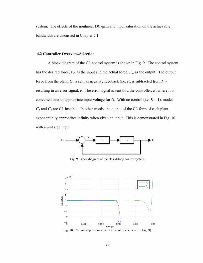
A block diagram of the CL control system is shown in Fig. 9. The control system

has the desired force, Fd, as the input and the actual force, Fa, as the output. The output

force from the plant, G, is sent as negative feedback (i.e. Fa is subtracted from Fd)

resulting in an error signal, e. The error signal is sent thru the controller, K, where it is

converted into an appropriate input voltage for G. With no control (i.e. K = 1), models

G3 and G4 are CL instable. In other words, the output of the CL form of each plant

exponentially approaches infinity when given an input. This is demonstrated in Fig. 10

with a unit step input.

Fig. 9. Block diagram of the closed-loop control system.

Fig. 10. CL unit step response with no control (i.e. K =1 in Fig. 9).

0 0.002 0.004 0.006 0.008 0.01!4

!3

!2

!1

0

1

2

3

4x 10

17

Time (s)

Magnitude

G3

G4

Student Version of MATLAB

24

Four different controllers will be considered to improve the performance of the CL

system. The controllers include a Proportional (P) controller, a Proportional-Integral-

Derivative (PID) controller, and two separate H∞ controllers. A P controller, KP, is the

simplest type of controller that can be used for adjusting the input signal to a dynamic

system. It works by modifying the error signal, e, in Fig. 9 by a factor (i.e. KP is a

constant). For simplicity, consider the classic 2nd order system with a natural frequency,

ωn, and damping ratio, ζ. The error signal for a P controlled 2nd-order system is

represented by

�

e =ωn2Fd

ωn2 + KP

. (6)

From this equation, the steady-state (SS) error of the system is found to be non-zero,

which is an undesirable characteristic in control design. Increasing KP will reduce the SS

error; however, doing so will affect other system dynamics including the un-damped

natural frequency and damping ratio [1].

The PID controller is expressed in the form

�

KPID = KP 1+1KI s

+ KDs⎛ ⎝ ⎜

⎞ ⎠ ⎟ , (7)

where KI and KD are the integral and derivative controller gains, respectively. The

dynamics of the error signal for a PID controlled 2nd-order system are defined as

�

˙ ̇ e +ωn

2 + KP

2ζωn + KD

˙ e +KI

2ζωn + KD

e = 0 . (8)

For a system at SS, the derivatives of the error,

�

˙ ̇ e and

�

˙ e , go to zero. As a result, the error,

e, also goes to zero for a PID control system. Tuning a PID controller can be difficult

given that gains KP, KI, and KD have competing effects on the response of the system.

25

When defining time domain performance, the proportional gain KP is used to reduce the

percent overshoot, the integral gain KI is used to reduce rise time, and the derivative gain

KD is used to increase stability of the system [1]. A balance between each gain is needed

to achieve the desired performance requirements. Controller gains of KP = 1.2e-3, KI =

3.0e-3, and KD = 2.5e-2 are found to provide models G3 and G4 with the best overall CL

performance (both the P and PID control systems use these gain values).

To increase the robustness of a control system (i.e. increase the ability of the

control system to adjust to uncertainties), H∞ loop-shaping design is performed to find a

controller that optimally robustifies a shaped plant. A shaped plant is a linear model

multiplied by some type of controller. For example, a model G and controller K can be

combined into the shaped plant KG. The controller within the shaped plant “determines

such overall characteristics as response speed, damping characteristics, and steady-state

error” of the CL system, while the H∞ controller is used to compensate for uncertainties

[6]. Through the loop shaping procedure, the H∞ controller, KH, is defined as

�

KH =A + BF + γ 2(LT )−1ZCT (C + DF)

BT Xγ 2(LT )−1ZCT

−DT

⎡

⎣ ⎢

⎤

⎦ ⎥ (9)

�

F = −S−1(DTC + BT X) (10)

�

L = (1− γ 2)I + XZ , (11)

where A, B, C, D is the state-space representation of the shaped plant, Z and X are unique

positive definite solutions to the Riccati equations

�

(A − BS−1DTC)Z + Z(A − BS−1DTC)T − ZCTR−1CZ + BS−1BT = 0 (12)

�

(A − BS−1DTC)T X + X(A − BS−1DTC) − XBTS−1BT X + CTR−1C = 0 (13)

and

26

�

γ > γ min = (1+ ρs(XZ))1/ 2, (14)

where ρs is the spectral radius (maximum singular value) of the shaped plant [5]. The

Matlab® M-file coprimeunc given by [5] uses the robust control toolbox along with Eqs.

(9-14) in obtaining an optimal H∞ controller for a given shaped plant. Controller KPID

and the linear models G3 and G4 are used in finding two separate H∞ controllers (i.e.

KPIDG3 and KPIDG4 are the shaped plants from which the H∞ controllers are designed).

The controllers are given as

�

KH 3 =229.7s2 +1.334e5s + 6.305e6

s3 + 972.4s2 + 3.579e5s +1.49e7 (15)

and

�

KH 4 =231.9s2 + 7.484e4s + 9.687e6

s3 + 601.7s2 +1.993e5s + 2.068e7, (16)

where KH3 is the H∞ controller found from the shaped plant KPIDG3 (shaped plant

containing the 3rd order model) and KH4 is the H∞ controller found from the shaped plant

KPIDG4 (shaped plant containing the 4th order model).

The robustifying characteristics of the H∞ controllers can be observed by

comparing the OL frequency response of the shaped plants, KPIDG3 and KPIDG4, with the

OL response of the shaped plants with H∞ control, KH3KPIDG3 and KH4KPIDG4 (see Fig.

11). The crossover frequency (i.e. the frequency at which the magnitude of the OL

response crosses 0 dB) and the phase lag at the crossover frequency for each OL response

is given in Table 2. A large OL crossover frequency is representative of a system with a

large CL bandwidth frequency, and vice-versa. A system with a large bandwidth has

better performance, while a system with a small bandwidth has increased

robustness/stability [5]. The OL phase lag at the crossover frequency also gives insight

27

into the CL stability of the control system. The closer the phase lag is to 180 degrees, the

closer the system is to instability [5]. Given these definitions along with the data in Table

2, the PID controller is expected to provide better CL performance, and the H∞

controllers are expected to increase the robustness of the system. The CL performance

and stability of each control system is discussed in detail in Chapters 5 and 6.

Table 2. Crossover frequencies and corresponding phase lags for the shaped plants and shaped plants with H∞ control.

Crossover Freq. (Hz) Phase at Crossover Freq. (deg) KPIDG3 28.1 128.8 KH3KPIDG3 11.9 109.8 KPIDG4 25.6 125.5 KH4KPIDG4 11.3 107.4

Fig. 11. OL frequency response of the shaped plants and shaped plants with H∞ control.

10!1

100

101

102

!40

!30

!20

!10

0

10

20

30

40

50

Frequency (Hz)

Ma

gn

itu

de

(d

B)

KPID

G3

H3K

PIDG

3

KPID

G4

H4K

PIDG

4

10!1

100

101

102

!260

!240

!220

!200

!180

!160

!140

!120

!100

!80

Frequency (Hz)

Ph

ase

(d

eg

)

Student Version of MATLAB

28

Chapter 5.

CLOSED-LOOP PERFORMANCE

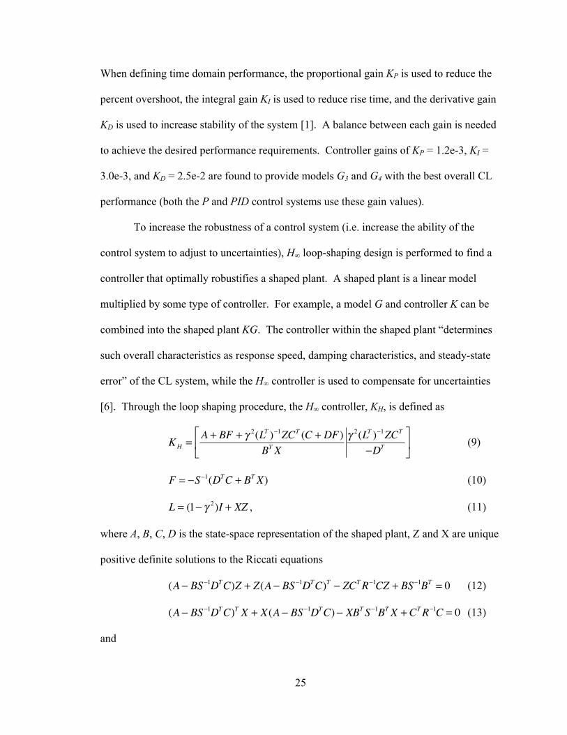
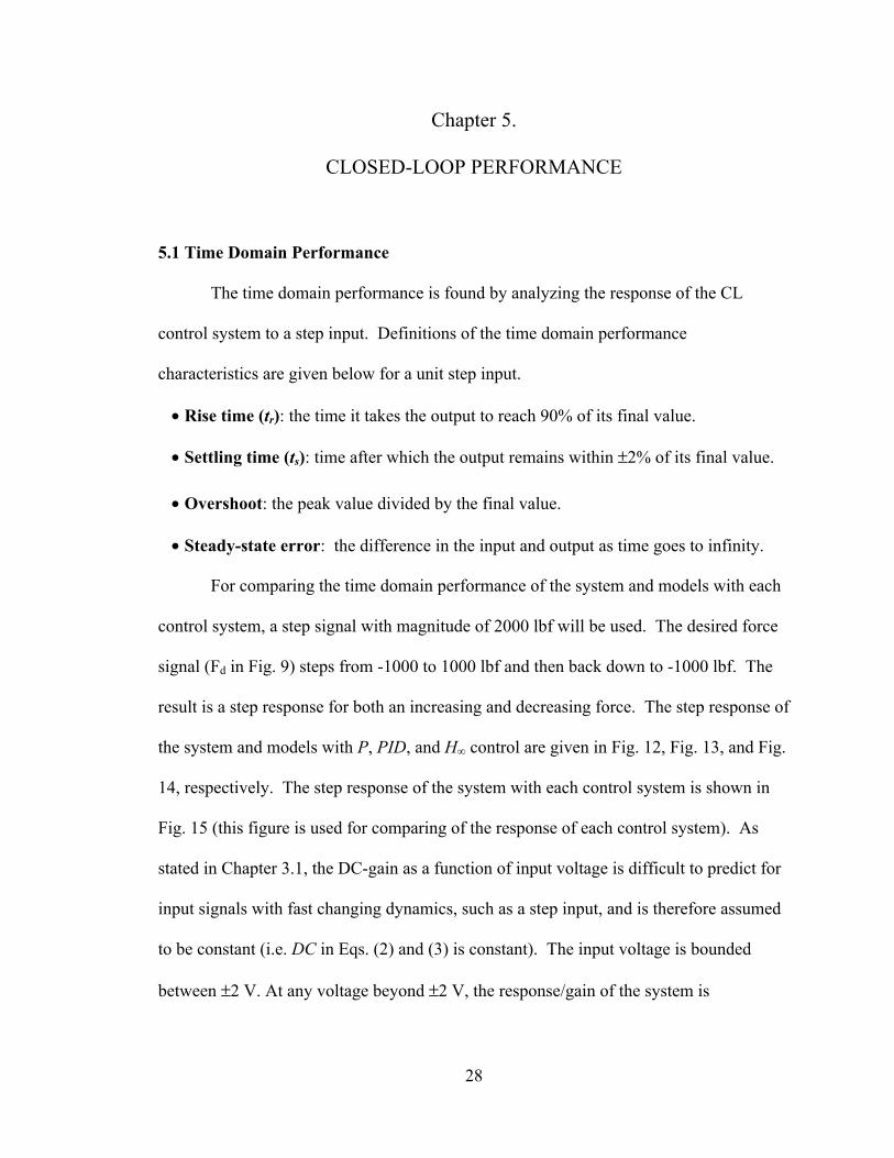
5.1 Time Domain Performance

The time domain performance is found by analyzing the response of the CL

control system to a step input. Definitions of the time domain performance

characteristics are given below for a unit step input.

• Rise time (tr): the time it takes the output to reach 90% of its final value.

• Settling time (ts): time after which the output remains within ±2% of its final value.

• Overshoot: the peak value divided by the final value.

• Steady-state error: the difference in the input and output as time goes to infinity.

For comparing the time domain performance of the system and models with each

control system, a step signal with magnitude of 2000 lbf will be used. The desired force

signal (Fd in Fig. 9) steps from -1000 to 1000 lbf and then back down to -1000 lbf. The

result is a step response for both an increasing and decreasing force. The step response of

the system and models with P, PID, and H∞ control are given in Fig. 12, Fig. 13, and Fig.

14, respectively. The step response of the system with each control system is shown in

Fig. 15 (this figure is used for comparing of the response of each control system). As

stated in Chapter 3.1, the DC-gain as a function of input voltage is difficult to predict for

input signals with fast changing dynamics, such as a step input, and is therefore assumed

to be constant (i.e. DC in Eqs. (2) and (3) is constant). The input voltage is bounded

between ±2 V. At any voltage beyond ±2 V, the response/gain of the system is

29

considered insignificant (see Chapter 3.3). It is found that a DC-gain of 3100 lbf is a

reasonable approximation for the step input given above.

 

 Fig. 12. CL response of the P control systems with a reference step input from -1000 to

1000 lbf (top) and 1000 to -1000 lbf (bottom).

Fig. 13. CL response of the PID control system with a reference step input from -1000 to

1000 lbf (top) and 1000 to -1000 lbf (bottom).

0 0.05 0.1 0.15500

600

700

800

900

1000

1100

1200

Time (s)

Forc

e (

lbf)

System ResponceG

3 (DC = 3100)

G4 (DC = 3100)

0 0.05 0.1 0.15

!1200

!1100

!1000

!900

!800

!700

!600

!500

Time (s)

Forc

e (

lbf)

Student Version of MATLAB

0 0.05 0.1 0.15500

1000

1500

Time (s)

Forc

e (

lbf)

System ResponceG

3 (DC = 3100)

G4 (DC = 3100)

0 0.05 0.1 0.15!1500

!1000

!500

Time (s)

Forc

e (

lbf)

Student Version of MATLAB

30

Fig. 14. CL response of the H∞ control systems with a reference step input from -1000 to

1000 lbf (top) and 1000 to -1000 lbf (bottom).

Fig. 15. CL response of the system with a reference step input from -1000 to 1000 lbf

(top) and 1000 to -1000 lbf (bottom).

The system and models have an under-damped oscillatory response with SS error

when controller KP is used (see Fig. 12). When comparing the response of the system

and models, the settling time of the system is much faster. In addition, the system has a

faster rise time when the input signal steps down from 1000 to -1000 lbf. Models G3 and

0 0.05 0.1 0.15 0.2 0.25500

600

700

800

900

1000

Time (s)

Fo

rce

(lb

f)

System Responce w/ KH3

System Responce w/ KH4

G3 (DC = 3100)

G4 (DC = 3100)

0 0.05 0.1 0.15 0.2 0.25

!1000

!900

!800

!700

!600

!500

Time (s)

Fo

rce

(lb

f)

Student Version of MATLAB

0 0.05 0.1 0.15!1000

!500

0

500

1000

1500

Time (s)

Forc

e (

lbf)

KP

KPID

KH3

KH4

0 0.05 0.1 0.15!1500

!1000

!500

0

500

1000

Time (s)

Forc

e (

lbf)

Student Version of MATLAB

31

G4 also differ slightly from one another. Model G4 has less of an overshoot, while G3 has

a faster rise time. Both models have similar settling times. The response of the system

and models with controller KPID is also under-damped with an increase in overshoot;

however, there is little-to-no oscillation and zero SS error (see Fig. 13). Both the rise

time and overshoot of the system are smaller than either model, yet the settling times are

very similar for all cases. Models G3 and G4 differ in similar ways as they did for the P

controlled step response. When the H∞ controllers, KH3 and KH4, are used (see Fig. 14),

the response of the system and models has zero SS error and very little

overshoot/oscillation (i.e. the damping ratio is close to 1). The system is found to have a

much larger settling time and slightly larger overshoot than either model. The system

and model G4 are slightly under-damped (small overshoot), while model G3 is over-

damped (zero overshoot). Given that the H∞ controllers are designed specifically for G3

and G4 (i.e. KH3 is designed for G3 and KH4 is designed for G4), KH3 is not be used to

control G4 nor is KH4 used to control G3.

The variations between the time domain response of the system and models

described above are mainly due to the assumption of a constant DC-gain. In reality, the

gain of the system is continually changing as the input voltage to the servo-valve

amplifier changes, which will change the response of the system (this is a non-linear trait

of the system). The time domain performance characteristics for all step response data

are given in Table 3. The system has a small rise time, settling time, and overshoot with

KP as the control system; however, the SS error associated with P control is a major

drawback. Using KPID reduces the rise time and eliminates the SS error, but the settling

time and overshoot are increased significantly. The H∞ controllers also eliminate SS error

32

and have much smaller overshoots than the other control systems. Then again, they also

have the largest rise time and settling time. The frequency domain performance can now

be found to more fully understand the performance characteristics of each control system.

Table 3. Time domain performance for system and models. Rise Time

(ms) Settling Time

(ms) Overshoot

(%) SS error

(%) System 17.1 56.4 6.1 10.6

G3 16.6 71.3 9.8 10.6 P Control (KP) G4 16.5 89.0 13.1 10.6

System 15.8 89.1 19.7 0 G3 18.4 80.8 22.8 0 PID Control

(KPID) G4 18.7 82.1 21.6 0 System w/ KH3 18.6 96.1 1.9 0 System w/ KH4 17.8 91.7 2.2 0

G3 w/ KH3 26.6 44.8 0 0 H∞ Control

(KH3 and KH4) G4 w/ KH4 24.4 34.2 0.8 0

5.2 Frequency Domain Performance

The frequency domain performance is characterized via the CL bandwidth

frequency, ωB, of the system. The bandwidth of a system is the frequency range over

which control is effective, and the maximum frequency in this range is called ωB. The

bandwidth frequency is very important for understanding the “benefits and trade-offs” for

a given feedback control system [5]. Large bandwidths usually correspond to a faster

response (i.e. faster rise times and settling times) since high-frequency input signals are

more easily passed on to the outputs of the system. Consequently, systems with large

bandwidths are also more susceptible to noise or uncertainties in the system. Small

bandwidths correspond to a slower response with an increased ability to adjust to

uncertainty (i.e. an increased robustness). The CL ωB is defined as the frequency at

which the Bode magnitude plot of the system decreases by 3 dB (the magnitude at low

33

frequencies is considered the reference frequency). As the magnitude decreases by more

than 3 dB, feedback is no longer effective in improving the performance of the system

[5].

The control systems found in Chapter 4.2 are designed using the linear TF’s found

from the OL chirp signal data in Chapter 3.2, more precisely trial (b), which corresponds

to an input chirp signal of magnitude 0.5 V and offset of 0 V. The OL response to this

chirp signal is shown in Fig. 16 (a time interval of 10 seconds and frequency range of 50

Hz is used). At low frequencies, the OL chirp signal results in a force output magnitude

of approximately 1850 lbf at an offset of -400 lbf. To have an accurate comparison of the

OL and CL systems, the desired force signal (chirp signal) for each CL control system

will have a magnitude and offset equal to the low frequency OL output (i.e. Fd in Fig. 9 is

set as a chirp signal with magnitude of 1850 lbf and offset of -400 lbf). Bode magnitude

and phase plots for each CL control system can be found through the same process

outlined in Chapter 3.1 for the OL system. For easy comparison to the CL control cases,

the OL Bode magnitude response is normalized (i.e. the magnitude response is divided by

the low frequency gain found from Fig. 6). The full input range of the system (-2 to 2 V)

is used in analyzing the CL frequency domain performance to give an overall increase in

system performance. The magnitude and phase lag of the normalized OL and CL control

cases over a frequency range of 50 Hz are given in Fig. 17 and Fig. 18, respectively. The

resulting bandwidth frequencies of the system and models are given in Table 4.

34

Fig. 16. Open-loop response to a chirp signal with magnitude of 0.5 V, offset of 0 V, and

frequency range from 0 to 50 Hz.

Fig. 17. Bode magnitude plot of the normalized OL and CL P control (top), PID control

(middle), and H∞ control (bottom) cases.

0 1 2 3 4 5 6 7 8 9 10!2500

!2000

!1500

!1000

!500

0

500

1000

1500

2000

Time (s)

Fo

rce

(lb

f)

DC!gain = 3700 lbf/V

Student Version of MATLAB

100

101

!20

!15

!10

!5

0

5

Frequency (Hz)

Magnitude (

dB

)

System ! OL (Normalized)

System ! CL w/ KP

G3 ! CL w/ K

P

G4 ! CL w/ K

P

100

101

!20

!15

!10

!5

0

5

Frequency (Hz)

Magnitude (

dB

)

System ! OL (Normalized)

System ! CL w/ KPID

G3 ! CL w/ K

PID

G4 ! CL w/ K

PID

100

101

!20

!15

!10

!5

0

5

Frequency (Hz)

Magnitude (

dB

)

System ! OL (Normalized)

System ! CL w/ H3

System ! CL w/ H4

G3 ! CL w/ H

3

G4 ! CL w/ H

4

Student Version of MATLAB

35

Fig. 18. Bode phase plot of the normalized OL and CL P control (top), PID control

(middle), and H∞ control (bottom) cases.

As shown in Fig. 17, the CL magnitude response of the system and model G4

have very similar slopes at higher frequencies, which is most evident with P and PID

control. The CL magnitude response of model G3 has a smaller slope at higher

frequencies due to the inaccuracy of the 3rd-order model in the OL magnitude response

(see Fig. 6). The phase plots of the system and models (shown in Fig. 18) all have

similar slopes at higher frequencies due to the OL phase accuracy of both models (see

Fig. 7). The main differences between the frequency domain response of the system and

models are the resonant frequencies for the magnitude (i.e. the frequency at which the

100

101

!200

!150

!100

!50

0

Frequency (Hz)P

ha

se

(d

eg

)

System ! OL

System ! CL w/ KP

G3 ! CL w/ K

P

G4 ! CL w/ K

P

100

101

!200

!150

!100

!50

0

Frequency (Hz)

Ph

ase

(d

eg

)

System ! OL

System ! CL w/ KPID

G3 ! CL w/ K

PID

G4 ! CL w/ K

PID

100

101

!200

!150

!100

!50

0

Frequency (Hz)

Ph

ase

(d

eg

)

System ! OL

System ! CL w/ H3

System ! CL w/ H4

G3 ! CL w/ H

3

G4 ! CL w/ H

4

Student Version of MATLAB

36

system oscillates at a maximum amplitude) and the drop-off frequencies for the phase

(i.e. the frequency at which the phase begins to decrease at an accelerated rate). Both the

resonance and drop-off frequencies are smaller for the models than they are for the

system. These differences can once again be attributed to the assumption of a constant

DC-gain. In fact, the gain of the system is continually changing as the frequency and

magnitude of the input voltage to the servo-valve amplifier changes (the gain changes

with magnitude due to the gain nonlinearities).

As shown in Table 4, the servo system has bandwidths from largest to smallest

with controllers KP, KPID, KH4, and KH4, respectively. Therefore, controller KP and KPID

provide the system with a faster response (better performance), which corresponds to

faster rise times in the time domain (see Table 3). In contrast, controllers KH4 and KH4

increase the stability of the system (better robustness), which corresponds to small

overshoots in the time domain. The saturation frequency of the system and models (i.e.

the frequency at which the input voltage reaches ±2 V) is also noted in Table 4 for each

CL control system. Decreasing the magnitude of the CL chirp signal (desired force

signal) will decrease the amount of saturation the system experiences. However, for sake

of comparing the OL and CL responses, reducing the CL chirp magnitude requires an OL

response with a smaller output force magnitude (i.e. the OL chirp input voltage

magnitude must be reduced).

The only controller that does not cause the system to saturate is KH3, which is also

the controller that results in the smallest CL bandwidth. Control systems with small

bandwidths do not have the tendency to amplify the error signal as much as higher

bandwidth systems (i.e. they are less likely to saturate as the error signal increases in

37

magnitude). The input voltage to the servo-valve amplifier for CL control with KH3 and

KH4 is shown in Fig. 19. Controller KH3 keeps the input voltage to the servo-valve

amplifier within ±1.7 V over the entire frequency range; however, controller KH3

saturates at approximately 6.2 seconds (33.3 Hz) and remains saturated as the frequency

of the chirp signal continues to increase. Nevertheless, limiting the system between ±2 V

does not affect the performance of the system as much as one might think. As discussed

in Chapter 3.3, the DC-gain of the system gets very small as the input voltage reaches ±2

V. This means that the system does not produce a significant response beyond ±2 V. In

other words, the response of the system when given an input of 2 V is nearly the same as

the response when given an input of 5 V (5 V is the maximum operating voltage of the

servo-valve amplifier as specified by the manufacture). Limiting the input voltage by any

more that ±2 V will, however, begin to have an effect on the performance of the system.

Table 4. Bandwidth frequencies for the OL and CL frequency response and

corresponding saturation frequencies. OL CL w/ KP CL w/ KPID CL w/ KH3 CL w/ KH4

System 6.9 46.4 40.5 28.2 38.1 G3 8.5 46.8 41.1 26.6 - Bandwidth Freq. (Hz) G4 7.8 38.1 34.4 - 25.9

System - 32.5 15.1 >50 33.3 G3 - 21.3 21.2 >50 - Saturation Freq. (Hz) G4 - 20.8 21.3 - 34.1

38

Fig. 19. Input voltage to the servo-valve amplifier for CL control with KH# (top) and KH#

(bottom).

0 1 2 3 4 5 6 7 8 9 10!2

!1

0

1

2

Time (s)

Input V

oltage (

V)

0 1 2 3 4 5 6 7 8 9 10!3

!2

!1

0

1

2

3

Time (s)

Input V

oltage (

V)

No Saturation

Saturation at 2 volts

Saturation at !2 volts

Student Version of MATLAB

39

Chapter 6

NOMINAL/ROBUST STABILITY AND PERFORMANCE

6.1 Dynamic and Parametric Uncertainties

The basic requirement of CL control systems is to achieve a certain level of

performance along with the ability to tolerate uncertainties within the system. The

performance levels involve such things as “command following, disturbance rejection,

[and] sensitivity,” while the uncertainty tolerances deal with the “inevitable differences

which exist between the physical plant and its mathematical […] model” [7]. Therefore,

in order to fully understand a CL control system, it is important to analyze the robustness

of the stability and performance characteristics with respect to all plant perturbations [8].

To characterize the stability and performance of each control system, the

uncertainties in the system must first be defined. There are two main uncertainties that

exist in the servo system: a dynamic (frequency-dependent) uncertainty in the

experimental chirp data and a parametric (real) uncertainty in the DC-gain. The dynamic

uncertainty is represented as a multiplicative uncertainty (MU) of the form

�

Gp,d = Gn (1+ wIΔI ) ,

�

ΔI ( jω) ≤ 1

�

∀ω (17)

where Gp,d is the dynamically perturbed plant (i.e. the experimental chirp data), Gn is the

nominal plant (i.e. the TF model of the system), wI is a TF used in modeling the dynamic

uncertainty, ΔI is any stable TF such that

�

ΔI ∞≤ 1, and ω is the frequency. The dynamic

uncertainty TF, wI, is found from the relationships

�

lI (ω) = maxG∈Π

Gp,d ( jω) −Gn ( jω)Gn ( jω)

(18)

40

and

�

wI ( jω) ≥ lI (ω) ,

�

∀ω , (19)

where lI is the maximum MU from the chirp data. Since the 4th order model G4 matches

the experimental OL chirp data over the entire frequency range (0 to 100 Hz) it will

represent the nominal plant. The MU uncertainty from each chirp signal (trial (a-c)) is

shown in Fig. 20. As defined in Eq. (19), the magnitude of wI must be greater than or

equal to lI over all frequencies (i.e. wI represents the least upper bound of dynamic

uncertainty over the entire frequency range). The fitmag command in Matlab®, which fits

a stable TF with minimum phase to a set of magnitude data points, is used in finding a

3rd-order TF, wI, that bounds all dynamic uncertainties associated with the experimental

chirp data (see Fig. 20). The TF form of wI is defined as

�

wI =8.892s3 + 7825s2 + 6.49e6s +1.304e9s3 + 5254s2 +1.553e6s + 2.231e9

. (20)

Fig. 20. Dynamic MU for trials (a-c) and resulting uncertainty TF.

10!1

100

101

102

10!2

10!1

100

Frequency (Hz)

Ma

gn

itu

de

MU for trial (c)

MU for trial (b)

MU for trial (a)Dynamic Uncertainty TF (w

I)

Student Version of MATLAB

41

The parametric gain uncertainty in MU form is written as

�

Gp,p = Gn (1+ rkΔ) ,

�

Δ ≤ 1, (21)

where Gp,p is the parametrically perturbed plant, Δ is a real scalar, and rk is the relative

magnitude of the gain uncertainty defined by

�

rk =(kmax − kmin )(kmax + kmin )

, (22)

where kmax and kmin are the maximum and minimum gain values, respectively. As shown

in Chapter 3.3, the input voltage range affects the minimum and maximum DC-gain of

the system. Three separate input voltage ranges (±2, ±1, and ±0.5 V) are used to show

how changing the input range influences the robust stability/performance of the control

systems. Referring to polynomial dPt in Fig. 8, input ranges of ±2, ±1, and ±0.5 V result

in minimum/maximum gains of 0/4250, 1930/4250, and 3420/4135 lbf/V, respectively.

Therefore, the relative gain uncertainty magnitude, rk, for the respective input ranges is 1

(100%), 0.379 (37.9%), and 0.095 (9.5%). Reducing the input range reduces the amount

of parametric uncertainty; however, doing so will limit the performance of the system.

6.2 Performance Weight

A block diagram of the servo system with both dynamic and parametric

uncertainties is shown in Fig. 21 (Gp is the plant perturbed by both dynamic and

parametric uncertainties). To analyze the performance of the system, a performance

weight TF, wP, is also needed. The performance weight is written as

�

wP =s /M + ωBR

s + ωBRA, (23)

42

where M is the allowable error at high frequencies, A is the allowable error at low

frequencies, and ωBR is the approximate bandwidth requirement. The inverse of wP

(shown in Fig. 22 for A = 0.1, M = 3, and ωBR = 5 Hz) represents the upper bound of the

sensitivity, |S|. The sensitivity function, S, is the TF between the reference input and

error in Fig. 21 given as

�

S =1

1+ GpK.

(24)

In order for the system to meet the performance requirements defined by wP, the

H∞ norm of the weighted sensitivity function, wPS, must be less than 1 (alternatively, |S|

must be less than

�

1/wP ( jω) to maintain performance) [5]. Referring to Fig. 22, it is

shown that

�

1/wP ( jω) is equal to A (0.1) at low frequencies and M (3) at high

frequencies. If A and M are left constant, increasing or decreasing ωBR will affect how

much error is allowed at lower frequencies. Since wP is a 1st-order TF, the slope of

�

1/wP ( jω) will not change. As a result, changing the value of ωBR will simply slide the

graph in Fig. 22 to the left for smaller ωBR values and to the right for larger ωBR values.

Therefore, small and large values of ωBR will increase and decrease the allowable error at

lower frequencies, respectively. A CL system that is capable of maintaining performance

at the largest possible value of ωBR, which correlates to a system that is able to accurately

track higher frequency input signals, is desired. In regards to the servo system, locating

wP on the error signal (see block diagram in Fig. 21) allows the performance of the

system to be gauged by the difference between desired force input and actual force

output. The error signal is fed through the wP block and a fictitious uncertainty block, ΔP,

43

before it is sent back to the input of the system (see Fig. 21). If the magnitude of the

error signal is larger than

�

1/wP ( jω) at a given ω, the servo system does not maintain the

specified performance requirements.

Fig. 21. CL system with multiplicative uncertainties and performance measured at the

error.

Fig. 22. Inverse of the performance weight (i.e. 1/| wP(jω)|)

6.3 Obtaining P and N Matrixes

The Block diagram in Fig. 21 can now be analyzed to obtain the generalized plant

model P. The generalized plant (shown in matrix form in Fig. 23) contains Gn, wI, rk, wP,

and the interconnection structure between the plant and the controller K [5]. Referring to

10!1

100

101

102

10!1

100

Frequency (Hz)

Ma

gn

itu

de

!BR

= 5 Hz

M = 3

A = 0.1

Student Version of MATLAB

44

Fig. 21, plant P has uΔ, uΔI, uΔP, and v as inputs and yΔ, yΔI, yΔP, and u as outputs. The

matrix form of P is defined by

�

uΔuΔIuΔPv

⎧

⎨ ⎪ ⎪

⎩ ⎪ ⎪

⎫

⎬ ⎪ ⎪

⎭ ⎪ ⎪

= P[ ]

yΔyΔIyΔPu

⎧

⎨ ⎪ ⎪

⎩ ⎪ ⎪

⎫

⎬ ⎪ ⎪

⎭ ⎪ ⎪

(25)

�

P =

0 0 0 rkwI 0 0 wI

−wPGn −wPGn wP −wPGn

−Gn −Gn 1 −Gn

⎡

⎣

⎢ ⎢ ⎢ ⎢

⎤

⎦

⎥ ⎥ ⎥ ⎥

, (26)

Fig. 23. P and N matrixes.

As shown in Fig. 23, the P-matrix is partitioned into 4 elements (P11, P12, P21, and

P22). The column partition corresponds to the number of exogenous inputs from the

uncertainty Δ-matrix and the row partition corresponds to the number of endogenous

outputs to the uncertainty Δ-matrix. That is to say, P11 has dimensions a×b, where a and

b are the number of outputs and inputs of the Δ-matrix, respectively. The partitioned

elements of P are

45

�

P11 =0 0 0wI 0 0

−wPGn −wPGn wP

⎡

⎣

⎢ ⎢ ⎢

⎤

⎦

⎥ ⎥ ⎥

�

P12 =rkwI

−wPGn

⎡

⎣

⎢ ⎢ ⎢

⎤

⎦

⎥ ⎥ ⎥ (27)

�

P21 = −Gn −Gn 1[ ]

�

P22 = −Gn[ ]. (28)

The controller K can be absorbed into the interconnection structure to obtain the

system N. In other words, N is found by using K to close the lower feedback loop around

P (see Fig. 23). The equation used in finding the N-matrix from the partitioned P-matrix

and controller K is presented below (this is referred to as the lower linear fractional

transformation).

�

N = P11 + P12K(I − P22K)−1P21 (29)

The N-matrix has the same dimension as P11 (i.e. 3×3). Similar to the P-matrix, the N-

matrix is partitioned into 4 elements (N11, N12, N21, and N22). Element N11 has dimensions

i×j, where i and j are the respective number of outputs and inputs of the parametric, Δ,

and dynamic, ΔI, uncertainty blocks in the Δ-matrix (N11 is 2×2). In contrast, element N22

has dimension k×w, where k and w are the respective number of performance outputs and

inputs of the performance uncertainty block, ΔP, in the Δ-matrix (N22 is 1x1). Therefore,

element N11 contains information regarding the uncertainties of the system (i.e. rk and wI),

while element N22 contains the performance requirements of the system (i.e. wP). The off

diagonal elements N12 and N21 may contain uncertainty and/or performance information.

The N matrix can now be used in determining the stability and performance of the

system.

46

6.4 Defining Stability/Performance and the Structured Singular Value

The definitions of nominal/robust stability and performance are given below.

• Nominal stability (NS): The system (i.e. nominal model) is stable with no

uncertainty. NS ⇔ N is internally stable (i.e. all eigenvalues of N are in the left half

plane (LHP)) [5].

• Robust stability (RS): The system is stable for all perturbed plants about the nominal

model up to a worst-case model uncertainty. RS ⇔ NS and

�

µΔ (N11(ω)) < 1 ∀ω,

where µ is the structured singular value (SSV) and subscript

�

Δ is the structured 2×2

uncertainty matrix that includes Δ and Δ1 (

�

Δ is diagonal is structure) [5].

• Nominal performance (NP): The system (i.e. nominal model) satisfies the

performance specification with no uncertainty. NP ⇔ NS and

�

σ (N22(ω)) < 1 ∀ω [5],

where

�

σ is the maximum singular value of the TF.

• Robust performance (RP): The system satisfies the performance specifications for

all perturbed plants about the nominal plant up to the worst-case model uncertainty.

RP ⇔ NS and

�

µ ˆ Δ (N(ω)) < 1 ∀ω , where subscript

�

ˆ Δ is the structured 3×3 uncertainty

matrix that includes Δ, Δ1, and ΔP (

�

ˆ Δ is diagonal in structure) [5].

The SSV, µ, is a generalization of

�

σ and ρs [5]. In this structure, parametric

uncertainties are handled by replacing them with complex parameters when the singular

value is used [8]. Doyle [9] first introduced the SSV in 1982 as a way of “dealing with

problems of robust stability with respect to […] uncertainty in situations where it is

necessary to exploit the structure of the problem to get less conservative conditions” [10].

In other words, the SSV of a complex system is less than or equal to the maximum

47

singular value of that system. Therefore, defining stability and performance using

�

σ

instead of µ results in a more conservative result. The conservative nature of using

�

σ in

performing robust analysis on a hydraulic servo system is discussed in detail by [11].

The structured singular value of a complex matrix L is defined by [9] as

�

µ(L) = (min{σ (Δ) | det(I + LΔ) = 0})−1 (30)

where Δ denotes a set of complex matrices with

�

σ (Δ) ≤ 1. If no structure Δ exists, µ(L) =

0 [10]. If the structure Δ is 1×1 (i.e. L is a single TF),

�

µ(L) = σ (L) (this relationship is

used in defining NP since N22 is a 1×1 TF matrix). A value of µ = 1 signifies that there

exists a perturbation just large enough to make I + LΔ singular (feedback is no longer

considered effective when µ > 1). A larger value of µ (say 0.99) requires only a smaller

perturbation to make I + LΔ singular; therefore, smaller values of µ are desired [5]. An

algorithm by [12] dating back to 1986 uses “several smooth optimization problems” to

solve for µ. For simplicity, the Matlab® command ssv is used for all SSV calculations.

6.5 Nominal and Robust Stability

The stability of the servo system is tested for input voltage ranges of ±2 V (rk =

1), ±1 V (rk = 0.379), and ±0.5 V (rk = 0.095). The N-matrix for each control system has

eigenvalues in the LHP when rk equals 0.095, 0.379, and 1. Therefore, each controller

provides NS to the CL system for input voltage ranges up to ±2 V. The RS of the control

systems at each value of rk is determined through the structured singular values of N11

over a frequency range from 0 to 100 Hz (see Fig. 24). All controllers are found to

provide RS (i.e.

�

µΔ (N11(ω)) < 1 ∀ω) when rk = 0.095 and rk = 0.379. However, when rk

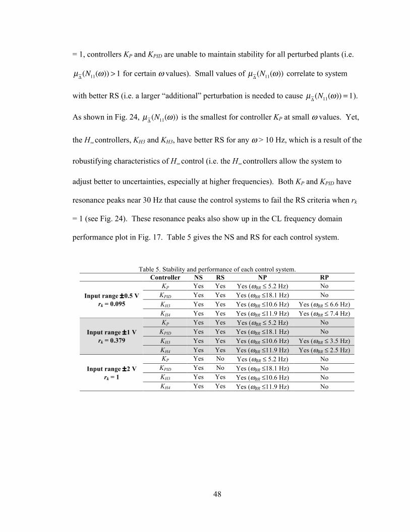
48

= 1, controllers KP and KPID are unable to maintain stability for all perturbed plants (i.e.

�

µΔ (N11(ω)) > 1 for certain ω values). Small values of

�

µΔ (N11(ω)) correlate to system

with better RS (i.e. a larger “additional” perturbation is needed to cause

�

µΔ (N11(ω)) = 1).

As shown in Fig. 24,

�

µΔ (N11(ω)) is the smallest for controller KP at small ω values. Yet,

the H∞ controllers, KH3 and KH3, have better RS for any ω > 10 Hz, which is a result of the

robustifying characteristics of H∞ control (i.e. the H∞ controllers allow the system to

adjust better to uncertainties, especially at higher frequencies). Both KP and KPID have

resonance peaks near 30 Hz that cause the control systems to fail the RS criteria when rk

= 1 (see Fig. 24). These resonance peaks also show up in the CL frequency domain

performance plot in Fig. 17. Table 5 gives the NS and RS for each control system.

Table 5. Stability and performance of each control system.

Controller NS RS NP RP KP Yes Yes Yes (ωBR ≤ 5.2 Hz) No

KPID Yes Yes Yes (ωBR ≤18.1 Hz) No KH3 Yes Yes Yes (ωBR ≤10.6 Hz) Yes (ωBR ≤ 6.6 Hz)

Input range ±0.5 V rk = 0.095

KH4 Yes Yes Yes (ωBR ≤11.9 Hz) Yes (ωBR ≤ 7.4 Hz) KP Yes Yes Yes (ωBR ≤ 5.2 Hz) No

KPID Yes Yes Yes (ωBR ≤18.1 Hz) No KH3 Yes Yes Yes (ωBR ≤10.6 Hz) Yes (ωBR ≤ 3.5 Hz)

Input range ±1 V rk = 0.379

KH4 Yes Yes Yes (ωBR ≤11.9 Hz) Yes (ωBR ≤ 2.5 Hz) KP Yes No Yes (ωBR ≤ 5.2 Hz) No

KPID Yes No Yes (ωBR ≤18.1 Hz) No KH3 Yes Yes Yes (ωBR ≤10.6 Hz) No

Input range ±2 V rk = 1

KH4 Yes Yes Yes (ωBR ≤11.9 Hz) No

49

Fig. 24. Robust stability (i.e.

�

µΔ (N11 (ω )) < 1) for rk = 0.095 (top), rk = 0.379 (middle) and rk = 1 (bottom).

6.6 Nominal and Robust Performance

The performance is also tested for rk = 1, rk = 0.379, and rk = 0.095. To find the

performance of each control system, the performance weight TF, wP, shown in Eq. (23),

must first be defined. Referring to Fig. 21, the performance weight is placed on the error

signal; therefore, the magnitude of the error will determine if the system meets the given

performance requirements. The allowable errors are set at 10% (A = 0.1) for low

frequencies and 300% (M = 3) for high frequencies (the same values of A and M are used

in defining the bandwidth limitation of the system in Chapter 4.1). The performance of

each control system is tested at different values of the ωBR (bandwidth requirement) to

find at what bandwidth the system is considered to have NP and RP.

100

101

102

0

0.05

0.1

0.15

0.2

Frequency (Hz)

µ(N

11)

G

4 w/ K

P

G4 w/ K

PID

G4 w/ K

H3

G4 w/ K

H4

100

101

102

0

0.2

0.4

0.6

0.8

Frequency (Hz)

µ(N

11)

100

101

102

0

0.5

1

1.5

2

Frequency (Hz)

µ(N

11)

rk = 0.095

rk = 0.379

rk = 1

Student Version of MATLAB

50

A control system with NP up to a given bandwidth is able to provide the nominal

plant, Gn, adequate performance (as defined by wP) up to that bandwidth. For example, a

control system that provides Gn with NP up to ωBR = x Hz is able to effectively track a

sine wave at a frequency up to x Hz. The NP (i.e.

�

σ (N22(ω)) ∀ω) for each control

system is illustrated in Fig. 25 for ωBR = 10 Hz. The PID controller is shown to have the

best NP for any ω < 30 Hz, while the H∞ controllers have the best NP for any ω > 30 Hz

(the NP of the H∞ controllers increases as ω increases beyond 5 Hz). The P controller

does not have NP at ωBR = 10 Hz. Once again, KP and KPID have resonance peaks near 30

Hz that have a negative affect on the NP of the system. Table 5 shows the bandwidths

over which each control system maintains NP. Since N22 does not contain any

uncertainty information, each controller has the same NP for the different values of rk.

Controller KPID is able to provide the system with NP over the largest bandwidth (18.1

Hz). Controller KP has the smallest NP range (5.2 Hz) given that the SS error associated

with P control causes the system to exceed the performance requirements at low

frequencies (see Fig. 25). The H∞ controllers have similar NP bandwidths (10 to 11 Hz);

however, controller KH4 is able to maintain NP for a slightly higher value of ωBR.

To qualify as having RP, the structured singular values of the entire N-matrix

must be less than one over all frequencies. A control system with RP up to a given ωBR is

able to provide the perturbed plant, Gp, with adequate performance up to that bandwidth.

Since the N-matrix contains uncertainty and performance information, a system must

have a balance between robustness (good RS) and fast response time (good NP) to

qualify for RP. For this reason, if a given CL control system does not have RS (i.e.

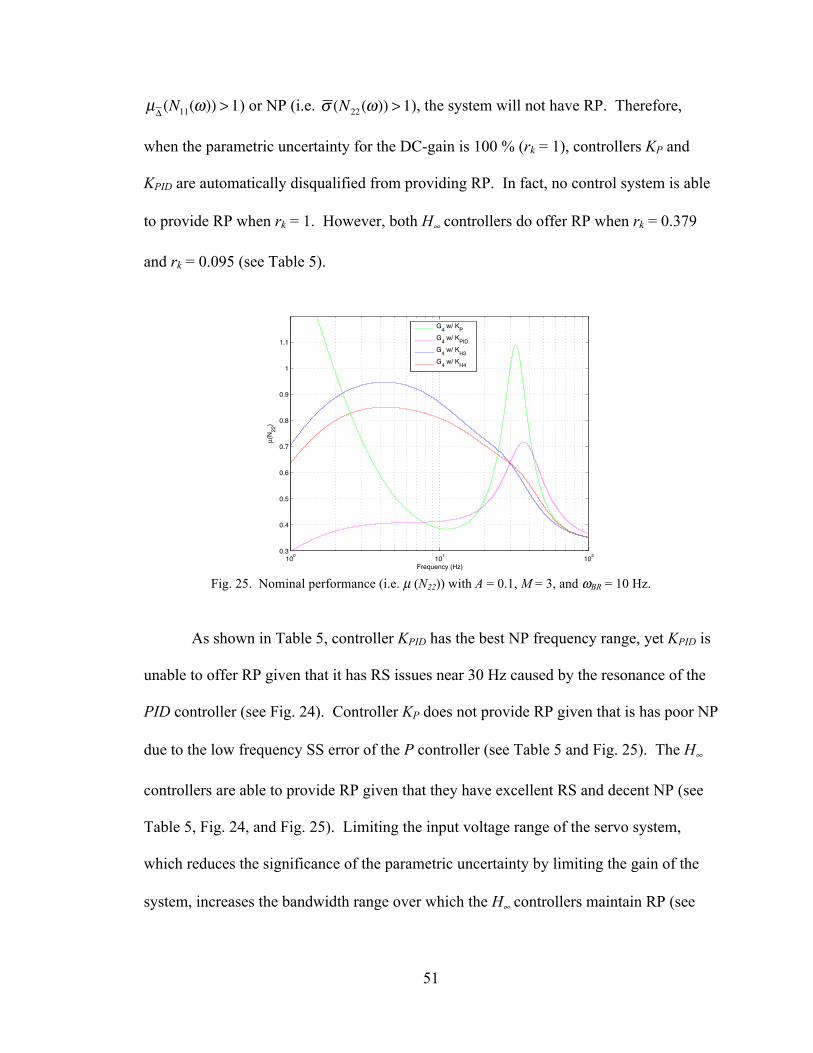
51

�

µΔ (N11(ω)) > 1) or NP (i.e.

�

σ (N22(ω)) > 1), the system will not have RP. Therefore,

when the parametric uncertainty for the DC-gain is 100 % (rk = 1), controllers KP and

KPID are automatically disqualified from providing RP. In fact, no control system is able

to provide RP when rk = 1. However, both H∞ controllers do offer RP when rk = 0.379

and rk = 0.095 (see Table 5).

Fig. 25. Nominal performance (i.e. µ (N22)) with A = 0.1, M = 3, and ωBR = 10 Hz.

As shown in Table 5, controller KPID has the best NP frequency range, yet KPID is

unable to offer RP given that it has RS issues near 30 Hz caused by the resonance of the

PID controller (see Fig. 24). Controller KP does not provide RP given that is has poor NP

due to the low frequency SS error of the P controller (see Table 5 and Fig. 25). The H∞

controllers are able to provide RP given that they have excellent RS and decent NP (see

Table 5, Fig. 24, and Fig. 25). Limiting the input voltage range of the servo system,

which reduces the significance of the parametric uncertainty by limiting the gain of the

system, increases the bandwidth range over which the H∞ controllers maintain RP (see

100

101

102

0.3

0.4

0.5

0.6

0.7

0.8

0.9

1

1.1

Frequency (Hz)

µ(N

22)

G4 w/ K

P

G4 w/ K

PID

G4 w/ K

H3

G4 w/ K

H4

Student Version of MATLAB

52

Table 5). However, by limiting the input voltage, the response of the system will be

restricted causing a reduction in the overall performance of the servo system.

53

Chapter 7.

CONCLUSION

7.1 Experimental Results

The OL response of the hydraulic servo system is best represented as the 4th-order

linear TF model, G4, containing a 1st-order time delay approximation (the 3rd-order TF is

unable to model the system at higher frequencies). The RHP zero associated with the

time delay places a bandwidth limitation,

�

ωB* , of 235 Hz on any feedback control system.

In other words, the CL bandwidth, ωB, of a control system must be less than 235 Hz to

meet the performance requirements of A = 0.1 (10% error at low frequencies) and M = 3

(300% error at high frequencies) (see Eq. (5)). Therefore, there theoretically exists a

controller capable of providing G4 with ωB = 225 Hz (a high order controller is most

likely required to achieve such a bandwidth).

The bandwidth limitation analysis is based on the linear model G4; therefore, it

does not take into account any non-linear behaviors of the real system such as the

deterioration of the DC-gain as the input voltage increases or the saturation of the system.

Furthermore, the OL magnitude response of the system is found to be insignificant at any

frequency greater than 100 Hz (the same cannot be said for the linear model). The actual

�

ωB*

of the non-linear servo system is, therefore, expected to be at some frequency less

than 235 Hz. Of the four controllers designed, the P controller, KP, results in the largest

CL bandwidth of 46.4 Hz, which is much smaller than the linear

�

ωB* . Modifying each

controller (i.e. adjusting controller gains) can further increase the CL bandwidth of the

system; however, doing so may have an adverse affect on the performance and/or

54

robustness of the system. As the overall gain of a controller is increased, the amount of

saturation the system experiences will also increase. When the system saturates, the

effectiveness (i.e. the performance) of the control system is diminished. As a result, the

non-linear characteristics of the servo system cause the actual

�

ωB*

to be significantly less

than what is predicted from the linear model.

When considering time domain performance, KP and KPID provide the system

with the fastest rise times, while KH3 and KH4 result in the least amount of overshoot. The

frequency domain performance results show that controllers KP and KPID provide the

fastest response (i.e. better performance) and controllers KH3 and KH4 as providing the

best stability (i.e. better robustness). Controller KH3 is the only controller that does not

cause saturation when tracking a chirp signal with magnitude of 1850 lbf, offset of -400

lbf, and frequency range of 50 Hz. The ability of a control system to stay within the

active input range of the system (especially at high magnitudes and frequencies) is very

desirable.

Controller KH3 provides the lowest CL bandwidth frequency (28.2 Hz) of any

control system, meaning it is better able to adjust to uncertainties within the system. As a

result of this low bandwidth, the RS (i.e.

�

µΔ (N11(ω)) ) of the KH3 control system has the

smallest magnitude over the majority of the frequency range (see Fig. 24). Controller KP

has the best RS at low frequencies (ω < 10 Hz), but its large resonance peak rear 30 Hz

causes its overall RS to be poor.

Controller KPID offers NP up to a bandwidth of 18.1 Hz, while KH3 and KH4 have

NP up to 10.6 and 11.9 Hz, respectively (the performance weight allows 10% error at low

frequencies and 300% error at high frequencies). These NP results correlate to the

55

frequency domain performance results (i.e. the faster the system can respond, the better

performance it will have). Generally, a higher CL ωB will result in a control system with

better NP. Yet, KP results in the highest CL ωB and poorest NP of all the control systems.

This is due to the SS error associated with P control (i.e. the SS error causes the system to

exceed the low frequency performance criteria at a very small value of ωBR).

In order for the servo system to have RP, the control system must have a balance

between performance and stability. The only controllers capable of providing RP are KH3

and KH4 (see Table 5 for RP data for KH3 and KH4). Controller KH3 provides better RP for

the ±1 V input range (rk = 0.379), while KH4 provides better RP for the ±0.5 V input

range (rk = 0.095). Since decreasing the input range has significant affects on CL

performance, it is desired to have a control system with the best possible performance at

the largest possible input range. Therefore, it is concluded that the best overall control

(i.e. the best balance of CL performance and stability) is attained with KH3.

7.2 Future Work

The force analysis of the system can be investigated further by allowing rod

movement during testing. As shown in Fig. 1, the hydraulic actuator rod (rod A) is

connected to a bracket to eliminate any movement of the actuator rod during loading. To

allow for rod movement, a secondary hydraulic actuator can be used to replace the

bracket. By adding a leakage line and needle valve to the secondary actuator (similar to

what is shown in Fig. 1 for the main loading actuator), the speed at which the actuators

move can be regulated by increasing or decreasing the flow through the secondary

actuator. Increasing the flow rate between the high and low-pressure side of the

56

secondary actuator will cause the actuator to be compressed at a faster rate when

subjected to a load. To overcome the problems of force control caused by actuator

movement, the CL control system (see in Fig. 9) can be modified by adding a correction

to the force demand based on the displacement and/or velocity of the main actuator [4].

Allowing movement in the main actuator rod is beneficial in developing a platform for

testing other actuators. Such a system is outlined by [4] where primary flight actuators

for aircraft are tested by connecting a main loading actuator to a lever arm, which is in

turn connected to a secondary flight actuator. By using a similar setup as outlined by [4],

along with the control design process outlined in this thesis, a control system with the

required performance and robustness can be created for testing a variety of other

hydraulic, pneumatic, or electronic actuators.

Further work can also be conducted to improve the bandwidth/performance of the

control system. Non-linear QFT robust control methodology given by [2], Input-Output

Feedback Linearization given by [3], or a different non-linear approach can be used to

improve the robustness of the servo system by compensating for the non-linear gain

curve shown in Fig. 8. Non-linear procedures are more involved than the linear process

outlined in this thesis, but they should result in a control system that is better able to

compensate for the non-linearities in the servo system and improve upon the overall

performance.

57

BIBLIOGRAPHY

[1] Manring, N. D., 2005, Hydraulic Control Systems, John Wiley & Sons, Hoboken, NJ, 61-64, 156-160, 169-176, 234-252.

[2] Niksefat, N., and Sepehri, N., “Robust Force Controller Design for a Hydraulic

Actuator Based on Experimental Input-Output Data.” IEEE Proc., Vol. 5, Issue 2-4, pp. 3718-3722, 1999.

[3] Chiriboga, J., Thein, M.-W.L., and Misawa, E.A., “Input-Output Feedback

Linearization Control of a Load-Sensing Hydraulic Servo System,” IEEE Proc., pp. 910-915, 1995.

[4] Rito, G. D., Denti E., and Galatolo R., “Robust Force Control in a Hydraulic

Workbench for Flight Actuators,” IEEE Proc., Issue 4-6, pp. 807-813, 2006. [5] Skogestad, S. and Postlethwaite, I., Multivariable Feedback Control: Analysis and

Design, John Wiley & Sons Ltd, second edition, Feb. 2005, 22, 30, 32-34, 38-39, 56, 60-62, 105-110, 127, 186, 306-319, 364-368.

[6] Lu, H. C., Lin, W. C., “Robust Controller with Disturbance Rejection for Hydraulic

Servo System,” IEEE Proc., Vol. 40, Issue 1, pp. 157-162, 1993. [7] Doyle, J. C., Wall, J. E., and Stein, G., “Performance and Robustness Analysis for

Structured Uncertainty,” IEEE Proc., Vol. 21, Part 1, pp. 629-636, 1982. [8] Sideris, A., and Sanchez Pena, R. S., “Robustness Margin Calculation with

Dynamic and Real Parametric Uncertainty.” IEEE Proc., Vol. 35, Issue 8, pp. 970-974, 1990.

[9] Doyle, J. C., “Analysis of Feedback Systems with Structured Uncertainty,” IEE

Proc., Part D, Vol. 129, pp. 251-256, 1982. [10] Djukanovic, M., Khammash, M., and Vitta1, V., “Structured Singular Value Theory

Based Stability Robustness of Power Systems,” IEEE Proc., Vol. 3, Issue 10-12, pp. 2702-2707, 1997.

[11] Cheng, Y., and De Moor, B. L. R., “Robust Analysis and Control System Design

for a Hydraulic Servo System,” IEEE Proc., Vol. 2, Issue 3, pp. 183-197, 1994. [12] Fan, M. K. H., Tits, A. L., “Characterization and Efficient Computation of the

Structured Singular Value,” IEEE Proc., Vol. 31, Issue 8, pp. 734-743, 1986.