Embed Size (px)
Citation preview
The Pennsylvania State University
The Graduate School
College of Engineering
FORCE CHARACTERIZATION OF MICRO GRINDING IN
ZIRCONIA
A Thesis in
Mechanical Engineering
by
Henry D. Arneson
© 2017 Henry D. Arneson
Submitted in Partial Fulfillment
of the Requirements
for the Degree of
Master of Science
August 2017
ii
The thesis of Henry D. Arneson was reviewed and approved* by the following:
Eric R. Marsh
Arthur L. Glenn Professor of Engineering Education
Thesis Advisor
Guha Manogharan
Assistant Professor of Mechanical Engineering
Karen Thole
Distinguished Professor of Mechanical Engineering
Head of the Department of Mechanical and Nuclear Engineering
*Signatures are on file in the Graduate School
iii
Abstract
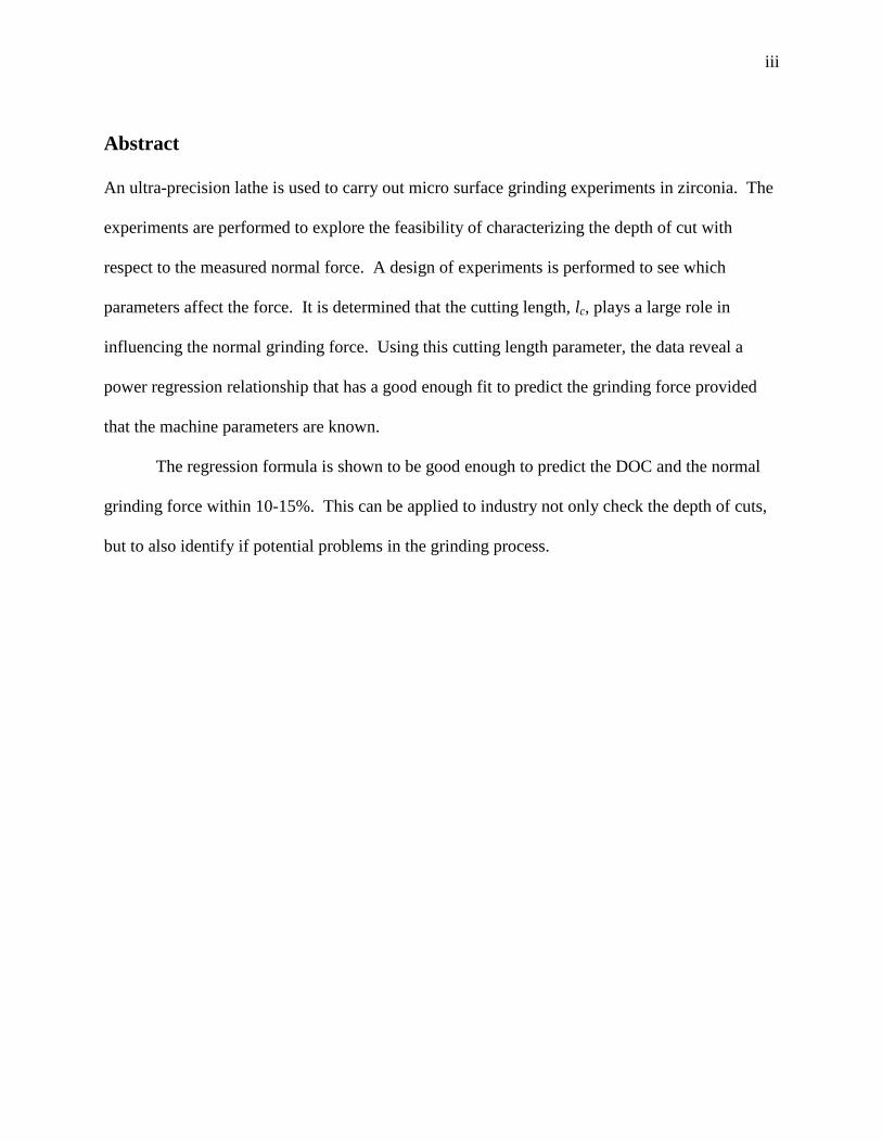
An ultra-precision lathe is used to carry out micro surface grinding experiments in zirconia. The
experiments are performed to explore the feasibility of characterizing the depth of cut with
respect to the measured normal force. A design of experiments is performed to see which
parameters affect the force. It is determined that the cutting length, lc, plays a large role in
influencing the normal grinding force. Using this cutting length parameter, the data reveal a
power regression relationship that has a good enough fit to predict the grinding force provided
that the machine parameters are known.
The regression formula is shown to be good enough to predict the DOC and the normal
grinding force within 10-15%. This can be applied to industry not only check the depth of cuts,
but to also identify if potential problems in the grinding process.
iv
Table of Contents
List of Figures ................................................................................................................................ vi
List of Tables ................................................................................................................................. ix
Acknowledgements ......................................................................................................................... x
Chapter 1 Introduction .................................................................................................................... 1
1.1 Background ........................................................................................................................... 1
1.2 Research Objective ................................................................................................................ 5
1.3 Literature Review .................................................................................................................. 6
1.3.1 Surface Grinding............................................................................................................. 7
1.3.2 Equivalent Chip Thickness ........................................................................................... 10
1.3.2 Similar Work in Zirconia .............................................................................................. 12
1.4 Approach ............................................................................................................................. 13
Chapter 2 Experimental Setup ...................................................................................................... 14
2.1 Machine and Setup .............................................................................................................. 14
2.2 Grinding Program ................................................................................................................ 19
2.3 Preparation of the Grinding Wheel ..................................................................................... 22
2.4 Preparation of the Zirconia Puck ......................................................................................... 23
Chapter 3 Experimental Procedure ............................................................................................... 26
3.1 Design of Experiments ........................................................................................................ 26
3.2 Accounting for Wheel Wear ............................................................................................... 27
3.3 Reducing Variability between Test Samples ...................................................................... 28
3.4 Verification of the Dynamometer ....................................................................................... 29
3.5 Data Post-Processing ........................................................................................................... 30
Chapter 4 Results .......................................................................................................................... 32
4.1 First Run: The Worn Wheel ................................................................................................ 32
v
4.1.1 Derivation of the Regression Model ............................................................................. 34
4.1.2 Sources of Error ............................................................................................................ 46
4.2 Second Run: Fresh Dressed Wheel ..................................................................................... 47
4.2.1 Sources of Error ............................................................................................................... 55
Chapter 5 Additional Observations ............................................................................................... 56
5.1 Comparison of the Two Wheels .......................................................................................... 56
5.2 Zero MRR Rubbing Forces at Depth .................................................................................. 57
5.3 Surface Finish ...................................................................................................................... 59
Chapter 6 Conclusion .................................................................................................................... 62
Appendix A: Machining Programs ............................................................................................... 64
A.1 DressWheel.NC .................................................................................................................. 64
A.2 FaceZirconia.NC ................................................................................................................ 66
A.3 FaceZirconiaVSandCSS.NC .............................................................................................. 67
A.4 GrindForceSamples.NC ..................................................................................................... 71
A.5 GrindPatches.NC ................................................................................................................ 78
Appendix B: Matlab Programs ..................................................................................................... 83
B.1 riptextdata.m ....................................................................................................................... 83
B.2 DataConditioningPlot.m ..................................................................................................... 84
B.3 CupGrindAnalysis.m .......................................................................................................... 85
B.4 PredictDOCusingh_eq.m .................................................................................................... 88
B.5 Predict DOCusingh_eqdst.m .............................................................................................. 90
B.6 Force Extraction Programs in report form.m...................................................................... 92
References ..................................................................................................................................... 95
vi
List of Figures
Figure 1.1 Effect of grinding forces on wheel deflection and real depth of cut. Source: Rowe,
2014 [1] ........................................................................................................................................... 3
Figure 1.2 Elements of a basic grinding system. Source: Rowe, 2014 [5] .................................... 7
Figure 1.3 Removal rate and specific removal rate for horizontal axis surface grinding. Source:
Rowe, 2014 [1]................................................................................................................................ 9
Figure 1.4 Definition of the equivalent grinding thickness heq in cylindrical (a) and in surface (b)
grinding. Source: Snoeys, 1984 [3]............................................................................................... 11
Figure 2.1 Chuck assembly with zirconia mounted on top of steel chuck. All dimensions in mm.
....................................................................................................................................................... 16
Figure 2.2 Large silicon carbide grinding wheel for truing the small diamond wheel. ............... 17
Figure 2.3 Setup for facing the zirconia sample to prepare experiments with the 50k spindle. .. 18
Figure 2.4 Solid model of grinding wheel relative to the zirconia chuck assembly .................... 20
Figure 2.5 Close up of grinding parameters. All values are in mm. ............................................ 21
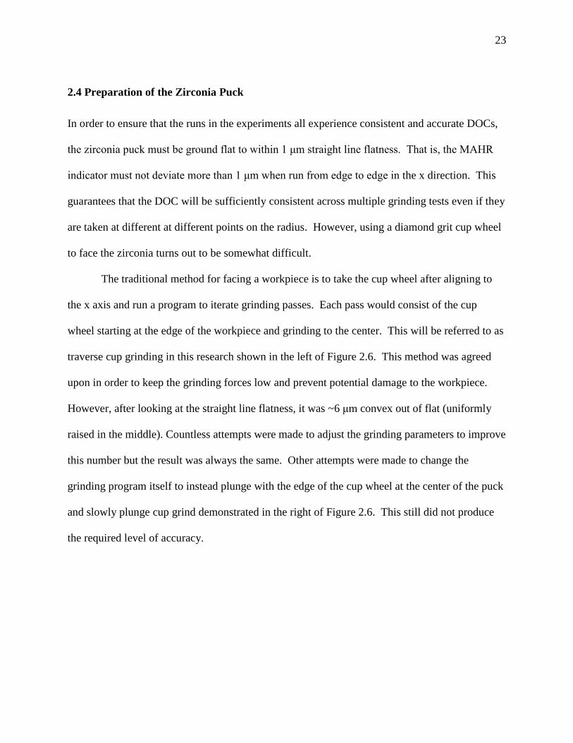
Figure 2.6 Zirconia cup grinding scenarios. [left] traverse and [right] plunge cup grinding ...... 24
Figure 2.7 Simulation of cup grinding conditions ....................................................................... 25
Figure 3.1 Verification test of the Kistler® dynamometer .......................................................... 29
Figure 3.2 Example of data conditioning for evaluation of grinding force. Filtering removes the
variation occurring at the rate of the grinding wheel rotation. ..................................................... 30
Figure 3.3 Close up of the filtering used to remove the grinding wheel influence ...................... 31
Figure 4.1 Adjusted normal force plot, the Fn is adjusted according to the heq for the worn wheel
....................................................................................................................................................... 32
vii
Figure 4.2 Grouped plot of the force per unit volume removed plotted over the MRR for the
worn wheel .................................................................................................................................... 33
Figure 4.3 Grinding variable main effects plot for MRR for the worn wheel ............................. 34
Figure 4.4 Grinding variable main effects plot for the normal force for the worn wheel ............ 35
Figure 4.5 Grinding variable main effects plot for the normal force per unit volume for the worn
wheel ............................................................................................................................................. 36
Figure 4.6 Grouped plot of the nN/um4
(force per unit volume per length of contact, lc) vs MRR
for the worn wheel ........................................................................................................................ 37
Figure 4.7 Grouped plot of nN/um4 (force per unit volume per length of contact, lc) vs heq for the
worn wheel .................................................................................................................................... 38
Figure 4.8 Grouped plot of nN/μm 4
vs heq/st (equivalent chip thickness per stepover) for the
worn wheel .................................................................................................................................... 39
Figure 4.9 Grinding variable main effects plot for the power regression model predicted forces
....................................................................................................................................................... 41
Figure 4.10 Grouped plot of the real normal force data vs MRR for the worn wheel ................. 42
Figure 4.11 Grouped plot of the predicted normal forces (F_p) vs MRR using the power
regression model from the worn wheel for DOC=25μm overlaid with the real force data .......... 43
Figure 4.12 Grouped plot of the predicted normal forces (F_p) vs MRR using the power
regression model from the worn wheel for DOC=35μm overlaid with the real force data .......... 44
Figure 4.13 Grouped plot of the predicted normal forces (F_p) vs MRR using the power
regression model from the worn wheel for DOC=45μm overlaid with the real force data .......... 45
Figure 4.14 Plot comparing the DOC predictions from both models for the worn wheel ........... 46
Figure 4.15 Grouped plot for µN/μm 3
vs MRR for the redressed wheel .................................... 47
viii
Figure 4.16 Grouped plot for nN/μm 4
(force per unit volume per length of contact, lc) vs heq for
the redressed wheel ....................................................................................................................... 48
Figure 4.17 Grouped plot for nN/μm 4
vs heq/st (equivalent chip thickness per stepover) for the
redressed wheel ............................................................................................................................. 49
Figure 4.18 Grouped plot of the real normal force data vs MRR for the redressed wheel .......... 51
Figure 4.19 Grouped plot of the predicted normal forces (F_p) vs MRR using the power
regression model from the redressed wheel for DOC=25μm overlaid with the real force data ... 52
Figure 4.20 Grouped plot of the predicted normal forces (F_p) vs MRR using the power
regression model from the redressed wheel for DOC=25μm overlaid with the real force data ... 53
Figure 4.21 Grouped plot of the predicted normal forces (F_p) vs MRR using the power
regression model from the redressed wheel for DOC=25μm overlaid with the real force data ... 54
Figure 4.22 Plot comparing the DOC predictions from both models for the redressed wheel .... 55
Figure 5.1 Plot comparing main effects trends for the force results of both wheels ................... 56
Figure 5.2 Grouped plot of normal force vs MRR with regression lines for the redressed wheel
....................................................................................................................................................... 57
Figure 5.3 Comparison of linear regression values for normal force for both wheels ................ 58
Figure 5.4 Zygo MetroSurf surface data output. Note that the 100 micrometer stepover is visible
in the surface profile as indicated by the darker grooves in green-blue. ...................................... 60
Figure 5.5 Microscope image a ground zirconia patch under 500x magnification. Grinding
passes run diagonally. The brittle mode is visible in the rough surface. ..................................... 61
ix
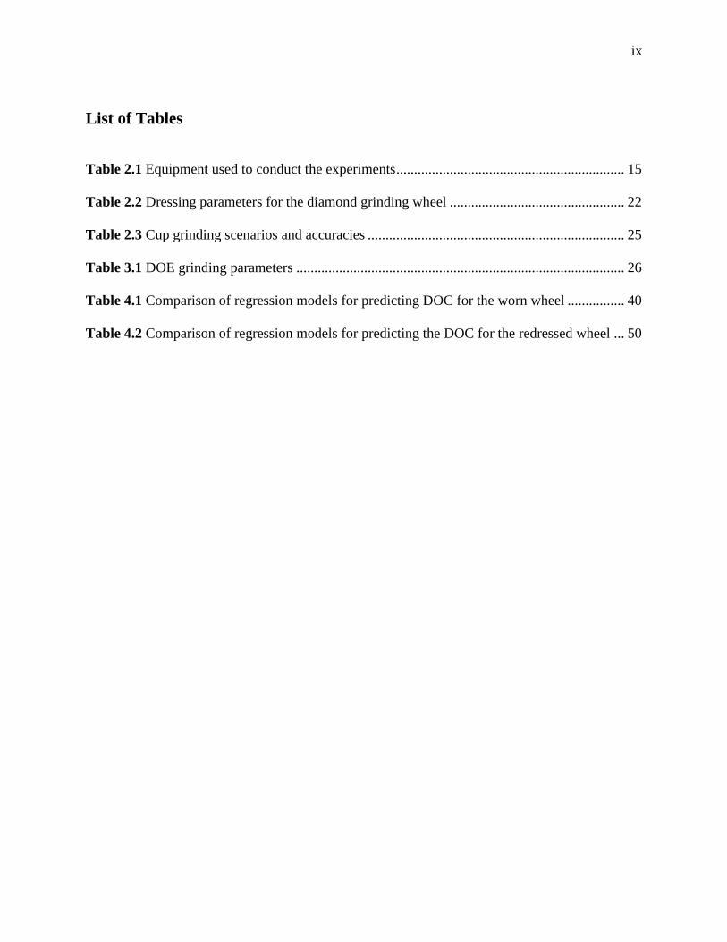
List of Tables
Table 2.1 Equipment used to conduct the experiments ................................................................ 15
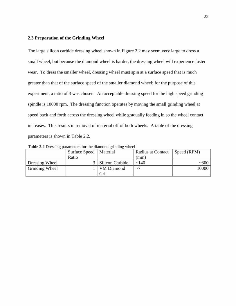
Table 2.2 Dressing parameters for the diamond grinding wheel ................................................. 22
Table 2.3 Cup grinding scenarios and accuracies ........................................................................ 25
Table 3.1 DOE grinding parameters ............................................................................................ 26
Table 4.1 Comparison of regression models for predicting DOC for the worn wheel ................ 40
Table 4.2 Comparison of regression models for predicting the DOC for the redressed wheel ... 50
x
Acknowledgements
The amazing opportunity to work in the Machine Dynamics Research Lab would not have been
possible without the gracious support of the John Bruning Fellowship and for which I am deeply
grateful. Dr. Bruning is a Penn State alumnus and incredibly accomplished engineer with notable
contributions to high accuracy interferometry and photolithography. His accomplishments served
as great inspiration and motivation during my time as a Master's student.
I would like to thank my advisor, Dr. Eric Marsh for his support, guidance and patience.
He showed me the importance of hard work and the resolve to figure out a problem on your own.
I owe much of the success of this project to Professional Instruments Company,
specifically David Arneson, for the research subject, samples and equipment. Their
contributions made this research possible.
I would also like to thank Dr. Eric Keller for his (reluctant) assistance in many aspects of
my research. His help was invaluable in setting up the equipment that made this research
possible. Working with both Dr. Eric Marsh and Dr. Eric Keller has definitely enriched my time
at Penn State and is experience I will not soon forget.
I would also like to thank my close friends that I have made during my time at the
Pennsylvania State University. I specifically want to thank Raveen Fernando and Kenneth
Swidwa. Their friendship and collaboration both on and off campus was crucial for me to have a
positive experience as a student new to the area. Finally, I want to thank my parents for their
never ending support and love.

1
Chapter 1 Introduction
1.1 Background
New materials are constantly being developed for demanding applications in current and
emerging high tech. These materials are engineered or selected for their properties to advance
the end product. This can present new challenges for the manufacture and machining of these
new materials.
Zirconium oxide, also known as zirconia, is a ceramic material with favorable properties
which include, hardness, high modulus of elasticity, low thermal conductivity and high wear
resistance. A key property that sets zirconia apart from other ceramic materials is the high
resistance to crack propagation. For these reasons it is desirable for use in demanding
applications, such as fixturing for precision application. It has also emerged in the medical field
for use in implants.
The properties that make zirconia a favorable material also make it difficult to machine.
This is also compounded with the fact that to be used in these demanding applications, precision
and surface finish are paramount. High volume machining processes such as milling are
unfeasible because the machine tools used will become damaged or excessively worn. They are
also unsuited to providing the required finished results, especially in ceramics. Ceramics, being
brittle materials, will become damaged when machined with large or dramatic forces. This
appears as subsurface damage and crack propagation, and is unacceptable in these advanced
applications.
2
Grinding is the best process to properly machine zirconia and is the practiced choice for
machining hard ceramics. Grinding results in relatively small grinding forces because, as
opposed to other cutting tools such as those used in milling, a grinding wheel employs many
small cutting edges instead of 1 or a few large cutting edges. Crack propagation as a result of
dramatic forces is mitigated in grinding, because of these small cutting edges. The subsurface
damage can also be better controlled by adjusting the parameters of the grind.
When grinding small features in zirconia (or any material that requires precise control of
the workpiece geometry), shaping or dressing the grinding wheel can take up a lot of time that
adds to the cost of manufacturing. The wheel must be properly measured and aligned to the
workpiece. If the wheel wears down faster than expected that can lead to scrapped parts and the
timely process of setting up the wheel again. Of equal importance is the confidence that the
machined features are the correct dimensions and quality. Zirconia is a hard material, so when
grinding, it is common that the programmed or intended depth of cut (DOC) may not match the
actual machined depth of cut. Usually the actual DOC is smaller than the programmed DOC
because of compliance in the machine tool. These factors are described in Rowe [1] as
“workpiece hardness, grinding wheel sharpness, machine tool stiffness, grinding wheel stiffness,
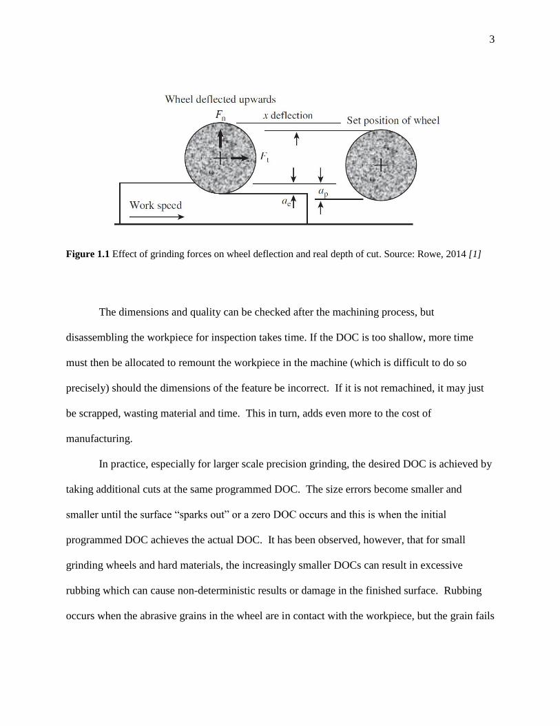
contact width, work speed and wheel speed.” This principle is demonstrated by Figure 1.1.
3
Figure 1.1 Effect of grinding forces on wheel deflection and real depth of cut. Source: Rowe, 2014 [1]
The dimensions and quality can be checked after the machining process, but
disassembling the workpiece for inspection takes time. If the DOC is too shallow, more time
must then be allocated to remount the workpiece in the machine (which is difficult to do so
precisely) should the dimensions of the feature be incorrect. If it is not remachined, it may just
be scrapped, wasting material and time. This in turn, adds even more to the cost of
manufacturing.
In practice, especially for larger scale precision grinding, the desired DOC is achieved by
taking additional cuts at the same programmed DOC. The size errors become smaller and
smaller until the surface “sparks out” or a zero DOC occurs and this is when the initial
programmed DOC achieves the actual DOC. It has been observed, however, that for small
grinding wheels and hard materials, the increasingly smaller DOCs can result in excessive
rubbing which can cause non-deterministic results or damage in the finished surface. Rubbing
occurs when the abrasive grains in the wheel are in contact with the workpiece, but the grain fails
4
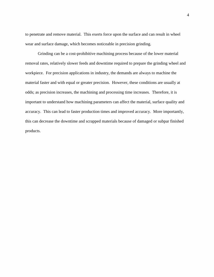
to penetrate and remove material. This exerts force upon the surface and can result in wheel
wear and surface damage, which becomes noticeable in precision grinding.
Grinding can be a cost-prohibitive machining process because of the lower material
removal rates, relatively slower feeds and downtime required to prepare the grinding wheel and
workpiece. For precision applications in industry, the demands are always to machine the
material faster and with equal or greater precision. However, these conditions are usually at
odds; as precision increases, the machining and processing time increases. Therefore, it is
important to understand how machining parameters can affect the material, surface quality and
accuracy. This can lead to faster production times and improved accuracy. More importantly,
this can decrease the downtime and scrapped materials because of damaged or subpar finished
products.
5
1.2 Research Objective
The objective of this research is to examine the feasibility of insitu monitoring of forces
experienced in grinding small features in Zirconia to determine the DOC. A secondary result of
this will be to analyze the effect of wheel wear on the grinding forces. These efforts will also
help to identify parameters for ideal grinding conditions.
Using a small radius grinding wheel, a large swath of parameters are analyzed in a
precision ground sample of Zirconia. The force is recorded using a dynamometer and then
analyzed with respect to the grinding conditions. The data taken will be used to determine
guidelines on selecting favorable grinding parameters as well as determining how the measured
forces are influenced by said grinding parameters. The culmination of this data is then used to
create an applicable model for predicting the DOC given a set of grinding parameters and the
measured force.

6
1.3 Literature Review
Grinding is an exhaustively studied process with years of literature detailing the science, in
addition to extensive catalogues of grinding data and guides. A great introductory resource to
grinding is provided in the Rowe, “Principles of Modern Grinding Technology Second Edition.”
[2] Throughout this paper, the principles established in Snoeys and Peters, “The Significance of
Chip Thickness in Grinding” [3] will also be utilized thoroughly.
This research emphasizes a grinding value called the equivalent chip thickness which
must be understood when analyzing grinding data. For that purpose, the equivalent chip
thickness is reviewed in detail. Finally, work of a similar nature submitted to the CIRP [4] is
also reviewed.

7
1.3.1 Surface Grinding
Ceramics usually require the use of grinding for machining. This is because zirconia is hard and
brittle and other machining process will likely lead in failure (damage to the tools and
workpiece). For hard ceramics like Zirconia, a diamond abrasive is required because, as a
general rule, the cutting material should be harder than the material removed. Zirconia is very
hard so the options are limited as the common grinding materials such as aluminum oxide and
silicon carbide have comparable hardnesses.
This research focuses on surface grinding albeit, on the micro scale. That is, the grinding
in this research is on the micron level with accuracies and surface roughnesses on the sub-micron
level. A general diagram of the basic surface grinding condition in this research is shown in
Figure 1.2, courtesy of Rowe [5].
Figure 1.2 Elements of a basic grinding system. Source: Rowe, 2014 [5]
8
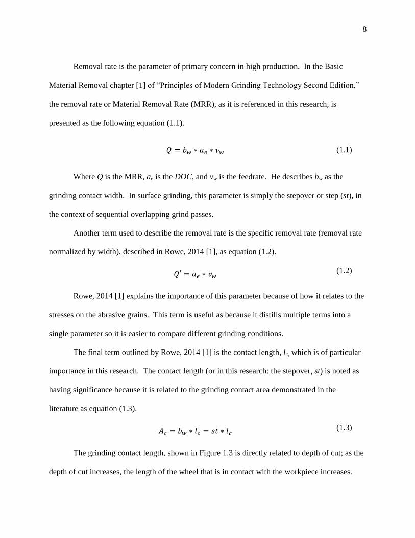
Removal rate is the parameter of primary concern in high production. In the Basic
Material Removal chapter [1] of “Principles of Modern Grinding Technology Second Edition,”
the removal rate or Material Removal Rate (MRR), as it is referenced in this research, is
presented as the following equation (1.1).
𝑄 = 𝑏𝑤 ∗ 𝑎𝑒 ∗ 𝑣𝑤 (1.1)
Where Q is the MRR, ae is the DOC, and vw is the feedrate. He describes bw as the
grinding contact width. In surface grinding, this parameter is simply the stepover or step (st), in
the context of sequential overlapping grind passes.
Another term used to describe the removal rate is the specific removal rate (removal rate
normalized by width), described in Rowe, 2014 [1], as equation (1.2).
𝑄′ = 𝑎𝑒 ∗ 𝑣𝑤 (1.2)
Rowe, 2014 [1] explains the importance of this parameter because of how it relates to the
stresses on the abrasive grains. This term is useful as because it distills multiple terms into a
single parameter so it is easier to compare different grinding conditions.
The final term outlined by Rowe, 2014 [1] is the contact length, lc, which is of particular
importance in this research. The contact length (or in this research: the stepover, st) is noted as
having significance because it is related to the grinding contact area demonstrated in the
literature as equation (1.3).
𝐴𝑐 = 𝑏𝑤 ∗ 𝑙𝑐 = 𝑠𝑡 ∗ 𝑙𝑐 (1.3)
The grinding contact length, shown in Figure 1.3 is directly related to depth of cut; as the
depth of cut increases, the length of the wheel that is in contact with the workpiece increases.
9
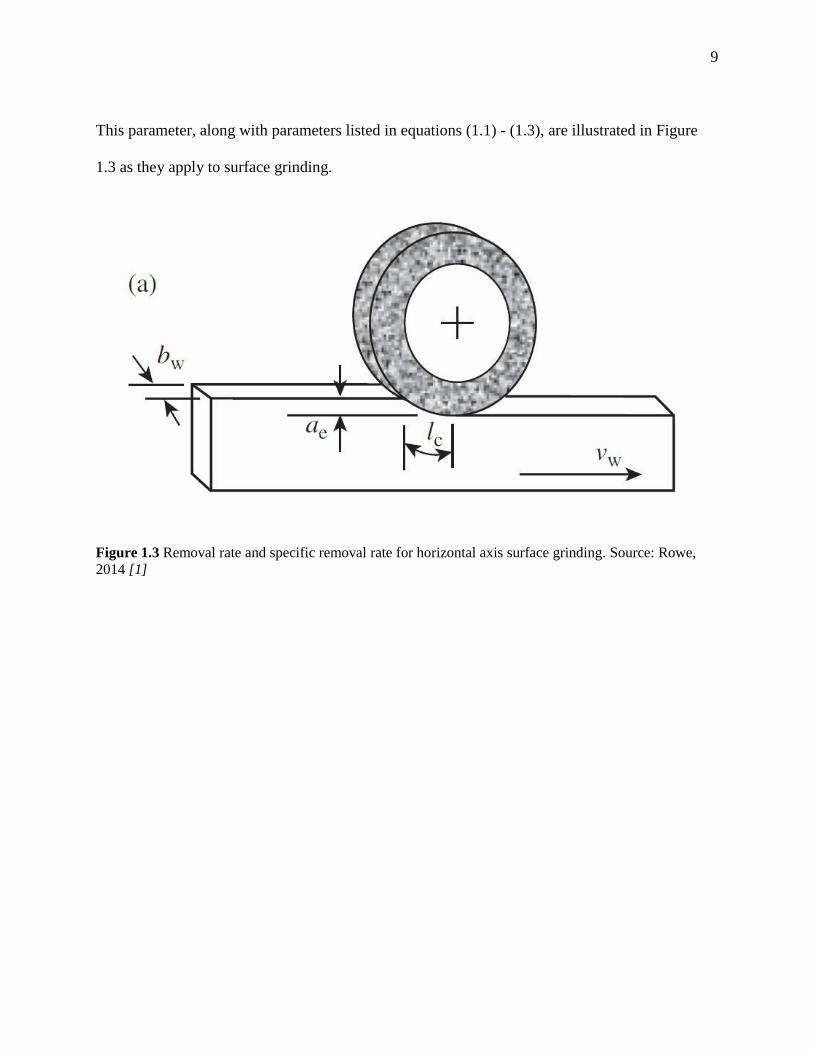
This parameter, along with parameters listed in equations (1.1) - (1.3), are illustrated in Figure
1.3 as they apply to surface grinding.
Figure 1.3 Removal rate and specific removal rate for horizontal axis surface grinding. Source: Rowe,
2014 [1]
10
1.3.2 Equivalent Chip Thickness
There is an abundance of literature and quantitative research on surface grinding. However,
much of the values observed can diverge based upon small changes to the grinding parameters.
In Snoeys and Peters, “The Significance of Chip Thickness in Grinding,” [3] they conclude that
there is a critical grinding value called the equivalent chip thickness, heq, shown in equation
(1.4).
ℎ𝑒𝑞 =𝑎
𝑞=
𝑎 ∗ 𝑣𝑤
𝑣𝑠=
𝐷𝑂𝐶 ∗ 𝑣𝑤
2𝜋 ∗ 𝑤ℎ𝑒𝑒𝑙𝑟𝑎𝑑𝑖𝑢𝑠 ∗ 𝑤ℎ𝑒𝑒𝑙𝑅𝑃𝑀
(1.4)
Where a is the DOC and q is the speed ratio of the surface speed of the grinding wheel,
vs, versus the surface speed, vw, (or feed rate) of the workpiece. The paper [3] describes the heq
to define the thickness the “continuous material layer” that is removed in a single grinding pass.
This is a result of the interaction of the competing surface speeds and the cutting depth of the
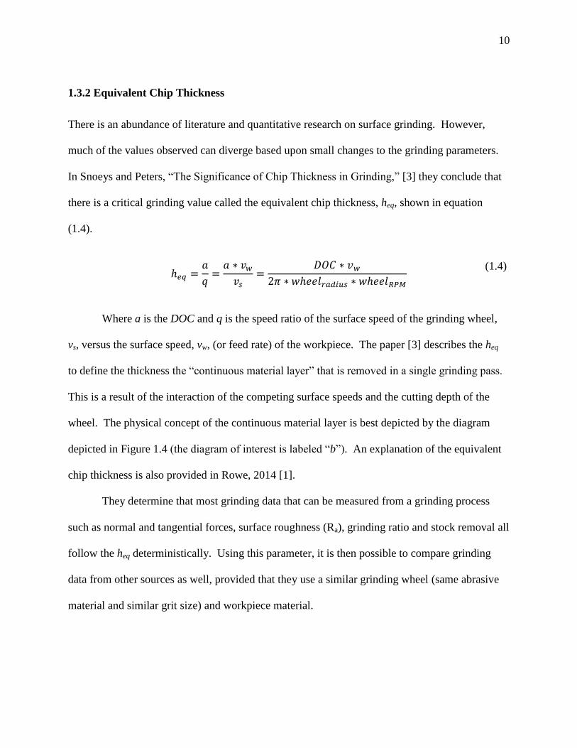
wheel. The physical concept of the continuous material layer is best depicted by the diagram
depicted in Figure 1.4 (the diagram of interest is labeled “b”). An explanation of the equivalent
chip thickness is also provided in Rowe, 2014 [1].
They determine that most grinding data that can be measured from a grinding process
such as normal and tangential forces, surface roughness (Ra), grinding ratio and stock removal all
follow the heq deterministically. Using this parameter, it is then possible to compare grinding
data from other sources as well, provided that they use a similar grinding wheel (same abrasive
material and similar grit size) and workpiece material.
11
Figure 1.4 Definition of the equivalent grinding thickness heq in cylindrical (a) and in surface (b)
grinding. Source: Snoeys, 1984 [3]
Snoeys and Peters [3] conclude that the forces measured in grinding follow a linear trend
when they’ve been normalized according to the heq, shown in equation (1.5).
𝐹𝑛′ =
𝐹𝑛
𝑤𝑤ℎ𝑒𝑒𝑙∗ ℎ𝑒𝑞 (1.5)
Where Fn is the normal force and wwheel is the width (or cutting edge length) of the wheel.
This linear trend is observed when the F’n is plotted versus the heq on a log-log plot. That is, the
data will follow a power regression trend.
12
1.3.2 Similar Work in Zirconia
A comparable study was performed in Zirconia by M. Rabiey, N. Jochum and F. Kuster [4]
titled, “High performance grinding of zirconium oxide (ZrO2) using hybrid bond diamond tools.”
The scope of their study covered a much wider range of grinding parameters. The range of
grinding parameters that they examined were also of much higher magnitudes (higher DOCs,
RPMs and feedrates), but their findings provide a great frame of reference for the work in this
research. The diamond grinding wheel used also had a much larger grain size, four to five times
larger than the grain size of the diamond wheel used in this research.
One particular point of interest is their examination of the brittle to ductile transition
range for zirconia. Their observation is that the transition zone, for their tests in Zirconia, is
when the uncut chip thickness, hcu, is ~1 micron (μm). The uncut chip thickness or the
maximum chip thickness is similar to the equivalent chip thickness and is also very similar in
value as well. The maximum chip thickness is very specific to certain grinding parameters as it
is applied, while the equivalent chip thickness is more versatile and can be better used to
facilitate in the comparison over a much wider set of grinding parameters.
Another take away from this literature is the lack of significant wheel wear that was
noticed despite having specific removal rate of 7800 mm3/mm. This is important because the
experiments conducted in this research have a maximum specific material removal of 0.0095
mm3/mm. Even if the specific removal rates were to be scaled based upon the grain size of the
applied wheels, the specific removal rate in the literature without observable wheel wear is still
orders of magnitude more than the specific removal rate used in this research.
13
1.4 Approach
Of the literature examined, there was no effort to characterize the DOC with respect to the
measured grinding force and applied grinding parameters. Therefore, this presents a unique
opportunity for this research to determine whether it is feasible. This research will analyze
forces for a range of parameters for the application of micro-grinding small features (such as
pockets) in zirconia. The zirconia will be precision mounted and aligned in an ultra-precision
lathe to simulate surface micro-grinding. The rotational axis of the work spindle will simulate
the horizontal axis, while a grinding wheel will be mounted on the z axis will simulate the
vertical axis. The zirconia will be affixed to a high resolution dynamometer and the in situ
normal grinding forces will be recorded at a high sampling rate. Only the normal grinding force
is analyzed because it is mounted on a rotary axis. An ultra-precision high speed spindle will
operate a trued-in-assembly small-radius diamond grinding wheel. Trued-in-assembly here
means that the grinding wheel is dressed/trued to the same axis as the face of the zirconia sample
while in the machine. Because this is a micro-grinding application, accuracies on the order of 1-
2 microns with sub-micron surface roughnesses will be targeted.
The forces, after recording, will be analyzed and conditioned based upon the applicable
grinding parameters to observe and establish trends that can be used to characterize the DOC.
The end result being that with the known parameters of the surface grind, the stepover (or
according to Rowe, 2014 [1], the grinding contact width, bw) and the feedrate, vw, and the
measured force, the DOC can be determined within a reasonable margin of error. The additional
observations derived from the grinding data will be used to determine guidelines on selecting
optimal grinding parameters as well as directions for further work in this research.

14
Chapter 2 Experimental Setup
2.1 Machine and Setup
The machine used for this research is a Moore Nanotech Ultra-Precision Lathe (UPL) 450.
Being a lathe (which operates horizontally), the grinding experiments are conducted horizontally.
The work spindle is used for the horizontal axes. The UPL is fitted with a Professional
Instruments 50K ISO high-speed ultra-precision airbearing spindle equipped with a small,
diamond grit wheel.
As part of the complete setup, the machine is fitted with another motorized Professional
Instruments 4R airbearing spindle with a diamond cup wheel. These tests require the utmost
precision; both tool spindles must be utilized in conjunction without any disassembly between
steps. On the work spindle of the machine, a Kistler® Dynamometer is fitted. This is where the
zirconia will be mounted and is how the grinding force data will be collected. All materials are
listed in Table 2.1 with all of the applicable equipment used in the setup and execution of the
grinding experiments.
15
Table 2.1 Equipment used to conduct the experiments Equipment Designation Manufacturer Description/Purpose
Machine Nanotech UPL (Ultra-Precision
Lathe) 450
Moore Nanotech Ultra-Precision Lathe used for
extremely demanding precision
applications in industry and academia.
Chiller ThermoFlex 1400 Thermo Fischer
Scientific
Used to maintain the operating
temperature of the 50k airbearing
spindle.
Indicator Ultra-Precision Ruby-tipped
LVDT Lever head indicator
Mahr (distributed
by Moore
Nanotech)
Used to measure, align and check
components in assembly within the
machine.
3 Axis Dynamometer Kistler® MiniDyn Type 9256A2 KISTLER Used to measure the normal grinding
force
DAQ (data
acquisition unit and
software)
Abaqus 901 Vibration Controller Data Physics
Corporation
Used to collect data at a sufficiently
high Hz above the frequency of the
grinding spindle. Employs anti-aliasing
filters for improved confidence.
DataPhysics Suite Data Physics
Corporation
Stores and organizes collected data for
analysis.
Optical Inspection
Hardware
Zygo MetroSurf Microscope and
software
Zygo Uses light interference waves to
generate a surface model to analyze the
surface accuracy and roughness.
Oscilloscope Techtronic Used in conjunction with the
dynamometer to dynamically “touch
off” the grinding wheel to the
workpiece.
Data Post-Processing
Software
Matlab Mathworks Computational language and interface.
Spindles 5.5 ISO Bronze Bore Ultra-
Precision Airbearing
Professional
Instruments Co.
Work-spindle: holds the measuring
equipment and the workpiece (Zirconia
puck).
2.5 ISO 50k Ultra-Precision
Airbearing
Professional
Instruments Co.
Grinding spindle: operates the grinding
wheel for use in grinding the samples.
Motorized 4R BlockHead® Ultra-
Precision Airbearing
Professional
Instruments Co.
Operates the cup-grinding wheel used to
face/align the zirconia puck to the axis
of the machine
Grinding Wheels 1x1 cm 320 Vitreous Metal (VM)
Bonded Diamond Grit Wheel
Diagrind Inc. Diamond grit abrasive wheel. Precision
wheel mount graciously donated by
Professional Instruments Co.
Precision Diamond Grit Cup
Wheel
Professional
Instruments Co.
Used to true/align the zirconia puck to
the machine axis and the 50k spindle
wheel
Workpiece Zirconium Oxide Puck Professional
Instruments Co.
(Donated)
Sample grinding material
Chuck Adhesive JB Quick-Weld Epoxy JB Very stiff and strong epoxy used to
firmly affix the zirconia puck to the
chuck
Chuck Stainless Mild Steel Professional
Instruments Co.
This is machined with a special “glue
pocket” to accommodate the extra
volume required by the glue so the
workpiece can have intimate contact
with the puck and still be firmly
attached.
Coolant EcoCool 711 Fuchs Lubricates and carries away heat and
swarf away from the workpiece and
grinding wheel

16
The Zirconia is mounted on a mild stainless steel chuck with four counter-bored holes to
mate to the dynamometer. The chuck is ground flat to less than 1 μm on the surface, which has
also been ground flat to ensure stable contact. Then the chuck is turned using a CBN lathe tool
to feature a “glue pocket”, shown in the cross-section in Figure 2.1. This is a mid-radial space to
provide a pocket for epoxy with which to rigidly mount the zirconia to the steel puck. Toward
the outside edge of the channel, the pocket is deeper to catch spare epoxy as it is squeezed while
fixing the zirconia to the steel puck. This way the zirconia puck is supported in the center and
outer edge faces. The glue pocket is thin, ~0.2 μm, (it is larger in the diagram for visibility) so
the bond layer is stiff and in intimate contact with the two parts.
Figure 2.1 Chuck assembly with zirconia mounted on top of steel chuck. All dimensions in mm.
The grinding wheel and the zirconia are both trued in assembly to eliminate any possible
alignment errors. The grinding wheel must be absolutely parallel to the zirconia surface to
Very shallow
mid-radial pocket
Flange with counter-bored
holes to mount to the
dynamometer
Flat intimate contact with
the two ground flat surfaces
on the center and edge of
the puck
Deeper pocket towards the
edge to catch excess epoxy
17
conduct the grinding tests. A large silicon carbide wheel, demonstrated in Figure 2.2, dresses the
wheel and the grinding edge is evaluated visually. Because the wheel is mounted at a 45 angle,
truing the face of the wheel along the z-axis will simultaneously true the face parallel to the x
axis. In Figure 2.2, the dressing action happens on the outside diameter of the silicon carbide
wheel.
Figure 2.2 Large silicon carbide grinding wheel for truing the small diamond wheel.
Once the grinding wheel is trued, the silicon carbide wheel is removed and replaced with
the zirconia puck and the precision diamond cup wheel is mounted to the motorized 4R
BlockHead® spindle. The zirconia is ground flat and perpendicular to < 1 μm using the cup
Silicon carbide
dressing wheel
ISO 50K high speed
ultra-precision
airbearing spindle 320 VM bonded
diamond grit wheel
ISO 5.5 ultra-
precision airbearing
spindle
Coolant delivery system
18
wheel mounted on a motorized 4R, shown in the setup in Figure 2.3. To achieve this, both
grinding spindles are simultaneously mounted upon the z-axis table as demonstrated in the
following figures. After a complete set of grinding cycles have been executed and the zirconia
has been removed and the ground patches inspected, the zirconia and grinding wheel must be re-
trued. The zirconia assembly is fixed to a Kistler Dynamometer to measure the in-situ grinding
force, as shown in Figure 2.3.
Figure 2.3 Setup for facing the zirconia sample to prepare experiments with the 50k spindle.
It should be stated that all components and mounting plate fixtures have been ground flat
and parallel to around 1 nanometer or less, so when they are mounted to the spindles there is stiff
and stable contact between the surfaces. When the wheels are mounted they are “dialed in” or
adjusted so they are concentric to the rotating axis of the spindle to within 1 μm TIR (the parts
are indicated using the MAHR precision LVDT lever-head indicator).
Motorized 4R
BlockHead® ultra-
precision airbearing Coolant delivery system
Dynamometer: Kistler®
MiniDyn type 9256A2
Chuck assembly
with zirconia
puck
Precision diamond grit
cup wheel
Spacer to provide
clearance for the dressed
small diamond wheel
320 VM bonded
diamond grit
wheel: trued to
both the Z
and X
axis

19
2.2 Grinding Program
Because the machine is configured in a XZC arrangement, it cannot grind vertically as shown by
the surface grinding figures shown in the literature review. To conduct these experiments, the
grinding wheel (mounted horizontally) will grind in the tangent direction to the center of the
zirconia workpiece. To replicate the horizontal movement, the zirconia will rotate at an angular
velocity such that at the grinding contact somewhere on the radius, the surface speed of the
zirconia will be equivalent to the proposed feedrate parameters for the surface grind tests. The
grinding samples are small so the deviation from the straight direction will be negligible. Of
note is the length of the grinding force samples which are at the most ~200 μm. The grinding
samples will be taken near the edge of the zirconia sample which is ~20 mm. The radius is
roughly 2 orders of magnitude more than the maximum arc length of the grinding force samples.
For this reason, because of the short grinding distance, the travel can be considered as straight
without any meaning error due to the curved travel of the wheel as it traverses across the
zirconia. For visualization a solid model is shown in Figure 2.4 of the grinding wheel on the
zirconia workpiece.
20
Figure 2.4 Solid model of grinding wheel relative to the zirconia chuck assembly
It is important to keep in mind that to imitate normal grinding conditions, distance
between passes must be less than the trued grinding edge. The program is designed to start at the
outer edge of the workpiece and grind an initial pass at the programmed DOC. This initial pass
is crucial as it eliminates the full wheel edge length as a variable in the grinds (for multiple wheel
dressings). In these tests, the program is designed to very carefully control the grinding contact
width, or the stepover. The next pass, the grinding wheel will stepover toward the radius and this
pass will be measured for force feedback and the material removed will correspond precisely to
the programmed stepover. This process is shown in close up in Figure 1.1.
Stepover (st) direction
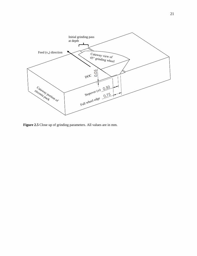
21
Figure 2.5 Close up of grinding parameters. All values are in mm.
Initial grinding pass
at depth
Feed (vw) direction
22
2.3 Preparation of the Grinding Wheel
The large silicon carbide dressing wheel shown in Figure 2.2 may seem very large to dress a
small wheel, but because the diamond wheel is harder, the dressing wheel will experience faster
wear. To dress the smaller wheel, dressing wheel must spin at a surface speed that is much
greater than that of the surface speed of the smaller diamond wheel; for the purpose of this
experiment, a ratio of 3 was chosen. An acceptable dressing speed for the high speed grinding
spindle is 10000 rpm. The dressing function operates by moving the small grinding wheel at
speed back and forth across the dressing wheel while gradually feeding in so the wheel contact
increases. This results in removal of material off of both wheels. A table of the dressing
parameters is shown in Table 2.2.
Table 2.2 Dressing parameters for the diamond grinding wheel
Surface Speed
Ratio
Material Radius at Contact
(mm)
Speed (RPM)
Dressing Wheel 3 Silicon Carbide ~140 ~300
Grinding Wheel 1 VM Diamond
Grit
~7 10000
23
2.4 Preparation of the Zirconia Puck
In order to ensure that the runs in the experiments all experience consistent and accurate DOCs,
the zirconia puck must be ground flat to within 1 μm straight line flatness. That is, the MAHR
indicator must not deviate more than 1 μm when run from edge to edge in the x direction. This
guarantees that the DOC will be sufficiently consistent across multiple grinding tests even if they
are taken at different at different points on the radius. However, using a diamond grit cup wheel
to face the zirconia turns out to be somewhat difficult.
The traditional method for facing a workpiece is to take the cup wheel after aligning to
the x axis and run a program to iterate grinding passes. Each pass would consist of the cup
wheel starting at the edge of the workpiece and grinding to the center. This will be referred to as
traverse cup grinding in this research shown in the left of Figure 2.6. This method was agreed
upon in order to keep the grinding forces low and prevent potential damage to the workpiece.
However, after looking at the straight line flatness, it was ~6 μm convex out of flat (uniformly
raised in the middle). Countless attempts were made to adjust the grinding parameters to improve
this number but the result was always the same. Other attempts were made to change the
grinding program itself to instead plunge with the edge of the cup wheel at the center of the puck
and slowly plunge cup grind demonstrated in the right of Figure 2.6. This still did not produce
the required level of accuracy.
24
Figure 2.6 Zirconia cup grinding scenarios. [left] traverse and [right] plunge cup grinding
The solution to get an accurate surface is more complicated than changing just the
grinding parameters. Through grinding tests, the convexity is revealed to be related to the length
of contact of each radial point on the zirconia puck. In short, because the outer parts of the
zirconia move faster than the center of the puck, more material is removed on those areas, hence
the convex shape. While this condition manifests in different ways for both cup grinding
scenarios, the end result is the same, an unacceptable convex shape.
The solution to this problem involves modifying the traverse cup grinding by first tilting
the cup grind spindle so that instead of grinding with the complete arc length that overlaps the
zirconia, the wheel only grinds with the leading edge and thus lowers the grinding force (this
helps the programmed DOC become closer the actual DOC). Then the traverse speed is adjusted
so the wheel starts out fast at the edge of the puck then slows down as it approaches the center,
this will be called variable feed. The final adjustment increases the rpm as the cup wheel
approached the center. This is called constant surface speed, but will here be referred to as
variable RPM. The result on the length of contact as the wheel approaches the center of the puck
is shown in Figure 2.7. The effects of each grinding scenario and their corresponding straight
line flatness is shown in Figure 2.7.
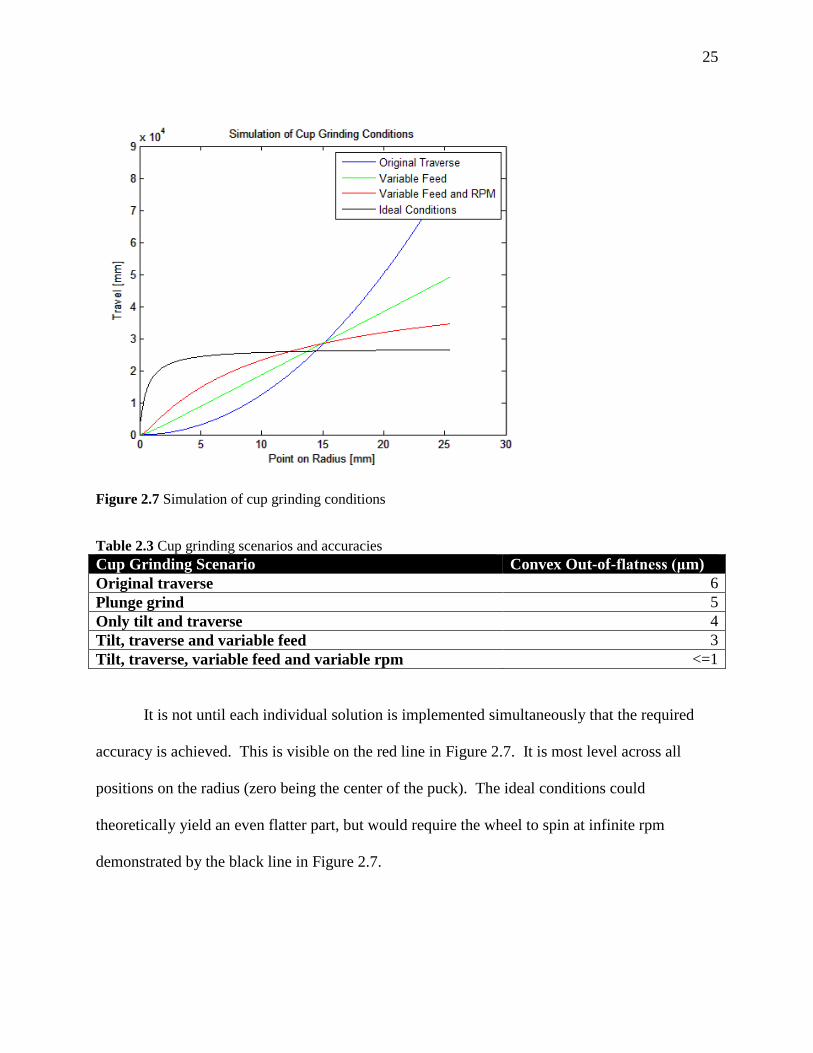
25
Figure 2.7 Simulation of cup grinding conditions
Table 2.3 Cup grinding scenarios and accuracies
Cup Grinding Scenario Convex Out-of-flatness (μm)
Original traverse 6
Plunge grind 5
Only tilt and traverse 4
Tilt, traverse and variable feed 3
Tilt, traverse, variable feed and variable rpm <=1
It is not until each individual solution is implemented simultaneously that the required
accuracy is achieved. This is visible on the red line in Figure 2.7. It is most level across all
positions on the radius (zero being the center of the puck). The ideal conditions could
theoretically yield an even flatter part, but would require the wheel to spin at infinite rpm
demonstrated by the black line in Figure 2.7.

26
Chapter 3 Experimental Procedure
3.1 Design of Experiments
The research proceeds with a standard factorial Design of Experiments (DOE). The variables
that are taken into account are the stepover (st), the feedrate (vw) and the DOC. The values of the
variables are shown in Table 3.1. These parameters were chosen because the feedrates were
small enough to be considered orders of magnitude smaller than the radius of the zirconia disk.
These parameters were also selected because they produce forces that are significant compared
to the cyclical forces of as the wheel is in contact with the Zirconia. Each sample is ground for 1
second 5 times. The short sample length is necessary to eliminate the dynamometer drift from
the sample force and is sufficient to reach a steady grinding state.
Table 3.1 DOE grinding parameters
DOC [μm] 25, 35, 45
Stepover (st) [μm] 100, 125, 150
Feedrate (vw) [μm/s] 60, 90 120, 150, 180, 210
27
3.2 Accounting for Wheel Wear
In reviewing the literature, past researchers conducting similar work in zirconia [4] observed
negligible wear despite having relatively high specific removal rates. It is mentioned that the
highest specific removal rate experienced by these grinding parameters is several orders of
magnitude smaller, while also using a diamond wheel. The largest equivalent chip thickness, heq,
in this set of parameters is 0.0043 μm, where the grain size of the wheel used is ~50 μm. Rowe,
2014 [6], also explains that there is a high correlation between the speed ratio and wheel wear
and that by having a high speed ratio, q, the equivalent chip thickness can be decreased enough
to greatly mitigate wheel wear. In dozens of test cuts before the experiments took place, the
measured forces were objectively the same. Therefore it can be reasonably concluded that in the
scope of a single run of tests, the wheel wear is negligible and the effect on the measured force is
very small compared to the resultant forces.
28
3.3 Reducing Variability between Test Samples
Besides recording the force during grinding, the dynamometer also serves another important
function in this research. When used with a standard oscilloscope, it is used to accurately
determine the “touch-off” location of the wheel the instant it comes into initial contact with the
workpiece. This diminishes the uncertainty in the DOC, which is critical for the reliability of the
experiments. Touching off with the dynamometer before and after each run of samples ensures
that there is no drift between batches. After many test cuts, the method of touching off while
actively monitoring the state of the dynamometer is proven to be well within 1 micron after
several test cuts are made to the experimental depth of cuts.
The Machine Dynamics Research Lab space can be prone to large (3° Celsius)
temperature swings during the day or when the weather changes drastically. Therefore, most of
these tests are conducted at night, except for the first run of tests (which also used a relatively
worn wheel for comparison purposes). This ensures that the machine sees the minimal thermal
drift during the individual grinding test cycles.
29
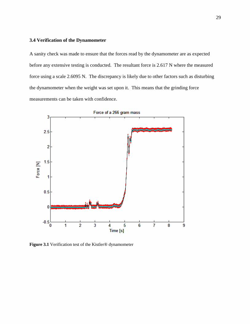
3.4 Verification of the Dynamometer
A sanity check was made to ensure that the forces read by the dynamometer are as expected
before any extensive testing is conducted. The resultant force is 2.617 N where the measured
force using a scale 2.6095 N. The discrepancy is likely due to other factors such as disturbing
the dynamometer when the weight was set upon it. This means that the grinding force
measurements can be taken with confidence.
Figure 3.1 Verification test of the Kistler® dynamometer

30
3.5 Data Post-Processing
Sensitive data collection of this nature can be subject to varying in ambient temperature or other
unforeseen conditions while collecting. Therefore the data is collected at the highest possible
collection rate and post processing of the collected data is required. The data is loaded and based
upon specific marks or triggers, the data is aligned precisely. From here the data can then be
evaluated all at once by executing a loop. Here all the data is cropped, filtered and the linear
deviations from drift and temperature are corrected. An example of the data before and after
conditioning is shown in Figure 3.2.
Figure 3.2 Example of data conditioning for evaluation of grinding force. Filtering removes the variation
occurring at the rate of the grinding wheel rotation.

31
The black line in the figure is the resultant grinding force of the grind. The machine is
programmed to take a precise cut at the programmed DOC and cut at the required feedrate using
the desired grinding contact width or stepover. Values are then taken off the observed plateau in
the black line and averaged to determine the real grinding force for that grind. This is one of
several samples collected using the exact same grinding parameters. Each of the many 1 second
samples is analyzed the same way, and then the average of all the plateau averages is returned as
the normal grinding force for that set of parameters. The large amplitude high frequency activity
in the original signal is a result of the dynamometer reacting to the once-per-revolution impulses
of the grinding wheel while in contact. This variation is well above the usable bandwidth of the
dynamometer and must be filtered out with a low-pass filter. The high frequency signal is also at
precisely the rpm of the grinding spindle (30,000 rpm) and is demonstrated in the high frequency
close up of the signal in Figure 3.3. Finally, the signal is cleaned up with a light rolling average
to get a crisp force profile for the grind. It can be seen precisely when the grinding wheel
contacts the zirconia puck and reaches steady state grinding before it stops and then retracts.
Figure 3.3 Close up of the filtering used to remove the grinding wheel influence
32
Chapter 4 Results
4.1 First Run: The Worn Wheel
While it was previously stated that within a single run of grinding tests, the wheel wear is
insignificant, the wheel used for this particular tests had already been subjected to the equivalent
wear of several full test runs. This provides the perfect opportunity to examine the forces of a
wheel that had relatively significant wear with a wheel that had been freshly dressed.
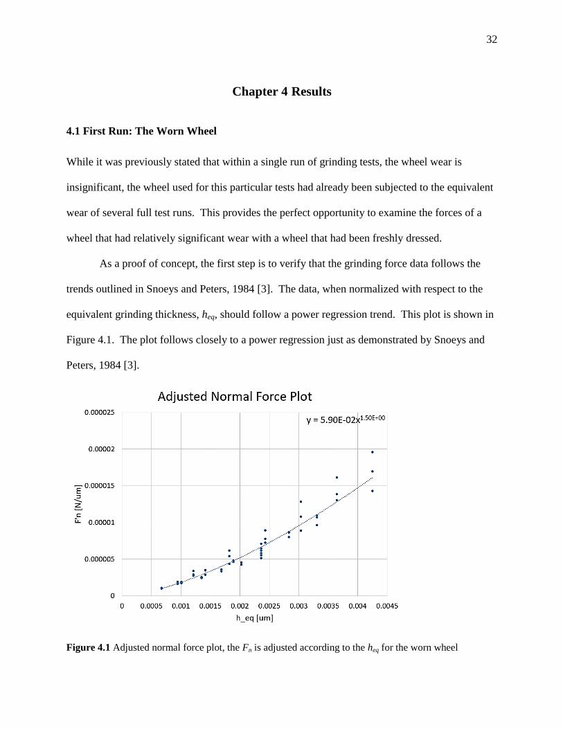
As a proof of concept, the first step is to verify that the grinding force data follows the
trends outlined in Snoeys and Peters, 1984 [3]. The data, when normalized with respect to the
equivalent grinding thickness, heq, should follow a power regression trend. This plot is shown in
Figure 4.1. The plot follows closely to a power regression just as demonstrated by Snoeys and
Peters, 1984 [3].
Figure 4.1 Adjusted normal force plot, the Fn is adjusted according to the heq for the worn wheel
33
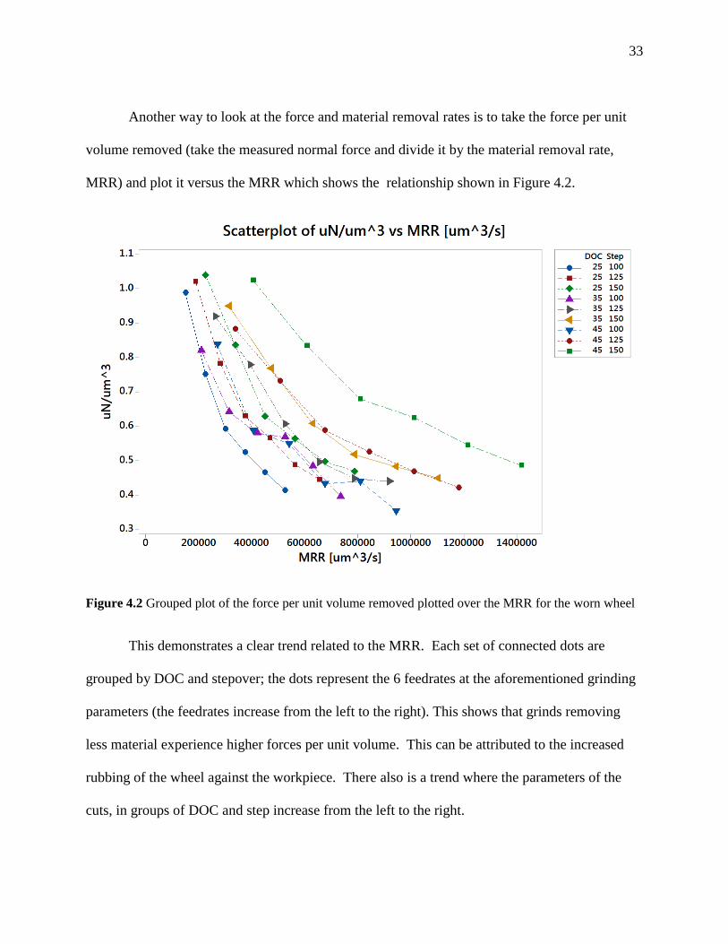
Another way to look at the force and material removal rates is to take the force per unit
volume removed (take the measured normal force and divide it by the material removal rate,
MRR) and plot it versus the MRR which shows the relationship shown in Figure 4.2.
Figure 4.2 Grouped plot of the force per unit volume removed plotted over the MRR for the worn wheel
This demonstrates a clear trend related to the MRR. Each set of connected dots are
grouped by DOC and stepover; the dots represent the 6 feedrates at the aforementioned grinding
parameters (the feedrates increase from the left to the right). This shows that grinds removing
less material experience higher forces per unit volume. This can be attributed to the increased
rubbing of the wheel against the workpiece. There also is a trend where the parameters of the
cuts, in groups of DOC and step increase from the left to the right.
34
4.1.1 Derivation of the Regression Model
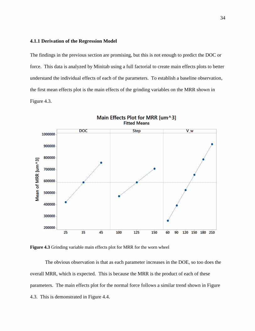
The findings in the previous section are promising, but this is not enough to predict the DOC or
force. This data is analyzed by Minitab using a full factorial to create main effects plots to better
understand the individual effects of each of the parameters. To establish a baseline observation,
the first mean effects plot is the main effects of the grinding variables on the MRR shown in
Figure 4.3.
Figure 4.3 Grinding variable main effects plot for MRR for the worn wheel
The obvious observation is that as each parameter increases in the DOE, so too does the
overall MRR, which is expected. This is because the MRR is the product of each of these
parameters. The main effects plot for the normal force follows a similar trend shown in Figure
4.3. This is demonstrated in Figure 4.4.
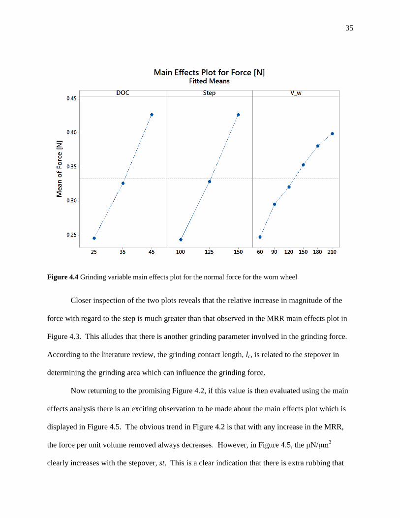
35
Figure 4.4 Grinding variable main effects plot for the normal force for the worn wheel
Closer inspection of the two plots reveals that the relative increase in magnitude of the
force with regard to the step is much greater than that observed in the MRR main effects plot in
Figure 4.3. This alludes that there is another grinding parameter involved in the grinding force.
According to the literature review, the grinding contact length, lc, is related to the stepover in
determining the grinding area which can influence the grinding force.
Now returning to the promising Figure 4.2, if this value is then evaluated using the main
effects analysis there is an exciting observation to be made about the main effects plot which is
displayed in Figure 4.5. The obvious trend in Figure 4.2 is that with any increase in the MRR,
the force per unit volume removed always decreases. However, in Figure 4.5, the μN/μm3
clearly increases with the stepover, st. This is a clear indication that there is extra rubbing that
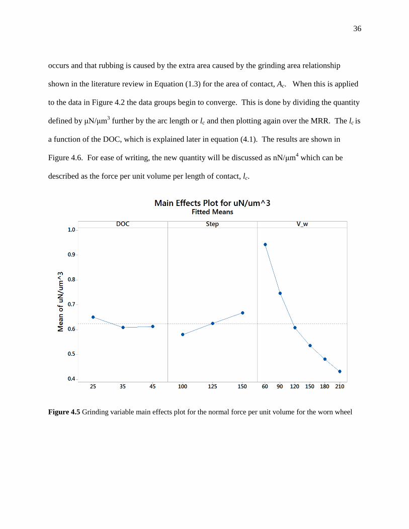
36
occurs and that rubbing is caused by the extra area caused by the grinding area relationship
shown in the literature review in Equation (1.3) for the area of contact, Ac. When this is applied
to the data in Figure 4.2 the data groups begin to converge. This is done by dividing the quantity
defined by μN/μm3 further by the arc length or lc and then plotting again over the MRR. The lc is
a function of the DOC, which is explained later in equation (4.1). The results are shown in
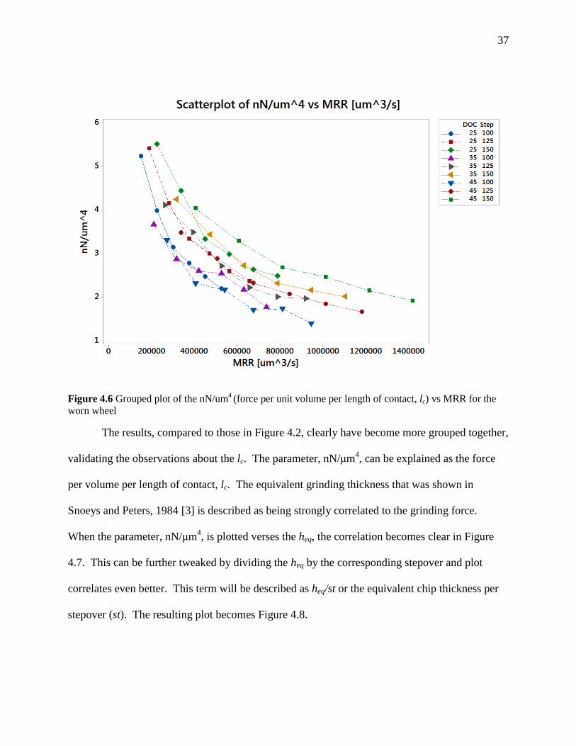
Figure 4.6. For ease of writing, the new quantity will be discussed as nN/μm4 which can be
described as the force per unit volume per length of contact, lc.
Figure 4.5 Grinding variable main effects plot for the normal force per unit volume for the worn wheel
37
Figure 4.6 Grouped plot of the nN/um4 (force per unit volume per length of contact, lc) vs MRR for the
worn wheel
The results, compared to those in Figure 4.2, clearly have become more grouped together,
validating the observations about the lc. The parameter, nN/μm4, can be explained as the force
per volume per length of contact, lc. The equivalent grinding thickness that was shown in
Snoeys and Peters, 1984 [3] is described as being strongly correlated to the grinding force.
When the parameter, nN/μm4, is plotted verses the heq, the correlation becomes clear in Figure
4.7. This can be further tweaked by dividing the heq by the corresponding stepover and plot
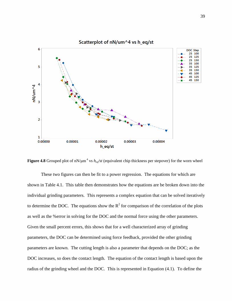
correlates even better. This term will be described as heq/st or the equivalent chip thickness per
stepover (st). The resulting plot becomes Figure 4.8.

38
Figure 4.7 Grouped plot of nN/um4 (force per unit volume per length of contact, lc) vs heq for the worn
wheel
39
Figure 4.8 Grouped plot of nN/μm 4 vs heq/st (equivalent chip thickness per stepover) for the worn wheel
These two figures can then be fit to a power regression. The equations for which are
shown in Table 4.1. This table then demonstrates how the equations are be broken down into the
individual grinding parameters. This represents a complex equation that can be solved iteratively
to determine the DOC. The equations show the R2 for comparison of the correlation of the plots
as well as the %error in solving for the DOC and the normal force using the other parameters.
Given the small percent errors, this shows that for a well characterized array of grinding
parameters, the DOC can be determined using force feedback, provided the other grinding
parameters are known. The cutting length is also a parameter that depends on the DOC; as the
DOC increases, so does the contact length. The equation of the contact length is based upon the
radius of the grinding wheel and the DOC. This is represented in Equation (4.1). To define the
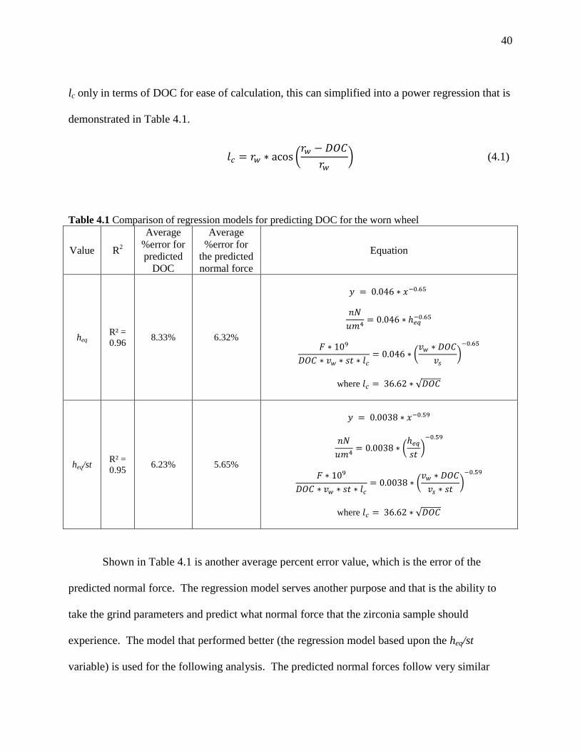
40
lc only in terms of DOC for ease of calculation, this can simplified into a power regression that is
demonstrated in Table 4.1.
𝑙𝑐 = 𝑟𝑤 ∗ acos (𝑟𝑤 − 𝐷𝑂𝐶
𝑟𝑤) (4.1)
Table 4.1 Comparison of regression models for predicting DOC for the worn wheel
Value R2
Average
%error for
predicted
DOC
Average
%error for
the predicted
normal force
Equation
heq R² =
0.96 8.33% 6.32%
𝑦 = 0.046 ∗ 𝑥−0.65
𝑛𝑁
𝑢𝑚4= 0.046 ∗ ℎ𝑒𝑞
−0.65
𝐹 ∗ 109
𝐷𝑂𝐶 ∗ 𝑣𝑤 ∗ 𝑠𝑡 ∗ 𝑙𝑐
= 0.046 ∗ (𝑣𝑤 ∗ 𝐷𝑂𝐶
𝑣𝑠
)−0.65
where 𝑙𝑐 = 36.62 ∗ √𝐷𝑂𝐶
heq/st R² =
0.95 6.23% 5.65%
𝑦 = 0.0038 ∗ 𝑥−0.59
𝑛𝑁
𝑢𝑚4= 0.0038 ∗ (
ℎ𝑒𝑞
𝑠𝑡)
−0.59
𝐹 ∗ 109
𝐷𝑂𝐶 ∗ 𝑣𝑤 ∗ 𝑠𝑡 ∗ 𝑙𝑐
= 0.0038 ∗ (𝑣𝑤 ∗ 𝐷𝑂𝐶
𝑣𝑠 ∗ 𝑠𝑡)
−0.59
where 𝑙𝑐 = 36.62 ∗ √𝐷𝑂𝐶
Shown in Table 4.1 is another average percent error value, which is the error of the
predicted normal force. The regression model serves another purpose and that is the ability to
take the grind parameters and predict what normal force that the zirconia sample should
experience. The model that performed better (the regression model based upon the heq/st
variable) is used for the following analysis. The predicted normal forces follow very similar
41
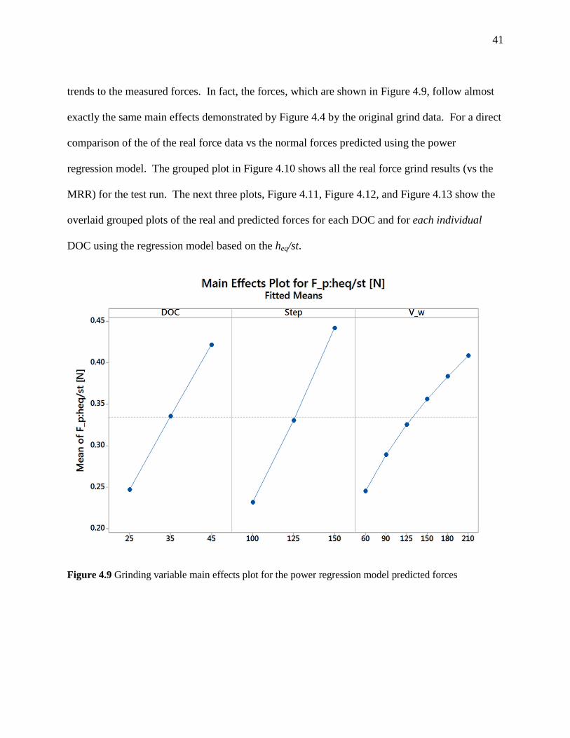
trends to the measured forces. In fact, the forces, which are shown in Figure 4.9, follow almost
exactly the same main effects demonstrated by Figure 4.4 by the original grind data. For a direct
comparison of the of the real force data vs the normal forces predicted using the power
regression model. The grouped plot in Figure 4.10 shows all the real force grind results (vs the
MRR) for the test run. The next three plots, Figure 4.11, Figure 4.12, and Figure 4.13 show the
overlaid grouped plots of the real and predicted forces for each DOC and for each individual
DOC using the regression model based on the heq/st.
Figure 4.9 Grinding variable main effects plot for the power regression model predicted forces

42
Figure 4.10 Grouped plot of the real normal force data vs MRR for the worn wheel
43
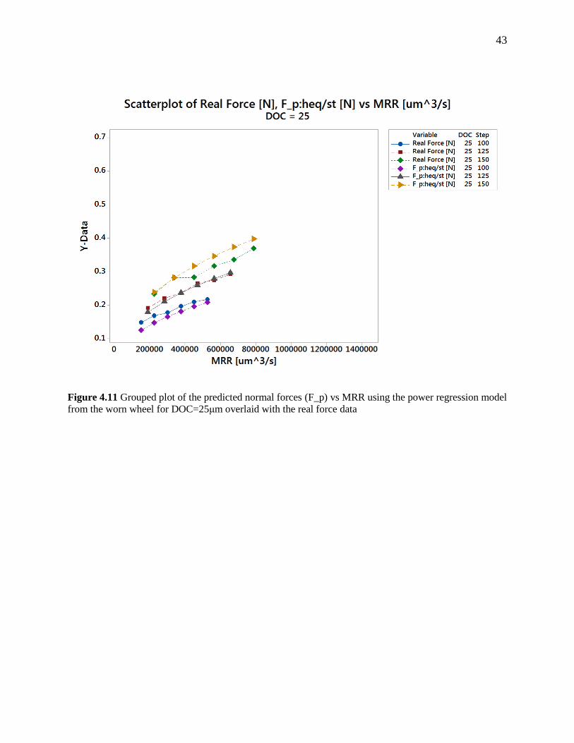
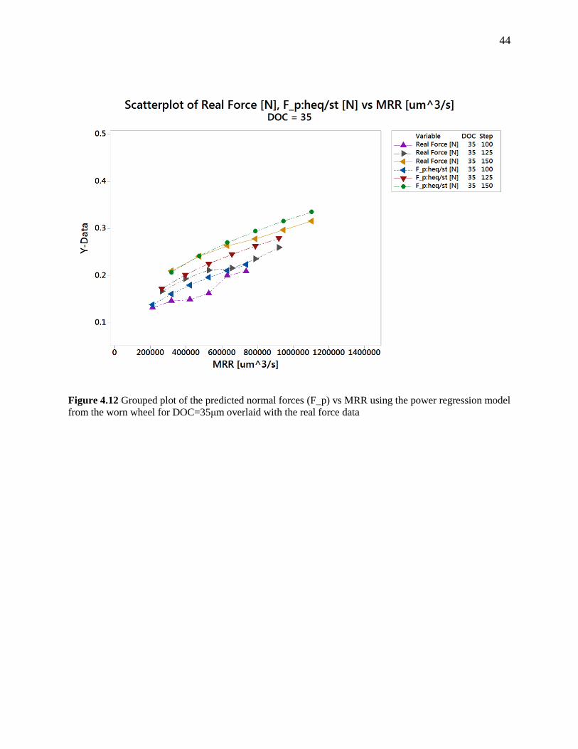
Figure 4.11 Grouped plot of the predicted normal forces (F_p) vs MRR using the power regression model
from the worn wheel for DOC=25μm overlaid with the real force data
44
Figure 4.12 Grouped plot of the predicted normal forces (F_p) vs MRR using the power regression model
from the worn wheel for DOC=35μm overlaid with the real force data

45
Figure 4.13 Grouped plot of the predicted normal forces (F_p) vs MRR using the power regression model
from the worn wheel for DOC=45μm overlaid with the real force data
The similarity between the real and the predicted normal grinding demonstrated in the
overlaid force plots, Figure 4.11 through Figure 4.13, show the fairly good predictive capability
of the power regression model. What the main effects plots for the real and predicted forces
reveal is that the power regression is functionally a smoothed average of all the included data
across all of the grinding variables. This also explains the striking similarity between the main
effects plots (Figure 4.4 and Figure 4.9).
46
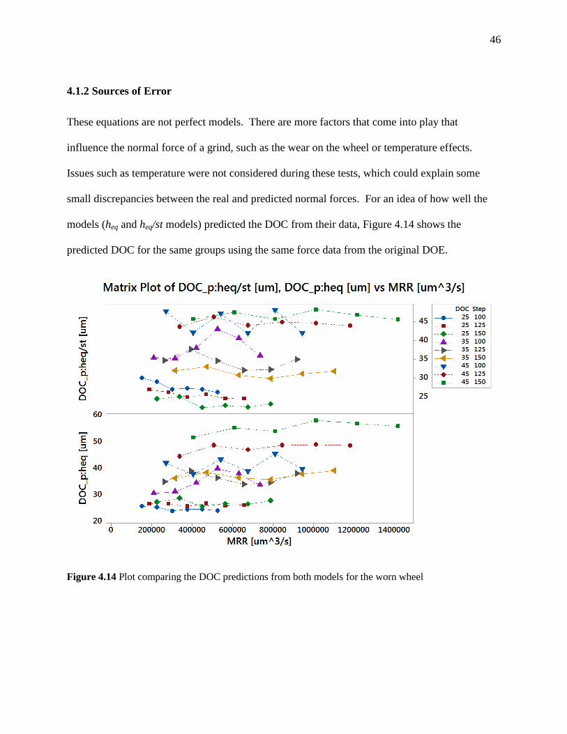
4.1.2 Sources of Error
These equations are not perfect models. There are more factors that come into play that
influence the normal force of a grind, such as the wear on the wheel or temperature effects.
Issues such as temperature were not considered during these tests, which could explain some
small discrepancies between the real and predicted normal forces. For an idea of how well the
models (heq and heq/st models) predicted the DOC from their data, Figure 4.14 shows the
predicted DOC for the same groups using the same force data from the original DOE.
Figure 4.14 Plot comparing the DOC predictions from both models for the worn wheel
47
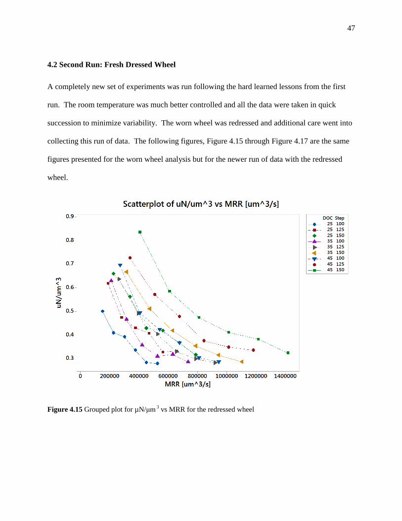
4.2 Second Run: Fresh Dressed Wheel
A completely new set of experiments was run following the hard learned lessons from the first
run. The room temperature was much better controlled and all the data were taken in quick
succession to minimize variability. The worn wheel was redressed and additional care went into
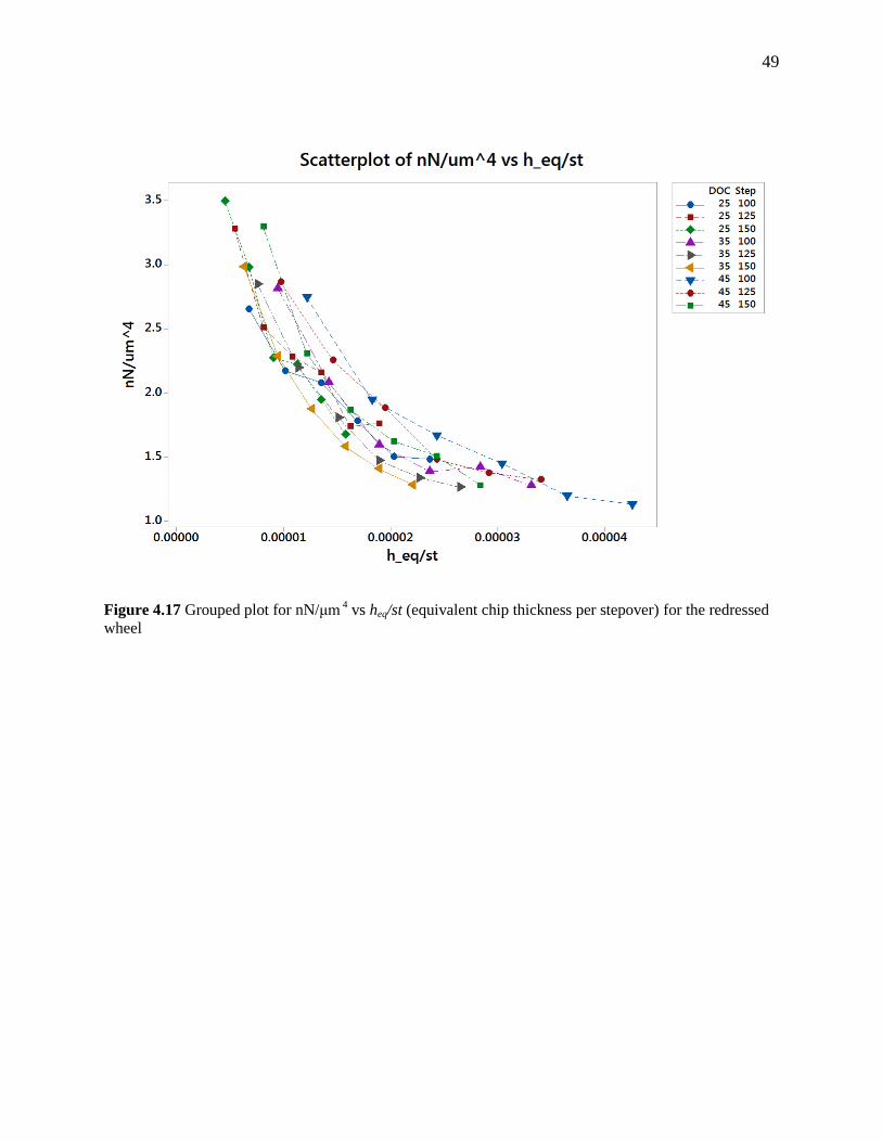
collecting this run of data. The following figures, Figure 4.15 through Figure 4.17 are the same
figures presented for the worn wheel analysis but for the newer run of data with the redressed
wheel.
Figure 4.15 Grouped plot for µN/μm 3 vs MRR for the redressed wheel

48
Figure 4.16 Grouped plot for nN/μm 4 (force per unit volume per length of contact, lc) vs heq for the
redressed wheel
49
Figure 4.17 Grouped plot for nN/μm 4 vs heq/st (equivalent chip thickness per stepover) for the redressed
wheel
50
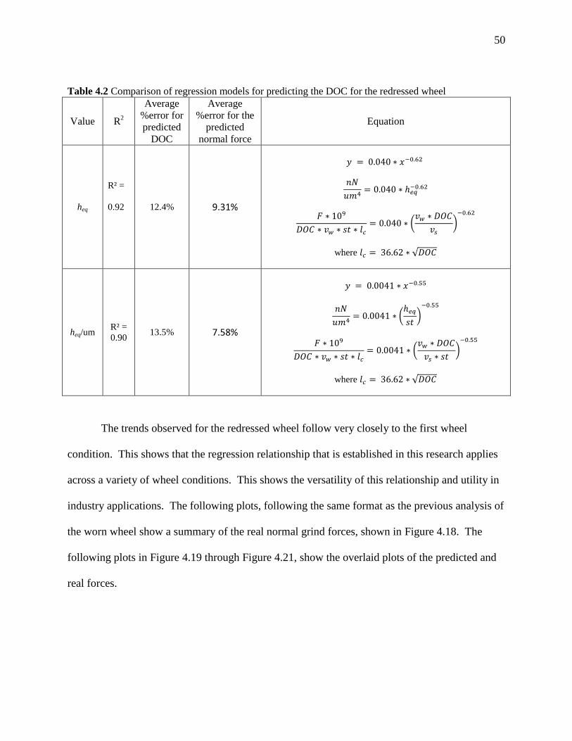
Table 4.2 Comparison of regression models for predicting the DOC for the redressed wheel
Value R2
Average
%error for
predicted
DOC
Average
%error for the
predicted
normal force
Equation
heq
R² =
0.92
12.4% 9.31%
𝑦 = 0.040 ∗ 𝑥−0.62
𝑛𝑁
𝑢𝑚4= 0.040 ∗ ℎ𝑒𝑞
−0.62
𝐹 ∗ 109
𝐷𝑂𝐶 ∗ 𝑣𝑤 ∗ 𝑠𝑡 ∗ 𝑙𝑐
= 0.040 ∗ (𝑣𝑤 ∗ 𝐷𝑂𝐶
𝑣𝑠
)−0.62
where 𝑙𝑐 = 36.62 ∗ √𝐷𝑂𝐶
heq/um R² =
0.90 13.5% 7.58%
𝑦 = 0.0041 ∗ 𝑥−0.55
𝑛𝑁
𝑢𝑚4= 0.0041 ∗ (
ℎ𝑒𝑞
𝑠𝑡)
−0.55
𝐹 ∗ 109
𝐷𝑂𝐶 ∗ 𝑣𝑤 ∗ 𝑠𝑡 ∗ 𝑙𝑐
= 0.0041 ∗ (𝑣𝑤 ∗ 𝐷𝑂𝐶
𝑣𝑠 ∗ 𝑠𝑡)
−0.55
where 𝑙𝑐 = 36.62 ∗ √𝐷𝑂𝐶
The trends observed for the redressed wheel follow very closely to the first wheel
condition. This shows that the regression relationship that is established in this research applies
across a variety of wheel conditions. This shows the versatility of this relationship and utility in
industry applications. The following plots, following the same format as the previous analysis of
the worn wheel show a summary of the real normal grind forces, shown in Figure 4.18. The
following plots in Figure 4.19 through Figure 4.21, show the overlaid plots of the predicted and
real forces.

51
Figure 4.18 Grouped plot of the real normal force data vs MRR for the redressed wheel
52
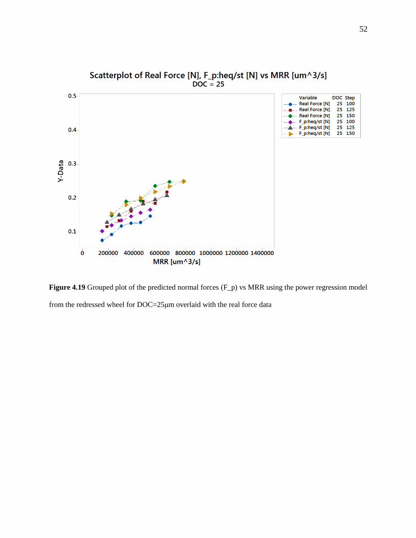
Figure 4.19 Grouped plot of the predicted normal forces (F_p) vs MRR using the power regression model
from the redressed wheel for DOC=25μm overlaid with the real force data

53
Figure 4.20 Grouped plot of the predicted normal forces (F_p) vs MRR using the power regression model
from the redressed wheel for DOC=25μm overlaid with the real force data
54
Figure 4.21 Grouped plot of the predicted normal forces (F_p) vs MRR using the power regression model
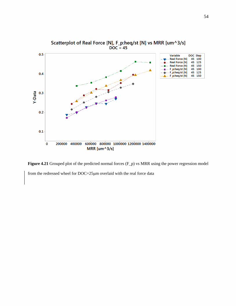
from the redressed wheel for DOC=25μm overlaid with the real force data

55
4.2.1 Sources of Error
The increased error in the regression models shows that there is more to explore on how the
condition of the wheel affects the normal grinding force. A possible error likely occurred while
dressing the wheel and the wheel could have become chipped and therefore not cutting with the
full step. However, the DOC predictions are grouped better (in Figure 4.22) than the previous
data set, in both cases, drawing the conclusion that at least the new data is more consistent.
Figure 4.22 Plot comparing the DOC predictions from both models for the redressed wheel

56
Chapter 5 Additional Observations
5.1 Comparison of the Two Wheels
Evaluating wheel wear is important in industry because if wheel wear can be accurately
predicted, then wheels can be dressed or replaced preemptively. The comparison of these wheels
shows an observable difference between the measured forces for both wheels. These trends are
displayed for ease of interpretation in the main effects plot shown in Figure 5.1. These plots also
show that the effect of the wheel condition has as much of an impact on grinding force as does
changing the grinding parameters. This is a clear and obvious trend and reinforces the ability to
use the power regression to predict the force in grinds to advise when the wheel has been worn
significantly.
Figure 5.1 Plot comparing main effects trends for the force results of both wheels

57
5.2 Zero MRR Rubbing Forces at Depth
When the normal grinding forces are plotted against the MRR, they exhibit a linear trend. This
trend can be traced back to zero to find the vertical axis intercept, which suggests the amount of
force that must be reached before any material is removed from the workpiece, as illustrated in
Figure 5.2 for the redressed wheel. It can also be referred to as the initial force that must be
overcome before the tool begins to remove material as opposed to just rubbing.
Figure 5.2 Grouped plot of normal force vs MRR with regression lines for the redressed wheel
This can be taken a step further by plotting the linear regression values with respect to the
grinding area (the product of the length of contact, lc, and the stepover, st) they form a linear
relationship, shown in Figure 5.3. The first wheel (the worn wheel) has consistently higher zero
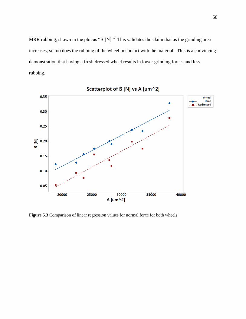
58
MRR rubbing, shown in the plot as “B [N].” This validates the claim that as the grinding area
increases, so too does the rubbing of the wheel in contact with the material. This is a convincing
demonstration that having a fresh dressed wheel results in lower grinding forces and less
rubbing.
Figure 5.3 Comparison of linear regression values for normal force for both wheels
59
5.3 Surface Finish
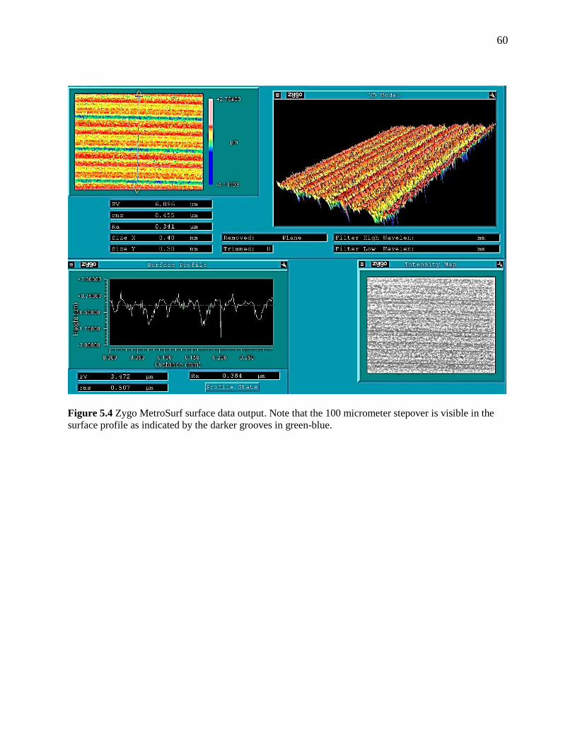
After the samples are ground into the zirconia and the grind force data is collected for the
redressed wheel, the grinding variables were used to grind patches for optical measurement and
then evaluated in the Zygo MetroSurf. The data was analyzed and over the entire range of
grinding variables, the surface roughness Ra was the same ~300 nanometers. A screenshot of the
output is shown in Figure 5.4. In the lower left of the image is a linear surface profile. The
surface profile reveals pits and valleys at are roughly 40-50 μm apart, which is about the same
grit size as the wheel. It may be possible that ~300 nanometers is the best surface that the
grinding wheel of that grit can achieve. This value is acceptable for precision applications where
the dimensional tolerance is the most important factor rather than surface finish. For uses in the
medical industry, much smoother values might be required such as for dental implants. This
requires a finer surface finish, Ra of at least an order of magnitude, which would require a finer
grit size wheel. The grinding parameters may also need to be adjusted to grind the material in
the ductile regime which would produce a completely smooth and reflective surface. Figure 5.5
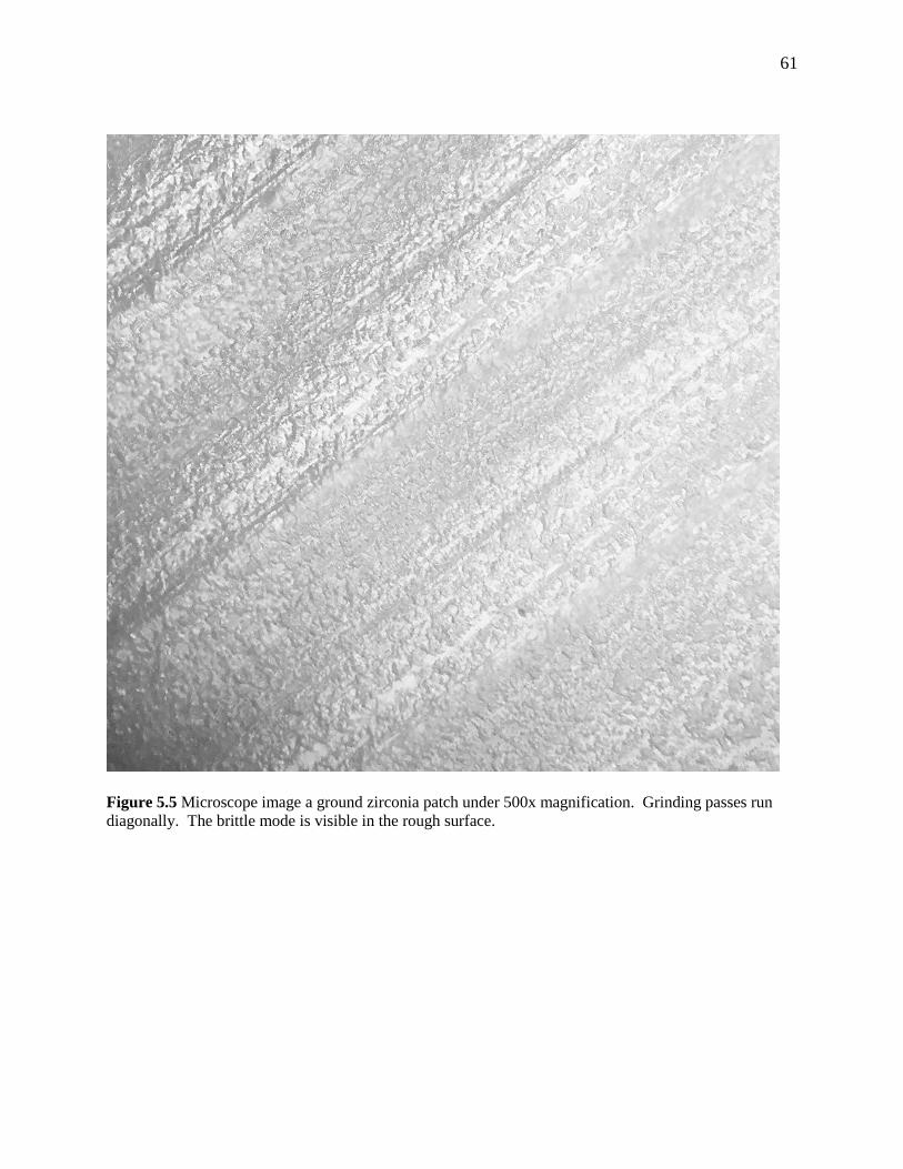
shows a microscope image of a sample patch under 500x magnification. The primarily brittle
grinding mode can be seen from the rough surface of the patch.
60
Figure 5.4 Zygo MetroSurf surface data output. Note that the 100 micrometer stepover is visible in the
surface profile as indicated by the darker grooves in green-blue.
61
Figure 5.5 Microscope image a ground zirconia patch under 500x magnification. Grinding passes run
diagonally. The brittle mode is visible in the rough surface.

62
Chapter 6 Conclusion
This observation of the regression model to predict the DOC based upon the normal force has the
potential to greatly assist with manufacturing processes that involve grinding of small features.
The ability to use force to check the DOC while grinding without manually removing or
inspecting the workpiece would be very beneficial. Equally exciting is the ability to use the
grinding parameters to guess an approximate grinding force for the grind. This can be used to
identify possible failures in the grinding setup, before they incur additional costs in the
manufacturing process, particularly with very small and fragile grinding tools. While the
feedrates in this study were slow compared to most of the research in the literature review, the
current parameters are plenty fast for the machining of features such as small pockets or
microfluidic channels.
Future work, could explore the effect of using a finer grit wheel. A larger set of
machining parameters could also be explored in a better temperature-controlled environment.
The biggest limitation of this work is that the regression relationship must be characterized first
before predictions can be made. However, in the plots of the nN/ μm 4 (the normal force per unit
volume per length of contact, lc), the lines converge around a single power regression. It could
then be possible to take a single set of test cuts using the expected mean of the DOC and
stepover and ramp (or take discreet values) through the expected feedrates. This should be
sufficient to produce the power regression trend. A thorough evaluation should also include an
additional run of tests, in which the wheel is dressed an additional time to determine that the
forces stay approximately the same between the two dressed iterations under identical dressing
parameters. Further work is also required to refine this model to include material and grinding

63
wheel properties to improve the accuracy. The end goal of which is to take a grinding wheel and
material and for a cut with specific parameters, be able to accurately be able to determine
whether the cut was accurate by looking at just the force.

64
Appendix A: Machining Programs
A.1 DressWheel.NC
(Henry Arneson)
(03/30/2016)
(--------------- Truing Diamond Wheel ----------------)
(Linear interpolation)
G01
(ZX Plane lathe)
G18
(tool nose comp off)
G40
G49
(Metric)
G71
(Absolute programming)
G90
(feed per min)
G94
(Wheel At x-contact with soft wheel, just before z-engage)
T0101
(--------------- Program ----------------)
#113 = 0 (offset for troubleshooting)
#114 = -0.040 (previous amount removed)
Z[10] F300
X[10+#113] F100
G04 X02
#171=75 (feed rate)
#100=40 (#number of passes)
#101=0.003 (Depth of each pass)
#102=0 (Start location)
#120=0 (Variable used to calculate the depth of cut)
#131=1 (Pass counter, initially set to 1)
#141=0 (conditional, for finishing passes)
#151=2 (finish passes MUST be even integer)
#161=1 (finish pass counter)
(spindles on)
m03 s1000 (CW)
m03 s2250
G04 X04
Z[5+#114] F50
X[0+#113+#114] F50
G04 X04 (wait)
(adjust pass variable to account for finish passes)
#100=#100-#151/2
(heavier dresses)
while[#131LE#100]do1
(forward cut)
65
#120=#102-[2*#131-1]/2*#101
G01 X[#120+#113+#114] F7
G01 Z-25.000 F[#171]
(reverse cut)
#120=#102-[2*#131]/2*#101
G01 X[#120+#113+#114] F7
G01 Z5.00 F[#171]
#131=#131+1 (update pass counter)
end1
#141=#131-1
(finish dresses)
while[#161LE#151]do2
(forward finish cut)
#120=#102-[#141]*#101-[2*#161-1]*#101/4
G01 X[#120+#113+#114] F5
G01 Z-25.000 F[#171]
(reverse finish cut)
#120=#102-[#141]*#101-[2*#161]*#101/4
G01 X[#120+#113+#114] F5
G01 Z5.00 F[#171]
#161=#161+1
end2
(X[20] F100)
Z[100] F100
(Coolant off)
(m09.1)
m05
m05
m30
66
A.2 FaceZirconia.NC
(This program cup grinds the face of a round zirconia workpiece)
(T0101 at centerline at Z touchoff)
(set grinding wheel to 80 Hz CCW))
(---------- user-defined variables)
#2=-0.055 (starting offset from T0101 [mm])
#12=5 (Z jog offset [mm])
(---------- position/feed variables)
#101=0.001 (axial depth of cut [mm])
#102=20 (number of passes [-])
#103=0 (number of sparkouts)
#107=2 (slow down factor for finishing cuts)
#105=#101/#107 (finishing depth of cut)
(---------- internal variables)
#201=1 (pass counter [-])
#211=0 (current depth [mm])
#212=1 (sparkout counter [-])
#213=0 (sparkout depth)
(---------- program start)
G90 G18 G92.1 G71 G40 (abs, lathe, cancel offset, metric, tool comp off)
M79 (spindle mode)
M03 S317 (CW ISO 5.5 spindle)
T0101 (pick tool 4 furthest out)
G01 Z[#2+#12] F300 (retract position)
G01 X-35
M7 (coolant on)
#102 = #102+1
#7 = 0 (conditional value)
#3 = 1 (loop increment)
WHILE [#201 LE #102] DO1
#7=#201-#102
G01 X-35 F300
(G01 Z[#2] F30)
G01 Z[#2-#211] F30
G01 X-1.0 F25 (adjust center: *-* moves puck away)
(G04 X3)
(IF [#7 LT 1] G04 X10)
G01 Z[#2+#12] F300
#211=#211+#101
#201=#201+#3
END1
(WHILE [#212 LE #103] DO1 )
(G01 X-35 F300)
(G01 Z[#2] F30)
(G01 Z[#2-#213] F30)
(G01 X2.0 F24 (adjust center: *-* moves puck away)
(G01 Z[#2+#12] F300 )
(#212=#212+1)
(END1)
G01 Z[#2+#12] F300 (retract position)
G01 Z50
M9 (coolant off)
M05
M30 (program end)
67
A.3 FaceZirconiaVSandCSS.NC
(This program cup grinds the face of a round zirconia workpiece)
(This utilizes the variable speed and rpm)
(T0101 at centerline at Z touchoff)
(Move the x axis +x mm to create offset for CSS condition)
(REZERO tool at the CSS offset)
(set grinding wheel to 80 Hz CCW))
(---------- user-defined variables)
G94
G97
#2=-0.113 (starting offset from T0101 [mm])
#4=10 (CSS offset *prevents the divide by zero on
RPM)
#12=5 (Z jog offset [mm])
#5=55 (Percent Feed Override)
#21=55 (Cup Wheel radius)
#22=24.5 (Workpiece radius)
#23=3 (Wheel Start offset)
#24=-0.10 (Center offset: *-* moves puck away)
(---------- position/feed variables)
#101=0.001 (axial depth of cut [mm])
#102=50 (Workpiece RPM CW)
#103=0.3 (Feedrate mm/rev *less than wheel edge*)
#104=0.0075 (Final Feedrate mm/rev)
#105=10 (number of passes [-])
#106=5 (Start/Finish speed ratio)
#107=#102*#103*2 (Top Machine Feedrate)
#108=#102*#104 (Low Machine Feedrate)
#110=457 (Inverse Time ms intervals)
#111=#107/60*#110/1000 (Start x travel mm chunk)
#112=#108/60*#110/1000 (Finish x travel mm chunk)
#113=#111-#112 (difference)
(---------- internal variables)
#201=1 (pass counter [-])
#211=0 (current depth [mm])
#212=1 (sparkout counter [-])
#213=0 (sparkout depth)
(---------- program start)
G90 G18 G92.1 G71 G40 (abs, lathe, cancel offset, metric, tool comp off)
G97
M79 (spindle mode)
G94
G04 X1
G94
T0101 (pick tool 4 furthest out)
G94
G01 Z[#2+#12] F300 (retract position)
G01 X[-#22-#12-#4]
G50.6 P[#5]
M7 (coolant on)

68
#102 = #102+1
#7 = 0 (conditional value)
#3 = 1 (loop increment)
#110=#110/1000 (convert to seconds)
M03 S[#102] (CW ISO 5.5 spindle)
G94
WHILE [#201 LE #105] DO1
G50.6 P[100]
G01 X[-#22-#23-#4] F300
(G01 Z[#2] F30)
G01 Z[#2-#211] F30
G50.6 P[#5]
G50 S850
G50 T0101
M03 S[#102] (CW ISO 5.5 spindle)
G01 X[-#22+#24-#4-3] F#107
G96 S[#102]
G95
G01.3
G93 F[#110]
X[-24.5+#24-#4] F[#110]
X[-24.0226+#24-#4] F[#110]
X[-23.5498+#24-#4] F[#110]
X[-23.0818+#24-#4] F[#110]
X[-22.6185+#24-#4] F[#110]
X[-22.1598+#24-#4] F[#110]
X[-21.7059+#24-#4] F[#110]
X[-21.2567+#24-#4] F[#110]
X[-20.8121+#24-#4] F[#110]
X[-20.3723+#24-#4] F[#110]
X[-19.9372+#24-#4] F[#110]
X[-19.5068+#24-#4] F[#110]
X[-19.081+#24-#4] F[#110]
X[-18.66+#24-#4] F[#110]
X[-18.2437+#24-#4] F[#110]
X[-17.8321+#24-#4] F[#110]
X[-17.4252+#24-#4] F[#110]
X[-17.0229+#24-#4] F[#110]
X[-16.6254+#24-#4] F[#110]
X[-16.2326+#24-#4] F[#110]
X[-15.8445+#24-#4] F[#110]
X[-15.4611+#24-#4] F[#110]
X[-15.0823+#24-#4] F[#110]
X[-14.7083+#24-#4] F[#110]
X[-14.339+#24-#4] F[#110]
X[-13.9744+#24-#4] F[#110]
X[-13.6145+#24-#4] F[#110]
X[-13.2593+#24-#4] F[#110]
X[-12.9088+#24-#4] F[#110]
X[-12.5629+#24-#4] F[#110]
69
X[-12.2218+#24-#4] F[#110]
X[-11.8854+#24-#4] F[#110]
X[-11.5537+#24-#4] F[#110]
X[-11.2267+#24-#4] F[#110]
X[-10.9044+#24-#4] F[#110]
X[-10.5868+#24-#4] F[#110]
X[-10.2739+#24-#4] F[#110]
X[-9.9657+#24-#4] F[#110]
X[-9.6622+#24-#4] F[#110]
X[-9.3634+#24-#4] F[#110]
X[-9.0693+#24-#4] F[#110]
X[-8.7799+#24-#4] F[#110]
X[-8.4952+#24-#4] F[#110]
X[-8.2152+#24-#4] F[#110]
X[-7.9399+#24-#4] F[#110]
X[-7.6693+#24-#4] F[#110]
X[-7.4034+#24-#4] F[#110]
X[-7.1422+#24-#4] F[#110]
X[-6.8857+#24-#4] F[#110]
X[-6.6339+#24-#4] F[#110]
X[-6.3868+#24-#4] F[#110]
X[-6.1444+#24-#4] F[#110]
X[-5.9067+#24-#4] F[#110]
X[-5.6737+#24-#4] F[#110]
X[-5.4454+#24-#4] F[#110]
X[-5.2218+#24-#4] F[#110]
X[-5.0029+#24-#4] F[#110]
X[-4.7888+#24-#4] F[#110]
X[-4.5793+#24-#4] F[#110]
X[-4.3745+#24-#4] F[#110]
X[-4.1744+#24-#4] F[#110]
X[-3.979+#24-#4] F[#110]
X[-3.7883+#24-#4] F[#110]
X[-3.6023+#24-#4] F[#110]
X[-3.4211+#24-#4] F[#110]
X[-3.2445+#24-#4] F[#110]
X[-3.0726+#24-#4] F[#110]
X[-2.9054+#24-#4] F[#110]
X[-2.7429+#24-#4] F[#110]
X[-2.5852+#24-#4] F[#110]
X[-2.4321+#24-#4] F[#110]
X[-2.2837+#24-#4] F[#110]
X[-2.14+#24-#4] F[#110]
X[-2.001+#24-#4] F[#110]
X[-1.8668+#24-#4] F[#110]
X[-1.7372+#24-#4] F[#110]
X[-1.6123+#24-#4] F[#110]
X[-1.4922+#24-#4] F[#110]
X[-1.3767+#24-#4] F[#110]
X[-1.2659+#24-#4] F[#110]
X[-1.1598+#24-#4] F[#110]
X[-1.0585+#24-#4] F[#110]
X[-0.9618+#24-#4] F[#110]
X[-0.8698+#24-#4] F[#110]
X[-0.7826+#24-#4] F[#110]
X[-0.7+#24-#4] F[#110]
X[-0.6221+#24-#4] F[#110]
X[-0.549+#24-#4] F[#110]
X[-0.4805+#24-#4] F[#110]
X[-0.4168+#24-#4] F[#110]
X[-0.3577+#24-#4] F[#110]
70
X[-0.3033+#24-#4] F[#110]
X[-0.2537+#24-#4] F[#110]
X[-0.2087+#24-#4] F[#110]
X[-0.1685+#24-#4] F[#110]
X[-0.1329+#24-#4] F[#110]
X[-0.102+#24-#4] F[#110]
X[-0.0759+#24-#4] F[#110]
X[-0.0544+#24-#4] F[#110]
X[-0.0377+#24-#4] F[#110]
X[-0.0256+#24-#4] F[#110]
G04 X0.0
G94 G94
G97 S[#102]
G01 Z[#2+#12] F300
#211=#211+#101
#201=#201+#3
END1
G50.6
G94
G01 Z[#2+#12] F300 (retract position)
G01 X[-50-#4]
G01 Z50
M9 (coolant off)
M05
G94
M30 (program end)
71
A.4 GrindForceSamples.NC
(This program grinds a set of samples for each defined feed speed)
(Set tool 0101 to centerline and touchoff depth *z-touch at radius)
(use force sensor to find touch off position)
(When changing the tool zero, DON'T FORGET TO ALSO CHANGE-)
(THE OPTIONAL LIMITS DEFINED IN THE PROGRAM)
#1=-0.0629 (nominal Z surface location [mm])
#2=2.0 (Z retract during program [mm])
#3=60 (C-axis 0 degree start position [deg])
#4=22.5 (X location for starts)
#19=25 (workpiece radius)
#18=0.75 (wheel edge)
#17=100 (percent feed override)
#29=0.003 (extra depth on the initial path)
#61=30 (feedrate multiplier)
#62=6 (plunge multiplier)
#314=3.14159265358979323
#5=0.045 (sample depth)
#6=1 (sample length [s])
#7=0.150 (sample step)
#8=7 (# of samples)
#9=0.04 (free space between consecutive
samples)
#10=5.5 (3.5,4.5,5.5) (angular dist between sets)
(feedrates: 3,4,5,6,7,8,3 [um/s])
#11=0 (feedrate counter)
#12=6 (# feedrates)
#13=3 (current feedrate, calculated later
[deg/s])
#14=1
#15=1/1000/#4 (first grind speed)
#101=2
#102=3
#103=4
#104=5
#105=6
#106=7
#107=8
#109=1
#150=0.030 (plunge feedrate [mm/min])
#151=300 (fast movements)
(----------- program start)
G90 G18 G92.1 (abs, lathe, cancel offset)
G71 G40 (metric, tool comp off)
G54
G94 G94
M78 (C-axis mode)
T0100
72
G50.3 Z[-206.693999+#1+30] (Z positive limit [mm])
G50.4 Z[-206.693999+#1-0.050] (Z negative limit [mm])
G50.3 X[192.662269]
M50 (engage aux limits)
T0101
G50.6 P[#17]
G01 Z[#1+#2] F100 (retract)
G01 X[#4] (x position for samples)
G01 C[#3] (C position for samples)
M7 (coolant)
#200=0
#11=0
WHILE [#11 LT #12] DO1
#21=#4 (test x position)
#22=#[101+#11]*3/1000/#4*180/#314
#23=#22*#6 (calculate travel)
#24=#23*#8+#9*2
#200=#200+#24
(G01 C[#200] F10)
#11=#11+1
(G04 X1)
END1
(G01 C#200 F10)
IF[#200 GT 360] THEN #1=50
(G01 C[#3+2.5] (find the zero)
(G01 Z[#1+2] F[#151] (find the zero)
(G01 Z[#1+0.010] F5 (find the zero)
(G01 Z[#1-0.035] F[#150] (find the zero)
(G01 Z[#1+#2] F50 (find the zero)
(G04 X10 (find the zero)
#300=0
#11=0
#39=999
WHILE [#11 LT #12] DO1
#31=#4 (keep track of x position)
#32=#3+#9-#300 (keep track of C position)
G01 C[#32]
G01 X[#31]
#33=#[101+#11]*#61/1000/#4*180/#314 (calculate c velocity)
#34=#33*#6
(calculate sample travel)
#35=#34*#8+#9*2
(calculate the full sweep)
#36=#35/#33/100*1000
(calculate time to complete single sample in ms)
#37=fix[#36]/1000
(truncate back to seconds)
73
G01 Z[#1+#2] F#151 (rapid to retract
distance)
G01 Z[#1+0.010] F125 (fast approach)
G01 Z[#1+0.002] F[75] (at surface)
G01 Z[#1-#29-#5] F[#150] (plunge to patch depth)
(G01 C[#32-#35] F[#15] (grind full samples' length)
#37=#37*#18/0.125*2*1.5
#37=#37*1000
#37=fix[#37]/1000
IF [#11 LT 1] THEN #39=#37
G50.6 P[#17]
G94
G01.3
G93 F[#39]
C[#32-0*#35/100] F[#39]
C[#32-1*#35/100] F[#39]
C[#32-2*#35/100] F[#39]
C[#32-3*#35/100] F[#39]
C[#32-4*#35/100] F[#39]
C[#32-5*#35/100] F[#39]
C[#32-6*#35/100] F[#39]
C[#32-7*#35/100] F[#39]
C[#32-8*#35/100] F[#39]
C[#32-9*#35/100] F[#39]
C[#32-10*#35/100] F[#39]
C[#32-11*#35/100] F[#39]
C[#32-12*#35/100] F[#39]
C[#32-13*#35/100] F[#39]
C[#32-14*#35/100] F[#39]
C[#32-15*#35/100] F[#39]
C[#32-16*#35/100] F[#39]
C[#32-17*#35/100] F[#39]
C[#32-18*#35/100] F[#39]
C[#32-19*#35/100] F[#39]
C[#32-20*#35/100] F[#39]
C[#32-21*#35/100] F[#39]
C[#32-22*#35/100] F[#39]
C[#32-23*#35/100] F[#39]
C[#32-24*#35/100] F[#39]
C[#32-25*#35/100] F[#39]
C[#32-26*#35/100] F[#39]
C[#32-27*#35/100] F[#39]
C[#32-28*#35/100] F[#39]
C[#32-29*#35/100] F[#39]
C[#32-30*#35/100] F[#39]
C[#32-31*#35/100] F[#39]
C[#32-32*#35/100] F[#39]
C[#32-33*#35/100] F[#39]
C[#32-34*#35/100] F[#39]
C[#32-35*#35/100] F[#39]
C[#32-36*#35/100] F[#39]
C[#32-37*#35/100] F[#39]
C[#32-38*#35/100] F[#39]
C[#32-39*#35/100] F[#39]
C[#32-40*#35/100] F[#39]
74
C[#32-41*#35/100] F[#39]
C[#32-42*#35/100] F[#39]
C[#32-43*#35/100] F[#39]
C[#32-44*#35/100] F[#39]
C[#32-45*#35/100] F[#39]
C[#32-46*#35/100] F[#39]
C[#32-47*#35/100] F[#39]
C[#32-48*#35/100] F[#39]
C[#32-49*#35/100] F[#39]
C[#32-50*#35/100] F[#39]
C[#32-51*#35/100] F[#39]
C[#32-52*#35/100] F[#39]
C[#32-53*#35/100] F[#39]
C[#32-54*#35/100] F[#39]
C[#32-55*#35/100] F[#39]
C[#32-56*#35/100] F[#39]
C[#32-57*#35/100] F[#39]
C[#32-58*#35/100] F[#39]
C[#32-59*#35/100] F[#39]
C[#32-60*#35/100] F[#39]
C[#32-61*#35/100] F[#39]
C[#32-62*#35/100] F[#39]
C[#32-63*#35/100] F[#39]
C[#32-64*#35/100] F[#39]
C[#32-65*#35/100] F[#39]
C[#32-66*#35/100] F[#39]
C[#32-67*#35/100] F[#39]
C[#32-68*#35/100] F[#39]
C[#32-69*#35/100] F[#39]
C[#32-70*#35/100] F[#39]
C[#32-71*#35/100] F[#39]
C[#32-72*#35/100] F[#39]
C[#32-73*#35/100] F[#39]
C[#32-74*#35/100] F[#39]
C[#32-75*#35/100] F[#39]
C[#32-76*#35/100] F[#39]
C[#32-77*#35/100] F[#39]
C[#32-78*#35/100] F[#39]
C[#32-79*#35/100] F[#39]
C[#32-80*#35/100] F[#39]
C[#32-81*#35/100] F[#39]
C[#32-82*#35/100] F[#39]
C[#32-83*#35/100] F[#39]
C[#32-84*#35/100] F[#39]
C[#32-85*#35/100] F[#39]
C[#32-86*#35/100] F[#39]
C[#32-87*#35/100] F[#39]
C[#32-88*#35/100] F[#39]
C[#32-89*#35/100] F[#39]
C[#32-90*#35/100] F[#39]
C[#32-91*#35/100] F[#39]
C[#32-92*#35/100] F[#39]
C[#32-93*#35/100] F[#39]
C[#32-94*#35/100] F[#39]
C[#32-95*#35/100] F[#39]
C[#32-96*#35/100] F[#39]
C[#32-97*#35/100] F[#39]
C[#32-98*#35/100] F[#39]
C[#32-99*#35/100] F[#39]
C[#32-100*#35/100] F[#39]
G94 G94

75
G01 Z[#1+#2] F100
G04 X6
#51=1
WHILE [#51 LE #8] DO2
#71=0.002
#41=#4-#7
#42=#3-#34*[#51-1]-#300
#45=#34+#9
(calculate the full sample travel)
#46=#45/#33/100*1000 (calculate time to complete
single sample in ms)
#47=fix[#46]/1000
(truncate back to seconds)
#63=#62
IF[#51 LT 2] THEN #63=#62/2
IF[#51 GE 2] THEN #71=#5-0.03
G50.6 P[#17]
G94
G01 X[#41] F50
G01 C[#42] F50
Z01 Z[#1+0.25] F150 (go to predepth)
G01 Z[#1+0.002] F[75] (at surface)
G01 Z[#1-#71] F[10] (go to preplunge depth)
G01 Z[#1-#5] F[#150*#63] (plunge to patch depth)
(G01 C[#42-#45] F[#33] (grind full samples'
length)
G50.6 P[#17]
G01.3
G93 F[#47]
C[#42-0*#45/100] F[#47]
C[#42-1*#45/100] F[#47]
C[#42-2*#45/100] F[#47]
C[#42-3*#45/100] F[#47]
C[#42-4*#45/100] F[#47]
C[#42-5*#45/100] F[#47]
C[#42-6*#45/100] F[#47]
C[#42-7*#45/100] F[#47]
C[#42-8*#45/100] F[#47]
C[#42-9*#45/100] F[#47]
C[#42-10*#45/100] F[#47]
C[#42-11*#45/100] F[#47]
C[#42-12*#45/100] F[#47]
C[#42-13*#45/100] F[#47]
C[#42-14*#45/100] F[#47]
C[#42-15*#45/100] F[#47]
C[#42-16*#45/100] F[#47]
C[#42-17*#45/100] F[#47]
C[#42-18*#45/100] F[#47]
C[#42-19*#45/100] F[#47]
C[#42-20*#45/100] F[#47]
C[#42-21*#45/100] F[#47]
C[#42-22*#45/100] F[#47]
C[#42-23*#45/100] F[#47]
C[#42-24*#45/100] F[#47]
C[#42-25*#45/100] F[#47]
C[#42-26*#45/100] F[#47]
76
C[#42-27*#45/100] F[#47]
C[#42-28*#45/100] F[#47]
C[#42-29*#45/100] F[#47]
C[#42-30*#45/100] F[#47]
C[#42-31*#45/100] F[#47]
C[#42-32*#45/100] F[#47]
C[#42-33*#45/100] F[#47]
C[#42-34*#45/100] F[#47]
C[#42-35*#45/100] F[#47]
C[#42-36*#45/100] F[#47]
C[#42-37*#45/100] F[#47]
C[#42-38*#45/100] F[#47]
C[#42-39*#45/100] F[#47]
C[#42-40*#45/100] F[#47]
C[#42-41*#45/100] F[#47]
C[#42-42*#45/100] F[#47]
C[#42-43*#45/100] F[#47]
C[#42-44*#45/100] F[#47]
C[#42-45*#45/100] F[#47]
C[#42-46*#45/100] F[#47]
C[#42-47*#45/100] F[#47]
C[#42-48*#45/100] F[#47]
C[#42-49*#45/100] F[#47]
C[#42-50*#45/100] F[#47]
C[#42-51*#45/100] F[#47]
C[#42-52*#45/100] F[#47]
C[#42-53*#45/100] F[#47]
C[#42-54*#45/100] F[#47]
C[#42-55*#45/100] F[#47]
C[#42-56*#45/100] F[#47]
C[#42-57*#45/100] F[#47]
C[#42-58*#45/100] F[#47]
C[#42-59*#45/100] F[#47]
C[#42-60*#45/100] F[#47]
C[#42-61*#45/100] F[#47]
C[#42-62*#45/100] F[#47]
C[#42-63*#45/100] F[#47]
C[#42-64*#45/100] F[#47]
C[#42-65*#45/100] F[#47]
C[#42-66*#45/100] F[#47]
C[#42-67*#45/100] F[#47]
C[#42-68*#45/100] F[#47]
C[#42-69*#45/100] F[#47]
C[#42-70*#45/100] F[#47]
C[#42-71*#45/100] F[#47]
C[#42-72*#45/100] F[#47]
C[#42-73*#45/100] F[#47]
C[#42-74*#45/100] F[#47]
C[#42-75*#45/100] F[#47]
C[#42-76*#45/100] F[#47]
C[#42-77*#45/100] F[#47]
C[#42-78*#45/100] F[#47]
C[#42-79*#45/100] F[#47]
C[#42-80*#45/100] F[#47]
C[#42-81*#45/100] F[#47]
C[#42-82*#45/100] F[#47]
C[#42-83*#45/100] F[#47]
C[#42-84*#45/100] F[#47]
C[#42-85*#45/100] F[#47]
C[#42-86*#45/100] F[#47]
C[#42-87*#45/100] F[#47]
77
C[#42-88*#45/100] F[#47]
C[#42-89*#45/100] F[#47]
C[#42-90*#45/100] F[#47]
C[#42-91*#45/100] F[#47]
C[#42-92*#45/100] F[#47]
C[#42-93*#45/100] F[#47]
C[#42-94*#45/100] F[#47]
C[#42-95*#45/100] F[#47]
C[#42-96*#45/100] F[#47]
C[#42-97*#45/100] F[#47]
C[#42-98*#45/100] F[#47]
C[#42-99*#45/100] F[#47]
C[#42-100*#45/100] F[#47]
G94 G94
G01 Z[#1+#2] F[#151] (retract)
G04 X5
#51=#51+1
END2
G04 X10
G01 Z[#1+#2] F25
G01 X[#19] F300
#300=#300+#34*#8+#10
#11=#11+1
END1
G50.5 (cancel aux limits)
M9 (coolant off)
M30 (program end)
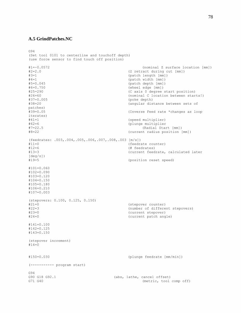
78
A.5 GrindPatches.NC
G94
(Set tool 0101 to centerline and touchoff depth)
(use force sensor to find touch off position)
#1=-0.0572 (nominal Z surface location [mm])
#2=2.0 (Z retract during cut [mm])
#3=1 (patch length [mm])
#4=1 (patch width [mm])
#5=0.045 (patch depth [mm])
#6=0.750 (wheel edge [mm])
#25=290 (C axis 0 degree start position)
#26=60 (nominal C location between starts!)
#37=0.005 (poke depth)
#38=20 (angular distance between sets of
patches)
#39=0.05 (Inverse Feed rate *changes as loop
iterates)
#41=1 (speed multiplier)
#62=6 (plunge multiplier
#7=22.5 (Radial Start [mm])
#8=22 (current radius position [mm])
(feedrates: .003,.004,.005,.006,.007,.008,.003 [m/s])
#11=0 (feedrate counter)
#12=6 (# feedrates)
#13=3 (current feedrate, calculated later
[deg/s])
#19=5 (position reset speed)
#101=0.060
#102=0.090
#103=0.120
#104=0.150
#105=0.180
#106=0.210
#107=0.003
(stepovers: 0.100, 0.125, 0.150)
#21=0 (stepover counter)
#22=3 (number of different stepovers)
#23=0 (current stepover)
#24=0 (current patch angle)
#141=0.100
#142=0.125
#143=0.150
(stepover increment)
#14=0
#150=0.030 (plunge feedrate [mm/min])
(----------- program start)
G94
G90 G18 G92.1 (abs, lathe, cancel offset)
G71 G40 (metric, tool comp off)
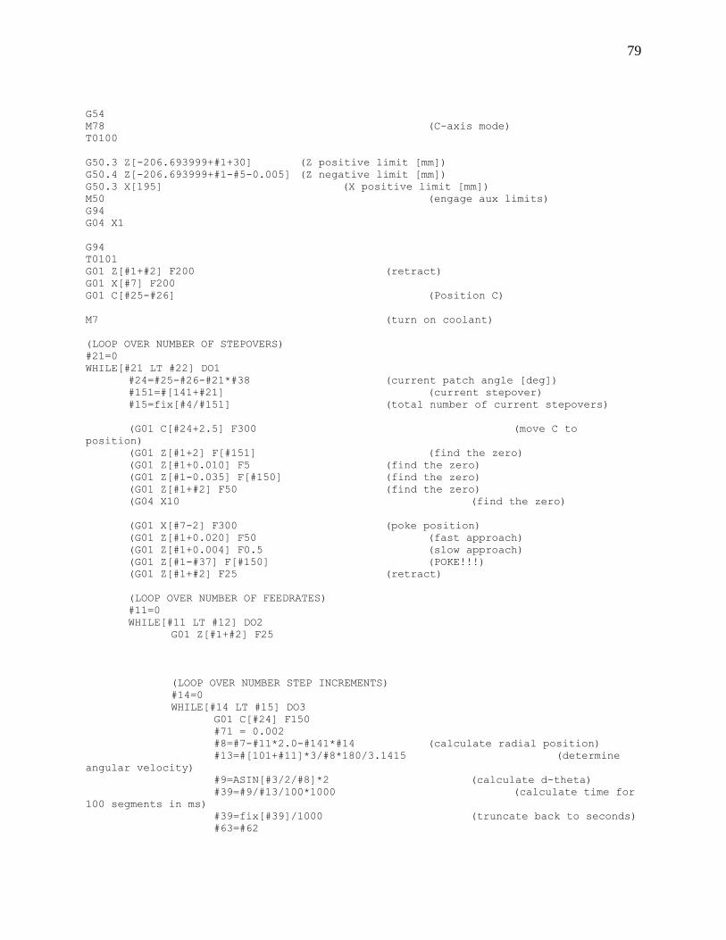
79
G54
M78 (C-axis mode)
T0100
G50.3 Z[-206.693999+#1+30] (Z positive limit [mm])
G50.4 Z[-206.693999+#1-#5-0.005] (Z negative limit [mm])
G50.3 X[195] (X positive limit [mm])
M50 (engage aux limits)
G94
G04 X1
G94
T0101
G01 Z[#1+#2] F200 (retract)
G01 X[#7] F200
G01 C[#25-#26] (Position C)
M7 (turn on coolant)
(LOOP OVER NUMBER OF STEPOVERS)
#21=0
WHILE[#21 LT #22] DO1
#24=#25-#26-#21*#38 (current patch angle [deg])
#151=#[141+#21] (current stepover)
#15=fix[#4/#151] (total number of current stepovers)
(G01 C[#24+2.5] F300 (move C to
position)
(G01 Z[#1+2] F[#151] (find the zero)
(G01 Z[#1+0.010] F5 (find the zero)
(G01 Z[#1-0.035] F[#150] (find the zero)
(G01 Z[#1+#2] F50 (find the zero)
(G04 X10 (find the zero)
(G01 X[#7-2] F300 (poke position)
(G01 Z[#1+0.020] F50 (fast approach)
(G01 Z[#1+0.004] F0.5 (slow approach)
(G01 Z[#1-#37] F[#150] (POKE!!!)
(G01 Z[#1+#2] F25 (retract)
(LOOP OVER NUMBER OF FEEDRATES)
#11=0
WHILE[#11 LT #12] DO2
G01 Z[#1+#2] F25
(LOOP OVER NUMBER STEP INCREMENTS)
#14=0
WHILE[#14 LT #15] DO3
G01 C[#24] F150
#71 = 0.002
#8=#7-#11*2.0-#141*#14 (calculate radial position)
#13=#[101+#11]*3/#8*180/3.1415 (determine
angular velocity)
#9=ASIN[#3/2/#8]*2 (calculate d-theta)
#39=#9/#13/100*1000 (calculate time for
100 segments in ms)
#39=fix[#39]/1000 (truncate back to seconds)
#63=#62
80
IF[#14 LT 1] THEN #39=fix[#39*4*1000]/1000 (1st pass of the
wheel)
IF [#14 GE 1] THEN #71=#5-0.03
IF[#14 LT 1] THEN #63=#62/4
G01 X[#8] F100 (go to radial
position)
G01 Z[#1+0.025] F150 (fast approach)
G01 Z[#1+0.002] F[75] (at surface)
G01 Z[#1-#71] F[10]
G01 Z[#1-#5] F[#150*63] (plunge to patch depth)
(G01 C[#24-#9] F[#13] (Make grind pass)
(#39=#39*10 (speed up for
proofing)
G01.3
G93 F[#39]
C[#24-0*#9/100] F[#39]
C[#24-1*#9/100] F[#39]
C[#24-2*#9/100] F[#39]
C[#24-3*#9/100] F[#39]
C[#24-4*#9/100] F[#39]
C[#24-5*#9/100] F[#39]
C[#24-6*#9/100] F[#39]
C[#24-7*#9/100] F[#39]
C[#24-8*#9/100] F[#39]
C[#24-9*#9/100] F[#39]
C[#24-10*#9/100] F[#39]
C[#24-11*#9/100] F[#39]
C[#24-12*#9/100] F[#39]
C[#24-13*#9/100] F[#39]
C[#24-14*#9/100] F[#39]
C[#24-15*#9/100] F[#39]
C[#24-16*#9/100] F[#39]
C[#24-17*#9/100] F[#39]
C[#24-18*#9/100] F[#39]
C[#24-19*#9/100] F[#39]
C[#24-20*#9/100] F[#39]
C[#24-21*#9/100] F[#39]
C[#24-22*#9/100] F[#39]
C[#24-23*#9/100] F[#39]
C[#24-24*#9/100] F[#39]
C[#24-25*#9/100] F[#39]
C[#24-26*#9/100] F[#39]
C[#24-27*#9/100] F[#39]
C[#24-28*#9/100] F[#39]
C[#24-29*#9/100] F[#39]
C[#24-30*#9/100] F[#39]
C[#24-31*#9/100] F[#39]
C[#24-32*#9/100] F[#39]
C[#24-33*#9/100] F[#39]
C[#24-34*#9/100] F[#39]
C[#24-35*#9/100] F[#39]
C[#24-36*#9/100] F[#39]
C[#24-37*#9/100] F[#39]
C[#24-38*#9/100] F[#39]
C[#24-39*#9/100] F[#39]
C[#24-40*#9/100] F[#39]
C[#24-41*#9/100] F[#39]
C[#24-42*#9/100] F[#39]
C[#24-43*#9/100] F[#39]
81
C[#24-44*#9/100] F[#39]
C[#24-45*#9/100] F[#39]
C[#24-46*#9/100] F[#39]
C[#24-47*#9/100] F[#39]
C[#24-48*#9/100] F[#39]
C[#24-49*#9/100] F[#39]
C[#24-50*#9/100] F[#39]
C[#24-51*#9/100] F[#39]
C[#24-52*#9/100] F[#39]
C[#24-53*#9/100] F[#39]
C[#24-54*#9/100] F[#39]
C[#24-55*#9/100] F[#39]
C[#24-56*#9/100] F[#39]
C[#24-57*#9/100] F[#39]
C[#24-58*#9/100] F[#39]
C[#24-59*#9/100] F[#39]
C[#24-60*#9/100] F[#39]
C[#24-61*#9/100] F[#39]
C[#24-62*#9/100] F[#39]
C[#24-63*#9/100] F[#39]
C[#24-64*#9/100] F[#39]
C[#24-65*#9/100] F[#39]
C[#24-66*#9/100] F[#39]
C[#24-67*#9/100] F[#39]
C[#24-68*#9/100] F[#39]
C[#24-69*#9/100] F[#39]
C[#24-70*#9/100] F[#39]
C[#24-71*#9/100] F[#39]
C[#24-72*#9/100] F[#39]
C[#24-73*#9/100] F[#39]
C[#24-74*#9/100] F[#39]
C[#24-75*#9/100] F[#39]
C[#24-76*#9/100] F[#39]
C[#24-77*#9/100] F[#39]
C[#24-78*#9/100] F[#39]
C[#24-79*#9/100] F[#39]
C[#24-80*#9/100] F[#39]
C[#24-81*#9/100] F[#39]
C[#24-82*#9/100] F[#39]
C[#24-83*#9/100] F[#39]
C[#24-84*#9/100] F[#39]
C[#24-85*#9/100] F[#39]
C[#24-86*#9/100] F[#39]
C[#24-87*#9/100] F[#39]
C[#24-88*#9/100] F[#39]
C[#24-89*#9/100] F[#39]
C[#24-90*#9/100] F[#39]
C[#24-91*#9/100] F[#39]
C[#24-92*#9/100] F[#39]
C[#24-93*#9/100] F[#39]
C[#24-94*#9/100] F[#39]
C[#24-95*#9/100] F[#39]
C[#24-96*#9/100] F[#39]
C[#24-97*#9/100] F[#39]
C[#24-98*#9/100] F[#39]
C[#24-99*#9/100] F[#39]
C[#24-100*#9/100] F[#39]
G04 X0.5
G94
G01 Z[#1+0.025] F100 (fast reverse)
82
IF [#14 LT 20] THEN G04 X2
#14=#14+1 (increment looping
variable)
END3
G01 Z[#1+#2] F200
G01 X[#7] F250
#11=#11+1
END2
#21=#21+1
END1
G50.5 (cancel aux limits)
M9 (coolant off)
M30 (program end)

83
Appendix B: Matlab Programs
B.1 riptextdata.m
function [Time,Force] = riptextdata( filename ) %UNTITLED Summary of this function goes here % Detailed explanation goes here
nCol=2; fid = fopen([filename '.txt'],'r'); firstRowString=fgetl(fid); bla =
textscan(fid,'%f%f','CommentStyle',{'Chan','sec'},'CollectOutput',true); fclose(fid);
data = bla{1}; Time = data(:,1); Force = data(:,2); % s = firstRowString % plot(Time,Force)
end
84
B.2 DataConditioningPlot.m
%superimpose the figures on top of eachother
Hz = 32000; fc = 300; dt = 1/Hz; fs = 1/dt; [b,a] = butter(6,fc/(fs/2));
%Set the rate of decimation for the data r1=20; r2=100; %Select the moving average value n=30;
[x,y]=riptextdata('R35um150umst210umps');
y = detrend(y,'constant');
Ffilt = filter(b,a,y); Ffd1 = decimate(Ffilt,r1); Ffd2 = decimate(Ffilt,r2);
Td1 = (0:1:(length(Ffd1)-1))'*dt*r1; Td2 = (0:1:(length(Ffd2)-1))'*dt*r2;
avgFfd1 = filtfilt(1/n*ones(n,1),1,Ffd1);
n2 = n*r1/r2; avgFfd2 = filtfilt(1/n2*ones(n2,1),1,Ffd2);
% figure(1) % plot(x,y,'r',x,Ffilt,'c',Td1,avgFfd1,'k') % figure(2) plot(x,y,'r',x,Ffilt,'c',Td2,avgFfd2,'k') title('Data Conditioning for Force Samples') xlabel('Time [s]') ylabel('Force [N]') legend('Original','Filtered','Rolling Average')
85
B.3 CupGrindAnalysis.m
%% %This program finds the surface contact ratio as the wheel goes over the %surface of the zirconia puck
clc; clear; clf;
len = 1000;
th = 2; %mm r1 = 55*25.4; %mm radius wheel r2 = 1*25.4; %mm radius Zirconia puck
rad = linspace(0,r2,len); travel = linspace((r1+r2),r1,len); x = zeros(1,length(travel)); ang = zeros(1,length(travel)); arcl = zeros(1,length(travel));
for j=1:length(travel) bla = (r1^2-r2^2-travel(j)^2)/(2*travel(j)); x(j) = bla; Y = (sqrt(r2^2-(x(j))^2)); X = (x(j)+travel(j)); ang(j) = atan2(abs(Y),X); arcl(j) = 2*ang(j)/(2*pi)*2*r1*pi; end
plot(rad,arcl) title('Contact Length of Grinding Wheel') xlabel('Radius Location [mm]') ylabel('Contact Length [mm]')
%% %This section finds the grind travel for each point on the radius stp = 0.1; r=linspace(r2,stp,len); omega = 300; vw = omega*2*pi/60; gl = zeros(1,len); tgrind = 30;
for m=1:length(gl) gl(m) = r(m).*vw*tgrind; end
figure(2) plot(r,gl)

86
title('Radius Travel While Engaged with Grinding Wheel') xlabel('Point on Radius [mm]') ylabel('Travel [mm]')
%% %This section compares all of the different cup grinding scenarios
omega = 300; %rev/min feedrate = 30; %mm/min stp = feedrate/omega; %mm/rev
% len = 1000;
r=linspace(r2,stp,len); dr = zeros(1,length(r)); drVF = zeros(1,length(r));
a = 0.3; %initial speed mm/rev b = 0.0075; %final speed mm/rev s1 = 211; s2 = 750;
offset = 10;
for la=1:len drpm(la) = s1*(r2+offset)/(r(la)+offset); drpmX(la) = s1*(r2+offset)/(r(la)); end
s2 = drpm(end) sIDEAL = drpmX(end)
hs = a*omega/60; %mm/s ls = b*omega/60; %mm/s sdif = linspace(hs,ls,len)*.55; sdifX = linspace(hs,ls,len); % drpm = linspace(s1,s2,len);
dt = r./sdif; dtx = r./sdifX;
for k=1:length(r) dr(k) = 2*r(k)*omega*2*pi/60*r(k)/feedrate*60;
drVF(k) = 2*r(k)*omega*2*pi/60*dt(k);
drVFCSS(k) = 2*r(k)*drpm(k)*2*pi/60*dt(k);
drIDEAL(k) = 2*r(k)*drpmX(k)*2*pi/60*dtx(k);
87
end
figure(3) plot(r,dr,'b',r,drVF,'g',r,drVFCSS,'r',r,drIDEAL,'k') legend('Original Traverse','Variable Feed','Variable Feed and RPM','Ideal
Conditions') title('Simulation of Cup Grinding Conditions') xlabel('Point on Radius [mm]') ylabel('Travel [mm]')
88
B.4 PredictDOCusingh_eq.m
%% %This program uses the real force values and the given grinding %parameters, solves the regression model (for h_eq) for the DOC
clear; clc;
NF=[ 0.075106974 0.092231363 0.117707072 0.126044766 0.127713652 0.14673398 0.11600141 0.133296572 0.161509573 0.190960262 0.184483969 0.218115792 0.148494727 0.189825057 0.193091658 0.235877695 0.247973567 0.249232387 ];
syms F d t w s
r = 500*sqrt(2);
left = (F*10^9)/(d*w*t)/(36.62329818*d^0.509468544); right = 0.040281055*(w/s*d)^(-0.61644787);
pdoc = 25; %[20;35;45]; %25:10:45; pstep = 100:25:150; pspeed = 60:30:210; ndoc = length(pdoc); nstep = length(pstep); nspeed = length(pspeed); Vs = 2221441; spRange = 10; docRes = 0.01;
doc = (pdoc(1)-spRange):docRes:(pdoc(1)+spRange); acc = 0.1;
89
err = zeros(1,length(doc)); % leftEval = zeros(1,length(doc)); % rightEval = leftEval; docG = zeros((ndoc*nstep*nspeed),1);
for m=1:ndoc for k=1:nstep for o=1:nspeed doc = (pdoc(m)-spRange):docRes:(pdoc(m)+spRange); counter = (m-1)*nstep*nspeed+(k-1)*nspeed+(o-1)+1 currdoc = pdoc(m); currstep = pstep(k); currspeed = pspeed(o); currForce = NF(counter); n=1; curErr=5; while n<=length(doc)%curErr >= acc leftEval =
eval(subs(subs(subs(subs(left,'d',doc(n)),'w',pspeed(o)),'t',pstep(k)),'F',NF
(counter))); rightEval =
eval(subs(subs(subs(subs(right,'d',doc(n)),'w',pspeed(o)),'t',pstep(k)),'s',V
s)); err(n) = abs(leftEval-rightEval); curErr = err(n); % if n==length(doc) % docG(counter) = NaN; % n=n-1; % break; % end; n=n+1; end
bla = doc(err == min(err)) docG(counter) = bla; end end end % doc(n) % plot(err)
plot(doc,leftEval,'k',doc,rightEval,'b') % plot(doc,rightEval,'b')
% end
90
B.5 Predict DOCusingh_eqdst.m
%% %This program uses the real force values and the given grinding %parameters, solves the regression model (for h_eq/um) for the DOC
clear; clc;
NF=[ 0.075106974 0.092231363 0.117707072 0.126044766 0.127713652 0.14673398 0.11600141 0.133296572 0.161509573 0.190960262 0.184483969 0.218115792 0.148494727 0.189825057 0.193091658 0.235877695 0.247973567 0.249232387 ];
syms F d t w s
r = 500*sqrt(2);
left = (F*10^9)/(d*w*t)/(36.62329818*d^0.509468544); right = 0.00413773*(w/s*d/t)^(-0.55169791);
pdoc = 25; %[20;35;45]; %25:10:45; pstep = 100:25:150; pspeed = 60:30:210; ndoc = length(pdoc); nstep = length(pstep); nspeed = length(pspeed); Vs = 2221441; spRange = 10; docRes = 0.01;
doc = (pdoc(1)-spRange):docRes:(pdoc(1)+spRange); acc = 0.1;

91
err = zeros(1,length(doc)); % leftEval = zeros(1,length(doc)); % rightEval = leftEval; docG = zeros((ndoc*nstep*nspeed),1);
for m=1:ndoc for k=1:nstep for o=1:nspeed doc = (pdoc(m)-spRange):docRes:(pdoc(m)+spRange); counter = (m-1)*nstep*nspeed+(k-1)*nspeed+(o-1)+1 currdoc = pdoc(m); currstep = pstep(k); currspeed = pspeed(o); currForce = NF(counter); n=1; curErr=5; while n<=length(doc)%curErr >= acc leftEval =
eval(subs(subs(subs(subs(left,'d',doc(n)),'w',pspeed(o)),'t',pstep(k)),'F',NF
(counter))); rightEval =
eval(subs(subs(subs(subs(right,'d',doc(n)),'w',pspeed(o)),'t',pstep(k)),'s',V
s)); err(n) = abs(leftEval-rightEval); curErr = err(n); % if n==length(doc) % docG(counter) = NaN; % n=n-1; % break; % end; n=n+1; end
bla = doc(err == min(err)) docG(counter) = bla; end end end % doc(n) % plot(err)
plot(doc,leftEval,'k',doc,rightEval,'b') % plot(doc,rightEval,'b')
% end

92
B.6 Force Extraction Programs in report form.m
%% %This program uses the previous method of conditioning the data and loops %over all the provided samples in a specific group and extracts all the %force values and then averages them for a set of grinding parameters
clear all clf clc
Hz = 32000; %Sampling Rate of the DataPhysics box l = 8*Hz; %length of extracted samples sl = 1*Hz; %length of individual grinds in samples
files = {'R45um125umst60umps' 'R45um125umst90umps' 'R45um125umst120umps'
'R45um125umst150umps' 'R45um125umst180umps' 'R45um125umst210umps' }; starts = 00*ones(length(files),1); starts = starts + round(-
170*Hz+Hz*[217.859895291363;216.988732440167;217.905745967742;215.75076417794
0;216.759479058273;216.652494146722]); pstart = round(-
l/2+Hz.*[39.2741935483871;71.5322580645161;104.112903225806;136.532258064516;
168.951612903226])'; %select using the ginput % %select pstarts at the start of each mini-grind
%change the vertical stagger of data stack = 0.5; subs = 1; speeds = length(files); trim = 200*Hz; samples = [1 2 3 4 5]; %mm/s plunges = length(samples); titles = {'60 um/s';'90 um/s';'120 um/s';'150 um/s';'180 um/s';'210 um/s'};
%Make Filter fc = 300; dt = 1/Hz; fs = 1/dt; [b,a] = butter(6,fc/(fs/2));
%Set the rate of decimation for the data r=100; %Select the moving average value n=7;
datas = zeros(round(trim/r),1);
figure(1) hold on for outer = 1: length(files), fnum = outer;
93
[t,data]=riptextdata(files{fnum});
%massage the data into more manageable stuff data = detrend(data, 'constant'); data = filter(b,a,data); data = decimate(data,r); trimd = round(trim/r);
%trim the data data = data(round(starts(outer)/r)+(1:trimd)); t = (0:1:(length(data)-1))'*dt*r;
%apply rolling average data = filtfilt(1/n*ones(n,1),1,data);
% % % remove gravity % % tfit = t([(1:300), (end-300+1:end)]); % % tdx = data([(1:300), (end-300+1:end)],1); % % % tdy = data([(1:50), (end-50+1:end)],2); % % snfit=polyfit(tfit, tdx, 1); % % % stfit=polyfit(tfit, tdy, 1);
% % % data(:,1) = data(:,1) - polyval(snfit,t); % % % % data(:,2) = data(:,2) - polyval(stfit,t);
plot(t, data + stack*(outer-1)) datas = horzcat(datas,data); hold on
% % use once % plot(t, data) % henry(outer,:)=ginput(1); % pause(0.1) end
% [grindstarts,y] = ginput(length(samples));
datas = datas(:,2:end);
%split the data into the four separate plunge grinds l = round(l/r); gstart = 1; gend = gstart+l; t_step = t(2)-t(1); pass = zeros(gend-gstart+1,speeds); pstart = round(pstart./r);
gds = 0.45; %seconds in the grinding force to use for the mean gds = round(gds*Hz/r);
% graphTop = 0.4;

94
stack = 0; gravityends = 25;
figure(2) hold on
endS = 2; %# of seconds at ends of extracted samples %to use to remove temperature effects endP = round(endS*Hz/r); sl = round(sl/r);
tops = zeros(length(samples),speeds);
for a=1:speeds for b=1:length(samples) %select individual grinds datap = datas(pstart(b)+(gstart:gend),a); tpass = t(1:gend); % % datap = detrend(datap,'constant'); datap = detrend(datap,'constant'); tfit = tpass([(1:endP), (end-endP+1:end)]); Ffit = datap([(1:endP), (end-endP+1:end)]); snfit=polyfit(tfit,Ffit,3); datap = datap-polyval(snfit,tpass); pass(:,b) = datap; srise = find(datap>(max(datap)*0.65)); srise = srise(1);
forcesample = datap(srise+sl/4+(1:gds)); tsample = tpass(srise+sl/4+(1:gds)); tops(b,a) = mean(forcesample); if a==1 graphTop = tops(b,a)*1.75; end
subplot(1,speeds,a) hold on plot(tpass,pass(:,b),tsample,forcesample,'rx') % plot(tsample,forcesample,'rx') axis([0 tpass(end) -graphTop graphTop])
end
axis([0 tpass(end) -graphTop/5 graphTop]) title(titles(a)) xlabel('Time (s)') ylabel('Force (N)') end hold off
forceavg = mean(tops,1)';

95
References
[1] W. B. Rowe, "Basic Material Removal," in Principles of Modern Grinding Technology
Second Edition, Liverpool, Elsevier Inc., 2014, pp. 15-33.
[2] W. B. Rowe, Principles of Modern Grinding Technology Second Edition, Liverpool: Elsevier
Inc., 2014.
[3] R. Snoeys and J. Peters, "The significance of chip thickness in grinding," Research Center of
the Belgian Metalworking Industry, Leuven, 1984.
[4] M. Rabiey, N. Jochum and F. Kuster, "High performance grinding of circonium oxide (ZrO2)
using hybrid bond diamond tools," CIRP Annals - Manufacturing Technology, vol. 62, pp.
343-346, 2013.
[5] W. B. Rowe, "Introduction," in Principles of Modern Grinding Technology Second Edition,
Liverpool, Elsevier Inc., 2014, pp. 2-13.
[6] W. B. Rowe, "High Speed Grinding," in Principles of Modern Grinding Technology Second
Edition, Liverpool, Elsevier Inc., 2014, pp. 101-112.
[7] B. R. Knapp, "Master's Thesis: Benefits of Grinding with Variable Workspeed," The
Pennsylvania State University: The Graduate School College of Engineering, University
Park, 1999.
[8] B. R. Knapp, "PhD Thesis: On the Use of an Instrumented Spindle to Determine the Effects
of Machine Stiffness in Grinding Brittle Materials," The Pennsylvania State University: The
Graduate School College of Engineering, University Park, 2002.

96
[9] T. R. S. Deakyne, "PhD Thesis: Study of the Relationship between Machine Compliance and
Grinding Forces in Cylindrical Grinding," The Pennsylvania State University: The Graduate
School College of Engineering, University Park, 2012.

![Formation characterization and rheological properties of ... · of rheology is of paramount importance for zirconia and partially stabilized zirconia [33-35], especially when stabilization](https://img.pdfslide.us/doc/110x75/5e513efd0343e320cf1e4764/formation-characterization-and-rheological-properties-of-of-rheology-is-of-paramount.jpg)