Embed Size (px)
Citation preview

S D P SSurface Deformation Prediction System
for Windowsversion 5.2
Quick Reference Guide and Working Examples
by
Dr. Zacharias Agioutantis and Dr. Michael KarmisDepartment of Mining and Minerals Engineering
Virginia Polytechnic Institute and State UniversityBlacksburg, Virginia 24061-0239
This software package is the property of the Department ofMining and Minerals Engineering, VPI & SU. It has been licensedand may be distributed only to O.S.M.R.E. and State RegulatoryAgencies. The SDPS software can be purchased by individuals
and/or companies through Carlson Software.
February 2002

SDPS Quick Reference Guide, February 2002 2
DisclaimerThe authors declare that there are no warranties,expressed or implied, which apply to the softwarecontained herein. By acceptance and use of saidsoftware, which is conveyed to the user without
consideration by the authors, the user hereof expresslywaives any and all claims for damage and/or suits foror by reason of personal injury, or property damage,
including special, consequential or other similardamages arising out of or in any way connected with
the use of the software contained herein.

SDPS Quick Reference Guide, February 2002 3
The purpose of this guide is to provide a quickreference guide to the SDPS for windows (version 5.x)suite of programs and to develop working experiencethrough the application of examples. This guide is notdesigned to be a tutorial in ground control engineeringor in subsidence engineering. It is assumed that the
user is already familiar with the basic principles ofground deformation prediction and pillar stability
evaluation.
As of version 5.1, the SDPS suite of programs includesthe Pillar Stability Analysis programs (ALPS and
ARMPS) developed by NIOSH.

SDPS Quick Reference Guide, February 2002 4
Table of Contents
Chapter 1: Introduction . . . . . . . . . . . . . . . . . . . . . . . . . . . . . . . . . . . . . . . . . . . . . . . . 111.1 Requirements . . . . . . . . . . . . . . . . . . . . . . . . . . . . . . . . . . . . . . . . . . . . . . . 131.2 Installing / UnInstalling SDPS . . . . . . . . . . . . . . . . . . . . . . . . . . . . . . . . . . 14
1.2.1 Installing from a CDROM . . . . . . . . . . . . . . . . . . . . . . . . . . . . . . 141.2.2 Installing from diskettes . . . . . . . . . . . . . . . . . . . . . . . . . . . . . . . 141.2.3 Registration . . . . . . . . . . . . . . . . . . . . . . . . . . . . . . . . . . . . . . . . . 141.2.4 Uninstalling . . . . . . . . . . . . . . . . . . . . . . . . . . . . . . . . . . . . . . . . . 14
1.3 SDPS Software Overview . . . . . . . . . . . . . . . . . . . . . . . . . . . . . . . . . . . . . 151.4 SDPS Features . . . . . . . . . . . . . . . . . . . . . . . . . . . . . . . . . . . . . . . . . . . . . 161.5 General Configuration of the SDPS Programs . . . . . . . . . . . . . . . . . . . . . 171.6 Custom Configuration of the SDPS Programs . . . . . . . . . . . . . . . . . . . . . . 181.7 Overview of Subsidence Parameters . . . . . . . . . . . . . . . . . . . . . . . . . . . . . 19
Chapter 2: The Profile Function Method . . . . . . . . . . . . . . . . . . . . . . . . . . . . . . . . . . 222.1 Overview of the Profile Function Method . . . . . . . . . . . . . . . . . . . . . . . . . . 222.2 Example #1: Calculations Using the Profile Function Program . . . . . . . . . 242.3 Example #2: Setting the Basic Graph Options - Profile Function
Method . . . . . . . . . . . . . . . . . . . . . . . . . . . . . . . . . . . . . . . . . . . . . . . . . 272.4 Example #3: Working with the Advanced Graphics Options - Profile
Function Method . . . . . . . . . . . . . . . . . . . . . . . . . . . . . . . . . . . . . . . . . . 29
Chapter 3: The Influence Function Method . . . . . . . . . . . . . . . . . . . . . . . . . . . . . . . . 313.1 Overview of the Influence Function Method . . . . . . . . . . . . . . . . . . . . . . 313.2 Definition of the Mine Plan in the Influence Function Program . . . . . . . . . 373.3 Definition of the Prediction Points in the Influence Function Program . . . . 403.4 Example #4: Calculations Using the Influence Function Program -
Deformations on a Transverse Line . . . . . . . . . . . . . . . . . . . . . . . . . . . 413.5 Example #5: Calculations Using the Influence Function Program -
Adjusting the Panel Boundaries . . . . . . . . . . . . . . . . . . . . . . . . . . . . . . 453.6 Example #6: Calculations Using the Influence Function Program -
Deformations Around a Panel Edge . . . . . . . . . . . . . . . . . . . . . . . . . . . 473.7 Example #7: Calculations Using the Influence Function Program -
Deformations over Two Longwall Panels . . . . . . . . . . . . . . . . . . . . . . . 493.8 Example #8: Calculations Using the Influence Function Program -
Deformations over a Room-and-Pillar Section with a RemnantStable Pillar . . . . . . . . . . . . . . . . . . . . . . . . . . . . . . . . . . . . . . . . . . . . . . 52
3.9 Example #9: Calculations Using the Influence Function Program -Strains on Pipeline over a Longwall Panel . . . . . . . . . . . . . . . . . . . . . . 54
3.10 Example #10: Calculations Using the Influence Function Program -Deformations due to Multiple Seam Mining . . . . . . . . . . . . . . . . . . . . . 56
3.11 Example #11: Calculations Using the Influence Function Program -Deformations on a line over a Room & Pillar Section . . . . . . . . . . . . . . 57

SDPS Quick Reference Guide, February 2002 5
3.12 Example #12: Calculations Using the Influence Function Program -Deformations over a Room & Pillar Section Using Data fromAutoCAD / SurvCADD . . . . . . . . . . . . . . . . . . . . . . . . . . . . . . . . . . . . . . 59
3.13 Example #13: Calculations Using the Influence Function Program -Develop Site Specific Subsidence Predictions Using Known FieldData . . . . . . . . . . . . . . . . . . . . . . . . . . . . . . . . . . . . . . . . . . . . . . . . . . . . 62
3.14 Example #14: Site Specific Parameters for a Room-and-Pillar CaseStudy - Influence Function method . . . . . . . . . . . . . . . . . . . . . . . . . . . . 64
Chapter 4: Pillar Stability Analysis Calculations . . . . . . . . . . . . . . . . . . . . . . . . . . . . . 754.1 Pillar Design for Room and Pillar Operations . . . . . . . . . . . . . . . . . . . . . . 754.2 The ALPS Method . . . . . . . . . . . . . . . . . . . . . . . . . . . . . . . . . . . . . . . . . . . 764.3 The ARMPS Method . . . . . . . . . . . . . . . . . . . . . . . . . . . . . . . . . . . . . . . . . 794.3 Example #15: Calculations Using the Pillar Stability Analysis Module -
Estimation of Pillar Safety Factors . . . . . . . . . . . . . . . . . . . . . . . . . . . . 824.4 Example #16: Calculations Using the Pillar Stability Analysis Module -
Estimation of Protection Area . . . . . . . . . . . . . . . . . . . . . . . . . . . . . . . . 854.5 Example #17: Calculations Using the ALPS Module - Estimation of
ALPS Stability Factors . . . . . . . . . . . . . . . . . . . . . . . . . . . . . . . . . . . . . 874.6 Example #18: Calculations Using the ARMPS Module - Estimation of
ARMPS Stability Factors . . . . . . . . . . . . . . . . . . . . . . . . . . . . . . . . . . . . 90
Chapter 5: The Graphing Module . . . . . . . . . . . . . . . . . . . . . . . . . . . . . . . . . . . . . . . . 935.1 Two-Dimensional Images: Cross-sectional plots . . . . . . . . . . . . . . . . . . . . 935.2 Two-Dimensional Images: Vector plots . . . . . . . . . . . . . . . . . . . . . . . . . . . 945.3 Three-Dimensional Images . . . . . . . . . . . . . . . . . . . . . . . . . . . . . . . . . . . . 94
Chapter 6: References . . . . . . . . . . . . . . . . . . . . . . . . . . . . . . . . . . . . . . . . . . . . . . . . 95
Appendix 1: Program Reference . . . . . . . . . . . . . . . . . . . . . . . . . . . . . . . . . . . . . . . . 98A1.1 The Profile Function Module . . . . . . . . . . . . . . . . . . . . . . . . . . . . . . . . . . 99
A1.1.1 The File Menu . . . . . . . . . . . . . . . . . . . . . . . . . . . . . . . . . . . . . . 99A1.1.2 The Edit Menu . . . . . . . . . . . . . . . . . . . . . . . . . . . . . . . . . . . . . 100A1.1.3 The Utilities Menu . . . . . . . . . . . . . . . . . . . . . . . . . . . . . . . . . . 103
A1.2 The Influence Function Module . . . . . . . . . . . . . . . . . . . . . . . . . . . . . . . 106A1.2.1 The File Menu . . . . . . . . . . . . . . . . . . . . . . . . . . . . . . . . . . . . . 106A1.2.2 The Edit Menu . . . . . . . . . . . . . . . . . . . . . . . . . . . . . . . . . . . . . 110A1.2.3 The Calculate Menu . . . . . . . . . . . . . . . . . . . . . . . . . . . . . . . . . 115A1.2.4 The Utilities Menu . . . . . . . . . . . . . . . . . . . . . . . . . . . . . . . . . . 118
A1.3 The Pillar Stability Module . . . . . . . . . . . . . . . . . . . . . . . . . . . . . . . . . . . 120A1.3.1 The File Menu . . . . . . . . . . . . . . . . . . . . . . . . . . . . . . . . . . . . . 120A1.3.2 The Edit Menu . . . . . . . . . . . . . . . . . . . . . . . . . . . . . . . . . . . . . 120A1.3.3 The Output Menu . . . . . . . . . . . . . . . . . . . . . . . . . . . . . . . . . . . 121A1.3.4 The Utilities Menu . . . . . . . . . . . . . . . . . . . . . . . . . . . . . . . . . . 122
A1.4 The ALPS Module . . . . . . . . . . . . . . . . . . . . . . . . . . . . . . . . . . . . . . . . . 124A1.4.1 The File Menu . . . . . . . . . . . . . . . . . . . . . . . . . . . . . . . . . . . . . 124

SDPS Quick Reference Guide, February 2002 6
A1.4.2 The Edit Menu . . . . . . . . . . . . . . . . . . . . . . . . . . . . . . . . . . . . . 124A1.4.3 The Output Menu . . . . . . . . . . . . . . . . . . . . . . . . . . . . . . . . . . . 125A1.4.4 The Utilities Menu . . . . . . . . . . . . . . . . . . . . . . . . . . . . . . . . . . 126
A1.5 The ARMPS Module . . . . . . . . . . . . . . . . . . . . . . . . . . . . . . . . . . . . . . . 128A1.5.1 The File Menu . . . . . . . . . . . . . . . . . . . . . . . . . . . . . . . . . . . . . 128A1.5.2 The Edit Menu . . . . . . . . . . . . . . . . . . . . . . . . . . . . . . . . . . . . . 128A1.5.3 The Output Menu . . . . . . . . . . . . . . . . . . . . . . . . . . . . . . . . . . . 129A1.5.4 The Utilities Menu . . . . . . . . . . . . . . . . . . . . . . . . . . . . . . . . . . 129
A1.6 The Graph Module . . . . . . . . . . . . . . . . . . . . . . . . . . . . . . . . . . . . . . . . 131A1.6.1 The File Menu . . . . . . . . . . . . . . . . . . . . . . . . . . . . . . . . . . . . . 131A1.5.2 The 2-D Menu . . . . . . . . . . . . . . . . . . . . . . . . . . . . . . . . . . . . . 131A1.6.3 The 3-D Menu . . . . . . . . . . . . . . . . . . . . . . . . . . . . . . . . . . . . . 132A1.6.4 The Utilities Menu . . . . . . . . . . . . . . . . . . . . . . . . . . . . . . . . . . 132
Appendix 2: The Initialization File . . . . . . . . . . . . . . . . . . . . . . . . . . . . . . . . . . . . . . 134
Appendix 3: Setting up Projects for the Influence Function Method . . . . . . . . . . . . . 135A3.1 Common Questions . . . . . . . . . . . . . . . . . . . . . . . . . . . . . . . . . . . . . . . . 135A3.2 Examples of Erroneous Panel Definitions for the Influence Function
Method Formulation . . . . . . . . . . . . . . . . . . . . . . . . . . . . . . . . . . . . . . 136
Appendix 4: Troubleshooting . . . . . . . . . . . . . . . . . . . . . . . . . . . . . . . . . . . . . . . . . . 141A4.1 General Problems . . . . . . . . . . . . . . . . . . . . . . . . . . . . . . . . . . . . . . . . . 141A4.2 Problems in the Influence Function Module . . . . . . . . . . . . . . . . . . . . . 142A4.3 Further Assistance . . . . . . . . . . . . . . . . . . . . . . . . . . . . . . . . . . . . . . . . 144
Index . . . . . . . . . . . . . . . . . . . . . . . . . . . . . . . . . . . . . . . . . . . . . . . . . . . . . . . . . . . . . 145

SDPS Quick Reference Guide, February 2002 7
List of Figures
Figure 1.5.1: General configuration options . . . . . . . . . . . . . . . . . . . . . . . . . . . . . . . 17Figure 1.6.1: Example of custom configuration options . . . . . . . . . . . . . . . . . . . . . . . 18Figure 2.1.1: Definition of terms used in the profile function method . . . . . . . . . . . . 23Figure 2.2.1: Profile function input form (part 1) . . . . . . . . . . . . . . . . . . . . . . . . . . . . 24Figure 2.2.2: Profile function input form (part 2) . . . . . . . . . . . . . . . . . . . . . . . . . . . . 25Figure 2.2.3: Plot of conservative and average profile. Also the panel halfwidth
and angle of draw are shown (zero subsidence value = 0.001 ft) . . . . . 26Figure 2.2.4: Plot of conservative and average profile. Also the panel halfwidth
and angle of draw are shown (zero subsidence value = 0.01 ft) . . . . . . 26Figure 2.3.1: Graph options for the profile function module . . . . . . . . . . . . . . . . . . . 27Figure 2.4.1: The Graph Toolbar (to enable the graph toolbar and the advanced
graphics options, click on the Options - Graph ToolBar menu item) . . 29Figure 3.1.1: Flowchart diagram for using the influence function module . . . . . . . . . 33Figure 3.1.2: Steps in defining a project file . . . . . . . . . . . . . . . . . . . . . . . . . . . . . . . 34Figure 3.1.3: Typical deformation distributions . . . . . . . . . . . . . . . . . . . . . . . . . . . . . 35Figure 3.2.1: Determination of the offset of the inflection point. . . . . . . . . . . . . . . . . 39Figure 3.4.1: Project description form . . . . . . . . . . . . . . . . . . . . . . . . . . . . . . . . . . . . 41Figure 3.4.2: Rectangular mine plan input form . . . . . . . . . . . . . . . . . . . . . . . . . . . . 42Figure 3.4.3: Grid point input form . . . . . . . . . . . . . . . . . . . . . . . . . . . . . . . . . . . . . . . 42Figure 3.4.4: Output options form . . . . . . . . . . . . . . . . . . . . . . . . . . . . . . . . . . . . . . . 43Figure 3.4.5: Graph module, 2D graph options . . . . . . . . . . . . . . . . . . . . . . . . . . . . . 44Figure 3.5.1: Subsidence parameters . . . . . . . . . . . . . . . . . . . . . . . . . . . . . . . . . . . . 45Figure 3.6.1: Grid point input form . . . . . . . . . . . . . . . . . . . . . . . . . . . . . . . . . . . . . . . 47Figure 3.6.2: Transverse subsidence profile . . . . . . . . . . . . . . . . . . . . . . . . . . . . . . . 48Figure 3.7.1: Mine plan and prediction points . . . . . . . . . . . . . . . . . . . . . . . . . . . . . . 49Figure 3.7.2: 3-D image of subsidence over the longwall panels . . . . . . . . . . . . . . . 51Figure 3.8.1: Mine plan and prediction points . . . . . . . . . . . . . . . . . . . . . . . . . . . . . . 53Figure 3.9.1: Mine plan and prediction points . . . . . . . . . . . . . . . . . . . . . . . . . . . . . . 54Figure 3.9.2: Directional strain on the pipeline . . . . . . . . . . . . . . . . . . . . . . . . . . . . . 55Figure 3.10.1: Mine plan and prediction points . . . . . . . . . . . . . . . . . . . . . . . . . . . . . 56Figure 3.11.1: Mine plan and prediction points . . . . . . . . . . . . . . . . . . . . . . . . . . . . . 57Figure 3.11.2: Import form . . . . . . . . . . . . . . . . . . . . . . . . . . . . . . . . . . . . . . . . . . . . . 58Figure 3.12.1: Mine Plan . . . . . . . . . . . . . . . . . . . . . . . . . . . . . . . . . . . . . . . . . . . . . . 59Figure 3.12.2: Importing prediction points from SurvCADD . . . . . . . . . . . . . . . . . . . 60Figure 3.12.3: Partial plan view of mineplan and prediction points . . . . . . . . . . . . . . 61Figure 3.12.4: Editing the surface prediction points in the sheet editor . . . . . . . . . . 61Figure 3.13.1: Calibration options . . . . . . . . . . . . . . . . . . . . . . . . . . . . . . . . . . . . . . . 63Figure 3.13.2: Calibration options . . . . . . . . . . . . . . . . . . . . . . . . . . . . . . . . . . . . . . . 63Figure 3.14.1: Mine Plan and Parcel Layout, Example #14 . . . . . . . . . . . . . . . . . . . 64Figure 3.14.2: Comparison of fitted and measured transverse subsidence
profiles, example #14 (points 233-186) . . . . . . . . . . . . . . . . . . . . . . . . . 71Figure 3.14.3: Comparison of fitted and measured transverse strain profiles,
example #14 (points 233-186) . . . . . . . . . . . . . . . . . . . . . . . . . . . . . . . 71

SDPS Quick Reference Guide, February 2002 8
Figure 3.14.4: Comparison of fitted and measured longitudinal subsidenceprofiles, example #14 (points 286-234) . . . . . . . . . . . . . . . . . . . . . . . . . 72
Figure 3.14.5: Comparison of fitted and measured longitudinal strain profiles,example #14 (points 286-234) . . . . . . . . . . . . . . . . . . . . . . . . . . . . . . . 72
Figure 3.14.6: Subsidence contours, example #14 . . . . . . . . . . . . . . . . . . . . . . . . . . 73Figure 3.14.7: Subsidence orthographic projection, example #14 . . . . . . . . . . . . . . 73Figure 3.14.8: Maximum strain contours, example #14 . . . . . . . . . . . . . . . . . . . . . . . 74Figure 4.1.1: Pillar tributary area . . . . . . . . . . . . . . . . . . . . . . . . . . . . . . . . . . . . . . . . 75Figure 4.1.2: Protection area under a surface structure . . . . . . . . . . . . . . . . . . . . . . 76Figure 4.3.1: Pillar geometry parameters . . . . . . . . . . . . . . . . . . . . . . . . . . . . . . . . . 82Figure 4.3.2: Pillar strength parameters . . . . . . . . . . . . . . . . . . . . . . . . . . . . . . . . . . 83Figure 4.3.4: Parametric graph for four pillar strength formulas . . . . . . . . . . . . . . . . 84Figure 4.3.3: Output options . . . . . . . . . . . . . . . . . . . . . . . . . . . . . . . . . . . . . . . . . . . 84Figure 4.4.1: Structure and protection area geometry . . . . . . . . . . . . . . . . . . . . . . . . 85Figure 4.4.2: Protection area results . . . . . . . . . . . . . . . . . . . . . . . . . . . . . . . . . . . . . 86Figure 4.5.1: ALPS stability factors . . . . . . . . . . . . . . . . . . . . . . . . . . . . . . . . . . . . . . 87Figure 4.5.2: ALPS results . . . . . . . . . . . . . . . . . . . . . . . . . . . . . . . . . . . . . . . . . . . . . 88Figure 4.5.3: Parametric graph for ALPS stability factors . . . . . . . . . . . . . . . . . . . . . . 88Figure 4.5.4: ALPS: Advanced geometry . . . . . . . . . . . . . . . . . . . . . . . . . . . . . . . . . . 89Figure 4.6.1: ARMPS input parameters . . . . . . . . . . . . . . . . . . . . . . . . . . . . . . . . . . . 90Figure 4.6.2: ARMPS: Plot of mine plan . . . . . . . . . . . . . . . . . . . . . . . . . . . . . . . . . . . 91Figure 4.6.4: ARMPS: Parametric graph of stability factors . . . . . . . . . . . . . . . . . . . . 92Figure 4.6.3: Results for ARMPS stability factors . . . . . . . . . . . . . . . . . . . . . . . . . . . . 92Figure A3.2.1: Example of digitized mineplan with logical errors . . . . . . . . . . . . . . 136Figure A3.2.2: Corrected mineplan regarding the placement of the pillars withing
an extraction area . . . . . . . . . . . . . . . . . . . . . . . . . . . . . . . . . . . . . . . . 137Figure A3.2.3: Detail of bottom entry system: Overlapping pillars . . . . . . . . . . . . . 137Figure A3.2.4: Detail of longwall operation with multiple adjacent extraction
areas . . . . . . . . . . . . . . . . . . . . . . . . . . . . . . . . . . . . . . . . . . . . . . . . . . 138Figure A3.3.1: Digitized mineplan with 5 longwall sections . . . . . . . . . . . . . . . . . . . 139Figure A3.3.2: Simplified mineplan where all the mains and submains sections
are considered as one parcel. The two small panels on the rightcan easily be added to this layout . . . . . . . . . . . . . . . . . . . . . . . . . . . . 139
Figure A3.3.3: Very simple mineplan which includes just the extracted areas ofthe 5 panels. . . . . . . . . . . . . . . . . . . . . . . . . . . . . . . . . . . . . . . . . . . . . 140
Figure A.4.1: Illegal parcel. Its rotation can not be properly identified . . . . . . . . . . . 143
List of Tables
Table 1.1.1: System requirements for the SDPS suite of programs . . . . . . . . . . . . . 13Table 1.3.1: Files distributed with SDPS . . . . . . . . . . . . . . . . . . . . . . . . . . . . . . . . . . 15Table 1.7.1: Calculation of maximum subsidence factors (Smax/m) for longwall
panels . . . . . . . . . . . . . . . . . . . . . . . . . . . . . . . . . . . . . . . . . . . . . . . . . . 20Table 1.7.2: Calculation of maximum subsidence factors (Smax/(m R*)) for high

SDPS Quick Reference Guide, February 2002 9
extraction room-and-pillar panels . . . . . . . . . . . . . . . . . . . . . . . . . . . . . 21Table 3.1.1: Identification codes for deformation indices . . . . . . . . . . . . . . . . . . . . . 36Table 3.8.1: Input parameters for example #8 . . . . . . . . . . . . . . . . . . . . . . . . . . . . . . 52Table 3.9.1: Coordinates of prediction points . . . . . . . . . . . . . . . . . . . . . . . . . . . . . . 54Table 3.14.1: Input parameters for example #14 . . . . . . . . . . . . . . . . . . . . . . . . . . . . 67Table 3.14.2: Mine plan coordinates, example #14 . . . . . . . . . . . . . . . . . . . . . . . . . . 68Table 3.14.3: Mine plan coordinates, continued, example #14 . . . . . . . . . . . . . . . . . 69Table 3.14.4: Prediction points coordinates, example #14 . . . . . . . . . . . . . . . . . . . . 70

SDPS Quick Reference Guide, February 2002 10
List of Symbols
w the panel width; the minimum dimension of a panel
h panel depth; the vertical distance between the mining horizon andthe surface; also known as the overburden thickness
m the seam thickness; the extraction thickness (note that theextraction thickness may be different than the seam thickness)
R the extraction ratio
R* the adjusted extraction ratio
d the distance of the inflection point from the rib (a positive valueindicates that the position of the inflectionpoint is inby); alsoreferred to as the “edge effect”
$ the influence angle
r the influence radius
Smax the maximum subsidence
a the maximum subsidence factor
Bs the strain coefficient
%HR the percent hardrock in the overburden
Wp the pillar width
Hp the pillar height
Wo the opening width

SDPS Quick Reference Guide, February 2002 11
Chapter 1: IntroductionThe original Surface Deformation Prediction System (SDPS) programs were developedby the Department of Mining and Minerals Engineering, Virginia Polytechnic Instituteand State University (Virginia Tech), Blacksburg, VA, USA, in 1987, under theleadership of Dr. Michael Karmis. At the time, the SDPS suite of programs wasdeveloped as a research tool, rather than an integrated approach to the prediction ofsurface deformations. They were based on field studies and the prediction methodswere adapted to eastern U.S. mining and geological conditions.
The SDPS software has since been modified and updated, in order to facilitate userinteraction and has been transformed from a research methodology to an engineeringtool for the field engineer and the mine planning team. The previous version (version4.x), was designed to provide an integrated approach to the problem of calculating andpredicting ground deformations above undermined areas. Based on empirical or site-specific regional parameters, the operator was able to calculate a variety of grounddeformation indices, according to one or more numerical formulations.
Additionally, it should be noted that version 4.x of the SDPS package was alsoenhanced by an independent module used to calculate pillar stability, based on fourwell accepted pillar strength formulations. This tool was provided in an effort to helpthe operator evaluate the stability of pillars in room-and-pillar mines.
SDPS version 4.x was written for the DOS environment and provided pull down menus,mouse support and context sensitive help. It was limited by the DOS limitations, suchas the need for special peripheral (printer, plotter, etc.) drivers, as well as by theinfamous 640KB limit on program size and data arrays.
Funding for the SDPS related work, leading to version 4.x, was provided by variousfederal and state agencies, the mining industry and Virginia Tech.
SDPS version 5.x constitutes the latest update of SDPS software, developedspecifically for the Microsoft Windows® environment (SDPS for Windows). In thisrespect, all programs fully utilize the central management of computer resources (i.e.memory, use of the clipboard, peripherals, etc.) provided by the Microsoft Windows®.All SDPS version 5.x programs are developed in the Visual Basic 6.0 programminglanguage (professional edition).
The development of the Windows version of SDPS (version 5.x) was performed by Dr.Michael Karmis and Dr. Zach Agioutantis under a contract from the Office of SurfaceMining, Reclamation and Enforcement. Software development was supervised by Dr.Zach Agioutantis. Version 5.0 was released in December, 1998.
The authors would like to acknowledge the technical comments, discussions andsuggestions of Dr. Jesse Craft, Geologist, Dr. Kewal Kohli, Mining Engineer and Ms.

SDPS Quick Reference Guide, February 2002 12
Lois Uranowski, Environmental Engineer, Appalachian Regional Coordinating Center,Office of Surface Mining, Reclamation and Enforcement.
Additional thanks are due to Ms. Ann Stewart-Murphy, Mr. Steven J. Schafrik, and Mr.David A. Newman for technical comments and for troobleshooting different routines ofthe SDPS programs.
The SDPS (version 4.x) and SDPS for Windows (version 5.x) software are marketed byCarlson Software under a licensing agreement from Virginia Tech IntellectualProperties.
Carlson Software may be contacted by:• phone: (606) 564-5028• fax: (606) 564-6422• e-mail: [email protected]• internet: http://www.carlsonsw.com• post Carlson Software,
102 West 2nd St.,Suite 200,Maysville,KY 41056, USA

SDPS Quick Reference Guide, February 2002 13
Suggested Minimum
Windows 95 / 98 / NT4 / 2000 Windows 95 / NT3.51
Pentium based unit 80486DX based unit
SVGA interface, 1024x768, 256 colors VGA interface, 800x600, 16 colors
15MB disk space 7MB disk space
Laser printer or color inkjet printer Any printer supported by windows
Adobe Acrobat Reader (to read thistutorial in electronic format)
Table 1.1.1: System requirements for the SDPS suite of programs
1.1 RequirementsThe hardware and operating system requirements for installing the SDPS suite ofprograms are shown in Table 1.1.1.

SDPS Quick Reference Guide, February 2002 14
1.2 Installing / UnInstalling SDPSSDPS for Windows (version 5.x) covers all 32bit platforms such as Windows 95,Windows 98, as well as the Windows NT series (WinNT 3.51, WinNT 4.0, etc.).
1.2.1 Installing from a CDROMInsert the CDROM in the appropriate drive and locate the single executable file on theroot directory which contains the letters SDPS (i.e. SDPS51.EXE or SDPS52.EXE,etc.). Double-click on the appropriate installation file as described previously. Notethat if the autorun feature of the CDROM drive is enabled, installation may startautomatically. Follow the prompts of the installation package. For convenience selectthe default settings.
You may optionally install the Adobe Acrobat Reader software, whichincluded in the distribution media for your convenience. To do this,double click on the appropriate file (e.g. AR302.EXE, AR405.EXE,etc.). You may obtain the latest version of the latter product throughthe internet (www.adobe.com) free of charge.
1.2.2 Installing from diskettesInsert the first diskette in the appropriate drive and locate the single executable file onthe root directory which contains the letters SDPS (i.e. SDPS50.EXE or SDPS51.EXE,etc.). Double-click on the appropriate installation file as described previously. Followthe prompts of the installation package. For convenience select the default settings.
Note that the Adobe Acrobat Reader is not distributed in the diskette version.
1.2.3 RegistrationWhen the SDPS package is first installed then upon execution of any program module,the indication “Demo version” will be visible. Also, the main picture in each module willbe overwritten by bright red letters. When the package is registered, these messagesdo not appear. To register the product, execute the main SDPS module and click onthe “Register” button. Enter the user name and note the license code generated by theprogram. Contact the supplier of the program for a license key. Enter the license keyand click on “Save License”. Once registration is successful, the registration button onthe main menu will be disabled.
1.2.4 UninstallingTo uninstall the SDPS software, switch to the installation directory, i.e. “c:\ProgramFiles\SDPS for Windows”, and then switch to the “SETUP” directory within theinstallation directory. Run the SETUP.EXE program in that directory and follow theprompts.
Optionally you may also uninstall the program by executing the “Add/RemovePrograms” icon in the “Control Panel” directory of your Windows platform.

SDPS Quick Reference Guide, February 2002 15
SDPS.EXE Main Menu ProgramPROF.EXE Profile Function ProgramINFL.EXE Influence Function Main ProgramINFLSOLV.EXE Influence Function Calculation Module (should not be
executed in stand-alone mode)GRAF.EXE Graphing ProgramPILL.EXE Pillar Stability ProgramALPS.EXE Analysis of Longwall Pillar Stability Program
ARMPS.EXE Analysis of Retreat Mining Pillar Stability
SDPS.HLP SDPS Help File (may be accessed as stand-alone andthrough the programs)
QREF.PDF Quick Reference Guide (requires Acrobat reader fromAdobe)
Table 1.3.1: Files distributed with SDPS
1.3 SDPS Software OverviewTable 1.3.1 explains the function of each of the programs included in the SDPSpackage.
Note:The individual application programs may be executed as stand-alone or through theSDPS main menu program.

SDPS Quick Reference Guide, February 2002 16
1.4 SDPS Features
Menu System• Pull-down menus• Easy to use input forms• Check boxes, option buttons, command buttons, combo boxes• Integrated graphics• Metric and imperial (English) units• Context sensitive help (one help file for all programs)• General program options (settings)• Custom program options• Standard file selection dialog• Standard print dialog
File System• ASCII files• Custom path support for data files• Redefinable file extensions• Multiple line description for each project
Peripherals• Integrates seamlessly with devices supported by the Windows environment

SDPS Quick Reference Guide, February 2002 17
Figure 1.5.1: General configuration options
1.5 General Configuration of the SDPSPrograms
The general configuration options for the profile function module are shown in Figure1.5.1. To invoke this form select the menu item Utilities-Settings. The default settingsfor all modules are managed using similar forms.
In this form the user can select the default units, the default 3-letter extension for datafiles, the default path for data files, and other options such as displaying a commandhistory window, keeping a recent file list, enabling the toolbar, specifying an externalviewer for viewing large ASCII report files, etc.

SDPS Quick Reference Guide, February 2002 18
Figure 1.6.1: Example of custom configuration options
1.6 Custom Configuration of the SDPSPrograms
Each module has its own custom configuration options. As an example, the customoptions for the influence function module are shown in Figure 1.6.1. To invoke this formselect the menu item Utilities-Options.

SDPS Quick Reference Guide, February 2002 19
1.7 Overview of Subsidence ParametersMaximum Subsidence FactorThe values of maximum subsidence factor, as function of the width-to-depth ratio andthe percent hardrock in the overburden, are shown in the supercritical subsidencefactor tables for longwall panels and for room-and-pillar panels respectively. Whenusing the profile function method, the subsidence factor is calculated for the actualwidth-to-depth ratio of the panel. For example, for a panel with W/h = 0.8 (subcritical)and %HR = 50% the subsidence factor is equal to 0.38.
When using the influence function method, the technique requires knowledge of thesupercritical subsidence factor, which will subsequently be adjusted through thesuperposition concept by the program itself. For example, for a panel with W/h = 0.8(subcritical) and %HR = 50% the subsidence factor is found for W/h = 1.5(supercritical) and equal to 0.40.
Notes:A panel is considered supercritical for W/h greater than 1.2. Due to numericalapproximations there may be slight variations to the supercritical subsidence factorspresented in the supercritical subsidence factor tables.
Inflection PointThe location of the inflection point from the rib, with respect to overburden depth (d/h),can be estimated based on two empirical curves (see the Inflection Point Diagram).Both curves were statistically generated from the available field data. The first is anaverage curve based on a least squares estimator, while the second is considered anenvelope or conservative curve in the sense that it tends to overpredict the surfaceimpact of a given excavation area. In essence, this means that for average data thepredicted subsidence profile could be either inside or outside of the measuredsubsidence line, whereas for conservative (envelope) data, an attempt is made to keepthe prediction lines outside the measured ones, i.e. overestimate the influence of themined area to the surface.
From experience and constant validation of the programs, the authors recommend that,for Appalachian predictions, improved accuracy is obtained by using the following rule:determine the d/h ratio using the conservative curve for subcritical panels (W/h < 1.2)determine the d/h ratio using the average curve for supercritical panels (W/h >= 1.2).
Notes:Always use the actual width-to-depth ratio.
Angle of InfluenceThe angle of principal influence ($, beta) is one of the basic parameters used in theinfluence function method since it has a major impact on the distribution of thedeformations on the surface. It is measured in degrees from the horizontal and the

SDPS Quick Reference Guide, February 2002 20
Percent Hardrock in the Overburden
W/h 10% 20% 30% 40% 50% 60% 70% 80%
0.6 0.64 0.59 0.51 0.42 0.34 0.26 0.21 0.16
0.7 0.69 0.63 0.55 0.46 0.36 0.28 0.22 0.18
0.8 0.71 0.65 0.57 0.47 0.38 0.29 0.23 0.18
0.9 0.72 0.66 0.58 0.48 0.38 0.30 0.23 0.19
1.0 0.73 0.67 0.58 0.49 0.39 0.30 0.24 0.19
1.1 0.74 0.68 0.59 0.49 0.39 0.31 0.24 0.19
1.2 0.74 0.68 0.59 0.49 0.39 0.31 0.24 0.19
1.3 0.74 0.68 0.60 0.49 0.40 0.31 0.24 0.19
1.4 0.75 0.69 0.60 0.50 0.40 0.31 0.24 0.19
1.5 0.75 0.69 0.60 0.50 0.40 0.31 0.24 0.19
1.6 0.75 0.69 0.60 0.50 0.40 0.31 0.24 0.19
1.7 0.75 0.69 0.60 0.50 0.40 0.31 0.24 0.19
1.8 0.75 0.69 0.60 0.50 0.40 0.31 0.24 0.19
1.9 0.76 0.69 0.60 0.50 0.40 0.31 0.24 0.19
2.0 0.76 0.69 0.60 0.50 0.40 0.31 0.24 0.19
Table 1.7.1: Calculation of maximum subsidence factors (Smax/m) for longwall panels
average value determined for the Appalachian coalfields is beta=67 deg. Theparameter required for these calculations is the tangent of this angle (i.e. tan$ = 2.31).The angle of influence is related to the radius of influence as shown in the equation:
whereh = the overburden depthr = the radius of influence
This value should be determined for each site by fitting a calculated subsidence profileto a measured subsidence profile. If this is not possible, the influence angle can beapproximately set as the complementary angle to the angle of draw.
Supercritical Subsidence Factor TablesThe supercritical subsidence factors used in the calculations are presented in Tables1.7.1 and 1.7.2.

SDPS Quick Reference Guide, February 2002 21
Percent Hardrock in the Overburden
W/h 10% 20% 30% 40% 50% 60% 70% 80%
0.6 0.52 0.48 0.42 0.35 0.28 0.22 0.17 0.13
0.7 0.57 0.53 0.46 0.38 0.30 0.24 0.19 0.15
0.8 0.60 0.55 0.48 0.40 0.32 0.25 0.19 0.15
0.9 0.61 0.56 0.49 0.41 0.32 0.25 0.20 0.16
1.0 0.62 0.57 0.49 0.41 0.33 0.26 0.20 0.16
1.1 0.62 0.57 0.50 0.41 0.33 0.26 0.20 0.16
1.2 0.63 0.58 0.50 0.42 0.33 0.26 0.20 0.16
1.3 0.63 0.58 0.51 0.42 0.34 0.26 0.20 0.16
1.4 0.64 0.58 0.51 0.42 0.34 0.26 0.21 0.16
1.5 0.64 0.59 0.51 0.42 0.34 0.26 0.21 0.16
1.6 0.64 0.59 0.51 0.42 0.34 0.26 0.21 0.16
1.7 0.64 0.59 0.51 0.43 0.34 0.27 0.21 0.16
1.8 0.64 0.59 0.51 0.43 0.34 0.27 0.21 0.17
1.9 0.64 0.59 0.51 0.43 0.34 0.27 0.21 0.17
2.0 0.64 0.59 0.52 0.43 0.34 0.27 0.21 0.17
Table 1.7.2: Calculation of maximum subsidence factors (Smax/(m R*)) for high extractionroom-and-pillar panels
Horizontal Strain FactorThe value of this factor is directly related to the magnitude of the calculated strains andcurvatures over an undermined area. It can be empirically estimated by the averageratio of measured strain and curvature over a set of surface points.
The average value determined for the Appalachian coalfields is:
where h is the excavation depth and tan$ is the influence angle. The horizontal strainfactor is expressed in units of length. The horizontal strain coefficient is unitless and itsdefault value is 0.35.
Note: The higher the value for this coefficient, the larger the predicted strains anddisplacements.

SDPS Quick Reference Guide, February 2002 22
Chapter 2: The Profile Function Method
2.1 Overview of the Profile Function MethodA profile function defines the distribution of subsidence values on the surface along anaxis orthogonal to the boundary of a theoretical, infinitely long, underground excavation(Figure 2.1.1). In general, a function which is asymptotic to two horizontal lines isrequired, and the parameters to be used for this equation must be determined from fielddata. The prediction model used in this formulation is based on the hyperbolic tangentformulation as shown in the equation:
s x Scx
B( ) tanhmax= −
1
21
where:S(x) = subsidence at x;x = distance from the inflection point;Smax = maximum subsidence of the profile;B = distance from the inflection point to point of Smax; andc = constant.
This model is sensitive to the maximum subsidence factor for the area (Smax) and thedistance of the inflection point from the rib. The maximum subsidence factor can becalculated as a function of the percentage of hard material in the overburden (percenthardrock). The position of the inflection point can be calculated as a function of theoverburden depth. Both estimations are based on statistical procedures used toevaluate data from Eastern U.S. coalfields and should be used for predictingsubsidence movements over areas with similar characteristics.
In this profile function formulation, the magnitude of the maximum subsidence factor isnot affected by the position of the inflection point. Thus, the same maximum subsidencefactor is obtained using either an average or a conservative estimate of the position ofthe inflection point. The position of the inflection point, however, determines thedistribution of the subsidence profile with respect to the rib of the excavation. It shouldbe emphasized that the profile function developed for this area may not be applicablefor subsidence predictions over other coalfields with different characteristics.
Notes:
• The width-to-depth ratio (W/h) should be greater than 0.5 in order to conformwith the limits of the database used to generate the empirical parameters of thisprofile function.
• Due to the mathematical nature of the hyperbolic tangent function, slightvariations in the magnitude of the calculated maximum subsidence value (Smax)

SDPS Quick Reference Guide, February 2002 23
Figure 2.1.1: Definition of terms used in the profile function method
might occur for different panel widths, under supercritical conditions. In otherwords, although the calculated maximum subsidence value should be the samefor supercritical conditions, a slight increase in the value of Smax is observedwith increasing width-to-depth ratio within the supercritical range. Suchvariations introduce a margin of error of less than one percent (1%).
• The type of the profile function and its parameters can not be modified by theuser.

SDPS Quick Reference Guide, February 2002 24
Figure 2.2.1: Profile function input form (part 1)
2.2 Example #1: Calculations Using theProfile Function Program
Instructions1. Execute the Profile Function mod-
ule.2. Select the Edit - Input Parameters
option (Figure 2.2.1).a. Enter the following parameters:b. panel type = Longwallc. panel width = 600 ftd. panel depth = 500 fte. extraction thickness = 5 ftf. percent hardrock = 50 %g. surface point spacing = auto-
matic (value of 0)h. calculation mode = Conserva-
tive3. Select Conservative Profile as
Prediction Mode.4. Define “Zero Subsidence” either as
a percent of the calculated maxi-mum subsidence value for the panelor as an absolute number (i.e. 0.001ft or 0.01 m).
5. Click on the “Output Options” tab.6. Select Display Graph as Results
Mode (Figure 2.2.2).Select SingleCurve as Graph Mode.
7. Select the Display Graph button tocalculate subsidence and plot theresults.
8. The graphing option allows compar-ison up to 6 graphs. To appendmore curves, the user should eitherminimize the graph window or moveit to the side to expose the Parame-ters form. Select Append Curve asGraph Mode.
9. Click on the “Subsidence Parame-ters” tab. Select Average Profile asPrediction Mode.
10. Ensure that more than one curvesare selected in the Graph Options(see “Setting the Graph Options inthe next Section).
11. Select the Display Graph button to

SDPS Quick Reference Guide, February 2002 25
Figure 2.2.2: Profile function input form (part 2)
calculate subsidence and plot theresults. Two curves should appear onthe graph. Curve #1 corresponds to thefirst curve plotted and Curve #2 to thesecond curve plotted. In other words,blue corresponds to the conservativecalculation and black corresponds tothe average calculation (Figure 2.2.3).12. Click on the OK button to exit the
input form.13. Select the File - Save option to
save the input data. Enter EX1 atthe file selection dialog box. Thedata should be saved as EX1.PRF.Select the Save button to save thedata.
14. Select Edit - Project Parameters.Change the Zero SubsidenceValue to 0.01 ft.
15. Select Conservative Profile asPrediction Mode.
16. Select Display Graph as ResultsMode.
17. Select Append Curve as GraphMode.
18. Select the Display Graph button tocalculate subsidence and plot theresults.
19. Select Average Profile as Predic-tion Mode.
20. Select the Display Graph button tocalculate subsidence and plot theresults. Two curves should appearon the graph. Curve #1 correspondsto the first curve plotted and Curve#2 to the second curve plotted (Fig-ure 2.2.4). Compare the graphs onFigures 2.2.3 and 2.2.4.
21. Exit the program and return to thecalling environment.
Notes:When a graph has already been cre-ated with the Plot Angle of Draw op-tion enabled, then the user can not dis-able the latter option. This is to avoidplotting a graph with multiple curveswith and without angle of draw lines. Tochange this option, clear the graph firstand then re-plot it.

SDPS Quick Reference Guide, February 2002 26
Figure 2.2.3: Plot of conservative and averageprofile. Also the panel halfwidth and angle ofdraw are shown (zero subsidence value =0.001 ft)
Figure 2.2.4: Plot of conservative and averageprofile. Also the panel halfwidth and angle ofdraw are shown (zero subsidence value = 0.01ft)
If the user need to extend the calcula-tion further out from the angle of draw,then the spacing of the surface pointsshould be increased to create morepoints on the flat portion of the curve.This is helpful if the user needs to em-phasize that a structure lies well outsideof the point of zero subsidence.
Copying a Graph:The user can copy the graph to any win-dows word processor that supports clip-board functions To accomplish this fol-low these steps:1. copy the graph to the clipboard us-
ing the Edit - Copy menu option inthe graph form
2. enable the word processing applica-tion (either launch it or maximize itfrom the taskbar)
3. paste the graph in the application4. save the file for future reference or
report generation5. add more graphs in the same file
Further Practice:After completing this original exercise
the user may experiment by changingthe values one at a time to compare thechanges in the curves and the angle ofdraw values.
Note for the Novice:It is a good idea to sketch the mineplanon a piece of graph paper before usingthis program.

SDPS Quick Reference Guide, February 2002 27
Figure 2.3.1: Graph options for the profile function module
2.3 Example #2: Setting the Basic GraphOptions - Profile Function Method
The user can set some basic graph for-matting options using the controls in theform shown in Figure 2.3.1. To showthis form, the user can either click onthe Graph Options button in the Pa-rameters form (Figure 2.2.1), or click onthe Options - Basic Options menuitem of the graph form (Figures 2.2.2 or2.2.3).
The parameters included in the GraphOptions form are as follows:
1. The graph title: The graph title is a
text string placed over the graph.2. The graph x-axis title: The x-axis
title is a text string placed below thex-axis of the graph.
3. The graph y-axis title: The y-axistitle is a text string placed to the leftof the y-axis of the graph.
4. The grid style: Four grid styles areavailable: Horizontal lines, verticallines, horizontal and vertical lines,no grid lines.
5. The graph style: Three graphstyles are available: lines, symbols,lines and symbols.

SDPS Quick Reference Guide, February 2002 28
6. When a graph style containing sym-bols is selected, the user can setthe size of the symbol through thescroll bar provided.
7. Maximum number of curves: Theuser can specify the maximum num-ber of curves that can be overlaidon the graph. When this number isexceeded (in the Append Curvemode) the program will instruct theuser to clear the graph before pro-ceeding.
8. Curve legend: This option enablesor disables the legend box in thegraph. When this option is enabled,the user can set the legend for eachcurve in the text box provided. Thistext box in not enabled when theCurve Legend option is disabled.
9. Default parameter options: There
are two default parameter options:a) to set the default parameters (i.e.graph title, x-axis title, etc.) everytime the graph options form isinvoked, and b) to set the formatparameters to used in the previousgraphing session. These values aresaved in the PROF.INI file.
Notes:Similar options appear in the graphmenus of the pillar analysis module aswell as the graph module.
Further PracticeAdvanced graph options can beaccessed through the graph tool bar asexplained in Example #3.

SDPS Quick Reference Guide, February 2002 29
Figure 2.4.1: The Graph Toolbar (to enable the graph toolbar and the advanced graphicsoptions, click on the Options - Graph ToolBar menu item)
2.4 Example #3: Working with the AdvancedGraphics Options - Profile Function Method
When the graph toolbar is enabled (Fig-ure 2.4.1), then the user has access topowerful graphics functions as providedby the Graphics Server module (version4.53).
The buttons enabled in the graph toolbar are follows:• Data• Titles• Axis• Fonts• Markers• Background• System• Help• About
An example of using these advancedoptions is given below. In this example,the user is prompted to change the at-tributes of certain features of a graph.
A. Changing line attributes:To accomplish this, click on the Mark-ers button (the ninth button from theleft, with a green X on it). Then followthese steps:T To change the color of individual
lines do the following:• Move to the box with the line
graphs and use the little arrowto select a line.
• Move the cursor to the “Color”box and click on the down ar-row, scroll down and select thedesired color for the first line.Go back to the graph lines andselect the same original colorand repeat the color selection.
• Move to the bottom and click onthe Apply Now button. At thispoint the color for one set (sub-sidence curve and angle ofdraw lines) has changed.
• Experiment with changing thecolor for the other set of lines.
T To change the appearance of theline other than color, do the follow-ing.• In the line box click on Thick
and click on the scroll button.The second line down is a thinline. Click on different line val-ues to determine which is thebest for the current presenta-tion. Repeat this selection foreach line set. Therefore, it is

SDPS Quick Reference Guide, February 2002 30
possible to make a distinctionbetween calculations by usingline width.
• Optionally, select a different linepattern by clicking on the Pat-tern box and selecting a differ-ent line pattern. Once again thishas to be done for each line set.
B. Changing tick marks:To accomplish this, click on the Axisbutton (the sixth button from the left).Then do the following:• In the “Tick Mark” box click on mi-
nor.• In the “Apply to Axis box” click on “Y
Primary” or “X” to apply the tickmarks to the graph.
• Click on Apply Now to modify thegraph.
Note that the user can define the spac-ing of the secondary ticks. Spacing ofprimary ticks is automatically adjustedby the Graphics Server object.
C. Print the graph:To accomplish this, click on the Sys-tems button (the fourth button from theright). Then do the following:• Under printing click on “color” (for
color plots).• Click on Print to send the graph
directly to the default Windowsprinter.
D. Changing the background:To accomplish this, click on the Back-ground button (the fifth button from theright). In this menu you can select differ-ent colors for different parts of the
graph. Optionally, select the position ofthe different parts of the graph.
E. Changing the fonts:To accomplish this, click on the Fontsbutton (the eighth button from the left).In this menu the user can select differ-ent typeface types, as well as charactersize for each of the different parts of thegraph.
Notes:
The graph template provided by theGraphics Server Object is a functionthat allows the user to save a customset of settings, e.g. color, fonts, etc.,and recall that template every time thatis needed. To accomplish this, make allnecessary formatting changes to agraph, and then click on the Systembutton. Enter a name in the GraphTemplate File name text box and clickon Save. To restore settings saved in agraph template, create the graph, clickon the System button, enter the filename of the graph template in the ap-propriate box and click on Load.
Further instruction on the GraphicsServer Object:
Click on the Help (?) button of the graphtoolbar and follow the prompts.

SDPS Quick Reference Guide, February 2002 31
Chapter 3: The Influence FunctionMethod
3.1 Overview of the Influence FunctionMethodInfluence function methods for subsidence prediction have the ability to consider anymining geometry, to negotiate superposition of the influence from a number ofexcavated areas having different mining characteristics and, also, to calculatehorizontal strains as well as other related deformation indices. The function utilized inSDPS is the bell-shaped Gaussian function. This method assumes that the influencefunction for the two-dimensional case is given by:
g x sS x
r
x s
ro( , )( )
exp( )
= −−
π
2
2
where:r = the radius of principal influence = h / tan(beta);h = the overburden depth;beta = the angle of principal influence;s = coordinate of the point P, where subsidence is considered;x = coordinate of the infinitesimal excavated element; andSo(x) = convergence of the roof of the infinitesimal excavated element.
Subsidence at any point P(s), therefore, can be expressed by the following equation:
S x sr
s xx r
ro( , ) ( ) exp( )
= −−
−∞
+∞
∫1 2
2π
where:So(x) = m(x) a(x);m(s) = extraction thickness; anda(x) = roof convergence (subsidence) factor.
The influence function formulation can thus be applied to calculate surfacedeformations (subsidence, strain, slope, curvature, displacements) above longwall androom-and-pillar panels, given the geometry of the excavation, information on theoverburden geology, as well as the location of the prediction points on the surface.More specifically, the required data include:• the geometry of the mine plan and the associated properties (extraction
thickness, subsidence factor for supercritical conditions)

SDPS Quick Reference Guide, February 2002 32
• the location (coordinates) of the points on the surface for which prediction of thedeformation indices (subsidence, strain, slope, curvature, horizontaldisplacement) is to be performed
• the empirical parameters that numerically represent the behavior of theoverburden
The typical steps required to calculate surface deformations using the influencefunction method, are shown below. The corresponding flowchart is also shown inFigure 3.1.1. Figure 3.1.2 presents a schematic diagram for creating the input data.Figure 3.1.3 presents typical distributions for the deformation indices that can becalculated by the influence function method. Table 3.1.1 shows all the indices that canbe calculated by the influence function method.
T Load the Influence Function ProgramT Input DataT Mine Plan Data
• Prediction Point Data• Empirical Parameters
T Select calculation options• Subsidence• Horizontal Strain• Horizontal Displacement• Slope• Curvature
T Save Project FileT Calculate Surface DeformationsT Load Graphing ProgramT View Calculated Deformations

SDPS Quick Reference Guide, February 2002 33
Simplified Mine Plan: RectangularPanels and Surface Points on a Grid
using a Local Coordinate System
Decide on the type of Analysis:Simplified or Actual Mine Plans
Actual Mine Plan: Polygonal Panelsand Scattered Surface Points using a
World (Global) Coordinate System
Prepare Mine Plan and PredictionPoints in AutoCad (or other CADpackage). Place similar entities in
separate layers.
Enter data manually
Is CAD package AutoCad2000 or higher ?
Import directlyinto SDPS
Export to DXF. ImportDXF file to SDPS
Adjust Subsidence Parameters basedon regional data or calibration
Save Project File
Run Calculation
View Results and Graph Deformations
Change SubsidenceParameters or Geometry ?
End
Start
no yes
no
yes yes
CalibrationData
Figure 3.1.1: Flowchart diagram for using the influence function module

SDPS Quick Reference Guide, February 2002 34
Figure 3.1.2: Steps in defining a project file

SDPS Quick Reference Guide, February 2002 35
Figure 3.1.3: Typical deformationdistributions

SDPS Quick Reference Guide, February 2002 36
Number Deformation Index Name Code Units
1 Subsidence SU ft or m
2 Slope in the X-direction TX %
3 Slope in the Y-direction TY %
4 Directional Slope TA %
5 Maximum (Total) Slope TM %
6 Angle1 of Maximum Slope TE deg
7 Horizontal Displacement in the X-direction VX ft or m
8 Horizontal Displacement in the Y-direction VY ft or m
9 Directional Horizontal Displacement VA ft or m
10 Maximum (Total) Horizontal Displacement VM ft or m
11 Angle1 of Maximum Horizontal Displacement VE deg
12 Curvature in the X-direction KX 1/ft or 1/m 2
13 Curvature in the Y-direction KY 1/ft or 1/m 2
14 Directional Curvature KA 1/ft or 1/m 2
15 Maximum Principal Curvature K1 1/ft or 1/m 2
16 Minimum Principal Curvature K2 1/ft or 1/m 2
17 Maximum Curvature KM 1/ft or 1/m 2
18 Angle1 of Maximum Principal Curvature KE deg
19 Horizontal Strain in the X-direction EX - 3
20 Horizontal Strain in the Y-direction EY - 3
21 Directional Horizontal Strain EA - 3
22 Maximum Strain EM - 3
23 Maximum Principal Strain E1 - 3
24 Minimum Principal Strain E2 - 3
25 Angle1 of Maximum Principal Strain EE deg1 This angle is calculated in degrees from the positive x-axis in a counter-clockwise
direction. It gives the direction of the maximum value of the corresponding index on the x-y plane.
2 expressed in tenths of ppm (divide by 10.000 to obtain result)3 expressed in millistrains (divide by 1000 to obtain result)
Table 3.1.1: Identification codes for deformation indices

SDPS Quick Reference Guide, February 2002 37
3.2 Definition of the Mine Plan in theInfluence Function ProgramMine plan data describe the extraction area under consideration using variousconventions. An extraction area is always defined in three-dimensional space byspecifying the X,Y,Z coordinates of the points defining that area. Mine panels andpillars are referred to as excavation parcels. A parcel can be either active or not active.A parcel, which is not active, is not deleted from the file, but it does not participate inthe calculations.
Geometry and Boundary Adjustment:
The geometry of a mine plan is determined by the geometry of the excavation panelsadjusted by the edge effect. This parameter represents the distance between theactual rib of the excavation and the position of the inflection point, as determined bypanel geometry and site characteristics. The location of the inflection point, whichdefines the transition between horizontal tensile and compressive strain zones, is veryimportant for the application of the influence function method. The distance of theinflection point from the rib using either an average and a conservative estimate as afunction of the width-to-depth ratio of a panel can be estimated using this graph.
Thus, the magnitude of the edge effect can be determined as follows:T from the graph estimating the location of the inflection point for the conservative
or average estimate (Figure 3.1.1),T by clicking on the Subs.Parm button in the rectangular mine plan form of the
influence function program,T by analyzing subsidence curves measured at a specific site or region.
Panel Representation:
T Simple mine layouts can usually be approximated using sets of rectangularextraction areas. In this case, the input required for every parcel includes theparcel number; the coordinates of the west, east, south, and north borders; theseam elevation; the extraction thickness (mining height); and the averagesupercritical subsidence factor (in percent) associated with it. These coordinatescan be specified in a local or a global coordinate system with axes parallel to theparcel sides. In the Influence function module, this option is implemented asRectangular Mine Plans.
T Complex mine layouts can usually be approximated by a closed polygon (i.e. apiece-wise linear shape). In this case, the input required for every point within aparcel includes the point reference number; the northing (Y), easting (X), andelevation (Z); the extraction thickness (mining height); and the supercriticalsubsidence factor (in percent) associated with it. The mine plan editor can

SDPS Quick Reference Guide, February 2002 38
provide access to all points in a parcel, add new points, and add new parcelsprovided that the current parcel is defined by three or more points. The pointsshould be entered in a counter-clockwise fashion. The location of each pointshould be adjusted to reflect the edge effect, or the relative position of theinflection point. The maximum number of parcels and points per parcel can beadjusted within the limits of the available memory. In the Influence functionmodule, this option is implemented as Polygonal Mine Plans.
Warning:
Pillars can not exist outside extracted areas. If a pillar is defined outside an extractedarea the results are unpredictable. Currently, the parcel definition module of theprogram can not check for such inconsistencies. Examples of erroneous paneldefinitions are given in Appendix 3.
Notes:
T If no adjustments are made to the geometry of the mine plan, the programassumes that the inflection point is over the rib of the excavation.
T The user must specify whether each parcel represents an extracted panel or apillar within an extracted panel. A pillar is mathematically represented as aparcel with a negative subsidence factor. Setting the pillar option on a parcelwill reset the subsidence factor associated with this parcel. In that sense, anextraction area can be either positive (i.e. longwall panel) or negative (i.e. pillarin the middle of a panel). Thus, a mine plan that consists only of pillars (withoutan extraction boundary) will produce a mathematically positive! subsidence.
T It should be emphasized that the subsidence factor used here is the subsidencefactor for supercritical conditions.
T The reason for supporting more than one format for input data is for the user'sconvenience. For example, certain panels or pillars can be easily representedas rectangles and can be entered as single entities, compared to four or moreentries required if these panels are digitized point by point. Additionally,calculations for rectangular parcels are much faster compared to calculations forparcels defined by individual points.

SDPS Quick Reference Guide, February 2002 39
Figure 3.2.1: Determination of the offset of the inflection point.

SDPS Quick Reference Guide, February 2002 40
3.3 Definition of the Prediction Points in theInfluence Function ProgramPrediction point data describe the surface points where the deformation indices will becalculated. Prediction points are always defined in three-dimensional space, byspecifying the X,Y,Z coordinates of these points. A point can be either active or notactive. A point which is not active is not deleted from the file but will not be included inthe calculations.
Scattered Points
A scattered point set may consist of any number of points that are randomly located onthe surface. If such points can be specified as part of a grid, then the Grid Pointsoption should be used. Required parameters for each point include:
T the point reference code which can be any alphanumeric string,T the easting, northing and elevation of each point,T the point status, i.e. active or not active (an inactive point will not be displayed in
the View option and will not participate in any of the calculations)
Grid Points
A grid point set may consist of any number of points in a window. This window isdefined by minima and maxima in the X- and Y- directions as well as the cell size ineach direction.
The grid can only be oriented parallel to the current coordinate system. If the gridneeds to be oriented at an angle to the current coordinate system, the grid pointsshould be generated by a different tool and imported as scattered points into theInfluence Function module.
The user has two options regarding grid elevations.T to consider a flat surface and specify a uniform elevation for all points, andT to consider each point on an individual basis and specify individual point
elevations.

SDPS Quick Reference Guide, February 2002 41
Figure 3.4.1: Project description form
3.4 Example #4: Calculations Using theInfluence Function Program - Deformationson a Transverse Line
Instructions1. Execute the Influence Function
module.2. Select the Edit - Project
Description option (Figure 3.4.1).3. Enter the following parameters:
• rectangular mine plan• grid points• angle of influence = 2.31• strain coefficient = 0.35• percent hardrock = 50%
4. Click on the OK button to exit theinput form.
5. Select the Edit - MinePlan option
(Figure 3.4.2).6. Enter the following parameters:
• parcel number = 1.01(automatic)
• west border = -300 ft• east border = +300 ft• south border = -1000 ft• north border = +1000 ft• seam elevation = 0 ft• extraction thickness = 6 ft• supercrit. subs. factor = 39.5 %
(automatic)• parcel status = active panel• adjustments = do not adjust

SDPS Quick Reference Guide, February 2002 42
Figure 3.4.2: Rectangular mine plan input form
Figure 3.4.3: Grid point input form

SDPS Quick Reference Guide, February 2002 43
Figure 3.4.4: Output options form
Example 4 Instructions (continued)
7. Click on the View button to view themine plan.
8. Close the viewing window.9. Click on the Close button to exit the
input form.10. Select the Edit - Prediction Points
option (Figure 3.4.3).11. Enter the following parameters:
• minimum easting = -700 ft• maximum easting = +700 ft• cell size in the x-direction= 50 ft• minimum northing = 0 ft• maximum northing = 0 ft• cell size in the y-direction = 0 ft• average elevation = 500 ft
12. Select the View-All button to viewthe mine plan and points.
13. Close the viewing window.
14. Select the Close button to acceptthe data.
15. Select the Calculate - CalculateDeformation menu item (Figure3.4.4).
16. Enter EX2 for the file prefix codeand check the options shown in Fig-ure 3.4.4. Click on OK to accept thedata.
17. Leave the remaining options at theirdefault values.
18. Click on the “Calculate” commandbutton.
19. The model will be solved. Close thesolution module monitor form.
20. Select the Graph option.21. In the graph module, select the 2-D
option (Figure 3.4.5).22. Select the appropriate cross-section
(X or Y).

SDPS Quick Reference Guide, February 2002 44
Figure 3.4.5: Graph module, 2D graph options
23. Select the index to view and click onthe Graph button. A 2-D graph ofthe selected deformation index willbe plotted on the screen.
24. If the option Set default format pa-rameters is enabled, then all graphoptions will be locked. By selectingthe Set format parameters to lastused option, the user can modifycurrent graph settings.
Further Practice:
After completing this original exercisethe user may experiment by changingthe values one at a time to compare thechanges in the curves.
Note for the Novice:
It is a good idea to sketch the mineplanand surface points on a piece of graphpaper before using this program.

SDPS Quick Reference Guide, February 2002 45
3.5 Example #5: Calculations Using theInfluence Function Program - Adjusting thePanel Boundaries
Figure 3.5.1: Subsidence parameters
Example 5 Instructions1. Execute the Influence Function
module.2. Repeat steps 2 - 5 of example #4.3. Enter the following parameters:
• parcel number = 1.01(automatic)
• west border = -300 ft• east border = +300 ft• south border = -1000 ft• north border = +1000 ft• seam elevation = 0 ft• extraction thickness = 6 ft• supercrit. subs. factor = 40 %• parcel status = active panel• adjustments = auto adjust
4. Click on the Subs. Parm button(Figure 3.5.1).
5. The form shown in Figure 3.5.1 al-lows the user to “adjust” panelboundaries, depending on theboundary conditions of each panel.Also, the supercritical subsidencefactor may be adjusted.
6. There are three Adjustment Op-tions.
7. Selecting Do not adjust will disableany adjustments to the geometry ofthe panel or the supercriticalsubsidence factor. The original val-ues set in the form as the oneshown in Figure 3.4.2 will be used

SDPS Quick Reference Guide, February 2002 46
for the calculations.8. Selecting Manual adjust, the pro-
gram allows the user to enterspecific (measured or other) valuesin the fields to the right of the origi-nal panel coordinates and the origi-nal supercritical subsidence factor.The manually adjusted values willbe used in the calculations.
9. Selecting Automatic adjust, theprogram automatically calculatesthe necessary adjustments basedon the input in this form (Figure3.5.1). Such input includes the typeof the subsidence estimate, the per-cent hardrock, the panel depth, etc.The automatically adjusted valueswill be used in the calculations.
10. In case the user wishes to start fromthe automatically calculated adjust-ments and update them to reflectcurrent mining conditions, thenAutomatic adjustment should beselected in this form to calculate the
default values and then Manual ad-justment should be selected to dis-able any further changes to thesevalues.
Notes:• Under yielding boundary
conditions, the boundary is notadjusted.
• The original (geometric) boundariesare kept and displayed when view-ing the panel.
• Adjustments are not allowed for pil-lars.
• Adjustments are not available inpolygonal mine plans.
Further Practice:After completing this original exercisethe user may experiment by changingthe values one at a time to compare thechanges in the curves.

SDPS Quick Reference Guide, February 2002 47
3.6 Example #6: Calculations Using theInfluence Function Program - DeformationsAround a Panel Edge
Figure 3.6.1: Grid point input formInstructions1. Execute the Influence Function
module.2. Repeat steps 2 - 9 of example #4.3. Select the Edit - Prediction Points
option (Figure 3.6.1).4. Enter the following parameters:
• minimum easting = -700 ft• maximum easting = +700 ft• cell size in the x-direction = 50ft• minimum northing = -1500 ft• maximum northing = 50 ft• cell size in the y-direction = 50ft• average elevation = 500 ft
5. Select the View All button to viewthe mine plan and prediction points
6. Close the viewing window.7. Select the Close button to accept
the data.8. Select the Calculate - Output Op-
tions menu item.9. Enter EX4 for the file prefix code
and check the options shown in Fig-ure 3.6.2. Click on OK to accept thedata.
10. Select the File - Save Project op-tion
11. Save the project.12. Select the Calculate - Calculate
Deformations option13. The model will be solved. Close the
solution module monitor form.14. Select the Graph option.15. In the graph module, select 2-D op-
tion.

SDPS Quick Reference Guide, February 2002 48
Figure 3.6.2: Transverse subsidence profile
16. Select the index to view and click onthe Graph button. You may select acertain section along the X or Y axisto view. A 2D graph of the selecteddeformation index will be plotted onthe screen (Figure 3.6.2). Clickingon the +plane -plane buttons plotsof the previous or following sectionsmay be overlaid on the current
graph.17. Close the plot window.18. Select the 3-D option.19. Select the index to view and click on
the Graph button. A 3D graph of theselected deformation index will beplotted on the screen.

SDPS Quick Reference Guide, February 2002 49
Figure 3.7.1: Mine plan and predictionpoints
3.7 Example #7: Calculations Using theInfluence Function Program - Deformationsover Two Longwall Panels
Instructions1. Execute the Influence Function
module.2. Select the Edit - Project
Description option.3. Enter the following parameters:4. rectangular mine plan
• grid points• angle of Influence = 2.31• strain coefficient = 0.35• percent hardrock = 50%
5. Click on the Close button to exit the
input form.6. Select the Edit - MinePlan option
and enter the coordinates for thefirst panel (dimensions = 600 x 4000ft, elevation = 0 ft, extraction thick-ness = 6 ft)• parcel number = 1.01 (auto-
matic)• west border = -300 ft• east border = +300 ft• south border = -2000 ft• north border = +2000 ft• seam elevation = 0 ft

SDPS Quick Reference Guide, February 2002 50
• extraction thickness = 6 ft• supercrit. subs. factor = 39.5 %
(automatic)• parcel status = active panel• adjustments = do not adjust
7. Click on Append in the InsertMode frame. This changes the InsParcel button to App Parcel (if notalready changed). Click on the AppParcel button (Append mode is en-abled if the Append Mode button isselected).
8. Enter the coordinates for the sec-ond panel (dimensions 600 x 4000ft) at a horizontal offset of 200 ft:• parcel number = 2.02
(automatic)• west border = 500 ft• east border = 1100 ft• south border = -2000 ft• north border = +2000 ft• seam elevation = 0 ft• extraction thickness = 6 ft• supercrit. subs. factor = 39.5 %
(automatic)• parcel status = active panel• adjustments = do not adjust
9. Click on the Close button to exit theinput form.
10. Select the Edit - Prediction Pointsoption.
11. Enter the coordinates for the gridpoints (to cover the south paneledge of both panels) as follows:• minimum easting = -700 ft• maximum easting = +1500 ft• cell size in the x-direction = 100
ft• minimum northing = -2500 ft• maximum northing = -1200 ft
• cell size in the y-direction = 100ft
• average elevation = 500 ft12. Select the View-All button to view
the mine plan and points (Figure3.7.1).
13. Close the viewing window.14. Click on the Close button to accept
the data.15. Select the Calculate - Output Op-
tions menu item.16. Enter EX5 for the file prefix code
and check the options shown in Fig-ure 3.4.4. Select OK to accept thedata.
17. Select the File - Save Project op-tion.
18. Save the project.19. Select the Calculate - Calculate
Deformations option.20. The model will be solved. Close the
solution module monitor form.21. Select the Graph option.22. In the graph module, select the 3-D
option.23. Select the index to view and click on
the Graph button. A 3D graph of theselected deformation index will beplotted on the screen (Figure 3.7.2).
Further Practice:
After completing this original exercisethe user may experiment by changingthe values one at a time to compare thechanges in the curves.

SDPS Quick Reference Guide, February 2002 51
Figure 3.7.2: 3-D image of subsidence over the longwall panels

SDPS Quick Reference Guide, February 2002 52
Overburden depth 600 ft Edge effect NoneExtraction ratio 90 % Tangent of influence angle 2.31Extraction thickness 6 ft Strain coefficient 0.35Percent hardrock 50 %
Table 3.8.1: Input parameters for example #8
3.8 Example #8: Calculations Using theInfluence Function Program - Deformationsover a Room-and-Pillar Section with aRemnant Stable Pillar
1. Execute the Influence Functionmodule.
2. Select the Edit - Project Descrip-tion option.
3. Enter the following parameters:• rectangular mine plan• points on a grid• angle of influence = 2.31• strain coefficient = 0.35• percent hardrock = 50%
4. Click on the OK button to exit theinput form.
5. Select the Edit - MinePlan option.6. Enter the coordinates for the first
panel:• dimensions = 600 x 400 ft• elevation = 0 ft• supercrit.subs fact = 34% (*)• extraction thickness = 6 ft• adjustment = do not adjust• panel type = parcel
7. Click on the R&P Panel check box.This indicates that the panel is aroom-and-pillar panel and, thus, thesupercritical subsidence factorshould be automatically calculatedaccordingly. This option should notbe confused with the panel and pil-lar designation of each parcel. The
latter is adjusted in the Parcel Typeframe of the form.
8. Click on Append in the Insert Modeframe. This changes the Ins Parcelbutton to App Parcel (if not alreadychanged). Click on the App Parcelbutton.
9. Enter the coordinates for the sec-ond parcel (pillar):• dimensions = 150 x 100 ft• elevation = 0 ft• supercrit.subs fact = 34% (*)• extraction thickness = 6 ft• adjustment = do not adjust• parcel type = pillarNote that the user is free to selectthe exact location of the pillar. Thisis to further acquaint the user withparametric analysis of the influenceof underground workings on thesurface.
10. Select the View button to view themine plan (Figure 3.8.1).
11. Close the viewing window.12. Click on the Close button to exit the
input form.13. Select the Edit - Prediction Points
option.14. Enter the following parameters:

SDPS Quick Reference Guide, February 2002 53
Figure 3.8.1: Mine plan and prediction points
• grid cell size = 50 ft• average elevation = 400 ft
15. Click on the View-All button to viewthe mine plan and points (Figure3.8.1).
16. Close the viewing window.17. Click on the Close button to accept
the data.18. Select the Calculate - Output Op-
tions menu item.19. Check the appropriate options and
select OK to accept the data.20. Select the File - Save Project op-
tion.21. Save the project.22. Select the Calculate - Calculate
Deformations option.
23. The model will be solved. Close thesolution module monitor form.
24. Select the Graph option.25. In the graph module, select the 2-D
option.26. Select the index to view and click on
the Graph button. A 2-D graph ofthe selected deformation index willbe plotted on the screen.
(*) Check subsidence tables

SDPS Quick Reference Guide, February 2002 54
Figure 3.9.1: Mine planand prediction points
Easting (x) northing (y) elevation (z)0 4200 610
100 4100 620200 4000 630300 3900 640400 3800 650500 3700 660... ... ...
Table 3.9.1: Coordinates of prediction points
3.9 Example #9: Calculations Using theInfluence Function Program - Strains onPipeline over a Longwall Panel
Instructions1. Execute the Influence Function
module.
2. Select the Edit - Project Descrip-tion option.
3. Enter the following parameters:• rectangular mine plan• scattered points• angle of influence = 2.31• strain coefficient = 0.35• percent hardrock = 50%
4. Click on the OK button to exit theinput form.
5. Select the Edit - MinePlan option.6. Enter the coordinates for the panel:
• dimensions = 600 x 4000 ft• elevation = 0 ft• supercrit.subs fact = 40% (*)• extraction thickness = 6 ft• adjustment = do not adjust
7. Click on the View button to view themine plan (Figure 3.9.1).
8. Close the viewing window.9. Click on the Close button to exit the
input form.10. Select the Edit - Prediction Points
option.11. Enter the parameters for the predic-
tion points as shown in Table 3.9.1.(these are scattered points over theedge of the panel).

SDPS Quick Reference Guide, February 2002 55
Surface Deformations
Ea
Hor
iz.S
trai
n-
Dire
ctio
nal
(1/1
000)
Distance (ft)
-1
-2
-3
0
1
2
3
4
5
0 200 400 600 800 1000
Figure 3.9.2: Directional strain on the pipeline
12. Click on the View-All button to viewthe mine plan and points (Figure3.9.1).
13. Close the viewing window.14. Click on the Close button to accept
the data.15. Select the Calculate - Output Op-
tions menu item.16. Check the appropriate options in-
cluding the options for axial (direc-tional) strain and select OK to ac-cept the data.
17. Select the File - Save Project op-tion.
18. Save the project.
19. Select the Calculate - CalculateDeformations option.
20. The model will be solved. Close thesolution module monitor form.
21. Select the Graph option.22. In the graph module, select the 2-D
option.23. Select the Ea index (directional
strain) to view and click on theGraph button. A 2-D graph of theselected deformation index will beplotted on the screen (Figure 3.9.2).

SDPS Quick Reference Guide, February 2002 56
Figure 3.10.1: Mine plan andprediction points
3.10 Example #10: Calculations Using theInfluence Function Program - Deformationsdue to Multiple Seam Mining
Instructions1. Execute the Influence Function
module.2. Use default subsidence parameters
and influence angle3. Define two rectangular parcels of
600 x 2000 ft.4. Position parcels so that they over-
lap horizontally by 300 ft (Figure3.10.1).
5. Define the elevation of the bottom
parcel as 0 ft.6. Define the elevation of the top par-
cel as 200 ft.7. Define the prediction point datum at
+600 ft.8. Define a grid of points overlapping
both parcels with a cell size of 50 ft.9. Save the project and calculate de-
formations.10. Graph deformation indices.

SDPS Quick Reference Guide, February 2002 57
Figure 3.11.1: Mine plan and prediction points
3.11 Example #11: Calculations Using theInfluence Function Program - Deformationson a line over a Room & Pillar Section
Instructions(In this example it is assumed that theuser is familiar with AutoCAD functions.)1. Digitize the mine plan and surface
points in AutoCAD. Digitize the pil-lars and panel boundaries as poly-lines. Place all pillars in layer PIL-LARS, the panel boundary in layerPANELS and the surface points inlayer POINTS. Elevations for allentities may be entered. Also,please note that it is recommendedthat all polylines are digitized in acounter-clockwise fashion. Exportall entities in DXF format. ExitAutoCAD.
2. Execute the Influence Functionmodule.
3. Use default subsidence parametersand influence angle.
4. Select the File - Import SDPSComponents option. Import themine plan and prediction points intwo steps (Figure 3.11.2). Ensurethat default layer values for pillars,panels and points are PILLARS,PANELS and POINTS respectively.
5. Select the Edit - Mine Plan optionand View the mine plan and predic-tion points (Figure 3.11.1).
6. Select the Calculate - Output Op-tions menu item.
7. Check the appropriate options andclick on OK to accept the data.
8. Select the File - Save Project op-

SDPS Quick Reference Guide, February 2002 58
Figure 3.11.2: Import form
tion.9. Save the project.10. Select the Calculate - Calculate
Deformations option.11. Allow the program to check the
model for clockwise parcels. Themodel will be solved. Close the so-lution module monitor form.
12. Select the Graph option and viewthe graphs.
Optionally, the user can import the pan-els and points directly from theAutoCAD DWG file. For this option to
work, AutoCAD 2000 or higher shouldbe installed on the same computer asSDPS. To accomplish this, follow thesesteps:1. Select the File - Import SDPS com-
ponents option. Select the“AutoCAD DWG” tab and click on“Import from AutoCAD”. Specify thename for the DWG file and selectthe layer names for panels, pillarsand points.
2. When the mine plan and predictionpoints have been imported go tostep 5 above.

SDPS Quick Reference Guide, February 2002 59
Figure 3.12.1: Mine Plan
3.12 Example #12: Calculations Using theInfluence Function Program - Deformationsover a Room & Pillar Section Using Datafrom AutoCAD / SurvCADD
Instructions(In this example it is assumed that theuser is familiar with AutoCAD andSurvCADD functions.)
1. Digitize the mine plan in AutoCAD.Digitize the pillars and panelboundaries as polylines. Place allpillars in layer PILLARS, the panelboundaries in layer PANELS andthe surface points in layer POINTS.Elevations for all entities may beentered. Also, please note that it isrecommended that all polylines aredigitized in a counter-clockwisefashion. Export all entities in DXFformat.
2. Load the surface contour lines
(surface topography) in AutoCAD.3. Create a 3D grid in SurvCADD and
save to a file (*.GRD).4. Exit AutoCAD.5. Execute the Influence Function
module.6. Select the File - Import SDPS
Components option. Import themine plan. Ensure that default layervalues for pillars and panels arePILLARS and PANELS respectively.
7. Import the prediction points from theSurvCADD grid file. This is an one-step procedure and no parametersare needed (Figure 3.12.2).
8. Select the Edit - Mine Plan optionand View the mine plan (Figure3.12.1) and prediction points

SDPS Quick Reference Guide, February 2002 60
Figure 3.12.2: Importing prediction points from SurvCADD
(Figure 3.12.3). Note that themineplan shown in Figure 3.12.1. isincomplete in the sense that thebounding line for the pillars ismissing.
9. Select the Edit - Prediction Pointsoption and click on the Table buttonto see the data in speadsheetformat (Figure 3.12.4) and verifythat prediction point elevations areimported properly.
10. Select the Calculate - OutputOptions menu item.
11. Check the appropriate options andclick on OK to accept the data.
12. Select the File - Save Projectoption.
13. Save the project.14. Select the Calculate - Calculate
Deformations option.15. Allow the program to check the
model for clockwise parcels. Themodel will be solved. Close thesolution module monitor form.
16. Select the Graph option and viewthe graphs.

SDPS Quick Reference Guide, February 2002 61
Figure 3.12.4: Editing the surface prediction points in the sheet editor
Figure 3.12.3: Partial plan view of mineplan and prediction points

SDPS Quick Reference Guide, February 2002 62
3.13 Example #13: Calculations Using theInfluence Function Program - Develop SiteSpecific Subsidence Predictions UsingKnown Field DataInstructions1. Execute the Influence Function
module.2. Select the Edit - Project Descrip-
tion option.3. Enter the following parameters:
• polygonal mine plan• scattered points
4. Click on the OK button to exit theinput form.
5. Select the Utilities - Options func-tion.
6. Enable the Calibration Feature (ifnot already enabled).
7. Define the mine plan.8. Define the prediction points. Enter
the measured subsidence valuefor every point.
9. Select the Calculate - CalibrationOptions function (Figure 3.13.1-2).
10. Select the range for the tangent ofthe influence angle, the range of thesubsidence factor, and the range for
the edge effect. Note that the edgeeffect applies to all sides of a polyg-onal panel.
11. Save the project.12. Select the Calculate - Calibrate
Influence Function option.13. The solution module will invoked
and the values of the tangent of theinfluence angle and of the subsi-dence factor will be calculated forall cases. The values that minimizethe total error between the predictedand measured subsidence valueswill be suggested as the site spe-cific values.
14. The user has the option to Graphthe measured and predicted subsi-dence values and visually inspectthe match. Also, the user can printsummary and detailed reports forthe calibration procedure.

SDPS Quick Reference Guide, February 2002 63
Figure 3.13.1: Calibration options
Figure 3.13.2: Calibration options

SDPS Quick Reference Guide, February 2002 64
Figure 3.14.1: Mine Plan and Parcel Layout, Example #14
3.14 Example #14: Site Specific Parametersfor a Room-and-Pillar Case Study - InfluenceFunction method

SDPS Quick Reference Guide, February 2002 65
DescriptionThis example represents an actual room-and-pillar case study monitored by VirginiaPolytechnic Institute and State University, identified as RUVAVT2. It was selected dueto its complicated mining geometry and unique, as well as highly variable, mining andgeological parameters. In this particular mine, the amount of hardrock ranged from40% to 80%, the overburden was extremely shallow (average depth 365 feet), and theextraction method produced a highly irregular excavation geometry, since pillars wereoften left in place in order to combat ground control problems.
Subsidence predictions for such a case study, using a general method based onaverage field values, will not yield accurate results. However, the prediction methodscan be modified by adjusting the empirical parameters used to calculate subsidenceand strain so that the predicted profiles are forced to fit the measured profiles (VPI&SU1987). Thus, the general prediction method can be transformed to a site-specificprediction model for a particular case study. This was accomplished by applying theinfluence function method and employing a trial and error procedure in order tocalculate the values for the tangent of the influence angle and the strain coefficient forthe particular case study. The input parameters shown in Table 3.14.1 correspond tothose that produced the best match between measured and calculated subsidence andstrain profiles.
ParametersThe mine plan for this case study is shown in Figure 3.14.1. Before entering the mineplan data into the influence function program, a decision was made with respect to themost appropriate method to represent the mine plan in a digital form. Since the mineplan could be divided into areas of relatively uniform extraction, it was decided that itwould be much quicker, without loss of accuracy in the predictions, to represent themine plan as a set of six (6) parcels. Three (1-3) of these represent extracted areas,while the remaining three (4-6) represent pillars or pillar areas. Using this procedure,one can avoid entering the coordinates of each individual pillar into the mine plan.Once the excavated area was identified on the mine map, the outer boundaries of thatarea were modified by the edge effect before the parcel coordinates were entered intothe program. The mine plan points, prediction point data, and the empirical parametersused in this example are summarized in Table 3.14.1.
The empirical parameters for this example were obtained as follows:• The edge effect was calculated using the conservative line of Figure 3.2.1 for
W/h = 1.2. Thus d = 0.2 x 365 = 73ft.• The default value for the tangent of the influence angle was selected as the
initial value. The influence function program was executed and the predictedsubsidence values were compared to the measured data. Subsequently, theinitial value was modified until a satisfactory match between the measured andpredicted subsidence values was obtained.
• The default value for the strain coefficient was selected as the initial value. Theinfluence function program was executed and the predicted strain values werecompared to the measured data. Subsequently, the initial value was modified

SDPS Quick Reference Guide, February 2002 66
until a satisfactory match between the measured and predicted strain values wasobtained.
• The subsidence factors were calculated as follows:• 40%HR, high extraction room-and-pillar => subs.factor = 42%• 40%HR, 70% extraction room-and-pillar => subs.factor = 42%*0.7 = 29%• 40%HR, 50% extraction room-and-pillar => subs.factor = 42%*0.5 = 21%
Notes:• The edge effect value was not modified, since a good match was obtained by
manipulating the influence angle. In other case studies, manipulation of the edgeeffect may be necessary.
• The extraction ratios given for each parcel are the average ratios measured forthe corresponding parcels.
• The subsidence factors for pillars are negative values and are calculated as apercentage of the supercritical subsidence factor based on the remaining portionof the pillar.
The mine plan and prediction point coordinates are detailed in Tables 3.14.1, 3.14.2and 3.14.3. Note that all coordinates are given in feet.
The influence function program was setup for polygonal parcels and points on a grid.For simplicity a local coordinate system was selected with the origin in the middle of thepanel. Figure 3.14.2 compares the fitted and measured subsidence profiles, whileFigure 3.14.3 compares the fitted and measured strain profiles, in the transversedirection. Figures 3.14.4 and 3.14.5 show corresponding comparisons in thelongitudinal direction. Figure 3.14.6 presents subsidence contours over the affectedarea, while Figure 3.14.7 presents a three-dimensional projection of the subsidencetrough over that area. Figure 3.14.8 presents the corresponding strain contours.
Notes:• Subsidence and maximum strain contouring was accomplished using third party
contouring packages.
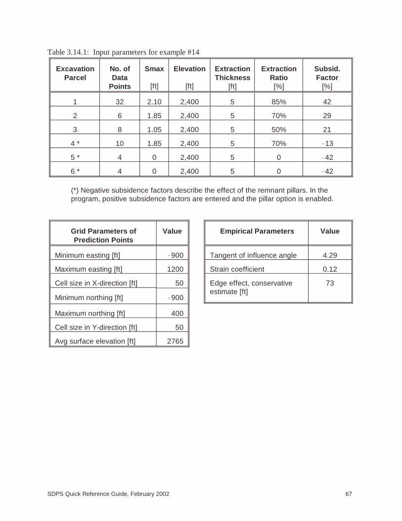
SDPS Quick Reference Guide, February 2002 67
ExcavationParcel
No. ofData
Points
Smax
[ft]
Elevation
[ft]
ExtractionThickness
[ft]
ExtractionRatio[%]
Subsid.Factor
[%]
1 32 2.10 2,400 5 85% 42
2 6 1.85 2,400 5 70% 29
3 8 1.05 2,400 5 50% 21
4 * 10 1.85 2,400 5 70% !13
5 * 4 0 2,400 5 0 !42
6 * 4 0 2,400 5 0 !42
(*) Negative subsidence factors describe the effect of the remnant pillars. In theprogram, positive subsidence factors are entered and the pillar option is enabled.
Grid Parameters ofPrediction Points
Value Empirical Parameters Value
Minimum easting [ft] !900 Tangent of influence angle 4.29
Maximum easting [ft] 1200 Strain coefficient 0.12
Cell size in X-direction [ft] 50 Edge effect, conservativeestimate [ft]
73
Minimum northing [ft] !900
Maximum northing [ft] 400
Cell size in Y-direction [ft] 50
Avg surface elevation [ft] 2765
Table 3.14.1: Input parameters for example #14

SDPS Quick Reference Guide, February 2002 68
[MINE PLAN DATA][Polygonal Mine Plan]Total Parcels: 6Parcel No: 1 -> Points: 32 Status: Active PanelPoint No Easting Northing Seam Extraction Subs.
Elevation Thickness Factor3.000 806.54 -258.31 2425.00 5.00 42.004.000 637.79 -159.98 2415.00 5.00 42.005.000 486.75 64.68 2405.00 5.00 42.006.000 487.98 163.35 2400.00 5.00 42.007.000 392.82 167.22 2400.00 5.00 42.008.000 391.41 139.84 2400.00 5.00 42.009.000 133.76 89.74 2390.00 5.00 42.0010.000 130.54 175.49 2390.00 5.00 42.0011.000 -286.65 183.04 2380.00 5.00 42.0012.000 -290.27 123.51 2380.00 5.00 42.0013.000 -360.26 120.56 2380.00 5.00 42.0014.000 -360.31 -89.85 2380.00 5.00 42.0015.000 -295.96 -92.80 2380.00 5.00 42.0016.000 -286.92 -650.15 2390.00 5.00 42.0017.000 -214.77 -653.62 2390.00 5.00 42.0018.000 -212.37 -692.75 2390.00 5.00 42.0019.000 -157.89 -653.75 2395.00 5.00 42.0020.000 -9.88 -654.90 2400.00 5.00 42.0021.000 -16.37 -588.94 2400.00 5.00 42.0022.000 134.34 -591.53 2410.00 5.00 42.0023.000 133.03 -537.35 2410.00 5.00 42.0024.000 63.49 -471.10 2410.00 5.00 42.0025.000 74.61 -178.74 2410.00 5.00 42.0026.000 212.24 -183.73 2410.00 5.00 42.0027.000 210.40 -45.24 2400.00 5.00 42.0028.000 238.25 -2.80 2400.00 5.00 42.0029.000 260.97 27.45 2400.00 5.00 42.0030.000 314.29 21.93 2400.00 5.00 42.0031.000 309.91 115.94 2395.00 5.00 42.0032.000 419.47 112.37 2400.00 5.00 42.0033.000 421.44 -229.67 2420.00 5.00 42.0034.000 778.03 -300.05 2430.00 5.00 42.00
Parcel No: 2 -> Points: 6 Status: Active PanelPoint No Easting Northing Seam Extraction Subs.
Elevation Thickness Factor35.000 417.98 -48.65 2405.00 5.00 29.0036.000 420.86 113.02 2400.00 5.00 29.0037.000 313.33 115.85 2395.00 5.00 29.0038.000 313.57 20.58 2400.00 5.00 29.0039.000 260.22 24.73 2400.00 5.00 29.0040.000 211.09 -45.26 2400.00 5.00 29.00
Table 3.14.2: Mine plan coordinates, example #14

SDPS Quick Reference Guide, February 2002 69
Parcel No: 3 -> Points: 8 Status: Active PanelPoint No Easting Northing Seam Extraction Subs.
Elevation Thickness Factor41.000 419.33 -231.67 2420.00 5.00 21.0042.000 417.94 -50.02 2405.00 5.00 21.0043.000 211.77 -45.28 2400.00 5.00 21.0044.000 213.59 -184.45 2410.00 5.00 21.0045.000 75.26 -180.13 2410.00 5.00 21.0046.000 68.56 -304.69 2410.00 5.00 21.0047.000 337.84 -306.98 2415.00 5.00 21.0048.000 338.21 -215.15 2415.00 5.00 21.00
Parcel No: 4 -> Points: 10 Status: Active PillarPoint No Easting Northing Seam Extraction Subs.
Elevation Thickness Factor49.000 -89.44 98.35 2390.00 5.00 -13.0050.000 -141.49 99.72 2390.00 5.00 -13.0051.000 -148.07 -540.92 2400.00 5.00 -13.0052.000 -209.83 -544.09 2400.00 5.00 -13.0053.000 -207.53 -638.73 2390.00 5.00 -13.0054.000 -105.39 -638.00 2395.00 5.00 -13.0055.000 -107.91 -421.35 2400.00 5.00 -13.0056.000 63.19 -404.61 2410.00 5.00 -13.0057.000 61.87 -376.48 2410.00 5.00 -13.0058.000 -110.74 -320.53 2400.00 5.00 -13.00
Parcel No: 5 -> Points: 4 Status: Active PillarPoint No Easting Northing Seam Extraction Subs.
Elevation Thickness Factor59.000 120.82 92.82 2390.00 5.00 -42.0060.000 74.95 94.71 2390.00 5.00 -42.0061.000 76.40 45.33 2390.00 5.00 -42.0062.000 126.43 45.38 2390.00 5.00 -42.00
Parcel No: 6 -> Points: 4 Status: Active PillarPoint No Easting Northing Seam Extraction Subs.
Elevation Thickness Factor63.000 189.84 32.75 2395.00 5.00 -42.0064.000 150.24 38.59 2395.00 5.00 -42.0065.000 143.12 -23.59 2395.00 5.00 -42.0066.000 191.66 -28.30 2395.00 5.00 -42.00
Table 3.14.3: Mine plan coordinates, continued, example #14

SDPS Quick Reference Guide, February 2002 70
Scattered PointsTransverse Profile
Point No Easting Northing Elevation186 575.02 -0.15 2834.26187 549.91 -0.26 2836.55188 525.11 -0.21 2835.44189 500.01 -0.16 2832.53190 475.31 -0.18 2829.46191 450.27 -0.12 2826.09192 424.20 -0.11 2822.94193 400.25 -0.02 2820.42194 375.08 -0.15 2819.67195 350.40 -0.19 2820.14196 325.24 1.13 2820.49197 300.30 -0.22 2820.76198 275.31 -0.05 2821.77199 250.31 -0.20 2823.22200 225.21 -0.26 2824.45201 200.21 -0.15 2824.18202 175.25 -0.28 2822.27203 150.21 -0.34 2819.70204 125.37 -0.22 2815.94205 100.15 -0.24 2811.96206 75.11 -0.17 2809.03207 50.10 -0.25 2805.59208 25.11 -0.27 2803.34209 -0.03 -0.13 2799.96210 -24.95 -0.15 2797.76211 -49.77 -0.29 2791.73212 -75.64 0.39 2787.67213 -99.67 0.02 2783.61214 -125.33 -0.31 2778.05215 -149.89 -0.08 2774.32216 -174.94 -0.18 2770.75217 -199.88 -0.16 2768.04218 -225.08 -0.17 2765.08219 -249.76 -0.07 2761.25220 -274.85 -0.15 2758.27221 -299.87 0.05 2754.71222 -324.94 -0.21 2750.46223 -349.87 -0.07 2746.48224 -374.80 -0.04 2741.49225 -399.93 -0.18 2735.62226 -424.20 -0.13 2733.80227 -449.97 0.11 2726.78228 -475.39 -0.13 2721.38229 -500.35 -0.02 2716.60230 -523.87 -0.89 2711.98231 -550.09 -5.46 2706.58232 -575.19 -6.01 2703.62233 -599.09 -5.77 2701.52
Scattered PointsLongitudinal Profile
Point No Easting Northing Elevation234 -0.15 600.43 2703.73235 -0.33 574.67 2709.03236 0.10 550.01 2713.94237 1.14 524.97 2715.99238 0.19 499.75 2720.67239 0.15 474.86 2724.51240 0.15 449.95 2728.80241 -0.61 424.80 2733.62242 0.31 399.67 2736.40243 -0.02 374.42 2738.85244 0.16 349.50 2741.92245 -0.03 323.58 2746.09246 -0.08 299.79 2747.68247 0.01 275.07 2750.19248 0.40 249.04 2754.17249 0.15 224.26 2758.77250 0.27 199.84 2767.18251 0.03 175.10 2770.00252 0.28 149.94 2770.86253 0.30 124.84 2770.91254 0.29 99.98 2775.58255 0.25 75.03 2784.12256 -0.04 49.86 2789.90257 0.36 26.41 2798.08258 -0.04 -0.13 2799.96259 0.20 -25.24 2802.69260 0.21 -45.09 2801.82261 0.07 -75.01 2802.35262 0.16 -99.65 2800.11263 -0.50 -124.95 2798.59264 0.22 -149.87 2795.08265 0.32 -175.09 2790.60266 0.25 -199.94 2784.78267 0.27 -224.97 2779.95268 0.36 -250.05 2774.73269 0.22 -275.50 2769.83270 0.56 -300.06 2765.09271 -0.85 -324.72 2758.94272 0.34 -350.12 2754.21273 0.49 -375.02 2758.21274 0.55 -399.95 2764.05275 0.25 -425.13 2771.88276 0.66 -450.22 2776.86277 0.49 -475.36 2780.58278 0.33 -500.18 2787.56279 -0.06 -525.02 2794.43280 0.46 -550.19 2797.32281 0.57 -575.08 2792.31282 0.43 -599.91 2784.80283 0.45 -625.22 2777.68284 0.51 -650.37 2769.98285 0.48 -675.02 2761.06286 0.57 -700.41 2749.46
Table 3.14.4: Prediction points coordinates, example #14

SDPS Quick Reference Guide, February 2002 71
Figure 3.14.2: Comparison of fitted and measured transverse subsidence profiles,example #14 (points 233-186)
Figure 3.14.3: Comparison of fitted and measured transverse strain profiles,example #14 (points 233-186)

SDPS Quick Reference Guide, February 2002 72
Figure 3.14.4: Comparison of fitted and measured longitudinal subsidenceprofiles, example #14 (points 286-234)
Figure 3.14.5: Comparison of fitted and measured longitudinal strain profiles,example #14 (points 286-234)

SDPS Quick Reference Guide, February 2002 73
Figure 3.14.6: Subsidence contours, example #14
Figure 3.14.7: Subsidence orthographic projection, example #14

SDPS Quick Reference Guide, February 2002 74
Figure 3.14.8: Maximum strain contours, example #14

SDPS Quick Reference Guide, February 2002 75
Figure 4.1.1: Pillar tributary area
Chapter 4: Pillar Stability AnalysisCalculationsPillar design should take into consideration the function of a pillar or a set of pillarduring the lifetime of a mining section. Since the original pillar design formulations wereproposed several decades ago, other formulations have been developed to addresspillar stability. The SDPS suite of programs, currently includes a traditional pillarstability program as well as the pillar stability formulations developed by the USBM(now NIOSH) regarding stability of pillars in longwall operations and stability of pillarsin room and pillar retreat operations.
4.1 Pillar Design for Room and PillarOperationsThe pillar stability program uses data that describe mine geometry and overburdencharacteristics, as well as coal pillar strength, to calculate safety factors based on fourwell-accepted pillar design formulations, namely those proposed by Bieniawski,Holland, Holland-Gaddy, and Obert & Duvall.
The safety factors associated with the aforementioned pillar equations can becalculated using the pillar tributary area concept (Figure 4.1.1). Parametric graphs for

SDPS Quick Reference Guide, February 2002 76
Figure 4.1.2: Protection area under a surface structure
the calculated safety factors can be generated for all formulations.
Also, the program can calculate the dimensions of the protection area (commonlyreferred to as “Pennsylvania Law”) a seam level underneath a surface structure.Extraction within this area should be limited if the surface structure is to be protected(Figure 4.1.2).
4.2 The ALPS MethodThe ALPS program is a stand alone program that was developed by NIOSH and isfreely distributed. It is included in the SDPS suite of programs to allow directcomparisons of pillar stability calculations. The program can calculate the ALPSstability factors, utilizing the widely accepted ALPS formulation for assessing pillarstability.
The ALPS method consists of three basic steps:• Estimating the loading that will be applied to the pillars during all the phases of
longwall mining;• Estimating the load-bearing capacity of the longwall pillar system, and;• Calculating stability factors (SF) by comparing the load to the load-bearing
capacity.
Since its development, the ALPS method has been verified by back-analysis of morethan 100 actual mining case histories (Mark, 1992). A complete discussion of theformulas used in ALPS can be found in that reference, copies of which are available

SDPS Quick Reference Guide, February 2002 77
from the author.
Recent research (Mark et al., 1994) has shown that the ALPS SF used in design shouldbe based on the structural competence of the mine roof, measured by the Coal MineRoof Rating (CMRR). A complete description of the CMRR, including field datacollection and procedures for calculating the ratings, have been provided by Molindaand Mark (1994). Spreadsheet programs for calculating the CMRR are also available(Riefenberg and Wuest, 1994).
Calculations are performed for two distinct modes:• the analysis mode (or forward model)• the sizing mode (or inverse model)
Analysis mode
The calculation phase of ALPS consists of several simple routines which compute thedevelopment loads, the abutment loads, the strengths and load-bearing capacities ofthe pillars, and the stability factors. The development loads, which are present beforelongwall mining, are determined by the depth of cover using the tributary area theory.Abutment loads occur as a portion of the weight of the overburden, that had beensupported by the excavated longwall panel, is transferred to the pillars. They aredetermined by the depth of cover, the panel width, and the abutment angle.
ALPS calculates the unit strength of the pillars using Bieniawski's empirical pillarstrength formula. The pillar strength is multiplied by load-bearing area and divided bythe crosscut spacing to compute the load-bearing capacity per foot of gate entry. Thenthe load-bearing capacity of the longwall pillar system is obtained by summing thecapacities of the individual pillars. Finally, stability factors are obtained by dividing thesystem's load- bearing capacity by the total loading.
In this mode, output consists of four (4) screens of data:• ALPS stability factors• Pillar load bearing capacity• Design loadings on pillar system (load per length of gate entry)• Individual pillar loading
The most important output provided by ALPS in the analysis mode are the stabilityfactors. These are determined for five loading conditions:
• Development loading: The loading on the pillar system before any longwallretreat mining. It is equal to the tributary area load.
• Headgate loading: The pillar loading adjacent to headgate corner of thelongwall face, which is equal to the development load plus the first frontabutment.
• Bleeder loading: The loading on a pillar system adjacent to a mined-out panel,which equals the development load plus the first side abutment.

SDPS Quick Reference Guide, February 2002 78
• Tailgate loading: The loading on a double-use gate entry system when it isadjacent to the tailgate corner of the longwall face, equal to the developmentload plus the first side abutment plus the second front abutment.
• Isolated loading: The loading on a pillar system located between two mined-outpanels, equal to the development load plus two side abutments.
Since most gate entry systems are used twice, first as a headgate and then as atailgate, the stability factor for tailgate loading is usually employed in design. That iswhy the results for tailgate loading are marked with asterisks (***) in the output. Single-use gate entries should be designed for either headgate or bleeder loading. As alreadyindicated, a Stability Factor between 0.7 and 1.3 is usually appropriate for gate entries,depending on the CMRR.
The pillar load bearing capacity screen includes the following:• pillar width,• width-to-height ratio,• the unit pillar strength calculated using the Bieniawski formula, and• the pillar load-bearing capacity per foot along the length of the gate entry.
The total pillar system load-bearing capacity, which is the sum of the load-bearingcapacities of the individual pillars, is the parameter that is needed to compute the SF.It is compared directly with design loadings that are also provided.
In the analysis mode, the last output screen provides estimates of the loadings appliedto the individual pillars in the gate entry system. The initial development loadings arecalculated using tributary area theory, and the subsequent abutment loadings areadded using the exponential stress decay formula developed in IC 9247, pp. 8-9. Asnoted in the output, the individual pillars loadings do not consider load transfer due topillar yielding. In general, if the applied stress exceeds a pillar's strength, load transfermay be assumed to occur. No estimates of individual pillar loads are provided for the"tailgate" and "isolated" loading phases, because the field data available from thosephases is not sufficient for the development of general formulas.
Sizing mode
In the sizing mode, ALPS will calculate the pillar size required to achieve desiredstability factors that are entered by the user. The user must choose a longwall pillarconfiguration from three options:
• a three-entry system employing equal-sized pillars;• a three-entry system employing a large "abutment" pillar and a small "yield"
pillar, (Yield-Abutment, YA), and;• a four-entry system employing a single large "abutment" pillar and two small
"yield" pillars (Yield-Abutment-Yield, YAY).
If either the "YA" or "YAY" options are chosen, ALPS requests the width of the "yield"

SDPS Quick Reference Guide, February 2002 79
pillar. In this case the actual pillar width, rather than the center-to-center entry spacing,is required.
ALPS also requires "stability factors" (SF) for the sizing mode. The suggested SFdepends on the CMRR for the case being analyzed, and ranges from approximately0.7 for strong roof (CMRR=75) to 1.3 for weak roof (CMRR=35).
In the sizing mode, ALPS computes the pillar widths that are necessary to achieve thedesired stability factors. A secant variation of Newton's root-solving algorithm is usedto solve the following equation, in which the pillar width is the only unknown:
0 = SF - (B/L)
In the equation SF is the stability factor, B is the pillar system load-bearing capacity,and L is the design loading. The algorithm terminates when successive iterations haveconverged on a pillar width to within 0.1 ft.
In this mode, output consists of four (4) screens of data:• ALPS pillar sizing results• Pillar load bearing capacity• Design loadings on pillar system (load per length of gate entry)• Individual pillar loading
In the sizing mode, ALPS prints the pillar widths which will provide the specified stabilityfactors for the specified design type. The pillar lengths are also given, because ALPSwill automatically increase the crosscut spacing to maintain square pillars if therequired pillar width exceeds the user-specified crosscut spacing. Also, as noted onthe printout, the pillar widths and lengths are actual dimensions, not centers.
The remaining 3 screens of output data are similar to those described above for theanalysis mode.
If the Coal Mine Roof Rating (CMRR) is known or can be estimated, the user simplyinputs the proper CMRR, and the program returns a suggested ALPS SF using theformula:
ALPS SF = 1.76 - 0.014 CMRR
According to Mark et al. (1994) this equation was derived from evaluations of tailgateperformance at more than 60 U.S. longwalls.
The CMRR library is a text file that contains summaries of roof descriptions and CMRRvalues obtained from 97 locations. The library helps users estimate the CMRR whendata is not available, and it allows users to check their own CMRR estimates againstobservations already made. More complete descriptions of the same 97 observationsmay be found in the appendix to Molinda and Mark, 1994.

SDPS Quick Reference Guide, February 2002 80
4.3 The ARMPS MethodThe ARMPS program is a stand alone program that was developed by NIOSH and isfreely distributed. It is included in the SDPS suite of programs to allow directcomparisons of pillar stability calculations. The program can calculate the ARMPSstability factors, utilizing the ARMPS formulation for assessing pillar stability.
Preventing pillar squeezes, massive pillar collapses, and bumps is critical to the safeand efficient retreat mining of coal. To help prevent these problems, the U.S. Bureau ofMines (now NIOSH) developed the Analysis of Retreat Mining Pillar Stability (ARMPS)computer program. ARMPS calculates Stability Factors (SF) based on estimates of theloads applied to, and the load bearing capacity of pillars during retreat miningoperations. The program can model the significant features of most retreat mininglayouts, including angled crosscuts, varied spacings between entries, barrier pillarsbetween the active section and old (side) gobs, and slab cuts in the barriers on retreat.It also features a pillar strength formula that considers the greater strength ofrectangular pillars. The program may be used to evaluate bleeder designs as well asactive workings.
A database of 160 pillar retreat case histories has been collected across the UnitedStates to verify the program. It was found that satisfactory conditions were very rarewhen the ARMPS SF was less than 0.75. Conversely, very few unsatisfactory designswere found where the ARMPS SF was greater than 1.5.
The loadings applied to the Active Mining Zone (AMZ) include development loads,abutment loads, and loads transferred from barrier pillars. The development loads,which are present before retreat mining, are determined by the depth of cover using the"tributary area" theory. Abutment loads occur as a result of retreat mining and gobformation. They are determined by the depth of cover, the width of the extraction front,the gob extents, and the abutment angles. The abutment loads are assumed to bedistributed following the abutment load distribution function. Only the portion of thefront abutment load that falls within the AMZ is included in the calculation of the SF.Loads are also applied to barrier pillars, but if the barriers are too small, there are threeways in which loads may be transferred to the AMZ:
• A portion of the side abutment load may be transferred according to theabutment load distribution function.
• If the barrier pillar yields, a portion of the side abutment load may be transferred,and;
• Front abutment loads may be transferred from yielded remnant barrier pillarsinby the pillar line.
Loadings that can occur in ARMPS are:
• Development: Loading Condition: 1, 2, 3, 4

SDPS Quick Reference Guide, February 2002 81
• Front Abutment: Loading Condition: 2, 3, 4• Side Abutments: Loading Condition: 3, 4
• Transfer From Remnant Barriers: Loading Condition: 3, 4
Stability factors are obtained by dividing the total load-bearing capacity of the AMZ bythe total load applied to it.
The next, critical step is the interpretation of the stability factor. The ARMPS methodhas been verified through back analysis of pillar recovery case histories. To date,more than 200 case histories have been obtained from 10 states, almost all from minevisits. They cover an extensive range of geologic conditions, roof rock cavabilitycharacteristics, extraction methods, depths of cover, and pillar geometries. Groundconditions in each case history have been categorized as being either satisfactory orunsatisfactory. Pillar failures responsible for unsatisfactory conditions included:
• Pillar squeezes;• Massive pillar collapses, usually accompanied by airblasts, and/or;• Coal pillar bumps.
Current research has begun to evaluate other factors that may contribute to satisfactoryconditions when the ARMPS SF falls between 0.75 and 1.5.

SDPS Quick Reference Guide, February 2002 82
Figure 4.3.1: Pillar geometry parameters
4.3 Example #15: Calculations Using thePillar Stability Analysis Module - Estimationof Pillar Safety Factors
Instructions1. Execute the Pillar Stability Analysis
Module.2. Select the Edit - Pillar Stability
option.3. Enter the following parameters (Fig-
ure 4.3.1):1. overburden depth = 500 ft
• pillar width = 40 ft• pillar length = 100 ft• pillar height = 6 ft• opening width = 20 ft• average extraction ratio = 45 %
(note that the tributary area ex-traction ratio is automatically
calculated and displayed in red)2. Click on the View Plan button to
see a plan view of the mine sectiondefined.
3. Click on the Pillar Strength tab ofthe current form (Figure 4.3.2).
4. Enter the value for pillar strength(e.g. 900 psi).
5. Click on the Output Options tab toselect the form of the output, i.e.either table or graph. In the case ofa graph output, the user can selectbetween four parametric graphs(Figure 4.3.3).
6. Click on Display Graph and a

SDPS Quick Reference Guide, February 2002 83
Figure 4.3.2: Pillar strength parameters
graph of all four pillar strength for-mulas will be plotted on the screen(Figure 4.3.4).
7. Close the viewing window.8. Click on the OK button to accept the
data.9. Select the File - Save menu item.
Notes for Advanced Users:1. Optionally the user can use the “Ad-
vanced Geometry” option and enterthe pillar geometry in terms of num-ber of entries, center-to-center dis-
tance between entries and center-to-center distance between cross-cuts. The results are similar but theextraction ratio is calculated as anaverage on all entries.
2. The range for the parametric graphsis based on a percentile maximumand minimum values as defined inthe Utilities-Options menu item.

SDPS Quick Reference Guide, February 2002 84
Figure 4.3.4: Parametric graph for four pillar strength formulas
Figure 4.3.3: Output options

SDPS Quick Reference Guide, February 2002 85
Figure 4.4.1: Structure and protection area geometry
4.4 Example #16: Calculations Using thePillar Stability Analysis Module - Estimationof Protection Area
Instructions1. Execute the Pillar Stability Analysis
Module.2. Select the Edit - Protection Area
option.3. Enter the following parameters (Fig-
ure 4.4.1):• overburden depth = 500 ft• structure width = 40 ft• structure length = 50 ft• keep the default values for the
remaining parameters4. Click on the Results button.5. The tabulated results will appear on
the screen (Figure 4.4.2).
Note:The extraction area is based on the as-sumed recovery, in this example, 50%.Using an appropriate seam thickness,this can be converted to extraction vol-ume and tonnages.

SDPS Quick Reference Guide, February 2002 86
Figure 4.4.2: Protection area results

SDPS Quick Reference Guide, February 2002 87
Figure 4.5.1: ALPS stability factors
4.5 Example #17: Calculations Using theALPS Module - Estimation of ALPS StabilityFactors
Instructions1. Execute the ALPS Module.2. Select the Input - Project Parame-
ters option.3. Enter the mine geometry parame-
ters as shown in Figure 4.5.1.4. Keep the default load parameters.5. Click on OK to exit the edit form.6. Select the Output - Stability Fac-
tors (Standard Geometry) menuoption.
7. The tabulated results will appear onthe screen (Figure 4.5.2).
8. Select the Output - Graph (ALPS
Classic) menu option.9. Select the SF vs Entry Height op-
tion. The graph shown in Figure4.5.3 will be created.
10. Close the forms and save the pro-ject.
Notes:• The “Advanced” tab in Figure 4.5.1
allows for entering slanted crosscutentries (Figure 4.5.4).

SDPS Quick Reference Guide, February 2002 88
Figure 4.5.2: ALPS results
Figure 4.5.3: Parametric graph for ALPS stability factors

SDPS Quick Reference Guide, February 2002 89
Figure 4.5.4: ALPS: Advanced geometry

SDPS Quick Reference Guide, February 2002 90
Figure 4.6.1: ARMPS input parameters
4.6 Example #18: Calculations Using theARMPS Module - Estimation of ARMPSStability Factors
Instructions1. Execute the ARMPS Module.2. Select the Input - Project Parame-
ters option.3. Enter the mine geometry parame-
ters as shown in Figure 4.6.1. Clickon View to plot the mine plan on thescreen (Figure 4.6.2).
4. Keep the default load parameters.5. Click on OK to exit the edit form.6. Select the Output - Stability Fac-
tors menu option.7. The tabulated results will appear on
the screen (Figure 4.6.3).8. Select the Output - Graph menu
option.9. Select the SF vs Entry Height op-
tion. The graph shown in Figure4.6.4 will be created.
10. Close the forms and save the pro-ject.
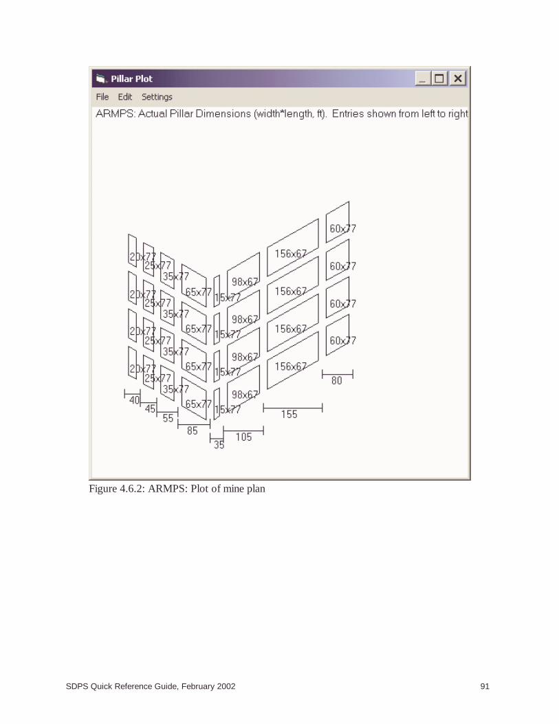
SDPS Quick Reference Guide, February 2002 91
Figure 4.6.2: ARMPS: Plot of mine plan
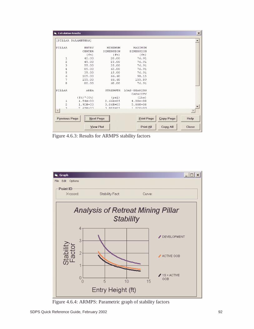
SDPS Quick Reference Guide, February 2002 92
Figure 4.6.4: ARMPS: Parametric graph of stability factors
Figure 4.6.3: Results for ARMPS stability factors

SDPS Quick Reference Guide, February 2002 93
Chapter 5: The Graphing ModuleThis SPDS module can create two- and three-dimensional images of the calculateddeformation indices and either display them on the screen or print them to a Windowsdevice. The main source of input to this program are files created by the solutionmodules of the influence function method.
The program can handle two types of files:• grid files (SDPS grid, Surfer grid and SurvCADD grid files)• XYZ files
The points represented by a grid file are the points defined at the cross-section ofhorizontal and vertical grid lines within the grid boundaries. Thus, grid files contain thefollowing information:• the minimum and maximum extent in the x-direction• the minimum and maximum extent in the y-direction• the step size in the x- and y-directions• the number of grid lines in the x- and y-directions• the value for the z-parameter, i.e. values for a particular deformation index, the
elevation, etc. for all points defined by the grid.
Notes:Grid files do not contain the x- and y-coordinates for each point, since these values canbe generated based on the above data.
5.1 Two-Dimensional Images: Cross-sectional plotsCross-sectional plots generated from grid files can be defined along any (horizontal orvertical) grid line at any intercept. Depending on the orientation of the cross-section,the x-axis of the graph will represent either the x- or the y-axis of the grid. The y-axis ofthe graph will always be the z-parameter for the corresponding points. The user has theoption to view cross-sections created at different intercept values either on the x- or y-direction.
When data are available in an XYZ file, which may or may not be defined on a regulargrid, the program can only create one cross-sectional plot, which is termed a directionalcross-section. This plot includes all points in the file taken in the sequence read fromthe file, i.e. from first to last. The file specified for the profile should only contain eithertwo or three columns of data. If the file contains two columns of data, then the programassumes that the first is the x- and the second is the y-coordinate of the points to beplotted on the cross-sectional plot. These points are plotted directly without anyscaling. If the file contains three columns of data, then the program assumes that it is

SDPS Quick Reference Guide, February 2002 94
an XYZ file. In this case the user has three options:
• to use an X-projection (i.e. use the x- and z-columns)• to use a Y-projection (i.e. use the y- and z-columns)• to use an Axial projection, in which case the origin of the x-axis is set to zero (0)
and the distance between the points is the actual horizontal (radial) distance.
5.2 Two-Dimensional Images: Vector plotsVector plot can be created only for those indices where a direction of a horizontalvector representing this index is available. For example vector plots can be plotted forthe horizontal displacements, for the principal horizontal strains, for the principalhorizontal curvatures as well as for the slopes.
5.3 Three-Dimensional ImagesThe program can also create three-dimensional graphs. These graphs can only begenerated if deformation have been calculated on a grid. External gridding packages(such as Surfer or SurvCADD) can be used to grid the prediction points, prior tocalculations.
Notes:The graphing module can not directly load individual files for plotting. Files are loadedindirectly utilizing project information generated by the Influence Function Method.

SDPS Quick Reference Guide, February 2002 95
Chapter 6: ReferencesSubsidence References
Karmis, M., A. Jarosz, P. Schilizzi and Z. Agioutantis, "Surface DeformationCharacteristics above Undermined Areas: Experiences from the Eastern UnitedStates", Civil Engineering Transactions, Vol, CE29, no 2, The Institution of Engineers,Australia, April, 1987, pp. 106-114.
Karmis, M., A. Jarosz and Z. Agioutantis, "An Integrated Surface Movement MonitoringSystem for Undermined Areas", Proceedings, VII International Congress on MineSurveying, Volume X, Leningrad, USSR, June 28-July 2, 1988, pp. 42-48.
Agioutantis, Z. and M. Karmis, "Developing Improved Methods of Predicting SurfaceDisplacements due to Underground Mining Through the Integration of Empirical Indicesinto Numerical Modeling", Mining Science and Geotechnology, 7, 1988, pp. 133-148.
Agioutantis, Z., M. Karmis and A. Jarosz, "Prediction of Surface Subsidence and Strainin the Appalachian Coalfields Using Numerical Methods", Proceedings, 7th Conferenceon Ground Control in Mining, West Virginia University, Morgantown, West Virginia,August 3-5, 1988, pp. 95-100.
Hustrulid, W. A., 1996, A review of Coal Pillar Strength Formulas; Rock Mechanics 8,115-145, Springer-Verlag 1976.
Karmis M., A. Jarosz, and Z. Agioutantis, "Predicting Subsidence with a Computer",Coal, vol 26, no. 12, December, 1989, pp. 54-61.
Karmis, M., Z. Agioutantis and A. Jarosz, "Recent Developments in the Application ofthe Influence Function Method for Ground Movement Predictions in the U.S.", MiningScience and Geotechnology, 1990, Vol. 10, pp. 233-245.
Karmis, M., Z. Agioutantis and A. Jarosz, "Subsidence Prediction Techniques in theUnited States: A State-of-the-Art Review", Mineral Resources Engineering, 1990, Vol.3, No 3, pp. 197-210.
Karmis, M., C. Haycocks and Z. Agioutantis, "The Prediction of Ground MovementsCaused by Mining", Proceedings, 3rd Subsidence Workshop Due to UndergroundMining, Morgantown, West Virginia, June 1-4, 1992, pp. 1-9.
Karmis, M., J. Mastoris, and Z. Agioutantis, "Potential of the 'Damage Angle' Conceptfor Assessing Surface Impacts of Underground Mining", Transactions, Society forMining, Metallurgy and Exploration, Inc., 1994, Vol. 296, pp. 1883-1886.
VPI&SU, (1987), "Prediction of Ground Movements Due to Underground Mining in the

SDPS Quick Reference Guide, February 2002 96
Eastern United States Coalfields", Final Report, Office of Surface Mining, Reclamationand Enforcement, U.S. Department of Interior, Grant No. J5140137, Volume I, 205p.,Volume II, 112p.
Pillar Design References
Bieniawski, Z.T., (1992), "A Method Revisited: Coal Pillar Strength Formula Based onField Investigations", Proceedings, Workshop on Coal Pillar Mechanics and Design,USBM IC 9315, 1992, pp. 158-165.
Mark, C., (1990), "Pillar Design Methods for Longwall Mining", USBM IC 9247, 53p.
Peng, S.S., (1986), Coal Mine Ground Control, 2nd edition, John Wiley & Sons, NewYork, pp. 237-264.
ALPS References
Carr, F. and E. Martin, (1986), "Development of Pillar Design Alternatives for theControl of Abutment Stresses During Retreat Longwall Mining in Deep Coal Mines",Proceedings, AMC Coal Convention, American Mining Congress, Coal MiningTechnology, Economics, and Policy, 14 pp.
Carr, F. and A. H. Wilson, (1982), "A New Approach to the Design of Multi-EntryDevelopments for Retreat Longwall Mining", Proceedings, 2nd Conference on GroundControl in Mining, WV University, Morgantown, WV, 1982, pp. 1-21.
Choi, D.S. and D.L. McCain, (1980), "Design of Longwall Pillar Systems", Transactions,Society for Mining, Metallurgy and Exploration, AIME, v. 268, pp. 1761-1764.
Hsuing, S.M. and S.S. Peng, "Chain Pillar Design for U.S. Longwall Panels", MiningScience and Technology, v.2, pp. 279-305.
Mark, C., (1992), "Analysis of Longwall Pillar Stability (ALPS)--An Update",Proceedings, Workshop on Coal Pillar Mechanics and Design, USBM IC 9315, pp. 238-249.
Mark, C., F.E. Chase, and G.M. Molinda, (1994), "Design of Longwall Gate EntrySystems Using Roof Classification", Proceedings, New Technology for LongwallGround Control, USBM SP 94-01, pp. 5-17.
Molinda, G.M. and C. Mark, (1994), "The Coal Mine Roof Rating (CMRR): A PracticalGuide for Rock Mass Classification in Coal Mines", USBM IC 9387, 83 pp.
Riefenberg, J. and W. J. Wuest (1994), "A Personal Computer Program andSpreadsheet for Calculating the Coal Mine Roof Rating (CMRR)", USBM IC 9386, 39p.

SDPS Quick Reference Guide, February 2002 97
ARMPS References
Chase, F. E., R. K. Zipf, and C. Mark (1994), The Massive Collapse of Coal Pillars -Case Histories from the United States, Proceedings of the 13th Conference on GroundControl in Mining, pp. 69-80.
Mark, C., F. E. Chase, and A. Campoli (1995), Analysis of Retreat Mining PillarStability, Proceedings of the 14th International Conference on Ground Control inMining, Morgantown, WV, pp. 63-71.
Mark, C. and T. M. Barton (1996), The Uniaxial Compressive Strength of Coal: Shouldit be Used to Design Pillars?, Proceedings, 15th International Conference on GroundControl, Golden, CO., 18 p.
Mark, C. Pillar Design Methods for Longwall Mining (1990), USBM IC 9247, 53 p.
Mark, C. and A. T. Iannacchione (1992), Coal Pillar Mechanics: Theoretical Modelsand Field Measurements Compared. Paper in the Proceedings of the Workshop onCoal Pillar Mechanics and Design, USBM IC 9315, Santa Fe, NM, pp.78-93.

SDPS Quick Reference Guide, February 2002 98
Appendix 1: Program ReferenceThis section includes a detailed reference for the menu options for each programmodule.

SDPS Quick Reference Guide, February 2002 99
A1.1 The Profile Function ModuleA1.1.1 The File MenuUse the File menu option to access various file management operations such as:1. Create New Files
• Use the New option to erase the existing dataset (if any) from memoryand create a new (blank) dataset. All related entries are set to their initialvalues. Note that the program will prompt you whether to save the currentfile to disk.
2. Open Existing Files• Use the Open option to load a file (dataset) from the disk into program
memory. To use Open:i. Select the Open option from the File menu. The program displays
a listing of the available files in the current data directory.ii. Optionally, select a different drive or directory using the mouse or
the cursor control keys.iii. Select or enter a filename.
• Notes:i. If the file extension is omitted, the default extension will be
appended.ii. If the current dataset is not saved, the program will prompt whether
to save changes or not before discarding the current dataset.3. Save Files
• Use the Save option to save an existing file (dataset) to the drive ordirectory from which it was originally loaded. Any changes that weremade, since the last time the file was saved, will be saved on the disk.The filename stays the same and the file remains in memory. To useSave:i. Select the Save option from the File menu.
• Notes:i. If the file has never been saved using the Save As option,
choosing Save automatically displays the Save As dialogue box,which prompts for a filename before saving it.
4. Save Files under Different Names (Save As)• Use the Save As option to save a file and give it a new name. To use
Save As:i. Select the Save As option from the File menu. The program
displays a listing of the available files in the current data directory.ii. Optionally, select a different drive or directory.iii. Select or enter a filename.
• Notes:i. If the file exists, the program will prompt whether to overwrite the
existing file.ii. Use Save for a faster save operation.
5. Print Files• Use the Print option to print the current dataset (file) from program

SDPS Quick Reference Guide, February 2002 100
memory to the printer.• Notes:
i. This operation does not send any control characters to the printer.All output is ASCII text. All printed text will appear in the defaultprinter font.
ii. The default values for paper margins are:left margin = 1 inchtop margin = 1 inchbottom margin = 1 inch
6. Browse Text Files• Use the Browse option to view a text (ASCII) file in a specified directory.
Both an internal or an external browser can be used to browse such files.No editing is allowed during browsing using the internal browser.
• Use the pattern field to specify a file pattern (i.e. *.txt). The file window willbe reset to conform to the specified pattern. The default pattern is *.*.
• More than one patterns can be applied using “;” as delimiter (e.g.*.txt;*.dxf).
• Use the Set Font command button to specify the type and size of font forthe displayed text in the internal browser. These settings are saved in themodule.INI file.
• Use the cursor control keys to move within the browse window.• If an external ASCII viewer is used (i.e. NOTEPAD.EXE) as specified in
the Utilities-Settings form, then the maximum file size to browse is set bythe limits of the external browser.
• Notes:i. The internal browser has a limit of approximately 25000 characters.
7. Exit the Program• Use the Exit option when ready to exit this program and return to the
original environment. The program will prompt you to save the current fileto disk, if not already saved.
A1.1.2 The Edit MenuUse the Edit menu option to access various data input, data editing operations anddata graphing operations such as:1. Project Description
• This is an arbitrary 300 character description of the model beinggenerated. It is a good idea to make this a fairly detailed description ofthe specifics of the input file. This text may be a single line of charactersor may contain "carriage return characters".
• The user can also set the type of units that will be used in the currentproject. The program is designed to use two different sets of units: ft andm.
2. Profile Function Input Parameters• The profile function method uses data that describe mine geometry and
overburden characteristics to generate a profile of surface subsidencedue to underground mining. The formulation assumes uniform excavationconditions and calculates subsidence for each half-panel. The following

SDPS Quick Reference Guide, February 2002 101
parameters are necessary for the calculations:i. Subsidence Parameter Data: which includes:
(1) The mining system: A longwall or a room-and-pillar miningsystem can be selected. If a longwall system is selected, theextraction ratio input field is disabled and the extraction ratiois internally assumed 100%.
(2) The panel width: The least panel dimension should bespecified as panel width.
(3) The panel depth (depth of cover or overburden depth): Thedepth of cover to the top of the seam should be specified.
(4) The extraction thickness (seam height, mining height): Theterm extraction thickness reflects the total thickness mined,not just the seam thickness.
(5) The extraction ratio: This parameter can only be specifiedfor room-and-pillar panels. The lower limit currentlyaccepted is 75%.
(6) The percent hardrock in the overburden (%HR): Thisparameter can be determined by calculating the % ofcompetent strata in the overburden (i.e. limestone,sandstone beds, etc.)
(7) The surface point spacing: This parameter is used to definethe spacing of the surface points for calculating thesubsidence profile. The points are assumed on a transverseline starting from the panel center.
(8) The prediction mode: This parameter specifies the type ofprediction equation to be used. The conservative equationgives an envelop line, while the average equation gives aprediction which is based on the statistical average of thedatabase.
(9) The definition of zero subsidence: These parameters areused to define the point to be considered as point of zerosubsidence. This can be defined either as a percentage ofthe maximum subsidence value or as a fixed value (ft or m).The angle of draw may be calculated based on thesevalues.
ii. Output Options: These options include:(1) Results mode: This option allows the user to select whether
to the results in the form of graph (Display Graph) or in theform of a table (Display Table). The default "results mode"may be set through the Profile Function Program Options.
(2) Graph mode: This option is enabled only when the DisplayGraph option is selected and allows the user to selectwhether the graph will display only one curve at a time(Single Curve) or the graph engine will allow overlaying ofprofiles (Append Curve) up to the maximum numberspecified in the graph options form. The default "graph

SDPS Quick Reference Guide, February 2002 102
mode" may be set through the Profile Function ProgramOptions.
(3) Show Angles from the Rib: This option is enabled only whenthe Display Table option is selected and allows the user toselect whether the angles from the rib to each surface pointon the surface will be calculated. This is an indirect way tocalculate the angle of draw, where the user makes thechoice of the cutoff (zero subsidence) point.
(4) Plot Angles of Draw: This option is enabled only when theDisplay Graph option is selected and allows the user toselect whether the angle of draw corresponding to eachcurve will be plotted on the graph. Note that this option isautomatically disabled when one or more curves are plottedon the screen. In other words, the user can not select ordeselect this option in the middle of a graphing session. Toenable the option, either clear the current graph or close thegraph window and recreate the last graph.
3. Basic Graph Formatting Options (applies to more than one modules)• The user can set the basic graph formatting parameters such as:
i. The graph title: The graph title is a text string placed over thegraph.
ii. The graph x-axis title: The x-axis title is a text string placed belowthe x-axis of the graph.
iii. The graph y-axis title: The y-axis title is a text string placed to theleft of the y-axis of the graph.
iv. The grid style: Four grid styles are available: Horizontal lines,vertical lines, horizontal and vertical lines, no grid lines.
v. The graph style: Three graph styles are available: lines, symbols,lines and symbols.
vi. The maximum number of curves: The user can specify themaximum number of curves that can be overlaid on the graph.When this number is exceeded (in the Append Curve mode) theprogram will instruct the user to clear the graph before proceeding.
vii. The curve legend: This option enables or disables the legend boxin the graph. When this options is enabled, The combination of ascroll box and a text box allows the user to modify the defaultlegend titles for all graphs on the screen.
viii. Symbol size: With this scroll box the user can set the size of thesymbols used by the graph object. The scroll box is enabled onlyfor a graph type of "symbols" or "lines and symbols".
ix. Default parameter options: There are two default parameteroptions: a) to set the default parameters (i.e. graph title, x-axis title,etc.) every time the graph options form is invoked, and b) to set theformat parameters to used in the previous graphing session. Thesevalues are saved in the corresponding module.INI file.
4. The Graph Form (applies to more than one modules)

SDPS Quick Reference Guide, February 2002 103
• This form is used to display a graph generated by the calling program.The menu options available are:i. [File Import]: This option imports data to the graph from a space or
tab delimited file. This option is not available in all modules.ii. [File Export]: This option saves the data in the graph in a space or
tab delimited file. This option is not available in all modules.iii. [File-Save]: This option saves the graph as an image file. The
image file is in WMF format (Windows Metafile). This option is notavailable in all modules.
iv. File-Print: This option prints the graph to the default printer.v. File-Exit: This option clears the graph and closes the graph form.vi. [File-Exit and Keep]: This option hides the graph form. The form is
shown again when the graphing routines are called. Graphs arepreserved between calls. This option is not available in allmodules.
vii. Edit-Copy: This option copies the current graph object to theclipboard for use in other applications.
viii. [Edit-Clear]: This option clears the graph and allows plotting ofmore curves. This option is not available in all modules. Note thatalthough the graph is cleared from the screen, the graphparameters are kept internally. A number of options, such asenabling or disabling the graph tool bar or invoking the optionsform, will restore the graph to the screen.
ix. Options-Graph Toolbar: This option enables the graph tool bar.Using the graph toolbar the user has more choices regarding theappearance of the graph than those provided by the basic graphformatting options. The options in the graph toolbar have their ownon-line help file. This option is disabled by default.
x. Options-Point ID: This allows the user to click on a point a curve onthe graph and the coordinates of this point will be displayed in theappropriate boxes.
xi. Options-Basic Options: This option loads the graph options formwhich includes basic graph formatting options.
• Notes:i. Command buttons available on some forms are specific to each
module and are usually self explanatory.ii. Graphics support is provided by Graphics Server 4.53, which is an
independent graph control not included in the Microsoft VisualBasic 4.0 package.
A1.1.3 The Utilities MenuUse the Utilities menu option to access various program options such as:1. Settings (applies to more than one modules)
• This form is used to define a number of default parameters and settingsfor the program:i. Default Units: This setting controls the default units' selection used
when the program is executed. This setting is also used as an

SDPS Quick Reference Guide, February 2002 104
initial value in the Project Description form. This setting is saved inthe module.INI file.
ii. Default File Extension for Input Files: This setting is the default 3-letter extension used in the Open and Save dialog boxes in the FileMenu. This setting is saved in the module.INI file.
iii. Data Path: This setting is the default path used in the Open andSave dialog boxes in the File Menu. This setting is saved in themodule.INI file.
iv. Display Command History Window: This parameter controlswhether the program will display recently executed commands (andtheir resulting actions). This setting is saved in the module.INI file.
v. Maximum Characters in Command History Window: Maximumnumber of characters displayed in the command history window,before it is cleared. This setting is enabled only if the DisplayCommand History Window option is enabled. This setting is savedin the module.INI file.
vi. Font Type and Size in Command History Window: This button setsthe type and size of font used in the command history window. Thissetting is enabled only if the Display Command History Windowoption is enabled. This setting is saved in the module.INI file.
vii. Keep Recently Accessed File Names: This parameter controlswhether the program will keep up to four (4) recently accesseddata files (opened or saved) as menu items in the File Menu. Thissetting is saved in the module.INI file.
viii. Show Disclaimer: This parameter controls whether the disclaimermessage will be displayed when loading the program. This settingis saved in the module.INI file.
ix. Maximize Main Menu Window: This parameter controls whether themain menu window will be maximized when loading the program.This setting is saved in the module.INI file.
x. Enable Toolbar: This parameter controls whether the main menutoolbar will be enabled when viewing the main menu. This settingis saved in the module.INI file.
xi. External Viewer: The user can set the application name of anexternal ASCII viewer for viewing reports and other ASCII filesgenerated by the program. The default viewer in NOTEPAD.EXEsupplied with the windows operating system. Note that prior toWindows2000, NOTEPAD.EXE could only edit / display files up to64K. This setting is saved in the module.INI file.
2. Options• This form is used to define a number of default parameters and options
pertaining specifically to the Profile Function Method Module. Theseoptions include:i. General
(1) Load Input Screen on File Open: This option will load themain parameter input screen when the user selects File -

SDPS Quick Reference Guide, February 2002 105
Open (filename) or File - New.(2) Print Module Version Information: This option will enable
printing of a module header when a print function isexecuted.
(3) Warn User When Input Data Outside Usual Range: Whenthis option is enabled, then warning messages will be issuedif input data are outside usual range. This option does notaffect data that exceed absolute limits.
ii. Default Settings(1) Show Angles from the Rib: This option will set the default
option for displaying (or not) angles from the rib whenresults are shown in table form.
(2) Plot Angles of Draw: This option will set the default optionfor ploting an angle of draw when graphing the calculatedprofile.
(3) Default Results Mode: This option will set the default resultsmode in the main parameter input screen (display graph ordisplay table)
(4) Default Graph Mode: This option will set the default graphmode in the main parameter input screen (append curve orsingle curve)
3. Unit Conversions (applies to more than one modules)• This utility can be used to convert between English and metric units for 4
types of units:i. Length: Conversion between feet, inches, meters and centimeters
is supported.ii. Pressure: Conversion between psi (pounds per square inch), Pa
(Pascals) and MPa (MegaPascals) is supported.iii. Stress (Pressure) Gradient: Conversion between psi/ft (psi per
foot), psi/in (psi per inch), MPa/m (MegaPascal per meter) andPa/m (Pascal per meter) is supported.
iv. Load Gradient: Conversion between lbs/ft (pounds per foot), lbs/in(pounds per inch), kN/m (kiloNewton per meter) and MN/m(MegaNewton per meter) is supported.
• Notes:1 Pa = 1 Newton per square meter1 psi = 1 pound per square inch
4. Clear History Window (applies to more than one modules)• This option clears the history (activity) window.
5. Close/Restore History Window (applies to more than one modules)• This option closes or restores the history (activity) window according to
the current window status.6. Copy History Window (applies to more than one modules)
• This option copies the contents of the history window to the clipboard.You can then paste them to any text handling program for furtherprocessing.

SDPS Quick Reference Guide, February 2002 106
A1.2 The Influence Function ModuleA1.2.1 The File MenuUse the File menu option to access various file management operations such as:1. Create New Files
• This function has three options:i. Create New Project Filesii. Create New Mine Plan Filesiii. Create New Prediction Point Files
• Use the New option to load a blank dataset into program memory.• Creating a new project loads resets the default values for the type of mine
plan, prediction points, units and overburden information.• Creating a new mine plan, resets the default values for the mine plan.
Similarly, creating a new set of prediction points, resets the defaultsvalues for the set. To use New:i. Select the New option from the File menu.
2. Open Existing Files• This function has three options:
i. Open Project Filesii. Open Mine Plan Filesiii. Open Prediction Point Files
• Use the open option to load a file (dataset) from the disk into programmemory.
• Opening a project loads saves the mine plan, prediction point andoverburden information from a single file. Opening a mine plan loads justthe mine plan geometry from a file. Similarly, opening the predictionpoints, opens just the prediction point geometry from a file. These last twofeatures are very useful when creating sets of project files based onsimilar mine plans, but with different surface topography, or when usingthe same surface topography to create project files with different mineplans. To use Open:i. Select the Open option from the File menu. The program displays
a listing of the available files in the current data directory.ii. Optionally, select a different drive or directory using the mouse or
the cursor control keys.iii. Select or enter a filename.
• Notes:i. If the file extension is omitted, the default extension will be
appended.ii. If the current dataset is not saved, the program will prompt whether
to save changes or not before discarding the current dataset.3. Save Files
• This function has three options:i. Save Project Filesii. Save Mine Plan Filesiii. Save Prediction Point Files

SDPS Quick Reference Guide, February 2002 107
• Use the Save option to save an existing file (dataset) to the drive ordirectory from which it was originally loaded. Any changes that weremade, since the last time the file was saved, will be saved on the disk.The filename stays the same and the file remains in memory.
• Use the Save As option to save an existing file (dataset) under a newfilename specification.
• Saving a project saves the mine plan, prediction point and overburdeninformation in a single file. Saving a mine plan saves just the mine plangeometry in a file. Similarly, saving the prediction points, saves just theprediction point geometry in a file. These last two features are very usefulwhen creating sets of project files based on similar mine plans but withdifferent surface topography, or when using the same surface topographyto create project files with different mine plans. To use Save:i. Select the Save option from the File menu.
• To use Save As:i. Select the Save As option from the File menu.
• Notes:i. If the file has never been saved using the Save As option,
choosing Save automatically displays the Save As dialogue box,which prompts for a filename before saving it.
4. Import Data• Use the File - Import option to import either an SDPS project created by
SDPS version 4.x software or import SDPS components (i.e. mine plansand sets of prediction points) from other sources, mainly AutoCAD files.The import form (for SDPS components) has the following options:
• Import a mine plan from an AutoCAD DXF file. The user should specifythe following:i. The layer names of active and hidden (not-active) entities. Default
layer names are PANELS for extraction panels and PILLARS forpillars.
ii. The type of the extracted area (longwall, high extraction room-and-pillar or low extraction room-and-pillar).
iii. Whether to import elevations from the AutoCAD file or to use anaverage elevation as specified in the import form.
iv. The subsidence parameters (subsidence factor or percenthardrock) associated with every point in each imported parcel.
v. Whether to apply a scale factor to the coordinates imported fromthe AutoCAD file.
vi. The thickness for every point in each imported parcel.vii. Whether to append the data to the existing set or start a new set.
• Notes: Importing will always result in a polygonal mine plan.• Import prediction points from an AutoCAD DXF file. The user should
specify the following:i. The layer names of active and hidden (not-active) entities. The
default layer name is POINTS.ii. Whether to import elevations from the AutoCAD file or to use an

SDPS Quick Reference Guide, February 2002 108
average elevation as specified in the import form.iii. Whether to apply a scale factor to the coordinates imported from
the AutoCAD file.iv. Whether to append the data to the existing set or start a new set.
• Import prediction points from an XYZ (ASCII) file: The XYZ points optionwill import an XYZ ASCII data file as a scattered surface point set. Thedata can be either space-delimited or comma-delimited. The program willpreview the data file and try to determine the number of header (textlines), if any, as well as the number of columns in the data set.
• Import a set of prediction points from a Surfer grid file (ASCII). The gridfrom surfer option will import a grid of surface points. The Surfer grid fileshould be in a DOS format and saved in ASCII. No options are neededfor this function. All information will be retrieved from the grid file header.
• Import a set of prediction points from a SurvCADD grid file. The grid fromSurvCADD option will import a grid of surface points. No options areneeded for this function. All information will be retrieved from the grid fileheader.
• Import points and/or panels and/or pillars directly from AutoCAD 2000DWG files. This selection invokes a new form with the following options:i. Import points from contours. The user should specify the following:
(1) The file name of the AutoCAD file (DWG file) that holds thedata. The program will read the file and import the layernames.
(2) The layer names of the CONTOURS as they can beselected from the combo box.
(3) The entity type for the contour lines. Here only two optionsare supported: LWPOLYLINE and 3DPOLYLINE.
(4) Whether to append the data to the existing set or start anew set.
ii. Import mine plan. The user should specify the following:(1) The file name of the AutoCAD file (DWG file) that holds the
data. The program will read the file and import the layernames.
(2) The layer names of the PANELS and the PILLARS as theycan be selected from the combo boxes.
(3) The entity type for the contour lines. Here only two optionsare supported: LWPOLYLINE and 3DPOLYLINE.
(4) The subsidence factor associated with every point in eachimported parcel.
(5) The thickness for every point in each imported parcel.(6) Whether to append the data to the existing set or start a
new set.iii. Notes:
(1) The routine for reading directly from AutoCAD 2000 wasoriginally designed by Steven J. Schafrik.
(2) If all input data is digitized to a single AutoCAD file (in

SDPS Quick Reference Guide, February 2002 109
different layers) then the whole project can be imported intwo steps. One step for the mine plan and one step for theprediction points.
(3) Surface topography contour lines can be imported asprediction points only through direct interaction withAutoCAD 2000.
(4) When importing data in a new project, the program willautomatically switch the mine plan type and/or the predictionpoint type to one needed for the import. If, however, dataare imported into an existing project, this process will haveto be done manually by the user.
5. Export Data• Use the File - Export option to export either a whole SDPS project to
AutoCAD DXF format or to export SDPS components to XYZ format. Theexport form has three options:i. Export the current project to AutoCAD DXF formatii. Export the current mine plan to XYZ point formatiii. Export the current surface points to XYZ point format
• In the case of AutoCAD output, the program will create a DXF file with themine geometry information as well as the surface topography data savedin separate layers. Note that subsidence information as well as point idinformation is lost during this process.
• In the case of XYZ output all data is converted to XYZ coordinates andstored to files. Additional information such as point ids and subsidencedata are preserved.
6. Print Files• Use the Print option to print an existing file (dataset) to any windows
printer. This function prints the data as its currently in the computermemory. This function has three optionsi. Print Project Filesii. Print Mine Plan Filesiii. Print Prediction Point Files
• To use Print: Select the Print option from the File menu.• Notes:
i. The file prints in the default printer font with a left margin of 1 inchand a top margin of 1 inch.
7. Browse Text Files• Use the Browse option to view a text (ASCII) file in a specified directory.
No editing is allowed during browsing.• Use the pattern field to specify a file pattern (i.e. *.txt). The file window will
be reset to conform to the specified pattern. The default pattern is *.*.• More than one patterns can be applied using “;” as delimiter (e.g.
*.txt;*.dxf).• Use the Set Font command button to specify the type and size of font for
the displayed text. These settings are saved in the module.INI file.

SDPS Quick Reference Guide, February 2002 110
• Use the cursor control keys to move within the browse window.• Notes:
i. The browser has a limit of approximately 25000 characters.8. Exit the Program
• Use the Exit option when ready to exit this program and return to theoriginal environment. The program will prompt you to save the current fileto disk, if not already saved.
A1.2.2 The Edit MenuThe influence function formulation supports several different types of excavationgeometry and prediction point layouts. Data that describe excavation geometry arereferred to as mine plan data, while data that describe the points on the surface (or anyother elevation), where deformation indices will be calculated, are referred to asprediction point data. Mine plan data can be specified as• a sequence of closed polygonal lines (polygonal mine plans)• rectangular entities parallel to the coordinate system (rectangular mine plans)Prediction point data can be represented by:• scattered points• points on a grid oriented parallel to the coordinate systemUse the Edit menu option to access various data input, data editing operations anddata graphing operations such as:1. Project Description:
• This is an arbitrary 300 character description of the model beinggenerated. It is recommended to make this a fairly detailed description ofthe specifics of the input file. This text may be a single line of charactersor may contain carriage return characters.
• The user can also set the type of units that will be used in the currentproject. The program is designed to use two different sets of units: ft andm.
• When creating a project file, the user will have to specify the type ofmine plan and the type of prediction point data that will be used. Thefollowing combinations may be selected:i. Polygonal Mine plan, Scattered Pointsii. Polygonal Mine plan, Points on Gridiii. Rectangular Mine plan, Scattered Pointsiv. Rectangular Mine plan, Points on Grid
2. Mine Plan Data - Polygonal Mine Plans• In this input form the user can specify or modify the geometry and
characteristics of Polygonal Mine Plans. A mine plan may consist of oneor more parcels (panels or pillars). Each parcel is constructed of pointswhich should be entered in a counter-clockwise direction. Requiredparameters for each point include:i. the point reference code which can be any alphanumeric string,ii. the easting, northing and elevation of each point,iii. the extraction thickness at each point as well as the supercritical
subsidence factor at that point (see tables),

SDPS Quick Reference Guide, February 2002 111
iv. the parcel type, i.e. either panel or pillar,v. the parcel status, i.e. active or not active (an inactive parcel will not
be displayed in the View option and will not participate in any of thecalculations)
• User Interface:i. The information for a specific point or parcel can be accessed
and/or modified by using either the sliding pointers or by enteringthe serial number of the parcel or point in the Record Managementframe of the form.
ii. A new parcel (or new point within a parcel) may be created or anexisting parcel (or point) may be deleted. The new parcel will beappended at the end of the parcel sequence (append mode). Thelocation of any parcel in the parcel database does not affect itscontribution to surface deformations. A parcel should contain aminimum of 3 points.
iii. If the "Auto Subs. Factor" check box is enabled, the program willautomatically calculated the subsidence factor for the parceldepending on the value of the "R&P" check box.
iv. The View All command button will display a graph of the currentlydefined mine plan as well as the currently defined prediction points(if any). The View command button will display a graph (map) ofthe currently defined mine plan. The Table command button willload all points in the database in a spreadsheet type of table. Thisis considered an advanced editing feature and can be disabled orenabled through the options form.
• Notes:i. The cancel command button will be changed to close if irreversible
changes are made to the database. Such changes generallyinclude editing of more than one point.
ii. The Table command button should be used by experienced usersonly, since changes may inadvertetly affect a range of points.
3. Mine Plan Data - Polygonal Mine Plans• In this input form the user can specify or modify the geometry and
characteristics of Rectangular Mine Plans. A mine plan may consist ofone or more parcels (panels or pillars). Each parcel is represented by arectangle which is defined by the coordinates of the four boundary lines.Required parameters for each point include:i. the parcel reference code which can be any alphanumeric string,ii. the coordinates of the west, east, south and north,iii. the parcel elevation,iv. the extraction thickness and the supercritical subsidence factor for
that parcel (see tables),v. the parcel type, i.e. either panel or pillar,vi. the parcel status, i.e. active or not active (an inactive parcel will not
be displayed in the View option and will not participate in any of thecalculations)
SDPS Quick Reference Guide, February 2002 112
• User Interface:i. The information for a specific parcel can be accessed and/or
modified by using either the sliding pointer or by entering the serialnumber of the parcel in the Record Management frame of the form.
ii. A new parcel may be created or an existing parcel may be deleted.The new parcel may be appended at the end of the parcelsequence (append mode) or inserted at the current position (insertmode). The location of any parcel in the parcel database does notaffect its contribution to surface deformations.
iii. If the "Auto Subs. Factor" check box is enabled, the program willautomatically calculated the subsidence factor for the parceldepending on the value of the "R&P" check box. In this case, thesubsidence factor field is disabled and can not be edited directly.
iv. Also, the edge effect at the ribs of the parcel may be considered.This can be implemented in detail through the Subs. Parmscommand button.
v. The View All command button will display a graph (map) of thecurrently defined mine plan as well as the currently definedprediction points (if any). The View command button will display agraph (map) of the currently defined mine plan. The currentlydisplayed parcel will be displayed in red on the map. The user maystep through the parcels and visually check the location of eachparcel.
vi. The Table command button will load all parcels in the database ina spreadsheet type of table. This is considered an advancedediting feature and can be disabled or enabled through the optionsform.
• Notes:i. The cancel command button will be changed to close if irreversible
changes are made to the database. Such changes generallyinclude editing of more than one parcel.
ii. The Table command button should be used by experienced usersonly, since changes may inadvertetly affect a range of parcels.
iii. The insert/append option button determines the location of a newparcel within the database. Insert locates the new parcel beforethe current parcel, while append adds the parcel at the end of thelist.
4. Subsidence Parameters for Rectangular Parcels• In this form the data pertaining to the subsidence parameters (i.e. the
estimation of the edge effect around the rib of rectangular parcels ofexcavation, and the supercritical subsidence factor) can be specified foreach parcel.i. If the adjustment option is set to "no adjustment" then the user can
not change any of the input data.ii. If the adjustment option is set to "manual adjustment" then no
automatic calculations can be performed. The user can enter

SDPS Quick Reference Guide, February 2002 113
known parameters for each of these fields.iii. If the adjustment option is set to "automatic adjustment" then
automatic calculations are performed when the user changes anyof the input parameters in this form.
• Input includes the state of the rib (yielding or solid) for each of the fourribs around the panel, the type of subsidence estimate and the paneldepth and percent hardrock in the overburden.
• Also, the updated coordinates of the panel boundaries can be edited tobe further adjusted.
• Notes:i. This option is not implemented for polygonal panels.ii. If the current parcel is a pillar, then this form will be displayed but
no input values can be entered.5. Prediction point data - Scattered Surface Points
• In this input form the user can specify or modify the geometry of ScatteredSurface Points. A scattered point set may consist of any number of pointsthat are randomly located on the surface. If such points can be specifiedas part of a grid, then the Grid Points option should be used. Requiredparameters for each point include:i. the point reference code which can be any alphanumeric string,ii. the easting, northing and elevation of each point,iii. the point status, i.e. active or not active (an inactive point will not
be displayed in the View option and will not participate in any of thecalculations)
• The user can display/modify any point by using either the sliding pointersor by entering the serial number of the point in the Record Managementframe of the form.
• Also, the user may create a new point or delete an existing point.• The View All command button will display a graph (map) of the currently
defined prediction points as well as the currently defined mine plan (ifany). The View command button will just display the currently defined setof prediction points.
• The Table command button will load all points in the database in aspreadsheet type of table. This is considered an "advanced editingfeature" and can be disabled or enabled through the options form.
• Notes:i. The cancel command button will be changed to close if irreversible
changes are made to the database. Such changes generallyinclude editing of more than one point.
ii. The Table command button should be used by experienced usersonly, since changes may inadvertetly affect a range of points.
iii. The insert/append option button determines the location of a newpoint within the database. Insert locates the new point before thecurrent point, while append adds the point at the end of the list.
6. Prediction point data - Grid Points• In this input form the user can specify or modify the geometry of Grid

SDPS Quick Reference Guide, February 2002 114
Points. A grid point set may consist of any number of points in a window.This window is defined by minima and maxima in the X- and Y- directionsas well as the cell size in each direction.
• Warning: The grid can only be oriented parallel to the current coordinatesystem. If the grid needs to be oriented at an angle to the currentcoordinate system, the grid points should be generated by a different tooland imported as scattered points into the Influence Function module.
• The user has two options regarding grid elevations.i. to consider a flat surface and specify a uniform elevation for all
points, andii. to consider each point on an individual basis and specify individual
point elevations.• For individual data points, the individual point elevations database should
be initialized using the Initialize command button and then the individualpoint elevations can be entered/modified using the Table commandbutton. The Table command button will load all points in the database ina spreadsheet type of table. This is considered an "advanced editingfeature" and can be disabled or enabled through the options form.
• The Reset command button can be used to return to the uniform elevationstatus. The Generate command button can be used to access thegenerate elevations form where elevations can be generated for anyplane in 3-D space.
• The View All command button will display a graph of the currently definedprediction points as well as the currently defined mine plan (if any). TheView command button will display a graph (map) of the currently definedset of prediction points.
• Notes:i. The cancel command button will be changed to close if irreversible
changes are made to the database. Such changes generallyinclude generation of grid elevations, resetting grid pointelevations, etc.
ii. In this form, the user can not disable any point or group of points.iii. The Table command button should be used by experienced users
only, since changes may inadvertetly affect a range of points.7. Generate Grid Elevations
• In this input form the user can specify the necessary geometric data (i.e.the coordinates of a base point and the plane direction and dip of theplane through that point) for calculating grid point elevations.
• The generate command button should be used to complete thecalculations and store all calculated elevations in the point data base.
• Notes:i. Calculations do not affect the coordinates of the grid points.ii. Data entered in this form are preserved and stored as part of the
prediction point information.iii. The user may use the "Table" button of the Grid Points form to
further edit generated values.

SDPS Quick Reference Guide, February 2002 115
8. Spreadsheet Data Editing• This grid editor allows the user to edit tabulated data in a spreadsheet
manner. The grid editor allows functions such as zooming, cut and paste,as well as option regarding input (multiple or single cell input, etc.). Theuser will be prompted to confirm saving any changes before returning tothe calling form (i.e. definition of a polygonal or rectangular mine plan orof scattered or grid points).
• This is considered an advanced editing feature.• Grid editing options can be set through the Grid Options menu item and
include:i. Select Options: The user can select to mark cells (free), rows or
columns.ii. Fill Options: The user can select to fill a single cell or range of
cells.iii. Merge Options: The grid tool can automatically merge columns or
rows of equal values so that the user can easily visualize groupedentries. Allowed settings are "no merge", "free merge", "restrictrow", "restrict column".
iv. Insert Options: When inserting a row or column, the new columncan be blank or a copy of the current row or column.
v. Paste Options: The user can select to paste the selected range orthe clipped range (if the selected area is different than the clippedarea).
vi. Initial Zoom Setting: The initial zoom setting affects the size of thecharacters in the spreadsheet (grid) editor.
vii. Grid Lines: The user can enable or disable the appearance of gridlines.
viii. Full View: The user can force the grid editor to occupy the wholecomputer screen.
ix. Maximize Grid Window: The user can eliminate the controls toolbarfrom the grid editor to allow for more editing space.
x. Show Cell Coordinates: The user can enable display of cellcoordinates (Coordinate 1,1 is at the top left corner).
9. Estimate Edge Effect• This form is used to help the user determine the optimum edge effect
parameter for use in the specific project. The edge effect is a function ofthe width-to-depth ratio for each panel and can be estimated in this form.To calculate the edge effect, enter the panel width and overburden depthin the form and click on the Calculate command button.
A1.2.3 The Calculate MenuUse the Calculate menu option to access various data output options and to invoke thesolution and calibration routines:1. Calculate Deformations
• This form is used to define a number of output options for use by thesolution module of the Influence Function Method Program. These

SDPS Quick Reference Guide, February 2002 116
options include:i. File Prefix Code: The user should specify up to a 6 character code
which will be used as a prefix to the resulting deformation files (ifany). For example, if the prefix is "test" then the subsidence file forscattered points will be testSU.DAT. The default prefix is the first 6characters of the filename.
ii. Output Path: The user can specify the output path for the resultfiles (e.g. deformation files and/or report file). The default path isthe current path.
iii. Deformation Indices: The user can specify which deformationindices should be calculated for each project. Available optionsare:(1) Calculate Subsidence(2) Calculate Slope(3) Calculate Horizontal Displacement(4) Calculate Curvature(5) Calculate Horizontal Strain(6) Calculate Ground Strain(7) Calculate Axial Strain (for scattered data sets only, and
when in sequence -- the program does not check for thecorrect point sequence)
iv. Also the user can enable one or all following options:(1) Generate Report File: This option will generate a report file
(ASCII) which can be either printed or imported into anyword-processing package.
(2) Generate Deformation Files: This option will generateindividual deformation files to be used for graphing throughthe Graphing Module.
(3) Generate Grid Elevation File: This option will generate agrid will all elevation data used in the calculations. Thisoption is only valid for prediction points on the grid. Theresulting file can be used in the graphing module to plotelevation cross-sections.
v. Output Format: The user can specify whether output should be in agrid format (i.e. Surfer or SDPS or SurvCADD) or as XYZ files.Note that the grid option is only available when prediction pointsare initially specified on a grid. Additionally, it should be noted thatthe Surfer grid option refers to the Surfer DOS version.
vi. XYZ Format Options: If XYZ Data is selected in the Output FormatOptions, then the use can select whether to include a header in theXYZ files as well as the number of decimals printed for each pointin the XYZ file.
vii. Report Options: If a report is selected, then the options to includethe input data and/or paginate the report can be selected.
viii. Check Panel Orientation: When this option is enabled, the programwill check the orientation of the panels (for polygonal panels only).
SDPS Quick Reference Guide, February 2002 117
This option may be disabled after a mine plan is checkedthoroughly, in order to speed up calculations.
ix. Calculate: This function is used to invoke the solution module.When calculations are completed in the solution module, controlreturns to the main program.
x. Notes:(1) All of the above information is saved in the project file.
2. Calibrate Influence Function• This function allows the user to select the range of the parameters used in
the calibration analysis of the problem. Calibration can only be performedon polygonal panels with scattered prediction points. Also, the measuredsubsidence value should be entered in the appropriate field of theprediction point set. Once input to this form is modified, the project isautomatically saved before commencing calculations.
• This form is used to define a range for the parameters used in thecalibration process of the Influence Function Method Program. Theseparameters include:i. Minimum, maximum and step factor for the tangent of the influence
angle: The solution procedure with iterate from the minimum to themaximum value using the step provided and will determine whichoption produces the least total error between the measured andpredicted (calculated) values
ii. Minimum, maximum and step factor for the supercritical subsidencefactor for each point in the file: The solution procedure will iteratefrom the minimum to the maximum value using the step providedand will determine which option produces the least total errorbetween the measured and predicted (calculated) values.
iii. Subsidence Factor Options: The user can select how the programwill handle modification of the subsidence factor during its iterativeprocess.
iv. Check Panel Orientation: When this option is enabled, the programwill check the orientation of the panels (for polygonal panels only).This option may be disabled after a mine plan is checkedthoroughly, in order to speed up calculations.
v. Minimum, maximum and step factor for the edge effect for eachside of the polygonal mine plans: The solution procedure withiterate from the minimum to the maximum value using the stepprovided and will determine which option produces the least totalerror between the measured and predicted (calculated) values.
vi. Calculate: This function is used to invoke the solution module withthe option to perform parametric analysis in the range specifiedpreviously. When calculations are completed in the solutionmodule, control returns to the main program.
3. Subsidence Development Curve• This function allows the user to select the range of the parameters used in
the dynamic analysis of the problem. Currently dynamic analysis can only

SDPS Quick Reference Guide, February 2002 118
be performed on rectangular panels with any type of points. Once input tothis form is modified, the project is automatically saved beforecommencing calculations.
A1.2.4 The Utilities MenuUtility menu operations are similar to those presented in section A1.1.3. The optionsmenu item is explained below:1. Options
• This form is used to define a number of default parameters and optionspertaining specifically to the Influence Function Module. These optionsinclude:i. Filename Extensions: The default file extensions used in the
influence function program can be set in the corresponding entriesin this frame. These extensions are used when individual mineplan or prediction point files are specified.
ii. Project Options(1) Default Mine Plan Type: Use this option to specify the
default mine plan type for a new project.(2) Default Surface Points Type: Use this option to specify the
default type of surface points for a new project.(3) Default Subsidence Parameters: Use this option to specify
the default values for the tangent of the influence angle, thestrain coefficient and the percent hardrock.
iii. Advanced Options: Enable or disable these options to enable ordisable the corresponding advanced features of the program.Currently such features include:(1) Enable Speadsheet Data Editing: Use this option to enable
table or spreadsheet editing of data files (whereappropriate).
(2) Calibration Feature: Use this option to enable the calibrationoption of the Influence Function Method.
(3) Update Project ID: Use this option to enable modifying theProjectID in the output options form when saving using thesaveas function.
(4) Enable Advance Vertex Editing:Use this option to enableediting of vertices for the Polygonal Mine Plans.
(5) Enable Dynamic Analysis Feature: Use this option to enablethe dynamic analysis feature.
(6) Default Graph Index for Dynamic Analysis: Use this optionto select the default graph index to be displayed whengraphing the results from a dynamic analysis.
iv. Miscellaneous Options(1) User External Viewer to Display Results: Use this option to
enable viewing of result files using an external ASCII viewer.(2) Print Module Version Information: Use this option to enable
printing the module current version information on all output

SDPS Quick Reference Guide, February 2002 119
generated by this program.(3) Default Solution Resolution Parameter: This parameter
applies to the solution procedure for the polygonal mineplans. A higher value provides more accuracy but takesmore time. The default value is 50.
(4) Confirmation Messages: These options enable a number ofconfirmation and/or warning messages in the program.
v. Panel Options(1) Default Panel Options: These options set the default
environment for editing mine plan panels.(2) Polygonal Panel Warning Options: These options enable a
number of warning messages during editing of mine planpanels.

SDPS Quick Reference Guide, February 2002 120
A1.3 The Pillar Stability ModuleA1.3.1 The File MenuFile menu operations are similar to those presented in section A1.1.1.
A1.3.2 The Edit MenuUse the Edit menu option to access various data input, data editing operations anddata graphing operations such as:1. Project Description
• This is an arbitrary 300 character description of the model beinggenerated. It is a good idea to make this a fairly detailed description ofthe specifics of the input file. This text may be a single line of charactersor may contain "carriage return characters".
• The user can also set the type of units that will be used in the currentproject. The program is designed to use two different sets of units: ft andm.
2. Pillar Stability Parameters• The following parameters are necessary for the calculations:
i. Pillar geometry data: which includes:(1) the average unit weight of the overburden(2) the average overburden depth(3) the pillar width(4) the pillar length(5) the pillar height(6) the opening width(7) the average extraction ratio
ii. Pillar strength data: which includes:(1) the in-situ uniaxial compressive strength of coal (or
laboratory values or the coal strength factor)(2) the in-situ uniaxial compressive strength of coal is the most
appropriate value to enter here. If the above value is notreadily known, then it can be calculated using two methods:(a) by using the laboratory value for the uniaxialcompressive strength of coal and the sample specimen sizeand (b) by using the coal strength factor for the particularseam.
iii. Output options: The user may specify the following output options:(1) Results mode: This option allows the user to select whether
to view the results in the form of graph (Display Graph) or inthe form of a table (Display Table). The default resultsmode option can be set through the Pillar Stability AnalysisModule Options.
(2) Graph selection: Use this option to select the parametricgraph to be displayed if the Display Graph option is enabled.The default graph selection option can be set through the

SDPS Quick Reference Guide, February 2002 121
Pillar Stability Analysis Module Options. The followingoptions are available (SF stands for Safety Factor):(a) SF vs Pillar Width(b) SF vs Pillar Height(c) SF vs Overburden Depth(d) SF vs Extraction Ratio
(3) Table output:Use this option to select whether to includeheader information in the table output as well as, whether toinclude the "depth of crushing" calculations.
• Notes:i. The program will automatically choose the least of the pillar
dimensions for the strength calculations.ii. The program will automatically calculate and display on the input
form the extraction ratio as calculated from the tributary area of thepillar (when all appropriate pillar dimensions are entered). Thevalue used for calculations, however, is the average extractionratio entered by the user.
3. Protection Area Parameters• Use this option to enter surface structure data for a new case study, or to
edit data for a case study loaded from disk. The data will be used tocalculate the dimensions of the protection area at seam level. Also, thetotal area of coal in the protection area underneath the structure iscalculated. Required input includes:i. the average overburden depth,ii. structure dimensions,iii. the minimum and maximum angle of protection (measured from the
vertical),iv. the horizontal structure dimension adjustment, andv. the maximum extraction ratio for the proposed protection area.
A1.3.3 The Output MenuUse the Output menu option to access various output options such as:1. Safety Factors
• Standard Geometryi. Use this option to obtain the Safety Factors for standard mine
geometry and for all pillar stability formulations• Result Window:
i. The user may navigate through the result window by clicking on thePrevious Page or Next Page buttons.
ii. Each and all of these output pages may be printed to any Windowsprinter.
iii. Each and all of these output pages may be copied to the Windowsclipboard for use in other applications.
• Advanced Geometryi. Use this option to obtain the Safety Factors for standard mine
geometry and for all pillar stability formulations

SDPS Quick Reference Guide, February 2002 122
• See Result Window above2. Protection AreaUsing this option, one can obtain the results for the protection area calculations. Seealso “Result Window” above.3. GraphUsing this option, one can produce a series of parametric graphs, such as SF vsheight, SF vs Pillar Width, SF vs Pillar Height, etc.
• Pillar Stability Graph Options: The user can set the basic graph formattingparameters such as:i. The graph title: The graph title is a text string placed over the
graph. The default graph title is: "Pillar Stability Analysis".ii. The graph x-axis titles: The x-axis titles selection includes four text
fields, one for each type of parametric graph that can be specified.These four fields correspond to the x-axis titles of the followinggraph types:(1) SF vs. Pillar Width(2) SF vs. Pillar Height(3) SF vs. Overburden Depth(4) SF vs. Extraction RatioThe default text strings for each one of these cases (placed belowthe x-axis of each graph) are:
Pillar Width (units)Pillar Height (units)Overburden Depth (units)Extraction Ratio (%)
Note that only then title pertaining to the currently selected graphcan be edited.
iii. The graph y-axis title: The y-axis title is a text string placed to theleft of the y-axis of the graph. The default y-axis title is "SafetyFactor".
iv. The remaining options are explained in section A1.1.2.
A1.3.4 The Utilities MenuUtility menu operations are similar to those presented in section A1.1.3. The optionsmenu item is explained below:1. Options
• This form is used to define a number of default parameters and optionspertaining specifically to the Pillar Stability Analysis Module:i. General Options
(1) Load Input Screen on File Open: This option controlswhether the main (or advanced) parameter input screen willautomatically be displayed when the user selects File -Open(filename) or File - New.
(2) Plot Entry Dimensioning: This option will enable plotting ofentry dimensioning when the mine plan input data or resultsare plotted on the screen.

SDPS Quick Reference Guide, February 2002 123
(3) Plot Crosscut Dimensioning: This option will enable plottingof crosscut dimensioning when the mine plan input data orresults are plotted on the screen.
(4) View Project File in Child Window: When this option isenabled, the "view" command button in the pillar parameterscreen will launch a child window with the plan view plot ofthe mine works. Otherwise, a plot will be generated in thesmall window on the pillar parameter form.
(5) Share Geometry Data in all formulations: If this option isenabled, common geometry data (i.e. overburden depth,seam thickness, etc., are shared between the activeformulations (i.e. pillar stability, protection area, etc.) in themodule.
(6) Share Strength Data in all formulations: If this option isenabled, common strength data (i.e. pillar strength, etc.), areshared between the active formulations (i.e. pillar stability,protection area, etc.) in the module.
(7) Print Module Version Information: This option will enableprinting of a module header when a print function isexecuted.
ii. Default Settings(1) Calculate Depth of Pillar Crushing: This option will enable
the calculation of the depth for pillar crushing which will bereported in the tabulated output of the pillar stability module.
(2) Default Protection Angle: This value will be the defaultsetting for the minimum protection angle in the protectionangle input parameter form. The maximum protection angleis set 20 deg more than the minimum.
(3) Default Protection Angle Step: This value will be the defaultsetting for the protection angle step in the protection angleinput parameter form.
(4) Minimum value for Parametric Analysis (%): This percentilevalue determines the lower limit of the x-axis in allparametric graphs.
(5) Maximum value for Parametric Analysis (%): This percentilevalue determines the upper limit of the x-axis in allparametric graphs.
iii. Unit Settings(1) Output Units (Strength): The user can select the type of
strength units (if English units are selected) that will bedisplayed in the output screen.
(2) Output Units (Strength Gradient): The user can select thetype of strength gradient units (if English units are selected)that will be displayed in the output screen.

SDPS Quick Reference Guide, February 2002 124
A1.4 The ALPS ModuleA1.4.1 The File MenuFile menu operations are similar to those presented in section A1.1.1.
A1.4.2 The Edit MenuUse the Edit menu option to access various data input, data editing operations anddata graphing operations such as:1. Project Description
• This is an arbitrary 300 character description of the model beinggenerated. It is a good idea to make this a fairly detailed description ofthe specifics of the input file. This text may be a single line of charactersor may contain "carriage return characters".
• The user can also set the type of units that will be used in the currentproject. The program is designed to use two different sets of units: ft andm.
2. Project Parameters• The following parameters are necessary for the calculations:• Parameters of Forward Model:
i. Entry Height: The mining height or coal seam thickness (in feet ormeters).
ii. Depth of Cover: The depth of cover or overburden thickness overthe pillar system (in feet or meters). In regions of sharp topographicvariation it may be too conservative to use the maximum cover if itis only present over a small portion of the panel, but the averagedepth might underestimate the load over the deeper sections.Some engineering judgement should be exercised, but in generalan appropriate value of the depth of cover for ALPS is a highaverage expressed as: H = (Havg + Hmax)/2
iii. Panel Width: The width of the longwall panel (or face length) (infeet or meters).
iv. Entry Width: The width of the entries. Crosscuts are assumed to bethe same width as the entries (in feet or meters).
v. Crosscut Spacing: The center-to-center crosscut spacing.Crosscuts are assumed to be driven perpendicular to the entries(in feet or meters).
vi. Number of Entries: The number of entries to be modelled.vii. Entry Spacings: The center-to-center spacings (in feet or meters).viii. In Situ Coal Strength: The in situ coal strength (in psi or MPa). The
default value is 900 psi or 6.2 MPa.ix. Abutment Angle: The abutment angle in degrees. The default value
is 21 degrees.x. Unit weight of the Overburden: The unit weight of the overburden
(in pcf or kN/m3). The default value is 162 pcf or 25.47 kN/m3

SDPS Quick Reference Guide, February 2002 125
• Notes:i. Users generally will not need to adjust the abutment angle, which
determines the magnitude of the abutment loads, and the in situcoal strength, which is used in the calculation of the pillarload-bearing capacity. The research that went into thedevelopment of ALPS indicated that these two variables should beset at 21 degrees and 900 psi, respectively (Mark, 1992). Inparticular, research has found that there is no correlation betweenthe performance of longwall pillars and the uniaxial compressivestrength of coal specimens (Mark and Barton, 1996; Mark 1999).
• Parameters of Reverse Model:i. User and Suggested Safety factors: The user may enter a set of
stability factors to be used in the calculation of pillar widths foreach pillar configuration of the sizing mode. Alternatively, the usermay specify CMRR values and the program will display suggestedstability factors for pillar sizing.
ii. CMRR: The CMRR value is used for calculating the suggestedstability factors. If the "Use CMRR suggested factors" check box isenabled, then the solution routines will ignore the user stabilityfactors and utilize the CMRR suggested factors. The formulasused to suggest the SF are defined in the Coal Mine Roof Ratingsection.
iii. Pillar Configuration: Sizing can be accomplished using three pillarconfiguration options:(1) Equal Sized Pillars(2) Yield-Abutment Pillars(3) Yield-Abutment-Yield Pillars(4) Yield Pillar Width
• Notes:i. In the case of a pillar configuration of Yield-Abutment Pillars or
Yield-Abutment-Yield Pillars, the user should enter the yield pillarwidth. The yield pillar width is solid coal, not center-to-center!
A1.4.3 The Output MenuUse the Output menu option to access various output options such as:1. Stability Factors
• Standard Geometryi. Use this option to obtain the ALPS stability factors for both the
ALPS (Classic) and ALPS (Revised) formulations under standardgeometry conditions (crosscuts are at 90 degrees to the entries).The ALPS (Classic) calculates the unit strength of the pillars usingBieniawski's empirical pillar strength formula, while ALPS(Revised) calculates the unit strength of the pillars usingBieniawski's revised empirical pillar strength formula.
• Result Window:i. The user may navigate through the result window by clicking on the

SDPS Quick Reference Guide, February 2002 126
Previous Page or Next Page buttons.ii. Each and all of these output pages may be printed to any Windows
printer.iii. Each and all of these output pages may be copied to the Windows
clipboard for use in other applications.• Advanced Geometry
i. Use this option to obtain the ALPS stability factors for both theALPS (Classic) and ALPS (Revised) formulations under advancedgeometry conditions (crosscuts are at less than 90 degrees to theentries). The ALPS (Classic) calculates the unit strength of thepillars using Bieniawski's empirical pillar strength formula, whileALPS (Revised) calculates the unit strength of the pillars usingBieniawski's revised empirical pillar strength formula.
• See Result Window above2. Size Pillars
• Use this option to size the pillars (see also parameters of the reversemodel)
3. Graph [ALPS Classic]• Using this option, one can produce a series of parametric graphs, such as
SF vs height, SF vs Depth of Cover, SF vs Panel Width, etc., for theALPS (Classic) formulation.
4. Graph [ALPS (R)]• Using this option, one can produce a series of parametric graphs, such as
SF vs height, SF vs Depth of Cover, SF vs Panel Width, etc., for theALPS (Revised) formulation.
A1.4.4 The Utilities MenuUtility menu operations are similar to those presented in section A1.1.3. The optionsmenu item is explained below:1. Options
• This form is used to define a number of default parameters and optionspertaining specifically to the ALPS Module. These options include:i. Load Input Screen on File Open: This option will load the main
parameter input screen when the user selects File -Open(filename) or File - New.
ii. View Project File in Child Window: When this option is enabled,the "view" command button in the pillar parameter screen willlaunch a child window with the plan view plot of the mine works.Otherwise, a plot will be generated in the small window on the pillarparameter form.
iii. Print Module Version Information: This option will enable printing ofa module header when a print function is executed.
iv. Plot Entry Dimensioning: This option will enable plotting of entrydimensioning when the mine plan input data or results are plottedon the screen.
v. Plot Crosscut Dimensioning: This option will enable plotting of

SDPS Quick Reference Guide, February 2002 127
crosscut dimensioning when the mine plan input data or results areplotted on the screen.
vi. Output Units (Strength): The user can select the type of strengthunits (if English units are selected) that will be displayed in theALPS output screen.
vii. Output Units (Strength Gradient): The user can select the type ofstrength gradient units (if English units are selected) that will bedisplayed in the ALPS output screen.

SDPS Quick Reference Guide, February 2002 128
A1.5 The ARMPS ModuleA1.5.1 The File MenuFile menu operations are similar to those presented in section A1.1.1.
A1.5.2 The Edit MenuUse the Edit menu option to access various data input, data editing operations anddata graphing operations such as:1. Project Description
• This is an arbitrary 300 character description of the model beinggenerated. It is a good idea to make this a fairly detailed description ofthe specifics of the input file. This text may be a single line of charactersor may contain "carriage return characters".
• The user can also set the type of units that will be used in the currentproject. The program is designed to use two different sets of units: ft andm.
2. Project Parameters• The following parameters are necessary for the calculations:
i. Entry Height: The mining height or coal seam thickness (in feet ormeters).
ii. Depth of Cover: The depth of cover or overburden thickness overthe pillar system (in feet or meters). In regions of sharp topographicvariation it may be too conservative to use the maximum cover if itis only present over a small portion of the panel, but the averagedepth might underestimate the load over the deeper sections.Some engineering judgement should be exercised, but in generalan appropriate value of the depth of cover for ALPS is a highaverage expressed as: H = (Havg + Hmax)/2
iii. Crosscut Angle: The angle between the longitudinal axis of anentry and the crosscut direction (degrees), where 90 isperpendicular to the entry.
iv. Entry Width: The width of the entries. Crosscuts are assumed to bethe same width as the entries (in feet or meters).
v. Crosscut Spacing: The center-to-center crosscut spacing.Crosscuts are assumed to be driven perpendicular to the entries(in feet or meters).
vi. Number of Entries: The number of entries to be modelled.vii. Entry Spacings: The center-to-center spacings (in feet or meters).viii. In Situ Coal Strength: The in situ coal strength (in psi or MPa). The
default value is 900 psi or 6.2 MPa.ix. Unit weight of the Overburden: The unit weight of the overburden
(in pcf or kN/m3). The default value is 162 pcf or 25.47 kN/m3.x. Breadth of AMZ: The breadth of the Active Mining Zone (in feet or
meters).xi. Type of Loading Condition: There are 5 types of loading conditions

SDPS Quick Reference Guide, February 2002 129
that can be modeled: Development Load, One Active RetreatSection, Active Retreat Section and One Side Gob, Active RetreatSection and Two Sides Gob, and Bleeder. Each option may requirea number of parameters such as the Abutment Angle (typically 21degrees), the extend of the active gob, the width of the barrier pillaron each side and the depth of slab cut in barrier pillar on eachside.
• Notes:i. Users generally will not need to adjust the breadth of the AMZ
zone, since it can be automatically calculated.
A1.5.3 The Output MenuUse the Output menu option to access various output options such as:1. Stability Factors
• Result Window:i. The user may navigate through the result window by clicking on the
Previous Page or Next Page buttons.ii. Each and all of these output pages may be printed to any Windows
printer.iii. Each and all of these output pages may be copied to the Windows
clipboard for use in other applications.2. Graph
• Using this option, one can produce a series of parametric graphs, such asSF vs height, SF vs Depth of Cover, SF vs Crosscut Angle, etc.,
A1.5.4 The Utilities MenuUtility menu operations are similar to those presented in section A1.1.3. The optionsmenu item is explained below:1. Options
• This form is used to define a number of default parameters and optionspertaining specifically to the ARMPS Module. These options include:i. Edit Options
(1) Load Input Screen on File Open: This option will load themain parameter input screen when the user selects File -Open (filename) or File - New.
(2) View Project File in Child Window: When this option isenabled, the "view" command button in the pillar parameterscreen will launch a child window with the plan view plot ofthe mine works. Otherwise, a plot will be generated in thesmall window on the pillar parameter form.
ii. Print/Plot Options(1) Print Module Version Information: This option will enable
printing of a module header when a print function isexecuted.
(2) Plot Entry Dimensioning: This option will enable plotting ofentry dimensioning when the mine plan input data or results

SDPS Quick Reference Guide, February 2002 130
are plotted on the screen.(3) Plot Crosscut Dimensioning: This option will enable plotting
of crosscut dimensioning when the mine plan input data orresults are plotted on the screen.
(4) Plot Extend of Gob: This option will enable plotting of theextend of gob when the mine plan input data or results areplotted on the screen.
iii. Output ptionsOptions(1) Output Units (Strength): The user can select the type of
strength units (if English units are selected) that will bedisplayed in the ALPS output screen.
(2) Output Units (Strength Gradient): The user can select thetype of strength gradient units (if English units are selected)that will be displayed in the ALPS output screen.
(3) Minimum value for Parametric Analysis (%): This percentilevalue determines the lower limit of the x-axis in allparametric graphs.
(4) Maximum value for Parametric Analysis (%): This percentilevalue determines the upper limit of the x-axis in allparametric graphs.

SDPS Quick Reference Guide, February 2002 131
A1.6 The Graph ModuleA1.6.1 The File MenuUse the File menu option to access various file management operations such as:1. Open Project
• Use the Open Project option to load a "solved" influence function projectfile. The default extension for these project files is "*.GFI" and not "*.PRJ"which is the default extension for influence function project files. A projectfile provides information regarding the deformation indices calculated bythe influence function and the file specifications for each deformationindex file.
2. Load Graph• Use the Load Graph option to load a saved graph file (see the Save
Graph option below). This option is useful when reviewing a graph savedthrough one of the graph forms.
3. Browse• See discussion in A1.1.1.
4. Exit• See discussion in A1.1.1.
A1.5.2 The 2-D Menu1. Use the 2-D menu option to access the two-dimensional plotting options:
• The cross-sectional plots: In this form the user can select the index to beplotted as well as the formatting parameters for this index. The basicformatting parameters are as follows:i. The graph title: The graph title is a text string placed over the
graph.ii. The graph x-axis title: The x-axis title is a text string placed below
the x-axis of the graph.iii. The graph y-axis title: The y-axis title is a text string placed to the
left of the y-axis of the graph.iv. The grid style: Four grid styles are available: Horizontal lines,
vertical lines, horizontal and vertical lines, no grid lines.v. The graph style: Three graph styles are available: lines, symbols,
lines and symbols.vi. The maximum number of curves: The user can specify the
maximum number of curves that can be overlaid on the graph.When this number is exceeded the user will be prompted to clearthe graph before proceeding.
vii. The curve legend: This option enables or disables the legend boxin the graph.
viii. The symbol size: With this scroll box the user can set the size ofthe symbols used by the graph object. The scroll box is enabledonly for a graph type of "symbols" or "lines and symbols".
ix. The Default parameter options: There are two default parameter

SDPS Quick Reference Guide, February 2002 132
options: a) to set the default parameters (i.e. graph title, x-axis title,etc.) every time the graph options form is invoked, and b) to set theformat parameters to used in the previous graphing session. Thesevalues are saved in the corresponding module.INI file. Note thatwhen the default parameter set is enabled, changes to the formcomponents are disabled.
• Notes:i. Depending on the type of surface points available in the current
project, there are two types of cross-sections that can be created:(1) Cross-sections plotted from a grid file. In this case, multiple
cross-sections can be overlaid and the user should selectthe orientation and intercept of the cross-section.
(2) Cross-sections plotted from a set of scattered points. In thiscase, cross-sections can be defined as X-projections, Y-projections or Axial projections.
• the vector plots: In this form the user can select the index to be plotted aswell as the formatting parameters for this index. The basic formattingparameters are as follows:i. The graph title: The graph title is a text string placed over the
graph.ii. The default parameter options: There are two default parameter
options: a) to set the default parameters (i.e. graph title, x-axis title,etc.) every time the graph options form is invoked, and b) to set theformat parameters to used in the previous graphing session. Thesevalues are saved in the corresponding module.INI file. Note thatwhen the default parameter set is enabled, changes to the formcomponents are disabled.
A1.6.3 The 3-D Menu1. Use the 2-D menu option to access the two-dimensional plotting options:
• In this form the user can select the index to be plotted as well as theformatting parameters for this index. The basic formatting parameters areas follows:i. The graph title: The graph title is a text string placed over the
graph.ii. The default parameter options: There are two default parameter
options: a) to set the default parameters (i.e. graph title, x-axis title,etc.) every time the graph options form is invoked, and b) to set theformat parameters to used in the previous graphing session. Thesevalues are saved in the corresponding module.INI file. Note thatwhen the default parameter set is enabled, changes to the formcomponents are disabled.
• Notes:i. The user can set the rotation and elevation of the 3-D image from
the Graph Form.A1.6.4 The Utilities MenuUtility menu operations are similar to those presented in section A1.1.3. The options

SDPS Quick Reference Guide, February 2002 133
menu item is explained below:1. Options
• This form is used to define a number of default parameters and optionspertaining specifically to the data export functions of the GraphingModule. These options include:i. Format: Use this option to specify whether the exported data will be
in free format or fixed format. See details on fixed format below.ii. Delimiter: Use this option to specify the default delimiter character
between data columns. The delimiter can either be the SPACEcharacter or the TAB character.
iii. Fixed format options: Use this option to the fixed formatconfiguration. The user needs to specify the total width of eachdata column (in characters), the number of digits used for theinteger portion of the number as well as the number of decimaldigits. Allowing for one character position for the sign of thenumber and one position for the decimal point, the followingrelationship should always be true:NoIntegerDigits + NoDecimalDigits + 2 < ColumnWidthThe default parameters are:(1) NoIntegerDigits = 6(2) NoDecimalDigits =3(3) ColumnWidth = 12

SDPS Quick Reference Guide, February 2002 134
Appendix 2: The Initialization FileEach SDPS module creates its own initialization (*.INI) file. This initialization file isautomatically created by all SDPS modules the first time they are executed. Theyshould reside in the home directory of the SDPS programs, i.e. \Program Files\SDPSfor Windows\
• The profile function method module creates and uses the PROF.INI file.• The influence function method module creates and uses the INFL.INI file.• The pillar stability analysis module creates and uses the PILL.INI file.• The graphing module creates and uses the GRAF.INI file.
Sample entries are shown below (the sequence and parameter values may be differentin the actual file):
[Settings]DefaultUnits=0DisplayActionWin=1MaxDisplaySize=300KeepFileNames=1ShowDisclaim=0DataPath=C:\SDPS\FileExtension=PRF
[FileMenu]MaxLastFiles=1LastFile1=C:\SDPS\TEST.PRF
[TextBrowse]BrowseFontName=Courier NewBrowseFontSize=10BrowseFontBold=0BrowseFontItalic=0
Notes:• If this initialization file is deleted, it will be automatically reconstructed the next
time the program is executed, but the various settings will default to their originalvalues.

SDPS Quick Reference Guide, February 2002 135
Appendix 3: Setting up Projects for theInfluence Function Method
A3.1 Common QuestionsQuestion: In what context are the terms panel, pillar and parcel used in themineplan definition?The term panel defines the boundaries of any single extraction area (extractionboundaries).The term pillar defines the boundaries of any single pillar. Note that pillars can notexist outside extraction boundaries (panels).The term parcel may refer to either a panel entity or a pillar entity.
Question: How can a longwall panel be defined?A longwall panel can be defined by one parcel which will be specified as a panel.Everything else around the panel is assumed to be solid material.
Question: How can a room-and-pillar panel be defined?A room-and-pillar panel should be defined by more than one parcels. One parcelshould be specified as a panel and will define the boundaries of the room-and-pillarpanel itself (extraction boundaries, extraction area) and the remaining parcels shouldbe defined as pillars within the extraction area (panel).
Question: The mineplan comprises of multiple longwall panels, room and pillarsections, mains and submains. Should everything be digitized and imported inSDPS?An efficient way of modeling a complicated mineplan is to identify areas with similarextraction characteristics and digitize those areas only. In this sense, a room-and-pillarsection would just be one polygon, a submains section would be another, etc.
Question: The project includes a polygonal mineplan and scattered points. Cangrid points be exported?No. Grid points can only be exported if a grid is used for the prediction points.
Question: In polygonal mineplans, can the program automatically account for theedge effect?No. The program can only automatically account for the edge effect in the case of therectangular mineplan.

SDPS Quick Reference Guide, February 2002 136
Figure A3.2.1: Example of digitized mineplan withlogical errors
A3.2 Examples of Erroneous PanelDefinitions for the Influence FunctionMethod FormulationFigure A3.2.1 presents a digitized mineplan, which includes 5 longwall sections, withthe appropriate entries around each panel. However, if this plan is used for surfacedeformation calculations using the SDPS package, the results will be erroneousbecause there are logical errors in the mine plan description:• According to the definitions given in Chapter 3, all pillars should be placed
inside extraction areas. In this case, 5 extraction areas are defined, one for eachlongwall panel. However, the pillars are not placed inside any extraction area.
• Subsidence calculations for this case will produce negative subsidence in themiddle of the panels and positive subsidence around the panels over the pillarsin the entries.
• One way of producing a mine plan without logical errors would be to create oneboundary line around all mining activity and dismiss the individual extractionpanels, as shown in Figure A3.2.2.
• A second logical error in this plan can be observed when focusing on the last setof entries (bottom). This detail is shown in Figure A3.2.3. Overlapping pillars canbe observed in this case (due to digitization errors). Their influence will be minorin the final result, but it is nevertheless a logical error.

SDPS Quick Reference Guide, February 2002 137
Figure A3.2.3: Detail of bottom entry system: Overlappingpillars
Figure A3.2.2: Corrected mineplan regarding theplacement of the pillars withing an extraction area

SDPS Quick Reference Guide, February 2002 138
Figure A3.2.4: Detail of longwall operation withmultiple adjacent extraction areas
Figure A3.2.4 shows in detail the digitized mineplan of a section of another longwalloperation. Here, it appears that each pillared section is enclosed in an extraction area,which conforms to the specifications. However, this is not the most efficient way to dothese calculations:• Creating a large extraction area is much more efficient than small adjacent
extraction areas.• The possibility of creating overlapping extraction areas increases with the
number of small adjacent areas used in a project.• Increased number of areas results in increased solution times.
A3.3 Examples of Simplifying Problem-Solving for the Influence Function MethodFormulationFigure A3.3.1 presents a digitized mineplan, which includes 5 longwall sections, withthe appropriate entries around each panel (mains and submains). Although this is a“correct” mineplan in terms of definitions, the calculation of surface deformation willtake a long time due to the large number of mineplan points. Figures A3.3.2 and A3.3.3present an alternative approach to the same problem.

SDPS Quick Reference Guide, February 2002 139
Figure A3.3.1: Digitized mineplan with 5 longwall sections
Figure A3.3.2: Simplified mineplan where all the mains and submains sectionsare considered as one parcel. The two small panels on the right can easily beadded to this layout

SDPS Quick Reference Guide, February 2002 140
Figure A3.3.3: Very simple mineplan which includes just the extractedareas of the 5 panels.

SDPS Quick Reference Guide, February 2002 141
Appendix 4: Troubleshooting
A4.1 General ProblemsProblem: The registration information does not seem to work. The program doesnot allow saving of the license information.Make sure that you have submitted the correct license code to the supplier and thatyou entered the license code correctly. The license code should not contain any letterO; substitute zero (0) instead.
Problem: The software has been registered, it worked for a while and now itcomes up with the message “Demo expired” and stops working.In the original versions of the package, installation or re-installation erased all previouslicensing information. However, it kept the date of the first installation as well as a countof the number of function calls during its demo operation. If re-installation occured after30 days of original installation or after 200 function calls were performed in demomode, then the “Demo expired” message was triggered. Note that this behavior is notexpected for upgrades of versions 5.1P and later. If upgrading from a much olderversion, then this message will appear again. Please obtain a new license code fromthe supplier.
Problem: Some forms are truncated and may be larger that the current windowsscreen.Most of the forms were designed to fit on a screen with a resolution of 640x480.However, some forms, need a screen resolution of 800x600 to display properly. Tocorrect the problem, please set the resolution in the "Settings" section of the "screenproperties" option (right click on the windows screen and select properties), to thesesettings.
Problem: Command button captions, form captions and labels are truncated orwrapped.The command buttons, forms and labels were designed using the MS San Serif font(size 8). Changing the default settings for the windows desktop and screen may affectthe appearance of the forms and labels in SDPS 5.x. To correct the problem, please setthe corresponding fonts in the "Appearance" section of the "screen properties" option,to these settings (right click on the windows screen and select Properties).
Problem: When accessing data through the Table mode (spread sheet mode), thedecimals seem to disappear.If the localization settings (regional settings) for your Windows environment is set toallow for xx.xxx,yy instead of xx,xxx.yy then data entry through the Table mode will notwork because this feature is not supported by the 3rd party vendor of this object. Pleaserevert to US regional settings.

SDPS Quick Reference Guide, February 2002 142
A4.2 Problems in the Influence FunctionModuleProblem: Mine plan files digitized in AutoCAD and saved as a DXF file, can not beimported or are not properly imported, to the Influence Function Module.Make sure that:• the mineplan layers (PANELS, PILLARS, etc.) are defined properly• the mineplan elements (entities) are digitized as polylines• the mineplan entities are not defined as blocks• all mineplan objects are selected when exporting to DXF• the scaling factors on the input form are reset to 1• the “append data” option on the input form is disabled
If everything fails, try exporting the mineplan as a DXF file for AutoCAD R12LT (use theoptions button in the AutoCAD “dxfout” interface).
Problem: The mine plan has been defined and imported without any problems.However, when viewing the mine plan, all parcels are clustered in one dot on theview window.You may have defined a 0,0 point by accident. The view window tries to fit in all pointand the 0,0 point may be grossly out of scale compared to the XY coordinates of yourmineplan. To correct the problem:• find the 0,0 point and delete it
Problem: Prediction point files digitized in AutoCAD and saved as a DXF file, cannot be imported or are not properly imported to the Influence Function Module.Make sure that:• the prediction point layers (POINTS, etc.) are defined properly• the elevation values for the points are set to the proper values• the scaling factors are reset to 1• the “append data” option on the input form is disabled
If everything fails, try exporting the mineplan as a DXF for AutoCAD R12LT.
Problem: AutoCAD 2000 is installed on the computer. However, no entities can beimported through the import forms.Make sure that:• AutoCAD 2000 if functioning properly in stand-alone mode• mine plan entities (panels or pillars) are defined as light-weight polylines or 3d
polylines.• contours are defined as as light-weight polylines or 3d polylines.
If everything fails, try exporting the mineplan as a DXF file.

SDPS Quick Reference Guide, February 2002 143
Figure A.4.1: Illegal parcel. Its rotationcan not be properly identified
Problem: The “Table” command button is disabled in the mineplan andprediction points forms.Make sure that:• the advanced editing feature is enabled in the Utilities / Options form.
Problem: The project has been defined and saved without any problems.However, when calculating surface deformations zero values are obtained for oneor more deformation indices.Make sure that:• prediction points overlap the mine plan (verify by using “View All” in the
mineplan editor or in the prediction point editor),• the elevation difference between mineplan and prediction points is properly set,
and it is larger than 0, and• the seam thickness and subsidence factor values were properly set (for imported
or hand-keyed mineplans).
Problem: The project has been defined and saved without any problems.However, when calculating surface deformations, positive values for subsidenceare generated.Make sure that:• all pillars are surrounded by an extraction boundary (panel),• there are no pillars that lie outside extraction boundaries, and• extraction boundaries are defined as panels and not as pillars.
Problem: The mineplan has been digitized exactly as provided. However, theprogram predicts surface deformations over mains and areas with less than 50%extraction.The method will indeed predict very small surface deformations over areas that shouldnot experience any such deformations. If such deformations are attributed to mains orvery low extraction areas, then to eliminate them, do the following:• digitize such areas as unified solid pillarswith appropriate boundary lines.
Problem: When checking the orientation of thepanels, the program identifies parcels that needto be rotated counter-clockwise and rotatesthem either manually or automatically. Re-running the check routine, the program stillidentifies parcels that “need” rotation.Make sure that:• these parcels are not “zero area” parcels or
parcels where the perimeter crosses itself(Figure A.4.1).
Problem: The “Calibration Influence Function”Option is not enabled.

SDPS Quick Reference Guide, February 2002 144
Make sure that• the appropriate option is set in the Utilities-Options form.
A4.3 Further AssistanceIn this section common installation and runtime problems were explained. If, however,you encounter what you feel may be a problem with the software (bug), then pleaseconsult your dealer if you have the latest release of the software. Normally an updatewith fixes and upgrades will be issued every 6 months. If your problem is not coveredby the latest software release as provided by your dealer, then please send:
1. the program and module version as shown in menu item “Help / About theprogram”,
2. the description of the operating system on your computer (e.g. Win95, WinNT4,Win2000, etc.)
3. a detailed description of the problem4. the corresponding files (e.g. DXF, PRJ, etc.), and5. the steps you had followed when the problem occurred as recorded by the
program (if applicable).(To do this you may use the “Copy History” feature of the package to copythe procedure you followed when you encounter the problem to theclipboard. Paste the copied text in any document or text file and send italong with your notes.)
by e-mail to [email protected]. or to [email protected],

SDPS Quick Reference Guide, February 2002 145
IndexALPS . . . . . . . . . . . . . . . . . . . . . . . . . . . . . . . . . . . 15, 76-79, 87-89, 96, 124-128, 130angle of influence . . . . . . . . . . . . . . . . . . . . . . . . . . . . . . . . . . . . . 19, 20, 41, 49, 52, 54ARMPS . . . . . . . . . . . . . . . . . . . . . . . . . . . . . . . . . . . . . . 15, 79-81, 90-92, 97, 128, 129AutoCAD . . . . . . . . . . . . . . . . . . . . . . . . . . . . . . . . . . . . . . . . . . . . . 57-59, 107-109, 142average profile . . . . . . . . . . . . . . . . . . . . . . . . . . . . . . . . . . . . . . . . . . . . . . . . . . . . 24-26axial strain . . . . . . . . . . . . . . . . . . . . . . . . . . . . . . . . . . . . . . . . . . . . . . . . . . . . . . . . 116CMRR . . . . . . . . . . . . . . . . . . . . . . . . . . . . . . . . . . . . . . . . . . . . . . . . . . . . 77-79, 96, 125coal strength factor . . . . . . . . . . . . . . . . . . . . . . . . . . . . . . . . . . . . . . . . . . . . . . . . . . 120conservative profile . . . . . . . . . . . . . . . . . . . . . . . . . . . . . . . . . . . . . . . . . . . . . . . 24, 25curvature . . . . . . . . . . . . . . . . . . . . . . . . . . . . . . . . . . . . . . . . . . . . . . 21, 31, 32, 36, 116DOS . . . . . . . . . . . . . . . . . . . . . . . . . . . . . . . . . . . . . . . . . . . . . . . . . . . . . . 11, 108, 116DXF . . . . . . . . . . . . . . . . . . . . . . . . . . . . . . . . . . . . . . . 57, 59, 100, 107, 109, 142, 144edge effect . . . . . . . . . . . . . . . . . . . . . . . . 10, 37, 38, 52, 62, 65-67, 112, 115, 117, 135extraction ratio . . . . . . . . . . . . . . . . . . . . . . . . . . . . . . . 10, 52, 67, 82, 83, 101, 120-122extraction thickness . . . . . . . . 10, 24, 31, 37, 41, 45, 49, 50, 52, 54, 67, 101, 110, 111grid 27, 40-42, 47, 49, 50, 52, 53, 56, 59, 66, 67, 93, 94, 102, 108, 110, 113-116, 131,
132, 135horizontal displacement . . . . . . . . . . . . . . . . . . . . . . . . . . . . . . . . . . . . . . . . 32, 36, 116horizontal strain . . . . . . . . . . . . . . . . . . . . . . . . . . . . . . . . . . . . . . . . . . . 21, 32, 36, 116influence function . 15, 18, 19, 31-33, 37, 38, 40, 41, 45, 47, 49, 52, 54, 56, 57, 59, 62,
64-66, 93-95, 106, 110, 114, 115, 117, 118, 131, 134-136, 138, 142, 143longwall . . . 15, 19, 20, 24, 31, 38, 49, 51, 54, 75-78, 96, 97, 101, 107, 124, 125, 135,
136, 138, 139mineplan . . . . . . . . . . . . . . . . . . . . . . . 26, 41, 44, 49, 52, 54, 60, 61, 135-140, 142, 143overburden . . . 10, 19-22, 31, 32, 52, 65, 75, 77, 82, 85, 100, 101, 106, 107, 113, 115,
120-124, 128panel width . . . . . . . . . . . . . . . . . . . . . . . . . . . . . . . . . . . 10, 24, 77, 101, 115, 124, 126percent hardrock . . . . . . . . . . . . . . . . . 10, 19-22, 24, 41, 49, 52, 54, 101, 107, 113, 118pillar stability . . . . . . . . . . . . . . . . . . . . . 11, 15, 75, 76, 80, 82, 85, 96, 97, 120-123, 134plot . . . . . . . . . . . . . . 24-26, 48, 90, 91, 93, 94, 102, 105, 116, 122, 123, 126, 129, 130polygon . . . . . . . . . . . . . . . . . . . . . . . . . . . . . . . . . . . . . . . . . . . . . . . . . . . . . . . . 37, 135prediction points . 31, 40, 43, 47, 49, 50, 52-54, 56-62, 67, 94, 106-109, 111-114, 116,
117, 135, 143print . . . . . . . . . . . . . . . . . . . . . . 16, 30, 62, 93, 99, 103, 105, 109, 118, 123, 126, 129profile function . . . . . . . . . . . . . . . . . . . . . . 15, 17, 19, 22-25, 27, 29, 99-102, 104, 134protection area . . . . . . . . . . . . . . . . . . . . . . . . . . . . . . . . . . . . . . . . . 76, 85, 86, 121-123room-and-pillar . . . . . . . . . . . . . . . . . . . . . . . . . 11, 19, 21, 31, 52, 64-66, 101, 107, 135scattered points . . . . . . . . . . . . . . . . . . . . . . . . . . . 40, 54, 62, 110, 114, 116, 132, 135seam elevation . . . . . . . . . . . . . . . . . . . . . . . . . . . . . . . . . . . . . . . . . . 37, 41, 45, 49, 50slope . . . . . . . . . . . . . . . . . . . . . . . . . . . . . . . . . . . . . . . . . . . . . . . . . . . . 31, 32, 36, 116strain coefficient . . . . . . . . . . . . . . . . . . . . . . . . . . . . 10, 21, 41, 49, 52, 54, 65, 67, 118subsidence . . 10, 19-26, 29, 31, 32, 36-38, 45, 46, 48, 51-53, 56, 57, 62, 65-67, 71-73,
95, 100-102, 107-113, 116-118, 136, 143

SDPS Quick Reference Guide, February 2002 146
subsidence factor . . 10, 19, 20, 22, 37, 38, 45, 46, 52, 62, 66, 107, 108, 110-112, 117,143
supercritical subsidence factor . . . . . . . . . . . . . 19, 20, 37, 45, 46, 52, 66, 110-112, 117SurvCADD . . . . . . . . . . . . . . . . . . . . . . . . . . . . . . . . . . . . . . . . 59, 60, 93, 94, 108, 116XYZ . . . . . . . . . . . . . . . . . . . . . . . . . . . . . . . . . . . . . . . . . . . . . . . . 93, 94, 108, 109, 116


![3.4.5/CS 3.4.5 [8] Select B… · Construction Company for not only the completion of the project, ... Barclay’s Capital, ... Sharrett, Political Science major, Xenia, OH, Cedric](https://img.pdfslide.us/doc/110x75/5aa9896c7f8b9a8b188cff9d/345cs-345-8-select-bconstruction-company-for-not-only-the-completion-of.jpg)


![FAMU College of Pharmacy and Pharmaceutical Sciences - … 3.4.5/CS 3.4.5 [1] Sample… · application to be reviewed by the COPPS Admissions and Academic Standards Committee. 4](https://img.pdfslide.us/doc/110x75/5ac783957f8b9a5d718bd366/famu-college-of-pharmacy-and-pharmaceutical-sciences-345cs-345-1-sampleapplication.jpg)