THE GRADUATE INSTITUTE OFINTERNATIONAL STUDIES

40, Bd. du Pont d’ArvePO Box, 1211 Geneva 4

Switzerland Tel (++4122) 312 09 61 Fax (++4122) 312 10 26

http: //www.fame.ch E-mail: admin@fame.ch

FAME - International Center for Financial Asset Management and Engineering

Monte Carlo Simulationsfor Real Estate Valuation

Martin HOESLI

Research Paper N° 148June 2005

HEC, University of Geneva, FAME and University of Aberdeen

Elion JANIHEC, University of Geneva

André BENDER HEC, University of Geneva and FAME

1

Monte Carlo Simulations for Real Estate Valuation

Martin Hoesli*, Elion Jani** and André Bender***

This draft: 17 May 2005

Abstract

We use the Adjusted Present Value (APV) method with Monte Carlo simulations for real estate valuation purposes. Monte Carlo simulations make it possible to incorporate the uncertainty of valuation parameters, in particular of future cash flows, of discount rates and of terminal values. We use empirical data to extract information about the probability distributions of the various parameters and suggest a simple model to compute the discount rate. We forecast the term structure of interest rates using a Cox et al. (1985) model, and then add a premium that is related to both the real estate market and selected property-specific characteristics. Our empirical results suggest that the central values of our simulations are in most cases slightly less than the hedonic values. The confidence intervals are found to be most sensitive to the long-term equilibrium interest rate being used and to the expected growth rate of the terminal value. Keywords: Real estate valuation; Monte Carlo simulations; Adjusted Present Value (APV) JEL codes: R32, G12, G23

* University of Geneva (HEC and FAME), 40 boulevard du Pont-d’Arve, CH-1211 Geneva 4, Switzerland

and University of Aberdeen (Business School), Edward Wright Building, Dunbar Street, Aberdeen AB24 3QY, UK, email: martin.hoesli@hec.unige.ch

** University of Geneva (HEC), 40 boulevard du Pont-d’Arve, CH-1211 Geneva 4, Switzerland, email: elion.jani@hec.unige.ch

*** University of Geneva (HEC and FAME), 40 boulevard du Pont-d’Arve, CH-1211 Geneva 4, Switzerland, email: andre.bender@hec.unige.ch

Address correspondence to: Martin Hoesli, University of Geneva, HEC, 40 boulevard du Pont-d’Arve, CH-1211 Geneva 4, Switzerland, email: martin.hoesli@hec.unige.ch, Phone +41 22 379 8122, Fax +41 22 379 8104. We thank Séverine Cauchie, Philippe Gaud, Etienne Nagy and Agim Xhaja for helpful suggestions. The usual disclaimer applies.

2

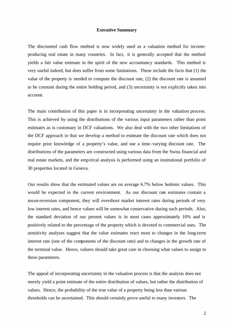
Executive Summary The discounted cash flow method is now widely used as a valuation method for income-

producing real estate in many countries. In fact, it is generally accepted that the method

yields a fair value estimate in the spirit of the new accountancy standards. This method is

very useful indeed, but does suffer from some limitations. These include the facts that (1) the

value of the property is needed to compute the discount rate, (2) the discount rate is assumed

to be constant during the entire holding period, and (3) uncertainty is not explicitly taken into

account.

The main contribution of this paper is in incorporating uncertainty in the valuation process.

This is achieved by using the distributions of the various input parameters rather than point

estimates as is customary in DCF valuations. We also deal with the two other limitations of

the DCF approach in that we develop a method to estimate the discount rate which does not

require prior knowledge of a property’s value, and use a time-varying discount rate. The

distributions of the parameters are constructed using various data from the Swiss financial and

real estate markets, and the empirical analysis is performed using an institutional portfolio of

30 properties located in Geneva.

Our results show that the estimated values are on average 6.7% below hedonic values. This

would be expected in the current environment. As our discount rate estimates contain a

mean-reversion component, they will overshoot market interest rates during periods of very

low interest rates, and hence values will be somewhat conservative during such periods. Also,

the standard deviation of our present values is in most cases approximately 10% and is

positively related to the percentage of the property which is devoted to commercial uses. The

sensitivity analyses suggest that the value estimates react most to changes in the long-term

interest rate (one of the components of the discount rate) and to changes in the growth rate of

the terminal value. Hence, valuers should take great care in choosing what values to assign to

these parameters.

The appeal of incorporating uncertainty in the valuation process is that the analysis does not

merely yield a point estimate of the entire distribution of values, but rather the distribution of

values. Hence, the probability of the true value of a property being less than various

thresholds can be ascertained. This should certainly prove useful to many investors. The

3

Royal Institution of Chartered Surveyors (RICS) in the U.K., for instance, is currently

examining how uncertainty can be used together with the value estimate, which highlights the

importance of uncertainty for the valuation profession. Also, there has been some debate in

the literature about valuation variation and the margin of error in valuing properties. The

approach which is advocated in this paper should constitute a contribution to this debate.

4

Monte Carlo Simulations for Real Estate Valuation 1. Introduction

Among the various approaches to valuing real estate, the discounted cash flow (DCF) method,

using the weighted average cost of capital (WACC) as the discount rate, is well accepted by

academics and broadly used by practitioners. The consensus derives from the model’s

advantages, in particular its economic rationality. The DCF method takes into account the

time value of money and has a unique result regardless of investors’ risk preferences (Mun,

2002). In addition, the procedure is clearly defined and can easily be used by valuers.

Although the DCF method plays a crucial role in valuation, it suffers from at least three

pitfalls. First, the traditional DCF analysis is performed under deterministic assumptions (for

a discussion, see Wofford, 1978; Mollart, 1988; French and Gabrielli, 2004). In other words,

one does not take into account uncertainty in the estimated cash flows; the entire process is

therefore devalued when forecasts do not materialise or even when inputs are slightly

manipulated (Kelliher and Mahoney, 2000; Weeks, 2003). This criticism is particularly

severe in real estate valuation since the terminal value, which is dependent on the last

forecasted free cash flow, the perpetual rate of growth and on the discount rate, is in most

cases the largest component of the present value. If such parameters are not determined very

rigorously, the estimated value of a property can be very far off its market value. When the

latter value is known, one can also say that it is easy to set parameters so as to obtain a present

value that is close to it.

Another drawback of the DCF method is that there is a circularity problem when part of the

asset is financed by debt. Indeed, the value of the asset is required to compute the WACC,

but the value of the asset is precisely what we are looking for. Finally, the discount rate is

assumed to be constant through time though research has shown that prices and returns on

financial assets are related more to changes in the required rate of return than to changes in

expected cash flows (Fama and French, 1989; Ferson and Campbell, 1991). To model the

time-varying nature of the required rate of return, Geltner and Mei (1994) and Clayton (1996)

use a vector autoregressive procedure to analyse returns on priva te real estate. The latter

5

author, for instance, finds that the risk premium on direct unsecuritised commercial real estate

varies over time and is strongly related to general economic conditions.

In this research, we use the Adjusted Present Value (APV) methodology, developed by Myers

(1974), but by adding Monte Carlo simulations. Under some assumptions, the APV method

yields the same results as the widely used DCF technique (Fernandez, 2005), but it solves the

circularity problem created by debt financ ing (Achour-Fischer, 1999). In addition, with

Monte Carlo simulations, which are based on statistical measures and probability distributions

of the variables that enter in the APV method, we address the uncertainty issue.

With the APV methodology, the discount rate represents the required rate of return for fully

equity-financed properties. Many data analyses have lead us to conclude that the Capital

Asset Pricing Model (CAPM) is in most cases not applicable to estimate this required rate of

return1. First, there are usually not sufficient historical data for direct real estate investments.

Second, an appropriate definition of the market portfolio and in particular of the relative

weight of real estate in such portfolio is difficult. Third, the returns on indirect real estate

investments may be poor proxies for direct real estate returns (Lizieri and Ward, 2000). This

problem is exacerbated when one attempts to remove the effect of leverage. Further,

historical returns may be poor proxies for expected future returns (Geltner and Miller, 2001).

Finally, as mentioned previously, most such models assume that risk is constant over time.

The contributions of the paper are as follows. First, we address formally the issue of

uncertainty in valuing real estate. This is achieved by using a Monte Carlo approach within

an APV framework. Further, our approach prevents subjective changes of the values of the

parameters used to compute the terminal value, as these are obtained by clearly defined

models or procedures. Finally, we model the discount rate by considering that it has two

components: a risk free interest rate and a risk premium. We model the interest rate by using

the Cox et al. (1985) model. Such model allows us to assume that the discount rate is not

constant through time and that it depends on the present level of interest rates and their

volatility. We suggest an innovative solution to estimate the risk premium which is assumed

to depend on a real estate market premium and on property specific attributes. The attributes

are measured by selected hedonic attributes which include the quality of location, the age and

1 A notable exception to this is Baroni et al. (2001).

6

the quality of buildings. Hence our method considers that risk is multidimensional and is not

only related to covariance with the market as posited by the CAPM. In that sense it is more

closely related to Arbitrage Pricing Theory (APT).

The Monte Carlo technique, whose name comes from the famous casino in Monaco2, was

developed by famous scientists, such as Enrico Fermi, in the 1930s when calculating the

neutron diffusion, or John von Neumann and Stanislaw Ulam who established the

mathematical basis for probability density functions (Fishman, 1999). It has been

subsequently used to solve problems related to the atomic bomb, medicine, chemistry,

astronomy or agriculture. In finance, Monte Carlo simulations have also been largely used for

many years, in particular to price derivatives, to forecast stock prices or interest rates, as well

as in capital budgeting (Dixit and Pindyck, 1994). In real estate research, authors like Pellat

(1972) and Pyhrr (1973) have used simulations – but not Monte Carlo simulations - to analyse

uncertainties related to investment forecasting. In the same vein, Mallison and French (2000)

analyse the uncertainty issues related to any valuation. The Monte Carlo simulation technique

has also been applied to forecast future cash flows in order to improve long-term decisions in

real estate (Kelliher and Mahoney, 2000; Tucker, 2001; French and Gabrielli, 2004). Our

approach differs from previous research in that we forecast a time-varying discount rate that

also includes a premium related to selected hedonic characteristics. In practice, the use of the

Monte Carlo simulation technique is quite limited, probably partly due to the mathematical

and statistical dimension of this approach3.

We apply our approach to an institutional real estate portfolio for which we have the

estimated hedonic value for each of 30 properties. This allows us to compare our simulated

values with the hedonic estimates. Overall, we find that the central values of the simulations

are quite similar (albeit lower) to the hedonic values, but the standard deviation of the present

value estimates provides for an interesting measure of risk. In addition, the sensitivity

analysis clearly shows the crucial role played by the growth rate in calculating the terminal

values, but also of long-term interest rates.

2 The mathematician Stanislaw Martin Ulam tells in an autobiography that the method was called Monte Carlo to honour his uncle who was a tenacious gambler at the Monaco casino. 3 In Switzerland, the CIFI (Centre d'Information et de Formation Immobilières) uses this approach for the valuation of real estate portfolios.

7

The remainder of the paper is organised as follows. In section 2, we briefly present the APV

methodology and highlight how it addresses some of the pitfalls of the traditional DCF

technique. Section 2 also contains a discussion of how we estimate the various components

of the APV and of the hypotheses that are made concerning the probability distributions of

variables. The data and some descriptive statistics are presented in section 3, while section 4

contains the results of Monte Carlo simulations and of their sensitivity. Section 5 concludes.

2. Method

The APV methodology postulates that an asset has a value under perfect market conditions

plus, possibly, an additional value resulting from market imperfections. Considering among

market imperfections only the debt financing and using forecasted cash flows for a finite time

horizon, the value of a property can be written as follows:

( ) ( ) ( )Tu

TT

tt

i

T

tt

u

t

kTV

ktDik

kFCF

PV+

++

−∗∗+

+= ∑∑

== 111

1 110

τ (1)

where

PV0 = value of the property at time t=0

FCFt = free cash-to-property at time t (t = 1 to T)

Dt = value of debt at time t

TVT = terminal value at time T

ku = cost of capital for a fully equity-financed property

ki = pre-tax cost of debt

τ = tax rate

The advantage of equation (1) above the standard DCF formula with the average cost of

capital as the discount rate is that it considers the debt financing effects separately and

consequently resolves the circularity problem. Moreover, the free cash flows are discounted

at a rate that can be obtained from pension funds, as such investors in many countries

(including Switzerland) buy properties without any leverage. When institutional investors are

tax-exempt, which is the case in Switzerland but in many other countries as well, the present

value of the tax shield is zero and equation (1) reduces to:

( ) ( )T

u

TT

tt

u

t

kTV

kFCF

PV+

++

= ∑= 111

0 (2)

8

As the focus of this paper is the valuation of an institutional portfolio, we use equation (2) to

compute the present value of a property. This requires that the behaviour of the parameters

that enter into the formula be modelled: (1) the annual free cash flows during the forecasting

period, (2) the terminal value at the end of the forecasting period and (3) the discount rate.

For the sake of simplicity we will use the same model regardless of whether the properties are

entirely residential or whether some fraction of the property is devoted to other uses. Swiss

institutional investors predominantly purchase residential properties, with such use accounting

for approximately 85% of their real estate holdings.

2.1 Free cash flows (FCF)

For tax-exempt investors, the free cash flow to property for year t can by written as:

ttttt CAPEXC)PGI?FCF −−−= 1( (3)

where

νt = vacancy rate in year t

PGIt = potential gross income in year t

Ct = operating cash expenses in year t

CAPEXt = additional investment (ie capital expenses) in year t

Rents are the major source of cash inflows and they depend on future market conditions, the

characteristics of the properties, but also on various legal constraints. The potential gross

income (PGI) for the first year (Year 1) is assumed to be known for the various components

of the property (apartments, underground garages, shops, etc.). We then assume that the

growth of the PGI over time is normally distributed. The choice of the mean and the standard

deviation of the growth rate is crucial. Growth will depend not only on macroeconomic

factors such as expected GDP growth, expected inflation or demographic phenomena, but also

on property-specific characteristics such as the quality or the age of building, but also the

quality of location. The actual level of rents partly captures theses variables, but we have to

recognise that the appropriate future growth rate for a well located and well constructed new

building might be quite different from the rate applicable to a low quality and poorly located

old building. From a theoretical point of view, it would be better if various growth rates could

be considered, but in practice these are very difficult to estimate. The growth rate of rents is

one of the key drivers of property values and therefore its estimation should rely on a

9

procedure that is as objective as possible. In this paper, we use historical data to proxy for

future growth rates.

The level of the cash inflow is also a function of a specific type of risk related to real estate

investment, ie the vacancy rate (υ). We will assume that the latter is uniformly distributed

between the historical minimum and maximum vacancy rates for similar properties. By

multiplying the PGI by (1-?), we obtain the rent or total rent, ie the amount of cash inflow that

is expected from renting out the property. For the sake of simplicity, we omit to explicitly

consider the rate of unpaid rent (ie tenants who do not pay their rent), which implies that the

PGI is net of unpaid rent.

Cash outflows include operating expenses, property taxes, insurance, and utilities. These are

largely fixed, ie they will occur whether the property is or is not fully occupied. The variable

component of these expenses is largely dependent on the age of the building, such that we will

model the uncertain part of these expenses as a function of both age and rent. Historical data

and professional expertise can help determine the level of annual fixed expenses as a

percentage of rents and be useful in creating a model to estimate variable expenses. If

sufficient data were available, one could also model the level of operating expenses by

including other independent variables, such as the building quality or the quality of recent

improvements.

Additional investments have to be forecasted to maintain or to improve the quality of the

properties, or in some cases to increase their size. The amounts taken into consideration

should be those that are forecasted by the owner, preferably with the help of an architect who

has received a clear mandate to estimate the future investments required to reach the goals set

above. In some countries or cities, due to legal restrictions to rent increases, one difficulty

will then be to model future cash flows which depend on such additional investments.

2.2 Terminal value

The terminal value should be a proxy for the market value of the property at the end of the

forecasting period under normal market conditions. We use Gordon’s growth model which is

often used both by academics (Damodaran, 2003; Geltner and Miller, 2001) and

professionals. To avoid obtaining aberrant terminal value estimates, it is important to first

“normalize” the free cash flow of the last year of the horizon period. As we rely on a model

10

to forecast future cash flows, we will use the arithmetic mean of the free cash flows of the last

three years to proxy for the normalized free cash to property of the last year. As is the case

for the cost of capital, the perpetual rate of growth is highly related to the inflation rate. The

residual life of a building is limited, however, such that the rate of growth will sooner or later

become negative. Consequently, in countries where inflation is low, the rate of growth is low

or even set equal to zero. If not, the resulting estimated terminal value is too high,

considering the level of PGI at the end of the forecasted period. In other words, we argue that

it is possible, and in some cases preferable, to estimate the terminal value by using the gross

income multiplier that prevails under normal market conditions.

We calculate the terminal value as4:

gk

gFCFFCFFCF

gkFCF

TVu

TTT

u

TT −

+++

=−

=

−−

+)1(

3)( 21

1 (4)

where

FCFT+1 = free cash flow of period T+1

ku = discount rate

g = perpetual growth rate of the free cash flows

2.3 Discount rate

To forecast the expected return on real estate, we assume that the discount rate is time-varying

and dependent on market interest rates. We first assume that the discount rate for a fully

equity-financed property is higher than the risk free interest rate (thereafter interest rate)

observed on the market, but lower than the historical return of stocks. Thus, the following

inequality is assumed to hold:

ir < ku < k s (5)

where

ir = interest rate observed on the market

ku = required rate of return for a fully equity-financed property

ks = historical rate of return of the stock market

4 Baroni et al. (2001) simulate the paths of the terminal value using a geometric Brownian motion. This method, however, requires that the initial value be known. We cannot use this method as the initial value (ie the estimated value) is precisely what we are looking for.

11

We then compute the discount rate, ku, as the sum of the interest rate plus a risk premium that

is required by investors. Thus:

ir <( ku = ir + P) < k s (6)

where P is the risk premium. The procedure used to set the interest rate and the risk premium

is discussed next.

2.3.1 Interest rate model

The interest rate used should be highly correlated to the mortgage interest rate. In

Switzerland, until the 1990s, the reference for mortgage rates was the savings deposit rate

paid to customers plus a margin (Bruand, 1998)5. During the 1990s, some banks, in particular

large banks, shifted toward another strategy, using the money market rates, such as the 3- or

6-month Libor, as the reference for the mortgage rate.

There exist various models to forecast interest rates and, in general, these have two

components: the drift and the volatility. One of the most widely used model is that of Cox et

al. (1985), thereafter CIR:

drt = a(b – rt)dt + tr s dWt (7)

where

drt = increment in the interest rate at time t

a = a non-negative constant (the mean-reversion speed)

b = a constant (the long-term equilibrium interest rate)

σ = the volatility of the interest rate

dWt = the Wiener increment, tdttt WWdW −= +

The drift term implies that the interest rate normally will rise when it is below the long-term

mean, and that it will normally fall when it is above the mean. The discrete approximation of

the CIR model is as follows:

( ) trtrbr ∆+∆−=∆ εσα (8)

where ε à N(0,1).

5 Bruand (1998) created a model to determine the mortgage rate for Switzerland using 6-month Eurofranc money market rates. The adjustment process, which is undertaken at most twice yearly, occurs when the trend in the movement of the interest rate is confirmed. By adopting a filter to 6-month Eurofranc rates, Bruand obtains the series of mortgage rate changes. Our objective being to forecast the interest rate levels, we will not use any filter.

12

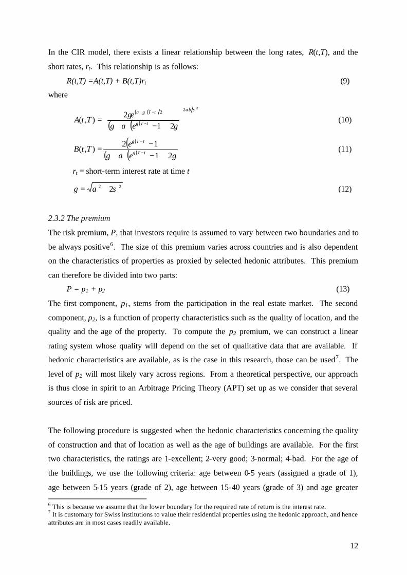
In the CIR model, there exists a linear relationship between the long rates, R(t,T), and the

short rates, rt. This relationship is as follows:

R(t,T) =A(t,T) + B(t,T)rt (9)

where

( )( )

( ) ( )( )222

212

),(σα

γ

γα

γαγγ

b

tT

tT

ee

TtA

+−+

= −

−+

(10)

( )( )( ) ( )( ) γαγ γ

γ

2112

),(+−+

−= −

−

tT

tT

ee

TtB (11)

rt = short-term interest rate at time t

22 2σαγ += (12)

2.3.2 The premium

The risk premium, P, that investors require is assumed to vary between two boundaries and to

be always positive6. The size of this premium varies across countries and is also dependent

on the characteristics of properties as proxied by selected hedonic attributes. This premium

can therefore be divided into two parts:

P = p1 + p2 (13)

The first component, p1, stems from the participation in the real estate market. The second

component, p2, is a function of property characteristics such as the quality of location, and the

quality and the age of the property. To compute the p2 premium, we can construct a linear

rating system whose quality will depend on the set of qualitative data that are available. If

hedonic characteristics are available, as is the case in this research, those can be used7. The

level of p2 will most likely vary across regions. From a theoretical perspective, our approach

is thus close in spirit to an Arbitrage Pricing Theory (APT) set up as we consider that several

sources of risk are priced.

The following procedure is suggested when the hedonic characteristics concerning the quality

of construction and that of location as well as the age of buildings are available. For the first

two characteristics, the ratings are 1-excellent; 2-very good; 3-normal; 4-bad. For the age of

the buildings, we use the following criteria: age between 0-5 years (assigned a grade of 1),

age between 5-15 years (grade of 2), age between 15-40 years (grade of 3) and age greater 6 This is because we assume that the lower boundary for the required rate of return is the interest rate. 7 It is customary for Swiss institutions to value their residential properties using the hedonic approach, and hence attributes are in most cases readily available.

13

than 40 years (grade of 4). We then assume that the quality of the building and that of

location are more valuable features for an investor than the age of the building, so that we

assign a 40% weight to each of the first two characteristics and a weight of 20% to age. We

assign 100 points for a grade of 1; 75 points for a grade of 2; 50 points for a grade of 3 and 25

points for a grade of 4. The total number of points (TP) is given by:

TP = w(building quality)*P(building quality) + w(location)*P(location) +

w(age)*P(age) (14)

where w is the weight and P the number of points.

The value of p2 is then calculated as:

p2 = (100 - TP) / 100 (15)

To illustrate, consider a building of high quality (grade of 1), with an average quality location

(grade of 3) and constructed 18 years ago (grade of 3). Therefore, TP = 40%*100 + 40%*50

+ 20%*25 = 65 points. Then, the premium p2 would be equal to (100-65)/100 = 0.45%. In

contrast, the p2 premium for a luxurious new building with an excellent location will be zero.

Although this system is somewhat arbitrary, it makes sense and is consistent with the hedonic

approach. As a general rule, high quality properties are likely to be occupied by more secure

tenants and are viewed as less risky by investors (Gunnelin et al., 2004).

2.4 Correlations and other considerations

In addition to being uncertain, the variables used in the valuation process are not completely

independent from each other. For example, rents and property prices may be correlated such

that we should take into consideration their co-movements when performing our simulations.

Historical data on the evolution of property prices and rents should constitute a good indicator

for future correlations. What about the correlations between interest rates and property prices

or between interest rates and rents? From a theoretical point of view, an interest rate increase

should induce a decrease in property prices, and vice versa. However, an interest rate

increase not only induces a rise of interest expenses, but also of the cost of equity, and

therefore there will be a pressure to increase rents. We hypothesise a positive correlation

between mortgage rates and rents, and a negative correlation between vacancy rates and rents.

Further, it seems reasonable to assume that p1 is higher when interest rates are low and vice

versa, which means that there is a negative correlation between the two series.

14

In many countries, rent adjustments are possible to compensate for changes in interest rates,

though we observe that the adjustments for interest increases are in most cases more

systematic than adjustments for interest decreases. However, as many laws do not allow

adjustment beyond certain limits, rent adjustments are constrained (for Geneva, see Aziz et

al., 2005). The same is often true when major capital expenditures are undertaken, ie rents

cannot be increased for the return on the invested capital to remain constant.

In summary, we perform the following steps to run the Monte Carlo simulations: (1) we

estimate the free cash flows by means of equation (3) and calculate single point estimates of

future free cash flows using a probability density function for each of the components of the

free cash flow; (2) we calculate a term structure of interest rates using equations (9), (10), (11)

and (12); (3) we compute the premium P = p1+ p2 and add it to the rate calculated in step (2);

and (4) we estimate the terminal value using equation (4). This procedure yields a single

point estimated value. The procedure is then repeated 50,000 times to yield a distribution of

possible property values.

3. Data

We apply our valuation methodology to the real estate portfolio of a tax-exempt Swiss

institutional investor. The portfolio contains 30 properties with an estimated market value in

excess of CHF 237 million (Euros 160 million) as of the end of 2004. Most of the properties

are residential buildings, but some also contain office or retail uses. The time horizon for the

forecasting period is set at ten years. We provide the detailed computations for a 50-year old

and well constructed building which has a good location (Building “Edelweiss”). A capital

expenditure of CHF 150,000 is forecasted in year 3. From the first year pro formas, it appears

that the annual rent for residential use is CHF 4,500 per room8. In addition, the building

contains retail premises yielding a first-year rent of CHF 150,000. Table I reports selected

building and financial characteristics.

8 It would be better to use the rent per square meter criterion, but in Geneva the rent per room criterion is commonly used even in laws and in administrative documents (note that a kitchen is considered as being a room).

15

Statistical data available in Switzerland concerning rent levels and changes are unfortunately

not very useful for our study, as there is only one global index for the whole country. Instead,

we rely on real estate price indices, which are calculated for various regions of the country, to

proxy for the mean and standard deviation of rental growth. By doing so, we have estimates

concerning the Geneva area for the period 1971-2004, for both old and new buildings and for

several property uses. Table II contains summary statistics for real estate capital returns in

Geneva. All data, computed by Wuest & Partners, are obtained from the Swiss Federal Office

of Statistics. New residential buildings exhibit higher return and risk characteristics than old

buildings, and commercial properties appear to command lower capital returns but higher risk

than residential properties. The volatility of workshop returns is particularly high.

Vacancy rates (Table III), calculated by the Swiss National Bank, are available for 1975-2004

but unfortunately only at the national level. They were low during the whole period, which is

typical of the Swiss residential real estate market. More refined statistics would probably

highlight differences between rural areas and urban agglomerations such as Zurich, Geneva or

Basel.

Cash operating expenses are set as a percentage of gross potential income, based on historical

data taken from the real estate portfolio which is used for the empirical investigation in this

paper, as well as on estimates that were provided by professionals for residential buildings in

the Geneva area. The fixed component is set at 10% of rents. The variable component, which

is between 5-20% of rents, is related to age in the following manner: 15-20% for buildings

older than 40 years, 10-15% for buildings between 10 and 40 years old and 5-10% for

buildings less than 10 years old. These cut-offs are obviously somewhat arbitrary, but at least

they show that operating expenses and therefore operating cash flows are a function of the age

of the buildings. Operating expenses are assumed to follow a triangular distribution, with a

most likely value of 22.5%. As far as capital expenditures are considered, we obtained

detailed information about their date of occurrence in the future and their forecasted amounts.

The modelling of such behaviour is beyond the scope of this paper however. Rent rises

subsequent to capital expenses are also assumed to follow triangular distributions. Note that

we distinguish between two types of capital expenditures (ie minor and major expenditures).

An expense is defined as major when it exceeds the annual rental income in a given year.

Distributional assumptions appear in Table I.

16

We use 6-month Eurofranc rates for the 1974-2004 period to apply the CIR model and the

Swiss Market Equity Index at the end of each quarter to determine the maximum level of the

risk premium (P). Both sets of data are taken from Datastream (see Table III). The

Datastream Market Index, which is a capital weighted index which includes all firms traded

on the Swiss exchange (SWX), exhibited strong returns during the period with a mean annual

return of approximately 10%. The average interest rate was 3.1% during the 1974-2004

period (the rate in table III is an annualised rate).

The premium P is assumed to vary between 0 and 2.5%. The first component (p1) is assumed

to vary between 0 and 1.5%. We opt for a truncated normal distribution with a mean of

0.075%, a standard deviation of 1%, a minimum of 0% and a maximum of 1.5%. The second

component (p2), which is a function of the hedonic characteristics of properties, varies

between 0-1%. For each property, we compute p2 according to the procedure described in

section 2.

The central value of the 0-2.5% range is consistent with the premium required for real estate

investments by pension funds in Geneva. It is worthwhile to dig deeper into the required risk

premium to examine its relation with historical risk premia in Switzerland. At the portfolio

level (and a fortiori at the market level), the premium P will be comprised of p1 and a level of

p2 in line with the portfolio attributes. As buildings in a portfolio cannot all be new, of

excellent quality and located in excellent areas, the average value of p2 will be in the 0.5-

0.75% range. If we consider the average of the 0-1.5% range for p1 (ie 0.75%), the average

risk premium is approximately 1.25-1.5%. A comparison of that figure with the historical

return on real estate at the national level net of the interest rate level provides for a useful

check of our assumptions. Hoesli and Hamelink (2004) find that real estate in Switzerland

yielded an average return of 5.3% for the period 1979-2002. Considering that 6-month

Eurofranc rates have exhibited an average of 3.1% over the last 30 years, our assumptions

seem plausible.

The correlations between variables are impossible to obtain due to lack of data. Based on

good judgement, we consider a negative correlation of –0.5 between the premium p1 and the

interest rates and a negative correlation of –0.75 between the rental growth rate and the

vacancy rate. In addition, we consider a positive correlation of 0.5 between rents and

operating expenses.

17

4. Results In this section, we present our results both for the portfolio of 30 properties and for building

“Edelweiss”. The starting point for any valuation using our method is to estimate the term

structure of interest rates. Using conditional maximum likelihood estimation on historical 6-

month Eurofranc interest rates to compute the various parameters of equation (9), we obtain

the results that appear in Table IV. These parameters (pullback, long-term equilibrium and

instantaneous standard deviation) are significantly different from zero and are close to those

obtained by Bruand (1998) for the period 1975-1995. We do not check for the stability of

these parameters for sub-periods as this would be beyond the objective of this paper. We then

calculate the term structure of interest rates with the help of equations (9), (10), (11) and (12)

(see Figure I). As the initial interest rate is very low (less than 1%) and the equilibrium long-

term rate is 4% (b parameter in Table IV), the term structure is upward slopping.

To each estimated interest rate we add the risk premium, P= p1+ p2. As already mentioned, p1

is assumed to follow a truncated normal distribution with a mean of 0.05%, a standard

deviation of 1%, a minimum of 0 and a maximum of 1.5%. The property-specific premium p2

for building “Edelweiss” is obtained as follows: as the building has a very good location

(grade of 2), is of excellent quality (grade of 1) and is older than 40 years (grade of 4), we

assign 40%*100 + 40%*75 + 20%*25 = 75 points to the building. The p2 premium is thus

equal to (100-75)/100 = 0.25%.

Knowing the discount rates and all components of the free cash flows, we run the simulations

(50,000 iterations) and obtain for each building the distribution of present values. The

interpretation of the distribution of present values is straightforward. The range of possible

present values and the shape of the distribution reflect the uncertainty issues related to the

valuation of each property. For building “Edelweiss”, the distribution and the statistics of that

distribution are given in Figure II. We observe that the mean present value for the building is

CHF 5.67 million and the standard deviation CHF 0.6 million. The results span from a low of

CHF 3.3 million to a high of CHF 7.9 million, which represents a range of more than CHF 4.5

million. However, 90% of the present values are between CHF 4.58-6.75 million, which is a

much tighter range, ie about half the range of all possible outcomes.

18

The importance of the shape and of the range of possible outcomes varies according to the

objectives of the persons using the real estate valuations. Banks granting mortgage loans may

be more interested by the whole range of present values on the le ft hand side of the

distribution to analyse the likelihood that the value of the building would fall below some

threshold. Knowing this likelihood should help them set the interest rate that they will charge.

In contrast, the borrower may be more inclined not to argue with the banker on the basis of

the whole range of values to the left of the mean value, but rather to advocate using only part

of the range of values as it is unlikely that the market value of the property will decline

drastically over some given time horizon. The same behaviour may be observed for the seller

of a property or a real estate portfolio manager. In this respect, the concept of Value-at-Risk

(VaR) would be useful as it would provide an estimate of the maximum loss for various time

horizons (see Baroni et al., 2001).

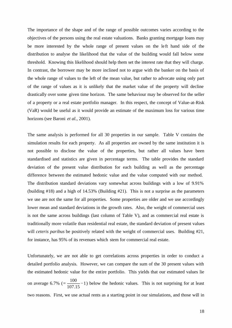
The same analysis is performed for all 30 properties in our sample. Table V contains the

simulation results for each property. As all properties are owned by the same institution it is

not possible to disclose the value of the properties, but rather all values have been

standardised and statistics are given in percentage terms. The table provides the standard

deviation of the present value distribution for each building as well as the percentage

difference between the estimated hedonic value and the value computed with our method.

The distribution standard deviations vary somewhat across buildings with a low of 9.91%

(building #18) and a high of 14.53% (Building #21). This is not a surprise as the parameters

we use are not the same for all properties. Some properties are older and we use accordingly

lower mean and standard deviations in the growth rates. Also, the weight of commercial uses

is not the same across buildings (last column of Table V), and as commercial real estate is

traditionally more volatile than residential real estate, the standard deviation of present values

will ceteris paribus be positively related with the weight of commercial uses. Building #21,

for instance, has 95% of its revenues which stem for commercial real estate.

Unfortunately, we are not able to get correlations across properties in order to conduct a

detailed portfolio analysis. However, we can compare the sum of the 30 present values with

the estimated hedonic value for the entire portfolio. This yields that our estimated values lie

on average 6.7% ( 115.107

100−= ) below the hedonic values. This is not surprising for at least

two reasons. First, we use actual rents as a starting point in our simulations, and those will in

19

many cases be less than market rents as rents charged to current tenants only adjust

imperfectly to market rents. Second, our estimated discount rates constitute long-term

trending rates and as such should yield more conservative value estimates than if current

(historically very low) rates were to be used.

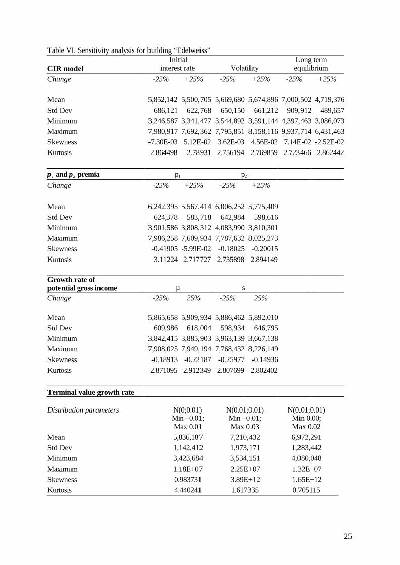
In a next step, we perform a sensitivity analysis to gauge the impact on the present value of

changes in input parameters for building “Edelweiss” (Table VI). For all uncertain

parameters, we examine the impact of a 25% decrease and 25% increase, respectively, in the

initial values. These include the initial interest rate, the volatility and the long term

equilibrium in the CIR model, both components of the risk premium (ie p1 and p2), the mean

and standard deviation of the potential gross income and the terminal value growth rate. For

instance, if the initial interest rate in the CIR model is 0.8%, then we perform our sensitivity

analysis using values of 0.8%*1.25 = 1% and 0.8%*0.75= 0.6%, respectively.

The sensitivity analysis results show that a change in the long-term equilibrium rate has a

strong impact on the estimated value due to the impact on the discount rate. For example, if

the long-term rate in the CIR model decreases to 3% (a decrease of 25% from the initial value

of 4%), this translates into an increase to CHF 7 million of the mean present value of the

building (CHF 5.7 million in the original simulation). The components of the premium above

interest rates also have an important impact on the present value, albeit less important than the

long-term equilibrium rate.

The estimated growth rate of the terminal value also has a substantial impact on the estimated

values. Recall that in our base scenario we adopted a zero growth model after the 10th year of

the horizon period. When we drop this hypothesis, and consider truncated normal

distributions for the growth rate, we obtain insightful results. Three hypotheses are

considered and the impact of these is reported in the bottom part of Table VI. As the mean of

the growth rate increases, so does the mean of the present value. Not surprisingly, we observe

higher maximum present values (CHF 13 million) when the growth rate of the cash flows

beyond period t = 10, is assumed to have a mean of 1% per year and the rate is truncated

between 0 and 2%. If the upper limit for the growth rate is set at 3%, then the maximum

present value exceeds CHF 22 million. Valuers would be very hard pressed however using

such a growth rate in Switzerland given the structure and constraints of the residential market.

20

Interestingly, our present values appear to be less sensitive to changes in the risk premia and

even less so to changes in the potential gross income rate of growth.

5. Conclusions

The discounted cash flow method is now widely used as a valuation method for income-

producing real estate in many countries. In fact, it is generally accepted that the method

yields a fair value estimate in the spirit of the new accountancy standards. This method is

very useful indeed, but does suffer from some limitations. These include the facts that (1) the

value of the property is needed to compute the discount rate, (2) the discount rate is assumed

to be constant during the entire holding period, and (3) uncertainty is not explicitly taken into

account.

The main contribution of this paper is in incorporating uncertainty in the valuation process.

This is achieved by using the distributions of the various input parameters rather than point

estimates as is customary in DCF valuations. We also deal with the two other limitations of

the DCF approach in that we develop a method to estimate the discount rate which does not

require prior knowledge of a property’s value, and use a time-varying discount rate. The

distributions of the parameters are constructed using various data from the Swiss financial and

real estate markets, and the empirical analysis is performed using an institutional portfolio of

30 properties located in Geneva.

Our results show that the estimated values are on average 6.7% below hedonic values. This

would be expected in the current environment. As our discount rate estimates contain a

mean-reversion component, they will overshoot market interest rates during periods of very

low interest rates, and hence values will be somewhat conservative during such periods. Also,

the standard deviation of our present values is in most cases approximately 10% and is

positively related to the percentage of the property which is devoted to commercial uses. The

sensitivity analyses suggest that the value estimates react most to changes in the long-term

interest rate (one of the components of the discount rate) and to changes in the growth rate of

the terminal value. Hence, valuers should take great care in choosing what values to assign to

these parameters.

21

The appeal of incorporating uncertainty in the valuation process is that the analysis does not

merely yield a point estimate of the entire distribution of values, but rather the distribution of

values. Hence, the probability of the true value of a property being less than various

thresholds can be ascertained. This should certainly prove useful to many investors. The

Royal Institution of Chartered Surveyors (RICS), for instance, is currently examining how

uncertainty can be used together with the value estimate, which highlights the importance of

uncertainty for the valuation profession. Also, there has been some debate in the literature

about valuation variation and the margin of error in valuing properties (Adair et al., 1996;

Crosby et al., 1998). The approach which is advocated in this paper should constitute a

contribution to this debate.

As is the case of all techniques, the quality of the outputs from a Monte Carlo simulation

largely depends on the quality of the inputs (Li, 2000). With this in mind, further research

should focus on the stability of the model that we use when other portfolios are used and for

different periods of the real estate cycle. In particular, when the real estate market will be

bearish again, it will be of interest to compare estimated values to hedonic values or to

estimates generated using other valuation methods. Also, further investigation of which

property attributes should be considered when constructing the property-specific risk

premium and of how these mostly qualitative attributes should be weighted is warranted.

Finally, it would seem fruitful to dig deeper in the relation between capital expenses and

property values. This could suggest optimal time windows for undertaking such expenses

during the life cycle of buildings. In doing so, a better understanding of the linkages between

capital expenses and various other variables should emerge.

22

Table I. Building and financial characteristics and parameter probability distributions for building “Edelweiss”

2 rooms 3 rooms 3.5 rooms 5.5 rooms Number of flats 6 2 4 6 Total number of rooms 12 6 14 33 Price per room CHF 4,500 City Geneva Age >50 years Quality of location Good Building quality Excellent

Residential Use Distribution Parameters Rental growth rate

Normal

Historical mean and volatility for real estate capital returns on residential buildings in the Geneva area

Vacancy rate

Uniform

Historical minimum and maximum for vacancy rates in Switzerland

Operating expenses

Triangular

Minimum 15% of rents, maximum 30%, most likely value 23%

Rent rise when major CAPEX Triangular Minimum 0, maximum 10%, most likely value 7.5% Rent rise when minor CAPEX Triangular Minimum 0, maximum 5%, most likely value 3.5%

Commercial Use Potential Gross Income (annual)

CHF 150,000

Distribution Parameters Commercial rental growth rate

Normal

Historical mean and volatility for real estate capital returns on commercial buildings in Switzerland

Vacancy rate Uniform Minimum of 4% and maximum of 8% Operating expenses

Triangular

Minimum 15% of rents, maximum 30%, most likely value 23%

Rent rise when major CAPEX Triangular Minimum 0, maximum 15%, most likely value 10% Rent rise when minor CAPEX Triangular Minimum 0, maximum 10%, most likely value 7.5%

23

Table II. Descriptive data for real estate capital returns in Geneva, 1971-2004

Mean Std Min Max N

Panel A. Residential Old buildings 0.032 0.086 -0.115 0.22 34 New buildings 0.048 0.094 -0.086 0.272 34

Panel B. Commercial Offices 0.023 0.096 -0.193 0.352 34

Workshops 0.028 0.209 -0.718 0.534 34 Retail 0.016 0.096 -0.147 0.293 34

Table III. Descriptive statistics for the vacancy rate, 6-month Eurofranc rate and Datastream Stock Market Index for Switzerland, for the period 1974-2004 (1975-2004 for vacancy rates), various frequencies

Data type Frequency Mean Std Min Max N

Vacancy rate Yearly 0.010 0.005 0.004 0.018 30 6-month Eurofranc rate Monthly 0.031 0.006 0.013 0.043 372

DS stock returns Quarterly 0.025 0.112 -0.420 0.208 124

Table IV. Conditional maximum likelihood estimation for interest rates (CIR model) Frequency Log L a b s N

Monthly 841 0.480 0.040 0.021 372

(2.89) (4.18) (9.51)

Note: a is the pullback, b is the long term equilibrium and s the instantaneous standard deviation, t-stats in parentheses

24

Table V. Standard deviation of present values, percentage difference with hedonic values and property uses (portfolio of 30 properties)

Building # Std deviation of

PV (%) Hedonic/Mean of Present Value (%)

Residential (%) Commercial (%)

1 11.36 4.37 62 38 2 11.12 11.23 76 24 3 9.94 17.12 100 0 4 10.51 2.06 94 6 5 10.15 7.94 99 1 6 10.33 -5.81 98 2 7 11.18 -3.44 76 24 8 10.88 15.33 86 14 9 9.94 -7.15 100 0

10 11.00 6.15 85 15 11 9.94 -18.08 100 0 12 10.57 11.22 92 8 13 11.06 22.41 78 22 14 10.45 -6.75 95 5 15 11.53 9.26 61 39 16 11.30 3.34 67 33 17 11.24 10.67 73 27 18 9.91 7.54 100 0 19 10.27 6.70 98 2 20 10.70 6.57 87 13 21 14.53 20.29 5 95 22 10.39 7.14 97 3 23 10.94 4.70 85 15 24 11.66 11.04 61 39 25 10.63 12.71 87 13 26 13.37 -5.49 41 59 27 10.21 0.77 99 1 28 10.76 5.18 86 14 29 10.09 13.81 99 1 30 10.82 13.01 86 14

All properties 7.15

25

Table VI. Sensitivity analysis for building “Edelweiss”

CIR model Initial

interest rate Volatility Long term equilibrium

Change -25% +25% -25% +25% -25% +25% Mean 5,852,142 5,500,705 5,669,680 5,674,896 7,000,502 4,719,376Std Dev 686,121 622,768 650,150 661,212 909,912 489,657Minimum 3,246,587 3,341,477 3,544,892 3,591,144 4,397,463 3,086,073Maximum 7,980,917 7,692,362 7,795,851 8,158,116 9,937,714 6,431,463Skewness -7.30E-03 5.12E-02 3.62E-03 4.56E-02 7.14E-02 -2.52E-02Kurtosis 2.864498 2.78931 2.756194 2.769859 2.723466 2.862442 p1 and p2 premia p1 p2 Change -25% +25% -25% +25% Mean 6,242,395 5,567,414 6,006,252 5,775,409 Std Dev 624,378 583,718 642,984 598,616 Minimum 3,901,586 3,808,312 4,083,990 3,810,301 Maximum 7,986,258 7,609,934 7,787,632 8,025,273 Skewness -0.41905 -5.99E-02 -0.18025 -0.20015 Kurtosis 3.11224 2.717727 2.735898 2.894149 Growth rate of potential gross income µ s Change -25% 25% -25% 25% Mean 5,865,658 5,909,934 5,886,462 5,892,010 Std Dev 609,986 618,004 598,934 646,795 Minimum 3,842,415 3,885,903 3,963,139 3,667,138 Maximum 7,908,025 7,949,194 7,768,432 8,226,149 Skewness -0.18913 -0.22187 -0.25977 -0.14936 Kurtosis 2.871095 2.912349 2.807699 2.802402

Terminal value growth rate Distribution parameters

N(0;0.01) Min –0.01; Max 0.01

N(0.01;0.01) Min –0.01; Max 0.03

N(0.01;0.01) Min 0.00; Max 0.02

Mean 5,836,187 7,210,432 6,972,291 Std Dev 1,142,412 1,973,171 1,283,442 Minimum 3,423,684 3,534,151 4,080,048 Maximum 1.18E+07 2.25E+07 1.32E+07 Skewness 0.983731 3.89E+12 1.65E+12 Kurtosis 4.440241 1.617335 0.705115

26

Figure I. Term structure of interest rates

Term structure

0

0.005

0.01

0.015

0.02

0.025

0.03

0.035

0.04

0.045

1 2 3 4 5 6 7 8 9 10 11 12 13 14 15 16

Time

Inte

rest

rat

e

Interest rate

Long term equilibrium

Figure II. Distribution of the present value for building “Edelweiss”

Minimum 3335127 Mean 5672066 Maximum 7786397 Std Dev 644320 Skewness -0.00715 Kurtosis 2.823

Mean = 5672066

X <=45773865%

X <=675061195%

0

1

2

3

4

5

6

7

3 4.25 5.5 6.75 8

Values in Millions

27

References Achour-Fischer, D. (1999), “Is there a Myers way to value income flows?”, Working paper,

Curtin Business School, Perth. Adair, A., Hutchison, N., MacGregor, B., McGreal, S. and Nanthakumaran, N. (1996), “An

analysis of valuation variation in the UK commercial property market: Hager and Lord revisited”, Journal of Property Valuation and Investment, Vol. 14 No. 5, pp. 34-47.

Aziz, N., Bender, A. and Hoesli, M. (2005), “Evaluation immobilière par les DCF”, L’Expert-comptable suisse, Vol. 79 No. 5, pp. 345-355.

Baroni, M., Barthélémy, F. and Mokrane, M. (2001), “Volatility, Monte-Carlo simulations and the use of option pricing models in real estate”, Working paper, ESSEC, Paris.

Bruand, M. (1998), “Pricing and hedging caps on the Swiss Index of mortgage rates”, The Journal of Fixed Income, Vol. 7 No. 4, pp. 94-111.

Clayton, J. (1996), “Market fundamentals, risk and the Canadian property cycle: Implications for property valuation and investment decisions”, The Journal of Real Estate Research, Vol. 12 No. 3, pp. 347-367.

Cox, C.J., Ingersoll, J.E. and Ross, S.A. (1985), “A theory of the term structure of interest rates”, Econometrica, Vol. 53 No. 2, pp. 385-407.

Crosby, N., Lavers, A. and Murdoch, J. (1998), “Property valuation variation and the ‘margin of error’ in the UK”, Journal of Property Research, Vol. 15 No. 4, pp. 305-330.

Damodaran, A. (2002), Investment Valuation: Tools and Techniques for Determining the Value of Any Asset, Wiley, New York.

Dixit, A. and Pindyck, R. (1994), Investment Under Uncertainty. Princeton University Press, Princeton, NJ.

Fama, E. and French, K. (1989), “Business conditions and expected returns on stocks and bonds”, Journal of Financial Economics, Vol. 25 No. 1, pp. 23-49.

Fernandez, P. (forthcoming 2005), “Equivalence of ten different methods for valuing companies by cash flow discounting”, International Journal of Financial Education.

Ferson, W. and Campbell, R.H. (1991), “The variation of economic risk premiums”, Journal of Political Economy, Vol. 99 No. 2, pp. 385-415.

Fishman, G.S. (1999), Monte Carlo: Concepts, Algorithms, and Applications, Springer series in operations research, Springer-Verlag, New York.

French, N. and Gabrielli, L. (2004), “The uncertainty of valuation” Journal of Property Investment & Finance, Vol. 22 No. 6, pp. 484-500.

Geltner, D. and Mei, J. (1994), “The present value model with time varying discount rates: Implications for commercial property valuation and investment decisions”, RERI. Available http://www.ncreif.com/committees/pdf/The_Present_Value_Model_with_Time_Varying_Discount_Rates_Imp.pdf

Geltner, D. and Miller, N.G. (2001), Commercial Real Estate Analysis and Investments, Prentice-Hall, New Jersey.

Gunnelin, Å., Hendershott, P.H., Hoesli, M. and Söderberg, B. (2004), “Determinants of cross-sectional variation in discount rates, growth rates and exit cap rates”, Real Estate Economics, Vol. 32 No. 2, pp. 217-237.

Hoesli, M. and Hamelink, F. (2004), “Portefeuilles institutionnels suisses et immobilier européen”, L’Expert-comptable suisse, Vol. 78 No. 8, pp. 637-643.

28

Kelliher, C.F. and Mahoney, L.S. (2000), “Using Monte Carlo simulation to improve long-term investment decisions”, The Appraisal Journal, Vol. 68 No. 1, pp. 44-56.

Li, H.L. (2000), “Simple computer applications improve the versatility of discounted cash flow analysis”, The Appraisal Journal, Vol. 68 No. 1, pp. 86-92.

Lizieri, C. and Ward, C. (2000), “The distribution of real estate returns” in Knight, J, and Satchell, S. (Eds.), Return Distributions in Finance, Butterworth Heinemann, Oxford, pp. 47-74.

Mallison, M. and French, N. (2000), “Uncertainty in property valuation”, Journal of Property Investment & Finance, Vol. 18 No. 1, pp. 13-32.

Mollart, R.G. (1988), “Monte Carlo simulation using LOTUS 123”, Journal of Property Valuation, Vol. 6 No. 4, pp. 419-433.

Mun, J. (2002), Real Options Analysis: Tools and Techniques for Valuing Strategic Investments and Decisions, Wiley Finance, New York.

Myers, S. (1974), “Interactions in corporate financing and investment decisions – Implications for capital budgeting”, Journal of Finance, Vol. 29 No. 1, pp. 1-25.

Pellat, P.G.K. (1972), “The analysis of real estate investments under uncertainty”, Journal of Finance, Vol. 27 No. 2, pp. 459-471.

Pyhrr, S.A. (1973), “A computer simulation model to measure risk in real estate investment”, Journal of the American Real Estate and Urban Economics Association, Vol. 1 No. 1, pp. 48-78.

Tucker, W.F. (2001), “A real estate portfolio optimizer utilizing spreadsheet modeling with Markowitz mean-variance optimization and Monte-Carlo simulation”, Working paper, John Hopkins University, Maryland.

Weeks, S. (2003), “The devaluation of capital budgeting in real estate development firms - Point of view”, Journal of Real Estate Portfolio Management, Vol. 9 No. 3, pp. 265-268.

Wofford, L.E. (1978), “A simulation approach to the appraisal of income producing real estate”, Journal of the American Real Estate and Urban Economics Association, Vol. 6 No. 4, pp. 370-394.

The FAME Research Paper Series

The International Center for Financial Asset Management and Engineering (FAME) is a private foundation created in 1996 on the initiative of 21 leading partners of the finance and technology community, together with three Universities of the Lake Geneva Region (Switzerland). FAME is about Research, Doctoral Training, and Executive Education with “interfacing” activities such as the FAME lectures, the Research Day/Annual Meeting, and the Research Paper Series.

The FAME Research Paper Series includes three types of contributions: First, it reports on the research carried out at FAME by students and research fellows; second, it includes research work contributed by Swiss academics and practitioners interested in a wider dissemination of their ideas, in practitioners' circles in particular; finally, prominent international contributions of particular interest to our constituency are included on a regular basis. Papers with strong practical implications are preceded by an Executive Summary, explaining in non-technical terms the question asked, discussing its relevance and outlining the answer provided.

Martin Hoesli is acting Head of the Research Paper Series. Please email any comments or queries to the following address: Martin.Hoesli@hec.unige.ch.

The following is a list of the 10 most recent FAME Research Papers. For a complete list, please visit our website at www.fame.ch under the heading ‘Faculty and Research, Research Paper Series, Complete List’.

N°147 Equity and Neutrality in Housing Taxation Philippe Thalmann, Ecole Polytechnique Fédérale de Lausanne N°146 Order Submission Strategies and Information: Empirical Evidence from NYSE Alessandro Beber, HEC Lausanne and FAME; Cecilia Caglio, U.S. Security and Exchange Commission N°145 Kernel Based Goodness-of-Fit Tests for Copulas with Fixed Smoothing Parameters Olivier SCAILLET, HEC Geneva and FAME N°144 Multivariate wavelet-based shape preserving estimation for dependent observations Antonio COSMA, Instituto di Finanza, University of Lugano, Lugano, Olivier SCAILLET, HEC Geneva and

FAME, Geneva, Rainier von SACHS, Institut de statistique, Université catholique de Louvain N°143 A Kolmogorov-Smirnov type test for shortfall dominance against parametric alternatives Michel DENUIT, Université de Louvain, Anne-Cécile GODERNIAUX, Haute Ecole Blais e Pascal Virton, Olivier

SCAILLET, HEC, University of Geneva and FAME N°142 Times-to-Default: Life Cycle, Global and Industry Cycle Impacts Fabien COUDREC, University of Geneva and FAME, Olivier RENAULT, FERC, Warwick Business School N°141 Understanding Default Risk Through Nonparametric Intensity Estimation Fabien COUDREC, University of Geneva and FAME N°140 Robust Mean-Variance Portfolio Selection Cédric PERRET-GENTIL, Union Bancaire Privée, Maria-Pia VICTORIA-FESER, HEC, University of Geneva N°139 Trading Volume in Dynamically Efficient Markets

Tony BERRADA, HEC Montréal, CIRANO and CREF, Julien HUGONNIER, University of Lausanne, CIRANO and FAME, Marcel RINDISBACHER, Rotman School of Management, University of Toronto and CIRANO.

N°138 Growth Options in General Equilibrium: Some Asset Pricing Implications

Julien HUGONNIER, University of Lausanne and FAME, Erwan MORELLEC, University of Lausanne, FAME and CEPR, Suresh SUNDARESAN, Graduate School of Business, Columbia University.

International Center FAME - Partner Institutions

The University of Geneva The University of Geneva, originally known as the Academy of Geneva, was founded in 1559 by Jean Calvin and Theodore de Beze. In 1873, The Academy of Geneva became the University of Geneva with the creation of a medical school. The Faculty of Economic and Social Sciences was created in 1915. The university is now composed of seven faculties of science; medicine; arts; law; economic and social sciences; psychology; education, and theology. It also includes a school of translation and interpretation; an institute of architecture; seven interdisciplinary centers and six associated institutes.

More than 13’000 students, the majority being foreigners, are enrolled in the various programs from the licence to high-level doctorates. A staff of more than 2’500 persons (professors, lecturers and assistants) is dedicated to the transmission and advancement of scientific knowledge through teaching as well as fundamental and applied research. The University of Geneva has been able to preserve the ancient European tradition of an academic community located in the heart of the city. This favors not only interaction between students, but also their integration in the population and in their participation of the particularly rich artistic and cultural life. http://www.unige.ch The University of Lausanne Founded as an academy in 1537, the University of Lausanne (UNIL) is a modern institution of higher education and advanced research. Together with the neighboring Federal Polytechnic Institute of Lausanne, it comprises vast facilities and extends its influence beyond the city and the canton into regional, national, and international spheres. Lausanne is a comprehensive university composed of seven Schools and Faculties: religious studies; law; arts; social and political sciences; business; science and medicine. With its 9’000 students, it is a medium-sized institution able to foster contact between students and professors as well as to encourage interdisciplinary work. The five humanities faculties and the science faculty are situated on the shores of Lake Leman in the Dorigny plains, a magnificent area of forest and fields that may have inspired the landscape depicted in Brueghel the Elder's masterpiece, the Harvesters. The institutes and various centers of the School of Medicine are grouped around the hospitals in the center of Lausanne. The Institute of Biochemistry is located in Epalinges, in the northern hills overlooking the city. http://www.unil.ch The Graduate Institute of International Studies The Graduate Institute of International Studies is a teaching and research institution devoted to the study of international relations at the graduate level. It was founded in 1927 by Professor William Rappard to contribute through scholarships to the experience of international co-operation which the establishment of the League of Nations in Geneva represented at that time. The Institute is a self-governing foundation closely connected with, but independent of, the University of Geneva. The Institute attempts to be both international and pluridisciplinary. The subjects in its curriculum, the composition of its teaching staff and the diversity of origin of its student body, confer upon it its international character. Professors teaching at the Institute come from all regions of the world, and the approximately 650 students arrive from some 60 different countries. Its international character is further emphasized by the use of both English and French as working languages. Its pluralistic approach - which draws upon the methods of economics, history, law, and political science - reflects its aim to provide a broad approach and in-depth understanding of international relations in general. http://heiwww.unige.ch

Prospect Theoryand Asset PricesNicholas BARBERISUniversity of Chicago

Ming HUANGStanford University

Tano SANTOSUniversity of Chicago

2000 FAME Research PrizeResearch Paper N° 16

FAME - International Center for Financial Asset Management and Engineering

THE GRADUATE INSTITUTE OFINTERNATIONAL STUDIES

40, Bd. du Pont d’ArvePO Box, 1211 Geneva 4

Switzerland Tel (++4122) 312 09 61 Fax (++4122) 312 10 26

http: //www.fame.ch E-mail: admin@fame.ch