for MEAT ANIMALS

t3

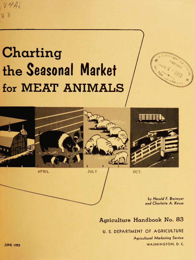
Charting the Seasonal Market for MEAT ANIMALS

by Harold F. Breimyer and Charlotte A. Kause

JUNE 1955

Agriculture Handbook No. 83

U. S. DEPARTMENT OF AGRICULTURE

Asricultural Marketins Service

WASHINGTON, D. C

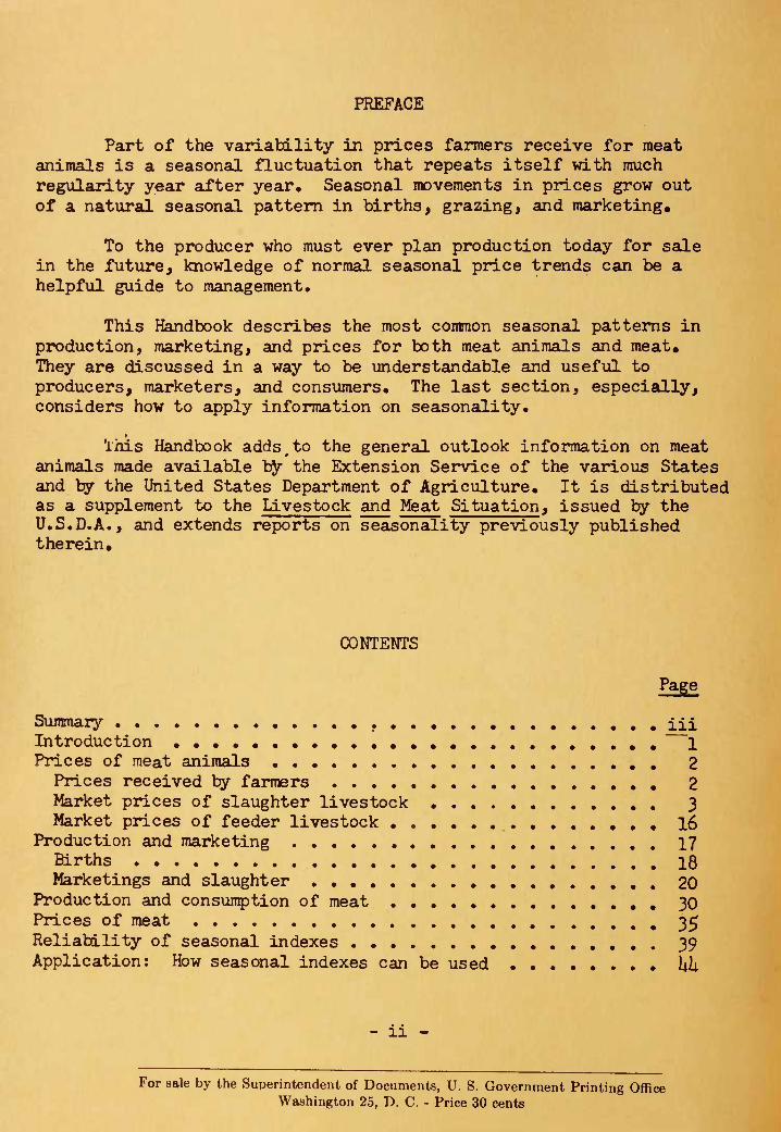
PREFACE

Part of the variabdlity in prices farmers receive for meat animals is a seasonal fluctuation that repeats itself vd.th much regularity year after year. Seasonal movements in prices grow out of a natural seasonal pattern in births, grazing, and marketing.

To the producer who must ever plan production today for sale in the future, knowledge of normal seasonal price trends can be a helpful guide to management.

This Handbook describes the most common seasonal patterns in production, marketing, and prices for both meat animals and meat. They are discussed in a way to be understandable and useful to producers, marketers, and consumers. The last section, especially, considers how to apply information on seasonality.

ïhis Handbook adds^to the general outlook information on meat animals made available l^ the Extension Service of the varioiis States and by the United States Department of Agriculture, It is distributed as a supplement to the Livestock and Meat Situation, issued by the U.S.D.A., and extends reports on seasonality previously published therein.

CONTENTS

• • Summary , lii Introduction • , 1 Prices of meat animals 2

Prices received by farmers 2 Market prices of slaughter livestock 3 Market prices of feeder livestock l6

Production and marketing 17 Births 18 Marketings and slaughter 20

Production and consumption of meat 30 Prices of meat 3^ Reliability of seasonal indexes , . 39 Application: How seasonal indexes can be used • kh

- 11 -

For sale by the Superintendent of Documents, U. S. Government Printing Office Washington 25, D. C. - Price 30 cents

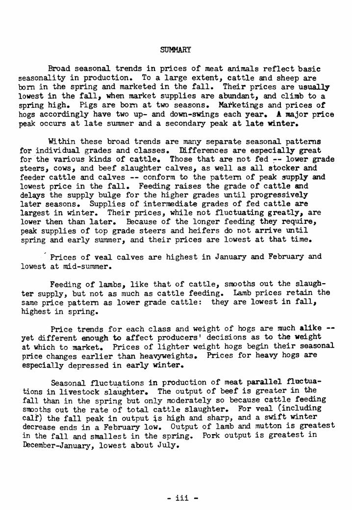
SUMMARY

Broad seasonal trends in prices of meat animals reflect basic seasonality in production. To a large extent, cattle and sheep are bom in the spring and marketed in the fall* Their prices are usually lowest in the fall, when market supplies are abundant, and climb to a spring high. Pigs are bom at two seasons. Marketings and prices of hogs accordingly have two up- and down-swings each year» A major price peak occurs at late summer and a secondary peak at late winter*

Within these broad trends are many separate seasonal patterns for individual grades and classes. Differences are especially great for the various kinds of cattle• Those that are not fed -- lower grade steers, cows, and beef slaughter calves, as well as all stocker and feeder cattle and calves — conform to the pattern of peak supply and lowest price in the fall. Feeding raises the grade of cattle and delays the supply bulge for the higher grades until progressively later seasons. Supplies of intermediate grades of fed cattle are largest in winter. Their prices, while not fluctuating greatly, are lower then than later. Because of the longer feeding they require, peak supplies of top grade steers and heifers do not arrive until spring and early summer, and their prices are lowest at that time.

Prices of veal calves are highest in January and February and lowest at mid-summer.

Feeding of lambs, like that of cattle, smooths out the slaughter supply, but not as much as cattle feeding. Lamb prices retain the same price pattern as lower grade cattle: they are lowest in fall, highest in spring.

Price trends for each class and weight of hogs are much alike — yet different enough to affect producers' decisions as to the weight at which to market. Prices of lighter weight hogs begin their seasonal price changes earlier than heavyweights. Prices for heavy hogs are especially depressed in early winter.

Seasonal fluctuations in production of meat parallel fluctuations in livestock slaughter* The output of beef is greater in the fall than in the spring but only moderately so because cattle feeding smooths out the rate of total cattle slaughter. For veal (including caljr) the fall peak in output is high and sharp, and a swift winter decrease ends in a February low. Output of lamb and mutton is greatest in the fall and smallest in the spring* Pork output is greatest in December-January, lowest about July.

- iii -

Total output of meat thus tends to be greatest in the fall and winter, and smallest in the summer. Storage of rather small quanti tie: of beef and somewhat more pork offsets part of the variation in supply, Also, consumer demand is a hit weaker in the hot summer months than at other times• Nevertheless, supplies of meat are larger, relative to demand, in winter than in summer. The result is a seasonal swing in prices of meat at retail. With some differences by meat and grade, prices average lowest in fall and winter and highest in spring and summer.

Seasonal patterns change over time as innovations are made in livestock production and marketing. Seasonal trends in prices of veal calves are markedly different in the 1950's than the 1920's because marketings have been affected by a shift from spring calving of milk cows to calving throughout the year. Hog producers have achieved earlier farrowing and faster raising and feeding. Seasonal swings in slaughter and prices of hogs therefore occur earlier than they once did. Increased use of home lockers and freezers has undoubtedly modified seasonal patterns in consumers' demand and consioraption of meat.

Indexes of seasonality are a good starting point for antici- pating the short-run future for prices of meat animals. But as average seasonal trends are seldom followed exactly in a given year, each producer needs to use other current information in arriving at his judgment of the economic outlook for his products at a particular time. Knowledge of the seasonal outlook can be applied in many ways. From it the producer can often adjust his production program so as to avoid low-price months; he can aim his marketing for the period promising best returns; and he can often recognize and take advantage of unusual rises and dips in the market that offer opportunity for profit.

- IV -

CHARTING THE SEASONAL MARKET FOR MEAT ANIMALS

By Harold F. Breinçrer and Charlotte A . Kause 1/

Statistical and Historical Research Branch Agricult\iral Economics Division

INTRODUCTION

A seasonal pattern marks the production and marketing of most kinds of livestock* Basically, spring is the season for births; Slimmer for pasturing; fall for marketing off grass; and fall and winter for feeding* Seasonal fluctuation appears in the number of livestock slaughtered and'in the flow of meat to consumers* The meat supply is usually largest in the fall and winter and smallest in the spring and summer* Prices of both meat animals and meats trace seasonal ups and downs, responding to seasonal variations in supplies and to some seasonal differences in demand*

So important and regular are these changes that it is helpful for livestock producers and others to know the most common or typical patterns* Tables and charts in this report present indexes of normal or average seasonal variation in prices, production, marketings and slaughter of live animals* Included also are indexes of seasonality in prices, production, consumption, and stocks of meat*

Indexes are computed from data as available back to 1921, except World War II years, but are adjusted for trend to apply primarily to years since the war (l9U7-53)# Many seasonal patterns have changed during the last 33 years, making an adjustment to postwar years essential* Indexes were derived by the ratio-to-moving average method* 2/ The indexes show, for each statistical measure, the normal value for each month as a percentage of the average for all months* An index of 131 for hog slaughter in January, for example, means that in an average year the number of hogs slaughtered in that month is 31 percent greater than the average for the entire 12 months* This reveals January as a month of relatively large slaughter.

1/ Part of the statistical work was contributed by the late Lucille W. Johnson, Statistical Assistant in the Statistical and Historical Research Branch* 2/ Procedure follows the form described in Foote, R. J., and

Fox, Karl A., Seasonal Variation: Methods of Measurement and Tests for Significance. U. S. Dept. Agr. Handbook U8, l6 pp.. Sept* 1952*

- 2 -

All the indexes are fomd in tables 1 to h. Most are plotted in accompanying charts (figures 1 to 29). Price indexes are plotted in simple line charts• Indexes of quantities marketed or produced are plotted in either line or strata charts• In some charts, several indexes are shown in their proportionate relation to each other by plotting all indexes on a single scale, with one of the grades or classes selected for the 100 percent line (fig. 2, for example). For these, seasonal values cannot be read directly from the chart but must be obtained from the table. Quantity relations are occasionally shown by strata in which the quantities of various grades or classes are presented cumulatively, so that they build up to a total (as in fig. 1$). The nature of the various charting devices will become clearer as each index is reviewed«

PRICES OF MEAT ANIMALS

Prices Received by Farmers

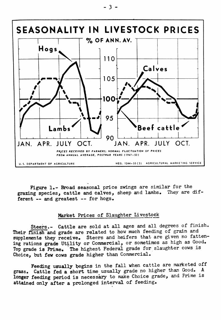
The broad sweep of seasonal trends in prices of meat animals may be seen in indexes for average prices received by farmers. For cattle, calves, sheep and lambs, the basic sequence of spring birth, summer grazing and fall marketing is reflected in a matching price pattern. Prices for these species are normally highest in the spring, lowest in the fall (table 1 and fig. l). ,For hogs, the pattern is different« Farmers raise two crops of pigs, one bom in the spring and a second in the fall« Marketings, not influenced by the grazing season, regularly occur 6 to 9 months after birth. Prices of hogs usually rise from late spring to a peak in late summer, then decline steadily for about 3 months. They are lowest in late fall and early winter. A small increase and small decrease usually take place during the winter and early spring when marketings of hogs from the fall pig crop are largest.

These are trends for average prices of all grades and classes of meat animals as sold« Of more interest to most producers of livestock is the seasonal behavior of individual grades and classes. A farmer preparing to sell a load of hogs or cattle wants to know, not a general average, but the most likely price trend for the particular kind of hogs or cattle he has for sale« Seasonal price patterns are by no means the same for every kind. Accordingly, seasonal trends in livestock prices are reported in more detail in the section that follows.

- 3 -

SEASONALITY IN LIVESTOCK PRICES

ives

JAN. APR. JULY OCT. JAN. APR. JULY OCT. PR¡CES RECEIVED BY FARMERS; NORMAL FLUCTUATION OF PRICES

FROM ANNUAL AVERAGE, POSTWAR YEARS (19áT-S3)

U. S. DEPARTMENT OF AGRICULTURE NEC. 1244-55(3) AGRICULTURAL MARKETING SERVICE

Figure !•- Broad seasonal price svdngs are similar for the grazing species, cattle and calves, sheep and lambs. They are different — and greatest — for hogs.

tfarket Prices of Slaughter Livestock

Steers.- Cattle are sold at all ages and all degrees of finish. Their finish and grade are related to how much feeding of grain and supplements they receive. Steers and heifers that are given no fatten- ing rations grade Utility or Commercial, or sometimes as high as Good. Top grade is Prime. The highest Federal grade for slaughter cows is Choice, but few cows grade higher than Commercial.

Feeding usually l?egins in the fall when cattle are marketed off grass. Cattle fed a short time usually grade no higher than Good. A longer feeding period is necessary to make Choice grade, and Prime is attained only after a prolonged interval of feeding.

- h

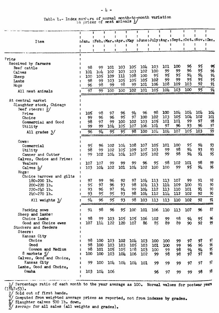
Tabl« l.- Index nun>.trs of normal month-to-month variation -jn prices of meat animals 1/

[ 1 t

Item ! •Jan. ■ •Feb.• •Mar,! ¡Apr.!

<

•May ¡Jtme. ¡July! ¡Aug.! ¡Sept.' ¡Oct.' ¡Nov. ¡Dec.

! Price ; Received by farmers :

Beef cattle : 98 99 101 103 105 lOU 103 101 100 96 95 95 Calves ! 101 lOU 102 103 103 102 100 99 99 96 9$ 96 Sheep : 100 105 109 111 108 100 95 95 95 9U 9h 9li Lambs 98 99 103 105 105 105 102 99 99 9S 95 95 Hogs ; 96 98 99 98 99 101 106 108 109 103 92 91

All meat animals ! 97 99 100 100 102 101 105 lOU 103 100 95 9k

At central market ! Slaughter stock, Chicago ;

Beef steers: 2/ : Prime ' 105 98 97 96 9U 96 98 100 loU loU lOl» 101«

Choice : 99 96 96 95 97 100 102 103 105 loU 102 101 Commercial and Good : • 98 97 99 100 102 103 105 101 101 99 97 98 Utility ! : 99 99 lOlt 105 107 106 101 97 96 93 96 97

All grades 3/ • 96 9U 9$ 95 98 100 loU lOU 107 105 103 99

Cows: Commercial ! 95 96 102 10Ü 108 107 105 101 100 95 9Í» 93 Utility : 98 99 102 105 109 107 103 99 98 9h 93 93 Canner and Cutter : 99 102 lOU loa 107 105 102 99 98 9U 91 95

Calves, Choice and Prime: Vealers ! 107 107 99 99 99 96 95 98 102 101 98 99 Calves k/ ! 103 lOU 102 101 lOU 102 100 100 99 95 9k 96

Hogs: Choice barrows and gilts ;

180-200 lb. ! 97 99 96 92 97 lOU 113 113 107 99 91 92 200-220 lb. ! 95 97 96 93 98 loU 113 llU 109 100 91 90 220-2U0 lb. : 93 96 97 9li 99 lOU 112 n3 110 101 91 90 2UO-270 lb. Í 93 95 95 93 98 loU 112 llU 112 102 92 90

All weights 3/ ! 9Ü 96 95 93 98 103 113 113 110 102 92 _91

Packing sows ! 91 98 96 95 100 101 106 110 113 107 96 87 Sheep and lambs:

Choice lambs 1 98 99 103 105 105 106 102 99 98 9U 95 96 Good and Choice ewes Í 107 111. 122 120 107 86 85 89 89 90 92 99

Stockers and feeders Steers :

Kansas City Choice ¡ ''. 98 100 103 102 loU 103 100 100 99 97 97 97 Qood ! 98 100 103 103 105 103 101 100 99 96 96 96 Common and Medium ! 98 101 105 105 108 103 100 99 98 9U 9U 95

8 markets ¿/ ! 100 100 103 lOU 106 102 99 98 98 97 97 96 Calves, Good and Choice,

Kansas City ! 99 100 lOU lOii loU 101 99 99 99 97 97 97 Lambs, Good and Choice,

Omaha \ 103 lOU 106 96 97 99 99 98 98

1/ Percentage ratio of each month to the year average as 100» Normal values for postwar years (19Íi7.53)- 2/ Sold out of first hands. 3/ Computed from weighted average prices as reported, not from indexes by grades« u/ Slaughter calves ÇOO lb. down» t/ Average for all sales (all weights and grades)♦

- 5 -

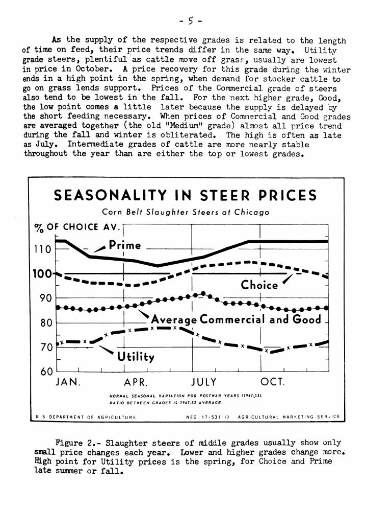
As the supply of the respective grades is related to the length of time on feed, their price trends differ in the same way. Utility grade steers, plentiful as cattle move off gras5:, usually are lowest in price in October* A price recovery for this grade during the winter ends in a high point in the spring, when demand for stocker cattle to go on grass lends support* Prices of the Commercial grade of steers also tend to be lowest in the fall* For the next higher grade. Good, the low point comes a little later because the supply is delayed by the short feeding necessary* Wlien prices of Comraercial and -Good grades are averaged together (the old "Medium" grade) almost all price trend during the fall and winter is obliterated* The high is often as late as July. Intermediate grades of cattle are more nearly stable throughout the year than are either the top or lowest grades*

SEASONALITY IN STEER PRICES Corn Beli Slaughter Steers at Chicago

%0F CHOICE AV

110

80

70 F

— Average Commercial and Good _ X MMM X

60

i^^X

Utility J L

JAN. APR. JULY OCT. NORMAL SEASONAL VARIATION FOR POSTWAR YEARS (1947-JS3).

RATIO BETWEEN GRADES IS 1947-53 AVERAGE

U S DEPARTMENT OF AGRICULTURE NEG 17-53(11) AGRICULTURAL MARKETING SERVICE

Figure 2*- Slaughter steers of middle grades usually show only small price changes each year» Lower and higher grades change more* High point for Utility prices is the spring, for Choice and Prime late summer or fall.

- 6 -

Prices for highly finished fed cattle that grade Choice and Prime follow a seasonal pattern opposite to that for Utility and Commercial» Price downtrends ordinarily mark the winter-early spring season when marketings of these upper grades increase* The low point for Choice steers and heifers usually comes sometime between late winter and mid-spring. Their prices then trend upward during the summei For Prime steers, peak marketings of which are last to appear because of the extra feeding required, price declines are latest of all* In an average year May is the month of lowest prices for the Prime grade, and recovery is slow until July-August* Prices of Choice and Prime steers and heifers are highest at late summer and early fall* Their supply is then seasonally smaller, while consumer demand for broiling meats, particularly steaks and ground beef, is strong at summer's end.

Indexes of normal seasonal trends in prices of steers by grades are given in table 1* The trends are also shown in figure 2* In the chart, all indexes are expressed in their relation to the year-long price of Choice steers* In this way the normal seasonal price patterns are accurately revealed both for each grade alone, and for relationships between grades. As a further explanation, in 19U7-53 prices of Utility steers at Chicago averaged 28 percent less than the price of Choice steers* Seasonal variations in Utility prices are therefore plotted in figure 2 vdth 72 percent as a base line (equivalent to 100 in the indexes of table 1)* In this way, average price relationships between Choice and Utility are preserved. The spreads of 19 percent between the two grades in April and 37 percent in October, as read approximately from the chart, are reliable observations of varying spreads between grades in an average year* The charting device adopted in figure 2 is used in several other charts also*

Cows*- Seasonal trends in prices of slaughter cows are fairly consistent year to year and are similar for all grades* They conform to the seasonality in prices of lower grade cattle* Mid-fall, the end of the grazing season, finds suprlies largest and prices lowest. In early spring, when grazing begins in most regions, stocker demand is strong and prices of cows move up to their yearly peak (table 1 and fig* 3)»

In a normal year, prices of Canner and Cutter cows reach their low point earlier and recover faster than do prices of the Utility and Commercial grades* By January, the Canner and Cutter grade is up 8 percentage points from its low while the Utility grade usually advances only S points and Commercial, 2 points. In all other respects, seasonal price trends for the several grades of slaughter COVÍS are essentially the same*

- 7 -

SEASONALITY IN COW PRICES Slaughfer Cows at Chicago

% OF UTILITY AV.T ^ >■ '

120

100

Commercial

"TWi

-• • • ♦

80

60

Canner & Cutter

JAN. APR JULY OCT NORMAL SEASONAL VARIATION FOR POSTWAR YEARS ( I9<7- S3). RATIO BETWEEN GRADES IS 1947-53 AVERAGE.

U, S. DEPARTMENT OF AGRICULTURE NEC. 811-54(5) AGRICULTURAL MARKETING SERVICE

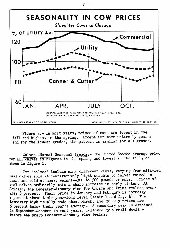
Figure 3.- In most years, prices of cows are lowest in the fall and highest in the spring. Except for more uptiim by year's end for the lowest grades, the pattern is similar for all grades.

Calves—Normal Seasonal Trends.- The United States average price for all calves is highest in the spring and lowest in the fall, as shown in figure 1,

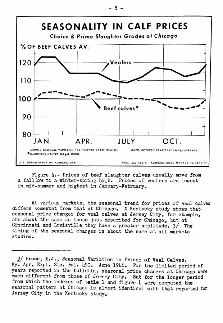
But "calves'» include many different kinds, varying from milk-fed veal calves sold at comparatively light weights to calves raised on grass and sold at heavy weight—300 to 500 pounds or more. Prices of veal calves ordinarily make a sharp increase in early winter. At Chicago, the December-January rise for Choice and Prime vealers aver- ages 8 percent. Their price in January and February is normally 7 percent above their year-long level (table 1 and fig. U). The tenqporary high usually ends about March, and by July prices are 5 percent below their year's average. A secondary peak is attained in September-October in most years, followed by a small decline before the sharp December-January rise begins.

- 8 -

SEASONALITY IN CALF PRICES Choice & Prime Slaughfer Grades at Chicago

%OF BEEF CALVES AV.

120

110

100

90

80

■v—r— ^ Beef calves* ^, y_

1 JAN APR JULY OCT.

NORMAL SEASONAL VARIATION FOR POSTWAR YEARS (1947-53).

^SLAUGHTER CALVES 500 j-B. DOWN.


RAT/0 BETWEEN CLASSES IS 1947-53 AVERAGE.

NEC. 1256-54(12) AGRICULTURAL MARKETING SERVICE

Figure li.- Prices of beef slaughter calves usually move from a falllow to a winter-spring high. Prices of vealers are lowest in mid-summer and highest in January-February.

At various markets, the seasonal trend for prices of veal calves differs somewhat from that at Chicago♦ A Kentucky stuc^ shows that seasonal price changes for veal calves at Jersey City, for example, are about the same as those just described for Chicago, but at Cincinnati and Louisville they have a greater amplitude. 3/ The timing of the seasonal changes is about the same at all markets studied.

3/ Erown, A.J., Seasonal Variation in Prices of Veal Calves. Ky. Agr. Expt. Sta. Bui. ];90^ June 19U6. For the limited period of years reported in the bulletin, seasonal price changes at Chicago were much different from those of Jersey City. But for the longer period from which the indexes of table 1 and figure h were computed the seasonal pattern at Chicago is almost identical with that reported for Jersey City in the Kentucky study.

- 9 -

Prices of the heavier slaughter calves iollow a seasonal pattern resembling that for cows and lower grade steers* Unlike prices of veal calves, which are high in January-February but otherwise fairly stable, prices of heavy slaughter calves undergo their greatest changes in the fall when they dip to a low as marketings increase. Their December- January upturn is moderate and prices are relatively steady through all other months. The high price period for heavy slaughter calves extends over a long span from January to June (fig. !;)•

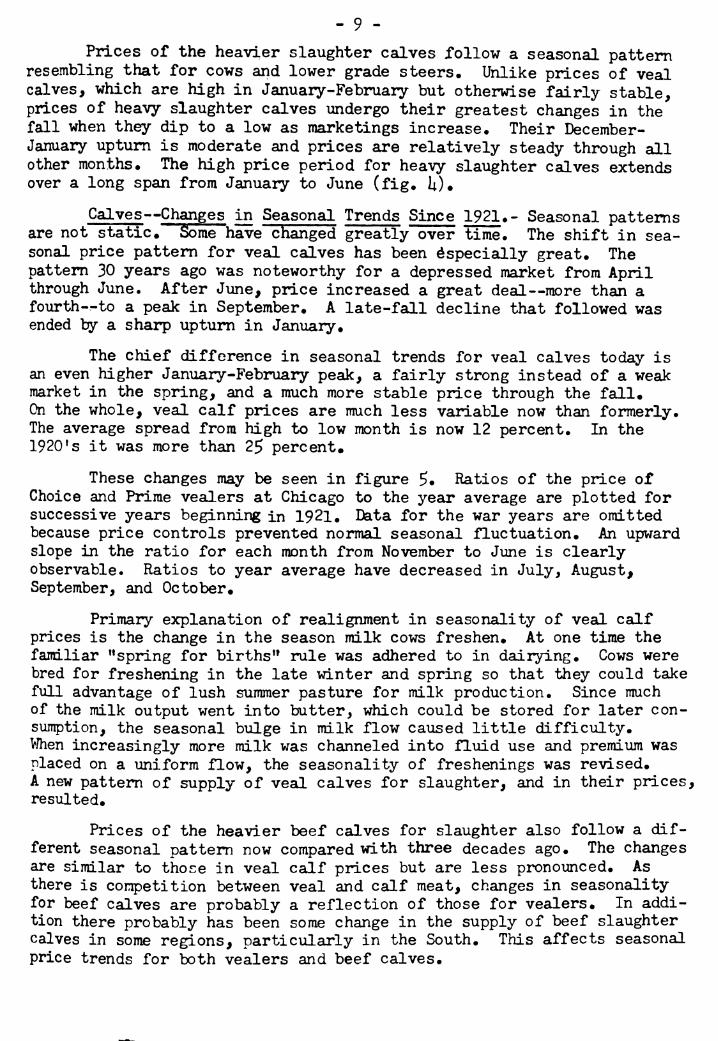
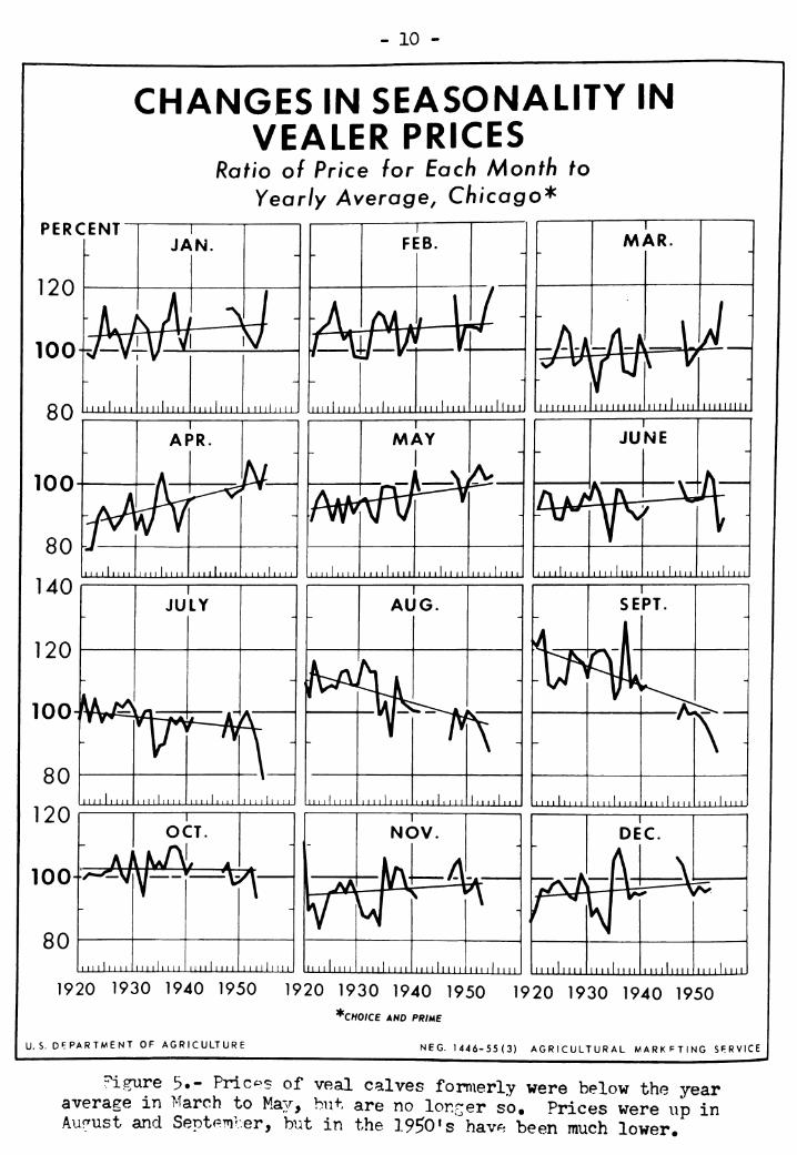
Calves—Changes in Seasonal Trends Since 1921.> Seasonal patterns are not static. Some have changed greatly over time. The shift in seasonal price pattern for veal calves has been especially great. The pattern 30 years ago was noteworthy for a depressed market from April through June. After June, price increased a great deal—more than a fourth—to a peak in September. A late-fall decline that followed was ended by a sharp upturn in January.

The chief difference in seasonal trends for veal calves today is an even higher January-February peak, a fairly strong instead of a weak market in the spring, and a much more stable price through the fall. On the whole, veal calf prices are much less variable now than formerly. The average spread from high to low month is now 12 percent. In the 1920*s it was more than 2$ percent«

These changes may be seen in figure 5» Ratios of the price of Choice and Prime vealers at Chicago to the year average are plotted for successive years beginning in 1921. Data for the war years are omitted because price controls prevented normal seasonal fluctuation. An upward slope in the ratio for each month from November to June is clearly observable. Ratios to year average have decreased in July, August, September, and October.

Primary explanation of realignment in seasonality of veal calf prices is the change in the season milk cows freshen. At one time the familiar "spring for births" rule was adhered to in dairying. Cows were bred for freshening in the late winter and spring so that they could take full advantage of lush summer pasture for milk production. Since much of the milk output went into butter, which could be stored for later consumption, the seasonal bulge in milk flow caused little difficulty. V/hen increasingly more milk was channeled into fluid use and premium was placed on a uniform flow, the seasonality of freshenings was revised. A new pattern of supply of veal calves for slaughter, and in their prices, resulted.

Prices of the heavier beef calves for slaughter also follow a different seasonal pattern now compared with three decades ago. The changes are similar to those in veal calf prices but are less pronounced. As there is competition between veal and calf meat, changes in seasonality for beef calves are probably a reflection of those for vealers. In addition there probably has been some change in the supply of beef slaughter calves in some regions, particularly in the South. This affects seasonal price trends for both vealers and beef calves.

- 10 -

CHANGES IN SEASONALITY IN VEALER PRICES

Ratio of Price for Each Month to Yearly Average, Chicago*

PERCENT

120

100 v-v^

FEB.

éèé^ QQ ltml»ii ■iMiiliiM liiiilimli iiilnii I li 111 I 11111 i i 11 ■ i 111 li 11111111 ' 11111111 ll 11 11 í 11 111 M IIII M I ll 11ÍI I III11 11111 IN I

100

MAY

N^^H^ " I I ll M I ll I II ll I M ll II lllllll I I I ll I I I I I 111 II I 11 I I I I I 1 I I 11 nil II I ll I I I ll I I 1 1 I I III ll I I ill I I ll ll II I lilll II II I II II I I I III I 11 1

JUNE

""^^Wii

100

1920 1930 1940 1950 1920 1930 1940 1950 1920 1930 1940 1950

*CHOICE AND PRme

NEC. 1446-55(3) AGRICULTURAL MARKETING SERVICE U.S. DEPARTMENT OF AGRICULTURE

Figure 3.- Pric^^s of veal calves formerly were below the year average in March to May, but are no longer so. Prices were up in Aur'ust and Septem-ver, but in the 1950's hav*i been much lower.

- 11 -

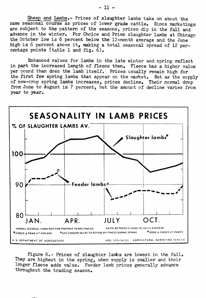
Sheep and Lambs•- Prices of slaiaghter lambs take on about the same seasonal coiirse as prices of lower grade cattle. Since marketings are subject to the pattern of the seasons, prices dip in the fall and advance in the viinter* For Choice and Prime slaughter lambs at Chicago the October low is 6 percent below the 12-month average and the June high is 6 percent above it, making a total seasonal spread of 12 percentage points (table 1 and fig» 6).

Enhanced values for lambs in the late winter and spring reflect in part the increased length of fleece then. Fleece has a higher value per pound than does the lamb itself* Prices usually remain high for the first few spring lambs that appear on the market* But as the supply of new-crop spring lambs increases, prices decline. Their normal drop from June to August is 7 percent, but the amount of decline varies from year to year.

SEASONALITY IN LAMB PRICES % OF SLAUGHTER LAMBS AV.

100

90

80

Slaughter lambs

Feeder lambs^

\--"

JAN. APR JULY OCT. NORMAL SEASONAL VARIATION FOR POSTWAR YEARS (1947-53) RATIO BETWEEN CLASSES IS 1947-53 AVERAGE

* CHOICE & PRIME AT CHICAGO ^NOT ENOUGH SALES TO ESTABLISH PRICES DURING SPRING ^GOOD ¿ CHOICE A T OMAHA


Figure 6.- Prices of slaughter lambs are lowest in the fall« They are highest in the spring, when supply is smaller and their longer fleece adds value• Feeder lamb prices generally advance throughout the trading season*

. 12 -

Prices of slaughter ewes fluctuate much more during each year than do lamb prices. The mid-summer low (just after shearing) is 15 percent less than the year's average* In March, prices are normally 22 percent above the yearns level (table 1; not charted).

Prices of sheep and lambs have held about the same seasonal course for many years. But prices in December-March, the marketing period for fed lambs, now show a little less seasonal rise than they did in earlier years. Summertime prices are a little higher relative to the year's average level than they once were. But in the last few years, June prices have tended to drift lower, probably because many producers have successfully striven to sell spring lambs on the attractive early- season market, while others have marketed proportionately more wheat field lambs late, after a turn in the feedlot.

SEASONALITY IN PRICES OF LIGHT AND HEAVY HOGS

7o OF 240-270 LB. AV.

no

100

70

200-220 lb. barrows and gilts

JAN APR JULY OCT. CHICAGO PRICES. NORMAL SEASONAL VARIATION FOR POSTWAR YEARS (1947-53).

RATIO BETWEEN WEIGHTS AND CLASSES IS 1947-53 AVERAGE *ALL WEIGHTS


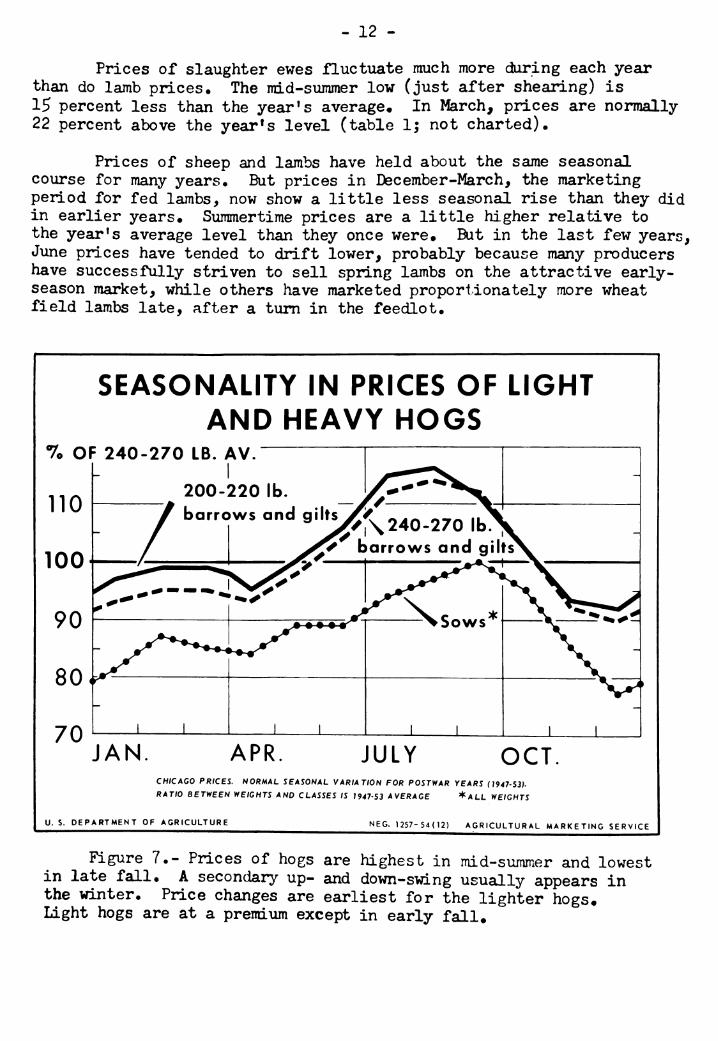
Figure 7.- Prices of hogs are highest in mid-summer and lowest in late fall* A secondary up- and down-swing usually appears in the winter* Price changes are earliest for the lighter hogs* Light hogs are at a preirdxim except in early fall*

- 13 -

Hogs—Normal Seasonal Trends*- The basic seasonal!ty for all kinds of hogs is the sanie: prices are highest of the year in mid- to late-summer, then decline greatly during the fall. After touching a low in late fall or early winter they rise to a secondary peak about late winter* They then decline briefly before a very substantial summer advance commences (fig* 7).

Prices are highest in mid-summer because fewer hogs are available for slaughter then* Low prices in December result from peak marketings at that time*

Two price peaks and two declines each year are a simple reflection of the two pig crops. Because the fall crop is the smaller of the two, price fluctuations in the winter and spring, when hogs therefrom are marketed, are less severe than those in the summer and fall* Price increases in the summer would be even more extreme except for the substantial number of sows sold for slaughter then*

Although the seasonal price paths are similar for all weights of hogs, they are not identical* To a large extent, the patterns follow each other successively for the progressively heavier weights. Price changes come first for the lightest hogs* They are slightly later for medium weight hogs; delayed still more for heavy hogs; and latest of all for the heaviest barrows and for sows (figs. 7 and 8). Prices of lightweight barrows and gilts, in a normal year, nearly hit their peak by July and by early fall are declining fast* Prices of heavy barrows hold high longer and usually do not break sharply until October. Prices of sows are even slower to attain their year's top level. Prices of all heavy hogs drop even faster than light hogs in late fall and by December are much below those of the lighter weights. Heavy barrows remain sharply discounted during the winter; their total seasonal gain in that season is rather small. Prices of sows, however, rise a good deal from their usual early December low. Demand for sows for spring farrowing restricts the supply for slaughter during the winter*

Reason for the delayed price movement for progressively heavier hogs is the same as for the progressively higher grade steers -- the more time required for feeding them makes marketings and attendant price changes naturally appear later*

Hogs—Changes in Seasonal Trends Since 1930^- In the price of hogs, as in that of calves, seasonal patterns have changed considerably. It will be noted later that seasonal variations in hog production and marketing are being measurably reduced. Figure 9 shows price trends also are different now from those in earlier years*

In figure 9, ratios of the hog prices for each month to the year average are plotted for years since 1930 except war years* Data are for medium weight (220-2liO pound) barrows and gilts at Chicago*

- lU -

SEASONALITY IN BARROW AND GILT PRICES, BY WEIGHT GROUPS

7o OF ANN. AV.

JAN. APR. JULY OCT. CHICAGO PRICES; NORMAL FOR POSTWAR YEARS (1947-53)

U. S. DEPARTMENT OF AGRICULTURE N EG. 679 - 54 (4) AGRICULTURAL MARKETING SERVICE

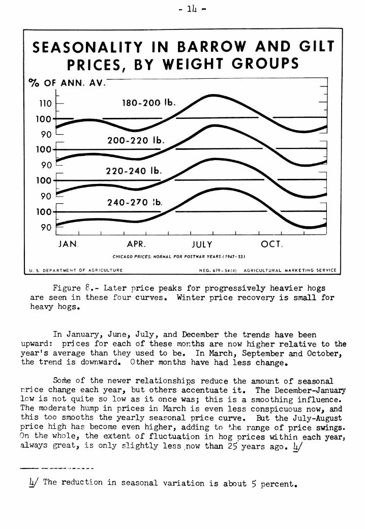
Figure 8." Later price peaks for progressively heavier hogs are seen in these four curves • Winter price recovery is small for heavy hogs#

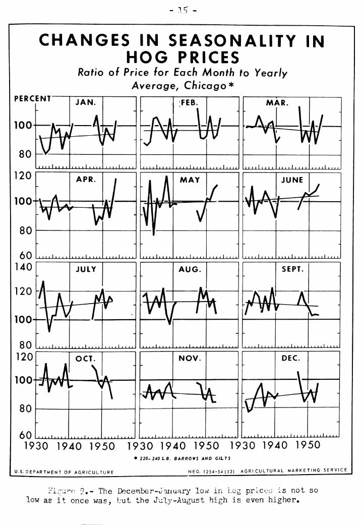
In January, June, July, and December the trends have been upward: prices for each of these months are now higher relative to the yearns average than they used to he. In March, September and October, the trend is downward. Other months have had less change.

Some of the newer relationships reduce the amount of seasonal rrice change each year, but others accentuate it. The December-January low is not quite so low as it once was; this is a smoothing influence. The moderate hujnp in prices in March is even less conspicuous now, and this too smooths the yearly seasonal price curve. But the July-August price high has become even higher, adding to the range of price swings. On the whole, the extent of fluctuation in hog prices within each year, always great, is only slightly less now than 25 years ago. U/

k/ The reduction in seasonal variation is about 5 percent.

- ÎÇ -

CHANGES IN SEASONALITY IN HOG PRICES

Ratio of Price for Each Month to Yearly Average, Chicago*

PERCENT

100

1930 1940 1950 1930 1940 1950 1930 1940 1950 * 220-240 LB. BARROY/S AND GILTS

U.S.DEPARTMENT OF AGRICULTURE NEC. 1254-54 (12) AGRICULTURAL MARKETING SERVICE

Vlr.i'^c' 9.- The Dec ember-January low in Log price:; Is not so low as it once was, but the July-August high is even higher*

. 16 -

Changes in seasonal!ty of hog prices are chiefly attributed to corresponding changes in production* Farrowings are earlier and pigs are raised and fed faster. Marketings accordingly are a bit earlier in the calendar year. These changes are reviewed in more detail in a later section. The higher July-August price peak has other origins: there is evidence that slaughter of sov/s adds relatively less to barrow and gilt slaughter than in former years, owing to the increased number of sows retained for fall farrowing. Movement of population from farm to city and growing use of refrigerated food storage in homes have lifted summer demand for pork.

Market Prices of Feeder Livestock

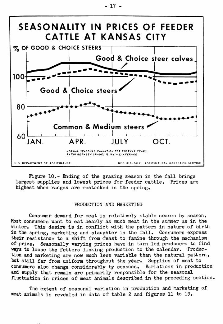
Prices of feeder livestock are even more closely associated ivith the grazing season than are prices of slaughter stock. Prices are low in the fall when herds must be reduced as the grazing season ends. They are higher in the spring when greening of the grass brings a need for restocking.

Only in small detail are seasonal price trends different for various kinds of feeder stock. Indexes for Choice feeder steers at Kansas City vary betvxeen a low of 97 in the fall and a high of lOk in May, Lower grades fluctuate more widely; for Comnon and Medium the range is from 9U to 108 percent, in a normal year (table 1 and fig. 10),

Prices for Good and Choice feeder steer calves reach their high earlier than do steers, and their overall fluctuation throughout a year is rather small.

The marketing season for feeder lambs is largely confined to the fall and winter. Price quotations at other times are often nominal. Prices are low when first shipments begin in late summer. They increase only a little until the end of the year. By January, however, a substantial advance is ordinarily registered. The normal top is at the season's end in mid- to late winter (table 1 and fig. 6),

No seasonal index has been computed for prices of feeder pigs# Many feeder pigs are bought and sold in Minnesota and neighboring States but trade elsewhere is rather small.

- 17 -

SEASONALITY IN PRICES OF FEEDER CATTLE AT KANSAS CITY

% OF GOOD & CHOICE STEERS

100

Good & Choice steer calves /

Good & Choice steers

60

-•-•-

Common & Medium steers J L J L J L

JAN APR JULY OCT. NORMAL SEASONAL VAHIATION FOR POSTWAR YEARS. RATIO BETWEEN GRADES IS 1947-53 AVERAGE.


Figure 10.- Ending of the grazing season in the fall brings largest supplies and lowest prices for feeder cattle. Prices are highest when ranges are restocked in the spring.

PRODUCTION AND MARKETING

Consumer demand for meat is relatively stable season by season. Most consumers want to eat nearly as much meat in the summer as in the winter. This desire is in conflict with the pattern in nature of birth in the spring, marketing and slaughter in the fall. Consumers express their resistance to a shift from feast to famine through the mechanism of price. Seasonally varying prices have in turn led producers to find ways to loose the fetters linking production to the calendar. Produc- tion and marketing are now much less variable than the natural pattern, but still far from uniform throughout the year. Supplies of meat to consumers also change considerably by seasons. Variations in production and supply that remain are primarily responsible for the seasonal fluctuation in prices of meat animals described in the preceding section.

The extent of seasonal variation in production and marketing of nieat animals is revealed in data of table 2 and figures 11 to 19•

- 18 -

Births

More lambs are bom in the spring than at any other season^ Calves of beef breeding also are usually bom in the spring* To this extent, the natural seasonal pattern has been preserved* In parts of the Southivest, the Pacific Coast, and some other areas, however, a very considerable number of lambs and beef calves are bom in fall and TO-nter*

Not long ago most dairy calves also were bom in the late winter and sprn\ng. Producers now schedule more dairy cows for fall freshening. A 195U report shows that in Minnesota, peak freshening months are now October and November* Each of the two months accounts for l5 percent of the year's total number of freshenings* In the h months September to December, Sh percent of the total occurs* 5/

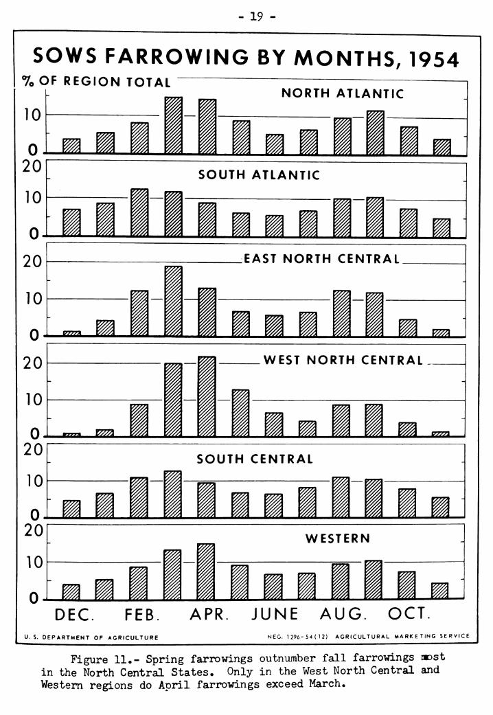
Except for the figures in the Minnesota study, we have few data on births of lambs and calves ty months* Data for hogs, on the other hand, have been reported for many years* Typically, pigs are bom in two pig crops* "Spring'* farro^ri.ngs, centering in March and April, outnumber farrowings in the "fall," in which August and September are the biggest months* But monthly differences in farrowings have been reduced as the fall crop has become larger relative to the spring crop and as more sows have farrowed in mid-winter and mid-summer* Also, farrowings have generally been moved to earlier months in each season*

Figure 11 portrays the distribution of farrowings by months in 195Ü by regions* Farrowings are latest in the West North Central and Western regions, the only ones where more sows farrow in April than in I4arch* Farrowings in the West North Central region are highly concentrated in March, April, and May* In the warmer South, a sizable number of sows farrow as early as Januarj»- and February, and the monthly pattern is relatively smooth* 6/

In the 1920's, two-thirds of all pigs were bom in the spring crop CDecember-^!ay), which thus was twice as large as the fall crop* In the 1950^s, the ratio between the two crops has been reduced to 60:L;0. A rising proportion of fall pigs is due not only to the universal trend toward two litters each year (which make fullest use of facilities), but also to declining importance of the traditional one-crop States* Nebraska and the Dakotas, for example, where even now 3/ii to 7/8 of all pigs are spring pigs, raised almost 15 percent of the United States total pig crop in the 1920's• but only 8 percent in 1950-5;U-

5/ From special release dated Sept* 22, 195U from Div. of Admin* Serv*, Dairy and Food, Minn* Dept. Agr., St* Paul, Minn., and Agr* Mktg. Service, U* S. Dept. Agr*

6/ See Kause, Charlotte, Regional Differences in Season of Farrowing. The Livestock and Meat Situation* Agr* Mktg* Service, U* S* Dept* Agr. Jan. 7, 1955, P^ iT.

- 19 -

SOWS FARROWING BY MONTHS, 1954 7o OF REGION TOTAL

10

0 20

10

Q.

20

10

ÉJ á

NORTH ATLANTIC

m

SOUTH ATLANTIC

Ü rz

WLML EAST NORTH CENTRAL

LI ^ ^ ^^

20

10

0. 20

10

0. 20

10

.^^

—^ WEST NORTH CENTRAL

i^ZL

SOUTH CENTRAL

^

i É WA

i JLM

^ ^ ^

WESTERN

T7y

DEC. FEB. APR. JUNE AUG. OCT. U.S. DEPARTMENT OF AGRICULTURE NEG. 1296-54(12) AGRICULTURAL MARKETING SERVICE

Figure !!•- Spring farrowings outnumber fall farrowings nost in the North Central States* Only in the West North Central and Western regions do April farrowings exceed March.

. 20 -

By making use of electricity, new eqxiipment, and improved practices, hog producers have learned to produce more pigs in the cold of mid-winter and the heat of mid-sumraer* The change has advanced the average date of farrowings of both spring and fall crops; and it has smoothed out monthly differences in farrowings* In 1930-3U, only 17 percent of all spring sows farrowed before March Ij in 1951|.^ 27 percent farrowed before that date* Similarly, in 1930-3li J)me-August farrowings were Ul percent of the fall total, but in 1951| summer litters were up to 55 percent* Between 1930-3U and 195U the extent of variation in farrowings between months was reduced a fourth*. 7/ Furthermore, in at least some States the size of litters saved has been increased sub- stantially in winter and summer months* Therefore, the number of pigs saved has shown even more change toward early date and reduced month- to-month variation than has the number of sows farrowed* 8/

Marketings and Slaughter

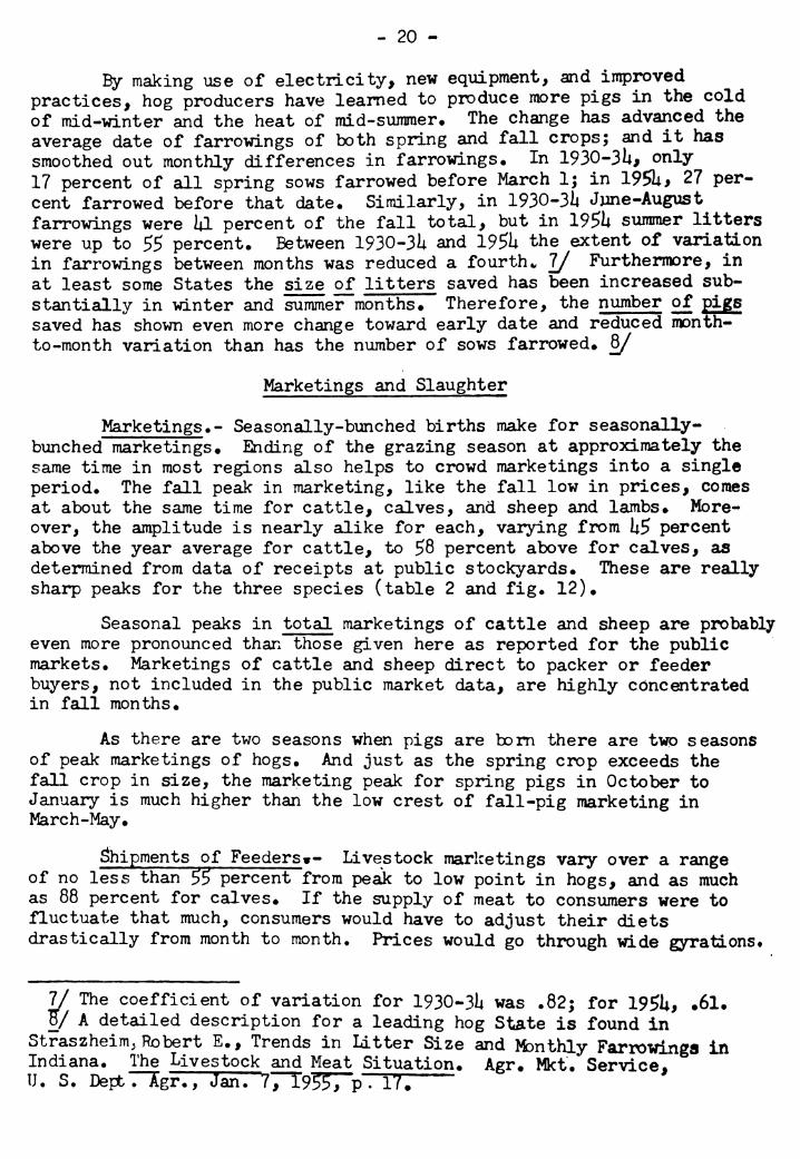
Marketings*- Seasonally-bunched births make for seasonally- bunched marketings* Ending of the grazing season at approximately the same time in most regions also helps to crowd marketings into a single period* The fall peak in marketing, like the fall low in prices, comes at about the same time for cattle, calves, and sheep and lambs* More- over, the amplitude is nearly alike for each, varying from U5 percent above the year average for cattle, to 58 percent above for calves, as determined from data of receipts at public stockyards* These are really sharp peaks for the three species (table 2 and fig* 12)*

Seasonal peaks in total marketings of cattle and sheep are probably even more pronounced than those given here as reported for the public markets* Marketings of cattle and sheep direct to packer or feeder buyers, not included in the public market data, are highly concentrated in fall months*

As there are two seasons when pigs are bom there are two seasons of peak marketings of hogs* And just as the spring crop exceeds the fall crop in size, the marketing peak for spring pigs in October to January is much higher than the low crest of fall-pig marketing in March-May*

¡Shipments of Feeders^- Livestock marketings vary over a range of no less than 55 percent from peaJc to low point in hogs, and as much as 88 percent for calves* If the supply of meat to consumers were to fluctuate that much, consumers would have to adjust their diets drastically from month to month* Prices would go through wide gyrationst

7/ The coefficient of variation for 1930-314 was .82; for 195U, .61* ÏÏ/ A detailed description for a leading hog State is found in

Straszheim^ Robert E*, Trends in Litter Size and Monthly Fariowinga in Indiana. The Livestock and Meat Situation* Agr. Mkt* Service, U. S. DepbTTgr., Jan. 77^9^^pTTr;

- 21 -

SEASONALITY IN LIVESTOCK MARKETINGS*

JAN. APR. JULY OCT. JAN. APR. JULY OCT. NORMAL SEASONAL VARIATION FOR POSTWAR YEARS (»947-53) *TOTAL RECEIPTS AT PUBLIC STOCKYARDS

U.S. DEPARTMENT OF AGRICULTURE NEC. 1451-55; 1) AGRICULTURAL MARKETING SERVICE

Figure 12.- Marketings are highly concentrated at the end of the grazing season for all meat animals except hogs, A November- January high in hog marketings reflects large I'iarch-April

farrowings.

The seasonal meat supply, to be sure, is not so variable as the oscillations in livestock marketings would indicate. Prime stabilizer for pork is the extensive storage of dressed pork and processed pork products. For other meats, it is feedlot feeding.

Hogs are not adaoted to extended feeding beyond a preferred market weight. At heavy weights their grade and price are reduced. Cattle and lambs, on the other hand, are of satisfactory flesh for slaughter at a rather wide range of age and weight; adding extra weight and finish increases their worth. Consequently, specialized feedlot feeding of lambs and cattle plays an economic role not

feasible for hogs. 9/

9/ In some areas, chiefly the northern Com Belt, a substantial trade e:dsts in feeder pigs, sold before they reach slaughter weight for additional feeding by the buyer.

- 22 -

Cattle & calves

300

200 100

0

sheep & lambs

-V

SEASONALITY IN FEEDER SHIPMENTS Receipts in 8 Corn Belt States

%OF ANN. AV."

300

200

100

0

JAN APR JULY OCT


NORMAL SEASONAL VARIATION FOR POSTÂ^ YEARS Í J947-53)

NEC. 1450-55(1) AGRICULTURAL MARKETING SERVICE

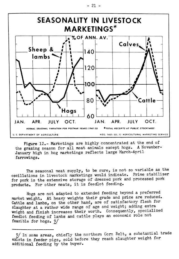
Figure 13 •- More than half of yearly movement of feeder cattle and lambs to the Com Belt takes place in a few fall months*

Both cattle and lambs are put on feed in greatest number at the end of the grazing season* Slightly more than half of all inshipments of feeder cattle to the Com Belt arrive in the 3 months September to November (fig* 13)• Seasonal timing of feeder cattle movement is somewhat different in the West, particularly in California*

A wide selection of programs is open to cattle feeders* Low grade cattle may be given a quick feed of 30 to 60 days* Heavy cattle can be topped off by a similar short feed* At the other extreme, steer calves are fed as long as 12 to lli months for sale at Prime grade« Seasonally-concentrated marketings of grass cattle are thereby trans- formed into a more evenly distributed supply of slaughter cattle of higher grade and weight«

- 23 -

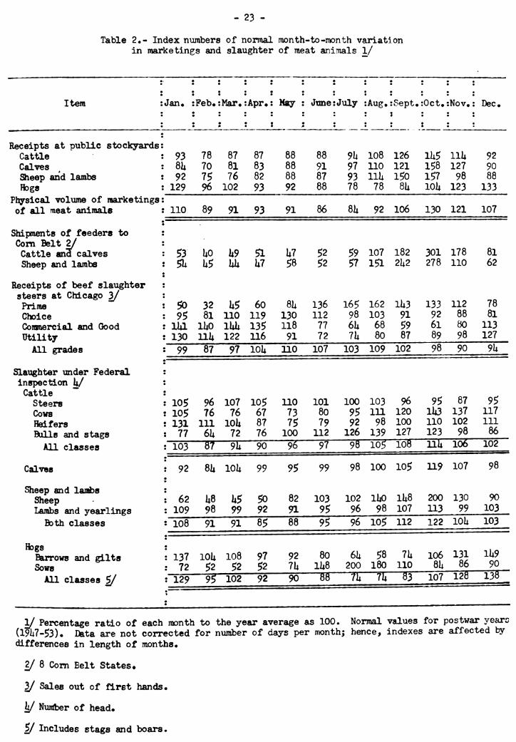
Table 2«- Index numbers of normal month-to-month variation in marketings and slaughter of meat animals 1/

Item : Jan. ¡Feb.- ÍMar.* Apr.' \ May !

1

: June' ¡July :Aug, rSept.:

•

Oct.' •Nov. ! ! Dec.

Receipts at public stockyards: CatUe : 93 78 87 87 88 88 9li 108 126 1U5 IIU 92 Calves : 8U 70 81 83 88 91 97 110 121 158 127 90 Sheep and lambs : 92 75 76 82 88 87 93 llU 150 157 98 88 Hogs : 129 96 102 93 92 88 78 78 8U loU 123 133

Phgrsical volume of marketings: of all meat animals : 110 89 91 93 91 86 8U 92 106 130 121 107

Shipments of feeders to : Com Belt 2/ Cattle ana calves 53 UO 1J9 51 U7 52 59 107 182 301 178 81 Sheep and lambs : Î 5U U5 Uli U7 58 52 57 151 2U2 278 110 62

Receipts of beef slaughter steers at Chicago 3/ Prime ! 5Ö 32 U5 60 8U 136 165 162 1U3 133 112 78 Choice ! 95 81 110 119 130 112 98 103 91 92 88 81 Commercial and Good ! lia lUO lUU 135 118 77 6U 68 59 61 Ö0 113 utility ! 130 llU 122 116 91 72 7U 80 87 89 98 127 All grades : 99 87 97 loU 110 107 103 109 102 98 90 9U

Slaughter under Federal inspection U/ Cattle Steers : 10Ç 96 107 105 110 101 100 103 96 95 87 95 Cows : 10Ç 76 76 67 73 80 95 111 120 11*3 137 117 Heifers : 131 111 lOU 87 75 79 92 98 100 110 102 111 Bulls and stags : 77 6U 72 76 100 112 126 139 127 123 98 86

All classes : 103 8? 91* 90 96 97 98 io5 108 111* 106 102

Calves i 92 8U lOU 99 95 99 98 100 105 119 107 98

Sheep and lambs Sheep : 62 U8 U5 50 82 103 102 lUo 11*8 200 13Ü 90 Lambs and yearlings : 109 98 99 92 91 95 96 98 107 113 99 103

Both classes : 108 91 91 85 88 95 96 105 112 122 lOl* 103

Hogs Barrows and gilts i 137 lOU 108 97 92 80 6U 58 7U 106 131 1U9 Sows : 72 52 52 52

92 7U 90

1U8 ■ 88

200

71* 1Ö0

71*

110 ÖU 86 90

All classes S/ : 129 9^ 102 83 107 120 138 • " •

1/ Percentage ratio of each month to the year average as 100. Normal values for postwar years (19li7-53)» Data are not corrected for number of days per month; hence, indexes are affected by differences in length of months.

2/ 8 Com Belt States*

3/ Sales out of first hands.

y Nuitíber of head.

y Includes stags and boars.

- 2ii -

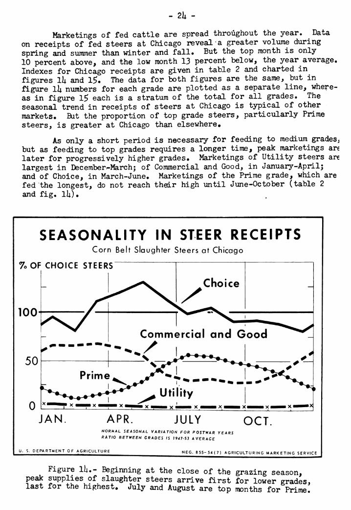
Marketings of fed cattle are spread throughout the year. Data on receipts of fed steers at Chicago reveal a greater volume during spring and summer than winter and fall. But the top month is only 10 percent above, and the low month 13 percent below, the year average. Indexes for Chicago receipts are given in table 2 and charted in figures lu and 15. The data for both figures are the same, but in figure Ik numbers for each grade are plotted as a separate line, where- as in figure 15 each is a stratum of the total for all grades. The seasonal trend in receipts of steers at Chicago is typical of other markets. But the proportion of top grade steers, particularly Prime steers, is greater at Chicago than elsewhere.

As only a short period is necessary for feeding to mediiim gradesj but as feeding to top grades requires a longer time, peak marketings are later for progressively higher grades. Marketings of Utility steers are largest in December-Marchj of Commercial and Good, in January-Aprilj and of Choice, in March-J\ine. Marketings of the Prime grade, which are fed the longest, do not reach their high until J\me-October (table 2 and fig. lU).

SEASONALITY IN STEER RECEIPTS Corn Belt Slaughter Steers at Chicago

7o OF CHOICE STEERS

100

Commercial and Good

JAN APR JULY OCT. NORMAL SEASONAL VARIATION FOR POSTWAR YEARS

RATIO BETWEEN GRADES IS 1947-53 AVERAGE

U. S. DEPARTMENT OF AGRICULTURE NEC. 855-54(7) AGRICULTU RIN G MARKETING SERVICE

Figure li;.- Beginning at the close of the grazing season, peak supplies of slaughter steers arrive first for lower grades, last for the highest. July and August are top months for Prime.

- 25

SEASONALITY IN STEER RECEIPTS Corn Belt Slaughter Steers at Chicago

%0F TOTAL STEERS AV.

120

100 UTILITY

—^Total receipts-

JAN APR JULY OCT NORMAL SEASONAL VARIATION FOR POSTWAR Y EARS ( 1947 - 53 )

RELATIONSHIPS BETWEEN GRADES ARE 1947-53 AVERAGE

U. S. DEPARTMENT OF AGRICULTlÊ NEC. 1449-55(1) AGRICULTURAL MARKETING SERVICE

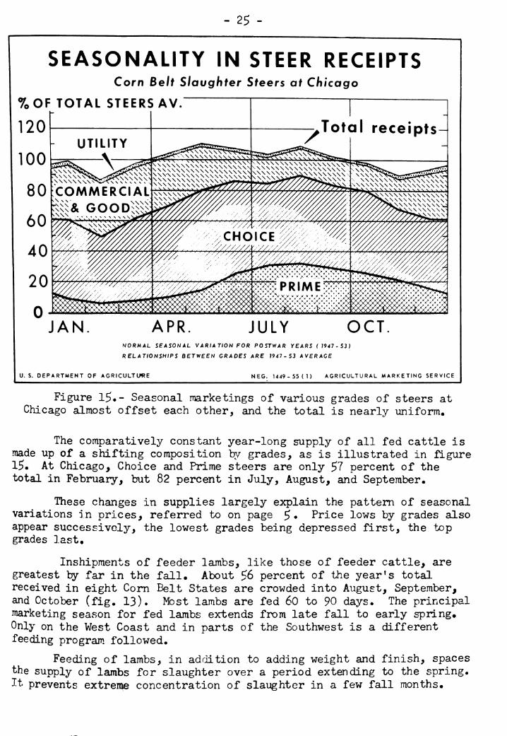
Figure 15«- Seasonal marketings of various grades of steers at Chicago almost offset each other, and the total is nearly uniform.

The comparatively constant year-long supply of all fed cattle is made up of a shifting composition by grades, as is illustrated in figure 15« At Chicago^ Choice and Prime steers are only 57 percent of the total in February, but 82 percent in July, August, and September*

These changes in supplies largely explain the pattern of seasonal variations in prices, referred to on page ^. Price lows by grades also appear successively, the lowest grades being depressed first, the top grades last.

Inshipments of feeder lambs, like those of feeder cattle, are greatest by far in the fall. About 56 percent of the year's total received in eight Com Belt States are crowded into August, September, and October (fig. 13). Most lambs are fed 60 to 90 days. The principal marketing season for fed lambs extends from late fall to early spring. Only on the West Coast and in parts of the Southwest is a different feeding program followed.

FeedJ-ng of lambs, in addition to adding weight and finish, spaces the supply of lambs for slaughter over a period extending to the spring. It prevents extreme concentration of slaughter in a few fall months*

- 26 -

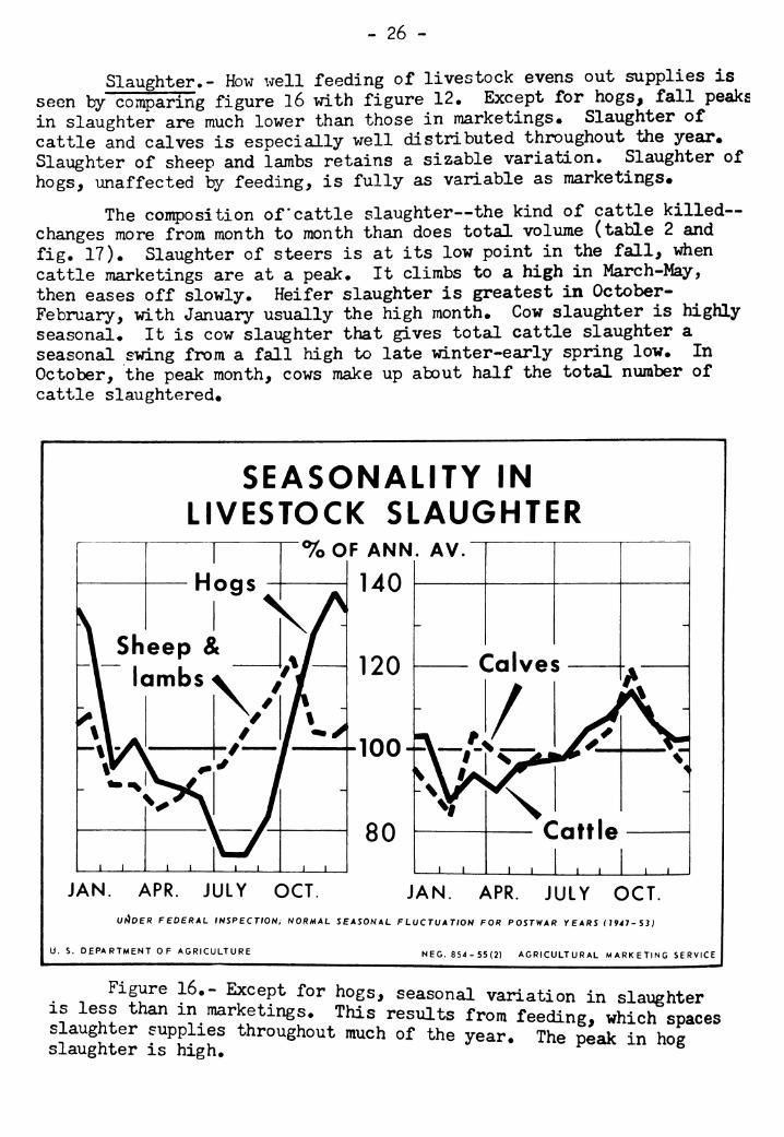
Slaughter.- How ^>rell feeding of livestock evens out supplies is seen by comparing figure l6 with figure 12, Except for hogs, fall peaks in slaughter are much lower than those in marketings. Slaughter of cattle and calves is especially well distributed throughout the year. Slaughter of sheep and lambs retains a sizable variation. Slaughter of hogs, unaffected by feeding, is fully as variable as marketings.

The composition of*cattle slaughter—the kind of cattle killed— changes more from month to month than does total volume (table 2 and fig. 17). Slaughter of steers is at its low point in the fall, when cattle marketings are at a peak. It climbs to a high in March-May, then eases off slowly. Heifer slaughter is greatest in October- February, with January usually the high month. Cow slaughter is highly seasonal. It is cow slaughter that gives total cattle slaughter a seasonal swing from a fall high to late winter-early spring low. In October, the peak month, cows make up about half the total number of cattle slaughtered.

SEASONALITY IN LIVESTOCK SLAUGHTER

%OF ANN. AV.

140 Hogs

J I I I I I I L

JAN. APR. JULY OCT. JAN. APR. JULY OCT. UI^DER FEDERAL INSPECTION; NORMAL SEASONAL FLUCTUATION FOR POSTWAR YEARS (1947-53

U. S. DEPARTMENT OF AGRICULTURE NEC. 854-55(2) AGRICULTURAL M ARK E TING SE R VICE

Figure 16.- Except for hogs, seasonal variation in slaughter IS less than in marketings. This results from feeding, which spaces slaughter supplies throughout much of the year. The peak in hog slaughter is high. ^ ^

- 27 -

SEASONALITY IN CATTLE SLAUGHTER BY CLASSES

% OF TOTAL CATTLE AV. " Total cattle

JAN APR JULY OCT. SLAUGHTER UNDER FEDERAL INSPECTION. NORMAL SEASONAL VARIATION FOR POSTWAR YEARS (1947-53).

RELATIONSHIPS BETWEEN CLASSES ARE 1944-53 AVERAGE.


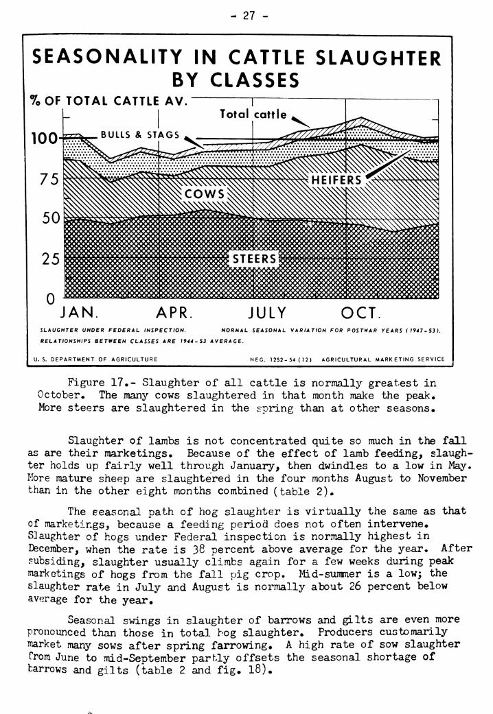
Figure 17•• Slaughter of all cattle is normally greatest in October* The many cows slaughtered in that month make the peak. More steers are slaughtered in the spring than at other seasons•

Slaughter of lambs is not concentrated quite so much in the fall as are their marketings. Because of the effect of lamb feeding, slaughter holds up fairly well through January, then dwindles to a low in May. More mature sheep are slaughtered in the four months August to November than in the other eight months combined (table 2).

The seasonal path of hog slaughter is virtually the same as that of marketings, because a feeding period does not often intervene. Slaughter of hogs under Federal inspection is normally highest in December, when the rate is 38 percent above average for the year. After subsiding, slaughter usually climbs again for a few weeks during peak marketings of hogs from the fall pig crop. Mid-summer is a low; the slaughter rate in July and August is normally about 26 percent below average for the year.

Seasonal swings in slaughter of barrows and gilts are even more pronounced than those in total hog slaughter. Producers customarily market many sows after spring farrowing. A high rate of sow slaughter from June to mid-September partly offsets the seasonal shortage of barrows and gilts (table 2 and fig. l8).

- 28 -

SEASONALITY IN HOG SLAUGHTER BY CLASSES*

%OF TOTAL HOGS AV.

120

JAN. APR. JULY OCT NORMAL SEASONAL VARIATION FOR POSTWAR YEARS (1947-53).

RELATIONSHIPS BETWEEN CLASSES ARE 1947-53 AVERAGE.

SUNDER FEDERAL INSPECTION. ÎNCLUDES A SMALL NUMBER OF STAGS AND BOARS.

U. S. DEPARTMENT OF AGRICULTURE NEC. 1262-54 (12) AGRICULTURAL MARKETING SERVICE

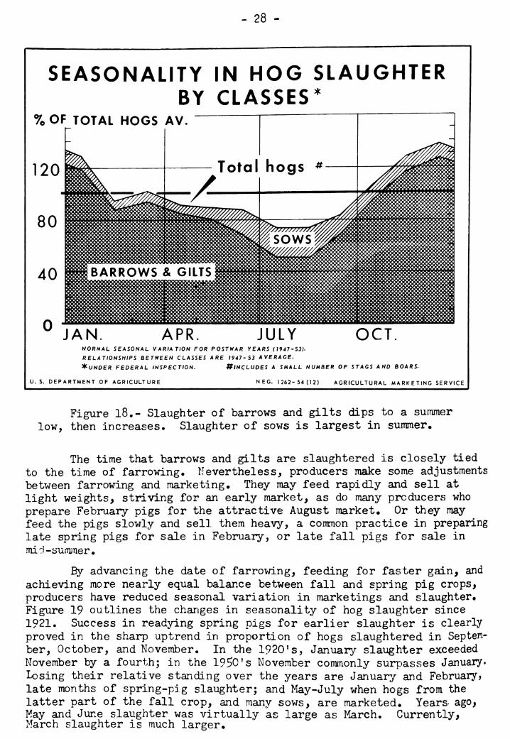
Figure 18*- Slaughter of barrows and gilts dips to a summer low, then increases. Slaughter of sows is largest in summer.

The time that barrows and gilts are slaughtered is closely tied to the time of farrowing. Nevertheless, producers make some adjustments between farrowing and marketing. They may feed rapidly and sell at light weights, striving for an early market, as do many producers who prepare February pigs for the attractive August market. Or they may feed the pigs slowly and sell them heavy, a common practice in preparing late spring pigs for sale in February, or late fall pigs for sale in mid-summer.

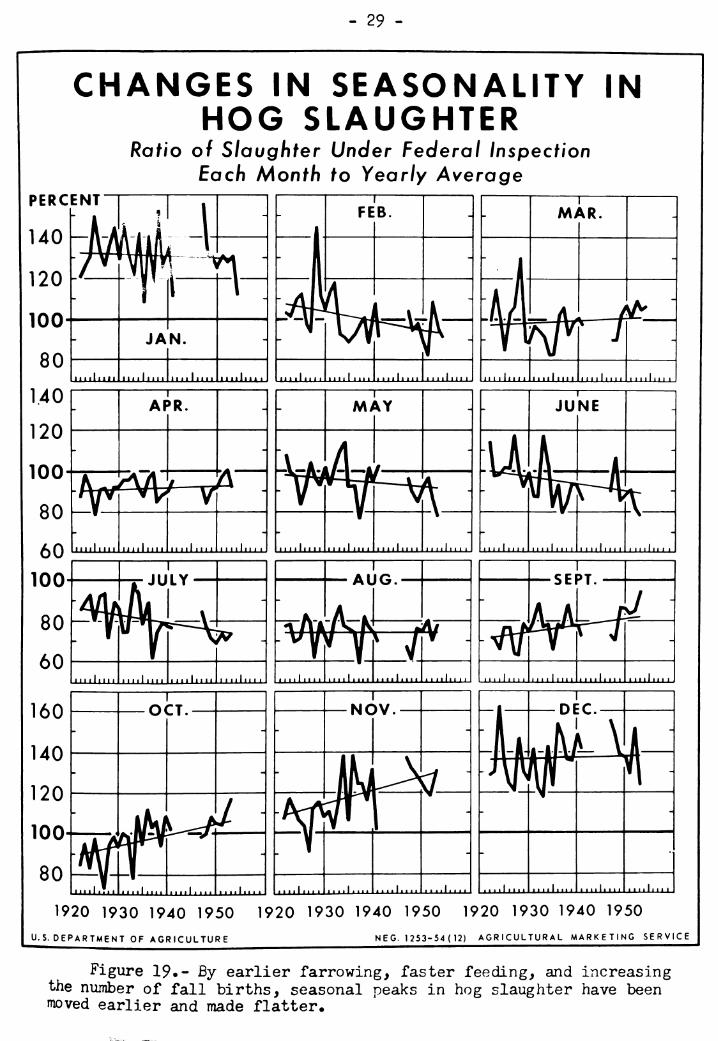
By advancing the date of farrowing, feeding for faster gain, and achieving more nearly equal balance between fall and spring pig crops, producers have reduced seasonal variation in marketings and slaughter. Fig\ire 19 outlines the changes in seasonality of hog slaughter since 1921. Success in readying spring pigs for earlier slaughter is clearly proved in the sharp uptrend in proportion of hogs slaughtered in Septem- ber, October, and November. In the 1920's, January slaughter exceeded November by a fourth; in the 1950's November commonly surpasses January, losing their relative standing over the years are January and February, late months of spring-pig slaughter; and May-July when hogs from the latter part of the fall crop, and many sows, are marketed. Years- ago> May and June slaughter was virtually as large as March. Currently, March slaughter is much larger.

- 29 -

CHANGES IN SEASONALITY IN HOG SLAUGHTER

Ratio of slaughter Under Federal Inspection Each Month to Yearly Average

PERCENT

1920 1930 1940 1950 1920 1930 1940 1950 1920 1930 1940 1950

U.S. DEPARTMENT OF AGRICULTURE NE G. 1253-54 ( 12) AGRICULTURAL MARKETING SERVICE

Figure 19«- By earlier farrowing, faster feeding, and increasing the niunber of fall births, seasonal peaks in hog slaughter have been moved earlier and made flatter.

- 30 -

Though the relative gain in size of- the fall pig crop lifted the position of March and April as slaughter months and reduced overall Variation in slaughter, its benefits are not unnaxed. As more sows are retained after spring farrowing for farrowing during ^^f^/^^.f ^ "^^^^ slaughtered during the summer is kept comparatively small. Ihis tends to make total hog slaughter in the summer even less than before.

PRODUCTION AND GONSUMPnON OF MEAT

Production of meat is larger or smaller month by month in about the proportion of the number of livestock slaughtered. Differences in live and dressed weight per head generally are not great. Barrows and gilts are heaviest in January and February, when producers niarket late spring-crop hogs they held past the December low in prices. Both cattle and sheep average heaviest in seasons that have the highest percentage of fed stock in total slaughter (table 3).

SEASONALITY IN COMMERCIAL MEAT PRODUCTION

7o OF ANN. AV

140

120

—/-^—100-

80- -i 1 1 1 \ 1 I I I I

JAN. APR. JULY OCT. JAN. APR. JULY OCT. NORMAL SEASONAL FLUCTUATION FOR POSTWAR YEARS ( 1947-53). EXCLUDES MEAT PRODUCED FROM FARM SLAUGHTER

U.S. DPPAf^TMENT nF AGRICULTURt NFo. I4I6-S.S(?' AC.ííirULTUR ^L V A k K e T IN G SR R VIC t

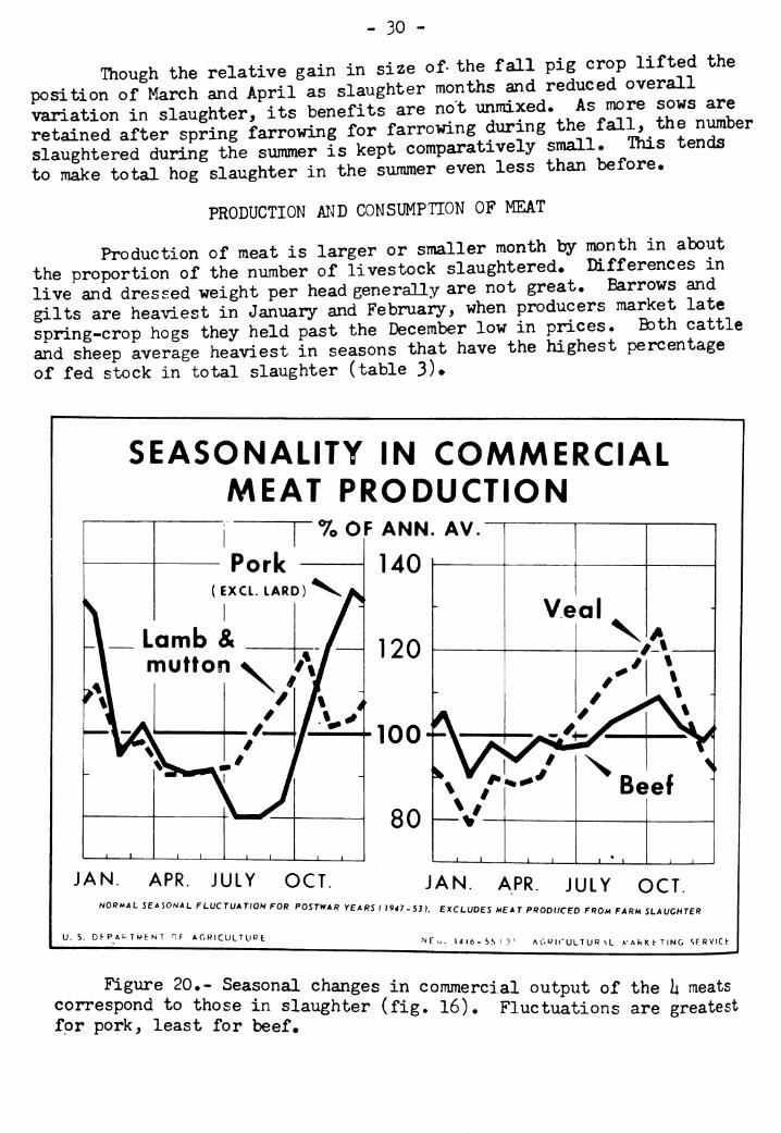
Figure 20♦- Seasonal changes in commercial output of the h meats correspond to those in slaughter (fig. 16)* Fluctuations are greatest for pork, least for beef.

- 31 -

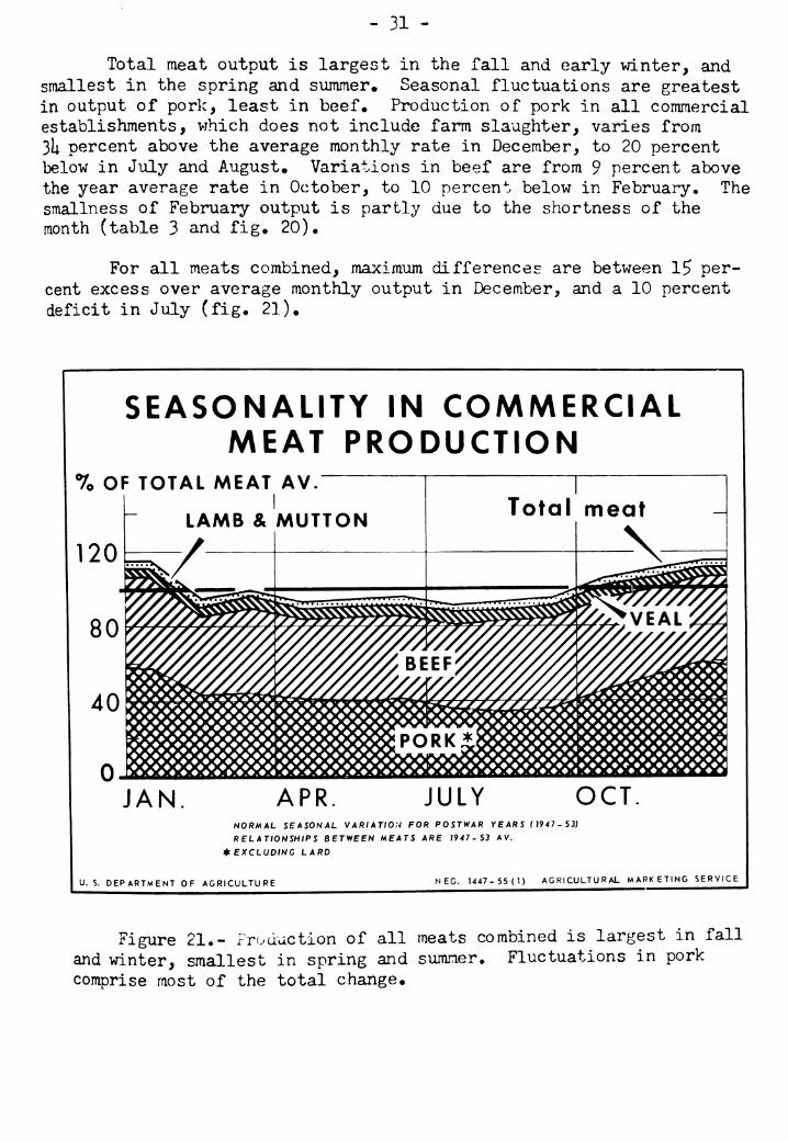
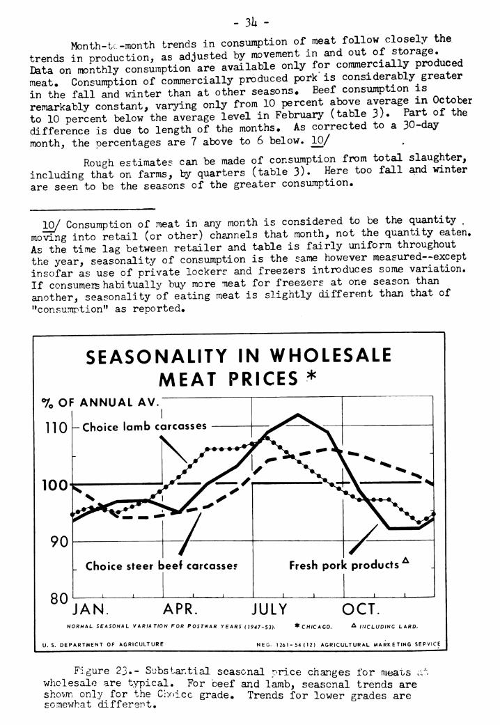
Total meat output is largest in the fall and early winter, and smallest in the spring and summer• Seasonal fluctuations are greatest in output of pork, least in beef» Production of pork in all commercial establishments, vihich does not include farm slaughter, varies from 3I; percent above the average monthly rate in December, to 20 percent below in July and August. Variations in beef are from 9 percent above the year average rate in October, to 10 percent below in February* The smallness of February output is partly due to the shortness of the month (table 3 and fig. 20).

For all meats combined, maximum differences are between 1^ percent excess over average monthly output in December, and a 10 percent deficit in July (fig. 21).

SEASONALITY IN COMMERCIAL MEAT PRODUCTION

7o OF TOTAL MEAT AV.

120

L

JAN APR. JULY OCT NORMAL SEASONAL VARIATION FOR POSTWAR YEARS (7947-53)

RELATIONSHIPS BETWEEN MEATS ARE 1947-53 AV.

ÊXCLUDING LARD


Figure 21.- Froduction of all meats combined is largest in fall and winter, smallest in spring and summer. Fluctuations in pork comprise most of the total change•

- 32 -

Table 3 •-Index numbers of normal month-to-raonth variation in Hveweight of meat animals marketed or slaughtered and in production, stocks and coneu>ç)tlon of meat 1/

\ : : : : : • ! r : : : :

Item : Jan. :

' Feb. • Mar. •Apr.

!

May June ! July s Aug.! ! Sept .:0ct.!Nov,:DBc.

five weif^ht per head :

Receipts at 8 markets Barrows and gilts : 10$ lOli 103 102 102 101 99 96 9li 95 98 101 Sows : 109 108 106 103 100 95 91 91 92 96 103 106

Slaughter under Federal inspection Cattle : 102 102 102 101 101 99 99 98 98 98 99 101 Calves : 95 87 82 8U 92 101 108 115 115 113 108 100 Sheep and lambs : 10Ü 106 107 101* 100 9i* 95 96 96 97 99 102 Hogs : 100 98 96 98 100 107 m 105 96 9U 96 99

Meat and lard produced per head of slaughter under Federal inspection Beef : 101.5 102.5 103.5 loU 102.5 100.5 100 98 97.5 95 96 99 Veal : 96 89 82 86 93 102 109 116 113 111 106 97 Lamb and mutton : lOli 106 107 105 101 95 95 96 96 96 98 101 Pork (excluding lard) : 99 98 97 98 99 105 109 106 98 96 97 98 Lard : lOli 102 98 98 103 108 112 102 90 89 9li 100

Tbtal production 2/ From Federally inspected slaughter

Beef : 105 89 98 9ti 99 97 98 103 105 109 102 101 Veal : 87 75 86 85 88 100 107 115 118 131 U2 96 Lamb and mutton : 112 98 99 90 90 90 91 100 107 118 101 lOli Pork (excluding lard) : 128 93 100 91 90 93 81 79 82 103 123 137

All meat ^ 115 91 98 92 9U 95 90 92 95 108 112 118

Lard ' 135 102 ; LOO 92 9U ^h. 85 76 73 93 116 lliO

From commercial slaughter 3/ Beef 105 90 98 9li 99 97 98 103 106 109 102 99 Veal ; 89 79 90 88 90 100 L06 nu 116 125 108 95 Lamb and mutton : 111 96 98 90 90 91 92 101 108 119 101 103 Pork : 128 9? ] L02 92 90 91 80 80 81*

97 103 la 13li

All meat : \\\x 92 99 93 9U 91* 90 93 108^ 111 115

Lard i 13U 103 101 93 91. 92 8U 77 75 9li 115 138 Cold storage stocks \x/

Beef : 13U 138 129 '120 106 91 76 70 7? 7ii 8l4 106 Veal : 156 139 IIU lOU 86 73 71 70 77 79 97 13li Lamb and mutton Pork j

All meat 5/ :

138 lía 130 112 86 79 76 71 71i 77 97 119 102 130 135 132 128 117 110 96 71i 55 50 71 110 130 130 127 120 110 102 92 7U 63 62 80

Consumption \ Commercially produced meat 2/ 6/ :

Beef " * Veal : Lamb and mutton Pork .

All meat .

105 90 98 9U 99 97 98 103 107 110 101 98 92

111 81 96

92 99

89 91

90 90

99 105 113 91 92 101

115 108

12a 105 95 119 100 102

127 9Í» 102 92 90

9U 91 81 81 85 103 la 133

llU 92 99 93 91» 91 9U 98 108 110 113

From total slaughter Beef Veal \ 98

90 02

97 101 10Ü Lamb and mutton 1

92 109 109 Pork

X 90 100 108 luy 90 80 121 All meat . 103 93 92 112

:

1/ Percentage ratio of each month to the year average as 100. 1/ Not corrected for differences in length of month» 3/ Includes federally inspected and all other commercial slaughter. y First of month.

Normal values for postwar years (19U7-53).

Excludes farm slaughter.

- 33 -

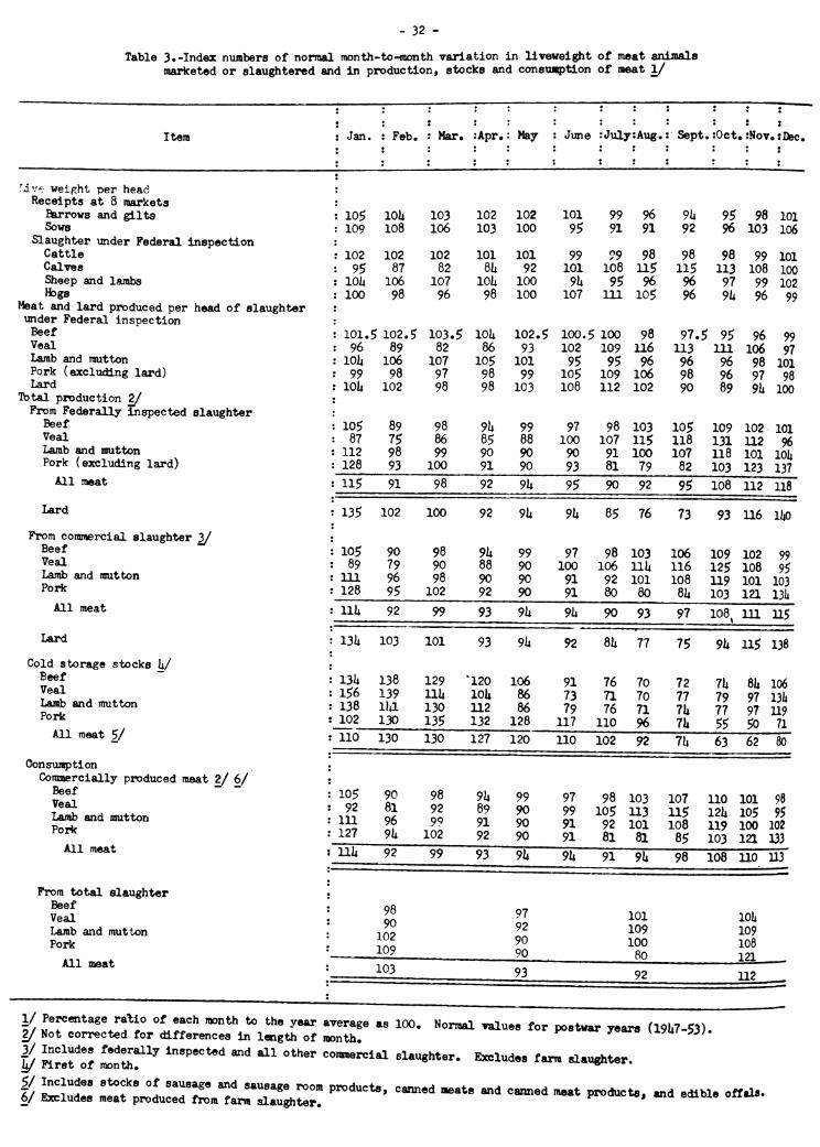
Meat is placed in cold storage in winter for sale in suiraner. Storage of pork amounts to about three-fourths of all meat stored, not counting miscellaneous meat products. The peak stock, about March 1, usually equals about 6 percent of a year's total pork supply. Low point for pork stocks is normally around November 1 (table 3 and fig. 22).

Most beef put in storage is cow beef, held to be sold as sausafê and other processed products during summer. Beef stocks ordinarily are at peak vcûme February 1. Their quantity at this time is approximately 2 percent of a year's production. For veal, January 1, and for lamb, February 1, mark the biggest storage holdings.

SEASONALITY IN STOCKS OF MEAT IN COLD STORAGE

7o OF TOTAL MEAT AV.

120

Total meat

OTHER MEAT*

JAN APR JULY OCT NORMAL :>£ASONAL VARIATION FOR POSTWAR YE ARS, 1947 - 53

RELATIONSHIPS BETWEEN MEATS ARE 1947-53 AVERAGE

* INCLUDES SAUSAGE AND SAUSAGE ROOM PRODUCTS. CANNED MEATS

AND CANNED MEAT PRODUCTS, AND EDIBLE OFFALS

U. S. DEPARTMENT OF AGRICULTURE NEC. 1448-55(1) AGRICULTURAL MARKCTING SERVICE

Figure 22•- Sale of meat out of cold storage holdings, built to a high in the winter, adds to the supply available for spring and summer consumption*

- 3U -

Month-tc-month trends in consumption of meat follow closely the trends in production, as adjusted by movement in and out of sto^^S^. Data on monthly consumption are available only for commercxally produced meat. Consumption of commercially produced pork is considerably greater in the fall and winter than at other seasons. Beef consumption is remarkably constant, varying only from 10 percent above average in October to 10 percent below the average level in February (table 3). Part of the difference is due to length of the months. As corrected to a 30-day month, the percentages are 7 above to 6 below. 10/

Rough estimates can be made of consumption from total slaughter, including that on farms, by quarters (table 3). Here too fall and winter are seen to be the seasons of the greater consumption.

10/ Consumption of meat in any month is considered to be the quantity . mo^ng into retail (or other) ch?jinels that month, not the quantity eaten. As the time lag between retailer and table is fairly uniform throughout the year, seasonality of consumption is the same however measured—except insofar as use of private lockers and freezers introduces some variation. If consumers habitually buy more meat for freezers at one season than another, seasonality of eating meat is slightly different than that of "consumption" as reported.

SEASONALITY IN WHOLESALE MEAT PRICES *

% OF ANNUAL AV.

110

100

I -Choice lamb carcasses

80

_ Choice steer beef corcassef Fresh pork products

JAN APR JULY OCT. NORMAL SEASONAL VARIATION FOR POSTWAR YEARS (1947-53). ^CHICAGO. ^ INCLUDING LARD.

U.S. DEPARTMENT OF AGRICULTURE NEG. 1261-54(12) AGRICULTURAL MARKETING SERVICE

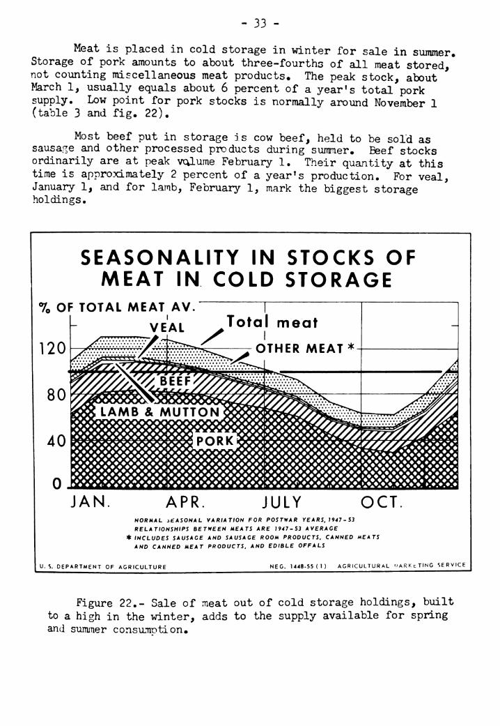
Figure 23.- Substantial seasonal price changes for meats at wholesale are typical. For beef and lamb, seasonal trends are shovm only for the Ciioice grade« Trends for lower grades are scmev/hat different.

- 35 -

PRICES OF MEAT

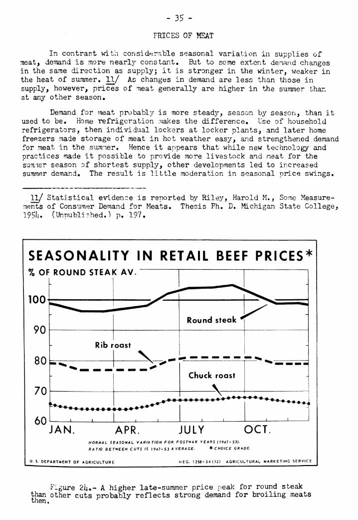
In contrast with considerable seasonal variation in supplies of meat, demand is more nearly constant. But to some extent denarid changes in the same direction as supply; it is stronger in the winter, weaker in the heat of summer* 11/ As changes in demand are less than those in supply, however, prices of meat generally are higher in the summer than at any other season«

Demand for meat probably is more steady, season by season, than it used to he. Home refrigeration nialces the difference« Use of household refrigerators, then individual lockers at locker plants, and later home freezers made storage of meat in hot weather easy, and strengthened demand for meat in the summier. Hence it appears that while new technology and practices made it possible to provide more livestock and neat for the sunfiier season of shortest supply, other developments led to increased summer demamd. The result is little moderation in seasonal price swings»

11/ Statistical évidence is reported by Riley, Harold M., Some Measure- ments of Consumer Demand for Meats« Thesis Ph« B. Michigan State College, 195Î4* (Unpublished.) P* 197.

SEASONALITY IN RETAIL BEEF PRICES* % OF ROUND STEAK AV

100

JAN APR. JULY OCT. NORMAL SEASONAL VARIATION FOR POSTWAR YEARS (1947-53).

RATIO BETWEEN CUTS IS 1947-5 3 A VER AGE. t CHOICE GRADE


Figure 2Í4,- A higher late-summer price peak for round steak than other cuts probably reflects strong demand for broiling meats tlien •

- 36 -

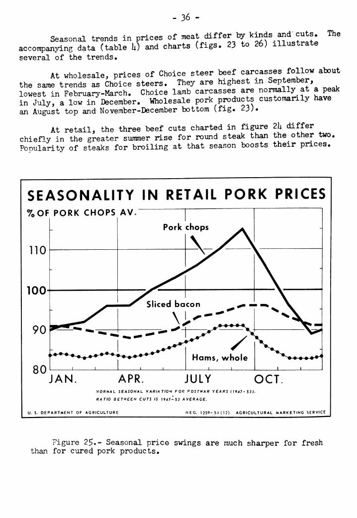
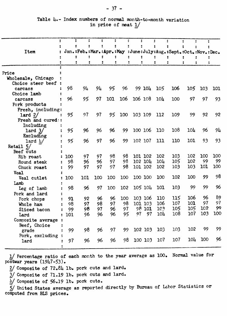
Seasonal trends in prices of meat differ t^ kinds and cuts. The accompanying data (table k) and charts (figs. 23 to 26) illustrate several of the trends.

At wholesale, prices of Choice steer beef carcasses follow about the same trends as Choice steers. They are highest m September, lowest in February-March. Choice lamb carcasses are normally^ at a peak in July, a low in December. Viholesale pork products customarily have an August top and November-December bottom (fig. 23).

At retail, the three beef cuts charted in figure 2U differ chiefly in the greater summer rise for round steak than the other two. Ponularity of steaks for broiling at that season boosts their pnces.

SEASONALITY IN RETAIL PORK PRICES %OF PORK CHOPS

1

AV.

- Pork chops y^ -

no \X N -

^

V/^

\

IÜÜ- ^ \

^^^

—/^ Sliced ba con ^ -

90 ^ •• •% ^ ^^^^^^„-^

Hams, whole 1 1

V on II II 1 1

JAN APR. JULY OCT .V0RA4AL SEklOUkL VARIATION FOR POSTWAR Y EARS (1947 - 53)-

RATIO BETWEEN CUTS IS 1947-53 AVERAGE.


Figure 25.- Seasonal price swings are much sharper for fresh than for cured pork produets«

- 37 -

Table U«- Index numbers of normal month-to-raonth variation in price of meat 1/

Item : Jan« j íFeb» ! ¡Mar.! ÍApr«1 ¡May ! ¡June; ¡July; ¡Aug.i iSept,; ¡Oct. « ¡Nov. ; ¡Dec.

Price : Wholesale, Chicago :

Choice steer beef ; carcass : 98 9U 9U 95 96 99 lOU 105 106 105 103 101

Choice lamb : carcass : 96 95 97 101 106 106 108 lOU 100 97 97 93 Pork products : Fresh, including; lard 2/ \ 95 97 97 95 100 103 109 112 109 99 92 92 Fresh and cured;!

Including lard 3/ \ 95 96 96 96 99 100 106 110 108 lOli 96 ^\x Excluding lard \x/ \ 95 96 97 96 99 102 107 111 110 101 93 93

Retail 5/ Beef cuts Rib roast : 100 97 97 98 98 101 102 102 103 102 100 100 Rovind steak : 98 96 96 97 98 102 lOU lOU 105 102 99 99 Chuck roast : 99 97 97 97 98 101 102 102 103 103 101 100

Veal Veal cutlet : 100 101 100 100 100 100 100 100 102 100 99 98

Lamb Leg of lamb i 98 96 97 100 102 105 lOii 101 103 99 99 96

Pork and lard Pork chops *: 91 92 96 96 100 103 106 110 115 106 96 89 Whole ham : 98 97 98 97 98 101 103 106 107 101 97 97 Sliced bacon : 99 98 97 96 97 98 101 103 105 105 102 99 Lard : 101 96 96 96 95 97 97 loU 108 107 103 100

Composite average Beef, Choice grade \ 99 98 96 97 99 102 103 103 103 102 99 99

Pork, excluding lard \ 97 96 96 96 98 100 103 107 107 lOli 100 96

1/ Percentage ratio of each month to the year average as 100, Normal value for postwar years (19U7-53).

2/ Composite of 72.eU lb. pork cuts and lard. 3/ Composite of 71.19 lb. pork cuts and lard. y Composite of 56.19 lb. pork cuts. y United States average as reported directly by Bureau of Labor Statistics or

coinputed from BLS prices.

- 38 -

SEASONALITY IN RETAIL PRICES 7o OF ANNUAL AV.

90 no

100

90

VEAL CUTLETS

J L J L

JAN. APR

-1 L _J L_

LEG OF 1 .AMB

1 1 1 1 1 1 1 1

JULY OCT. NORMAL SEASONAL VARIATION FOR POST'ÂR Y E ARS ( 1 947 - 53 )■


Figure 26.- Prices of veal cutlets are stable month to months Leg of lamb traces about the same price pattern as Choice lamb carcasses»

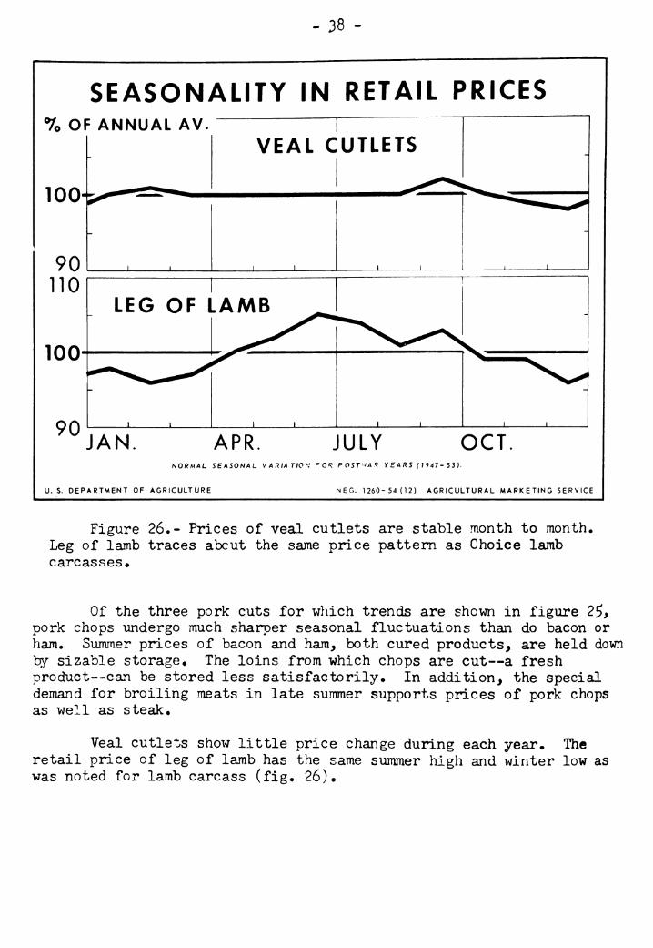
Of the three pork cuts for wliich trends are shown in figure 25> pork chops undergo much sharper seasonal fluctuations than do bacon or ham. Summer prices of bacon and ham, both cured products, are held down by sizable storage♦ The loins from which chops are cut—a fresh product—can be stored less satisfactorily. In addition, the special demand for broiling meats in late summer supports prices of pork chops as well as steak.

Veal cutlets show little price change during each year. The retail price of leg of lamb has the same summer high and winter low as was noted for lamb carcass (fig. 26)•

- 39 -

RELIABILITY OF SEASONAL INDEXES

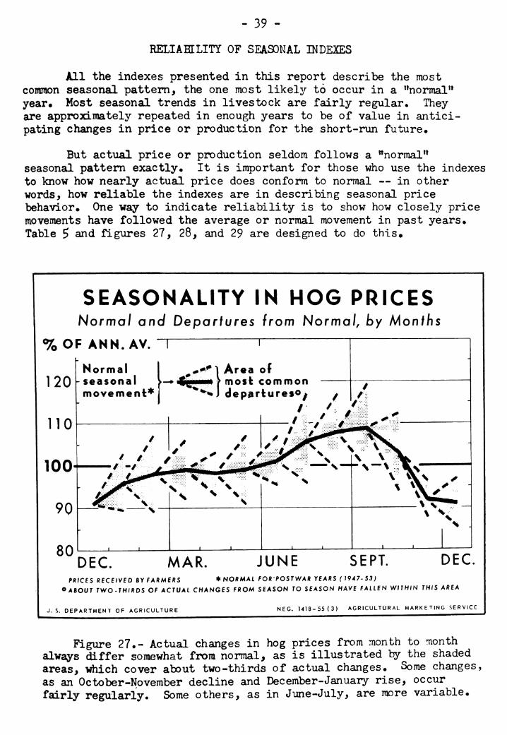
All the indexes presented in this report describe the most comraon seasonal pattern, the one most likely to occur in a "normal" year» Most seasonal trends in livestock are fairly regular♦ They are approximately repeated in enough years to be of value in antici- pating changes in price or production for the short-run future»

But actual price or production seldom follows a "normal" seasonal pattern exactly» It is important for those who use the indexes to know how nearly actual price does conforra to normal — in other words, how reliable the indexes are in describing seasonal price behavior» One way to indicate reliability is to show how closely price movements have followed the average or normal movement in past years» Table 5 and figures 27, 28, and 29 are designed to do this»

SEASONALITY IN HOG PRICES Norma/ and Deparfures from Normal, by Monfhs

% OF ANN. AV. "1 I

120

110

100

90

80

Normal seasonal movement^

^^^^\ Area of i-^fîfg^mm fm OS fc common

*^j dep^rfcureso^ ^

DEC. MAR. JUNE SEPT. DEC. PRICES RECEIVED BY FARMERS ♦NORMAL FORPOSTV/AR YEARS (1947-53)

O ABOUT TWO-THÍRDS Of ACTUAL CHANGES FROM SEASON TO SEASON HAVE FALLEN WITHIN THIS AREA

J. S. DEPARTMENT OF AGRICULTURE NEC. 1418-55(3) AGRICULTURAL MARKETING SERVICE

Figure 27•- Actual changes in hog prices from month to month always differ somewhat from normal, as is illustrated by the shaded areas, which cover about two-thirds of actual changes. Some changes, as an October-November decline and Dec ember-January rise, occur fairly regularly. Some others, as in June-July, are more variable*

- liO -

Figure 27 shows the extent to which month-to-month changes in

prices reSived for hogs have departed from the normal ^^^"f^-. ^^^^^f^J is drawn so that the most common price changes from one "^f^ to the next- those occurring in approximately two-thirds of the 28 êars stuêd-all fall within the limits of the shaded areas. From December to January, the »»normal« postwar experience is a price rise of 5 percent ^Hl^l annual average)-fn>m 91 percent to 96 percent. In any g^^^"/Jf P^^^^ will probably go up more or less than ^ percent. The probability is that in 2 years oÍt of 3, actual changes will fall within an ^^^J^^f °f^ , ^^ 12 percent and a decrease of 2 percent. Prices thus go up from D^jember to January in most years, but the size of the increase vanes considerably.

Prices of hogs usually rise in Dec ember-January and increase with much regularity in May-June and June-July. In 26 out of 28 years they have declined in October-November. Declines are typical also m September- October and November-December. Trends between other pairs of months have

been more variable. .

SEÁSONALITY IN HOG PRICES Normal and Departures from Norma/, by Seasons

% OF ANN. AV. T

Normal -i***1 Area of 120 -seasonal >— Í; > most common ~^

movement* "^^J departures^ •

no

100

90

80 DEC. MAR. JUNE SEPT. DEC.

PRICES RECEIVED BY FARMERS «NORMAL FOR POSTWAR YEARS (1947-53)

OABOUT TWO-THIRDS OF ACTUAL CHANGES FROM SEASON TO SEASON HAVE FALLEN WITHIN THIS AREA


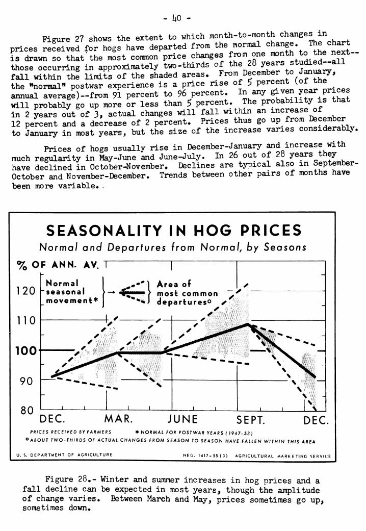
Figure 28•- Winter and siimmer increases in hog prices and a fall decline can be expected in most years, though the amplitude of change varies• Between March and May, prices sometimes go up, sometimes down»

. ai.

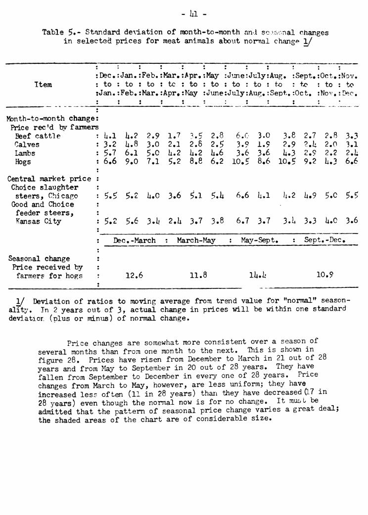
Table $•• Standard de\lation of month-to-month and sc.^ônal changes in selected prices for meat animals abo\it nonial change 1/

Item Dec* : Jan. :Feb. :Kar* :Apr# :May :J\:aie: July: Aug. :Sept* :Oct* :Nov. to : to : to : to : to : to : to : to : to : fx> : to : to

Jan.:Feb.:Mar.:Apr»:KÄy :June:July:Aug.:Sept. :Oct. :Nov.:Dec.

îfenth-to-month change Price rec'd by farmers

Beef cattle i U.l ii.? 2.9 1.7 ?.5 2.8 6.0 3.0 3.8 2.7 2.8 3.3 Calves ! 3.2 U.8 3.0 2.1 2.6 2.5 3.9 1.9 2.9 2.h 2.0 3.1 Lambs ! 5.7 6.1 5.0 U.2 U.2 U.6 3.6 3.6 U.3 2.9 2.2 2.1; Hogs 1 ; 6.6 9.0 7.1 5.2 8.8 6.2 10.5 8.6 10.5 9.2 h.3 6.6

Central market price : Choice slaTJghter ! steers, Chicago : 5.5 5.2 U.C 3.6 5.1 5.U 6.6 U.l h.2 U.9 5.0 ^.^.

Good and Choice ! feeder steers. Kansas City- : 5.2 5.6 3.1' 2.U 3.7 3.8 6.7 3.7 3.1 3.3 U.C 3.6

: Dec,-March : March-May : May-Sept« • Sept .-Dec •

Seasonal change Price received by

farmers for hogs 12.6 11.8 lk*h 10.9

1/ Deviation of ratios to moving average from trend value for "normal'* season- alTty. In 2 years out of 3, actual change in prices will be within one standard deviatior. (plus or minus) of normal change.

Prtce changes are somewhat more consistent over a season of several months than from one month to the next. This is shown in figure 28. Prices have risen from December to March in 21 out of 28 years and from May to September in 20 out of 28 years. They have fallen from September to December in every one of 28 years. Price changes from March to May, however, are less uniform; they have increased less often (11 in 28 years) than they have decreased 0-7 in 28 years) even though the normal now is for no change. It mu£>i be admitted that the pattern of seasonal price change varies a great deal; the shaded areas of the chart are of considerable size.

- 12 -

SEASONALITY IN CATTLE PRICES Normal and Departures from Normal, by Months

% OF ANN. AV.n \

120

no

100

90

80

Normal |- seasonal

movement

^^/^ I Area of —► wfmmm > most common

^^% j departures^

DEC. MAR. JUNE SEPT. DEC. PRICES OF BEEF CATTtE RECE/VED BY FARM ERS ♦ NORMAl FOR POSTWAR YEARS (}947-S1 )

"ABOUT TWO-THIRDS OF ACTUAL CHANGES FROM SEASON TO SEASON HAVE FALLEN WITHIN THIS AREA

U.S. DEPARTMENT OF AGRICULTURE MEG. U15-SS(3) AGRICULTURAL MARKETING SERVICE

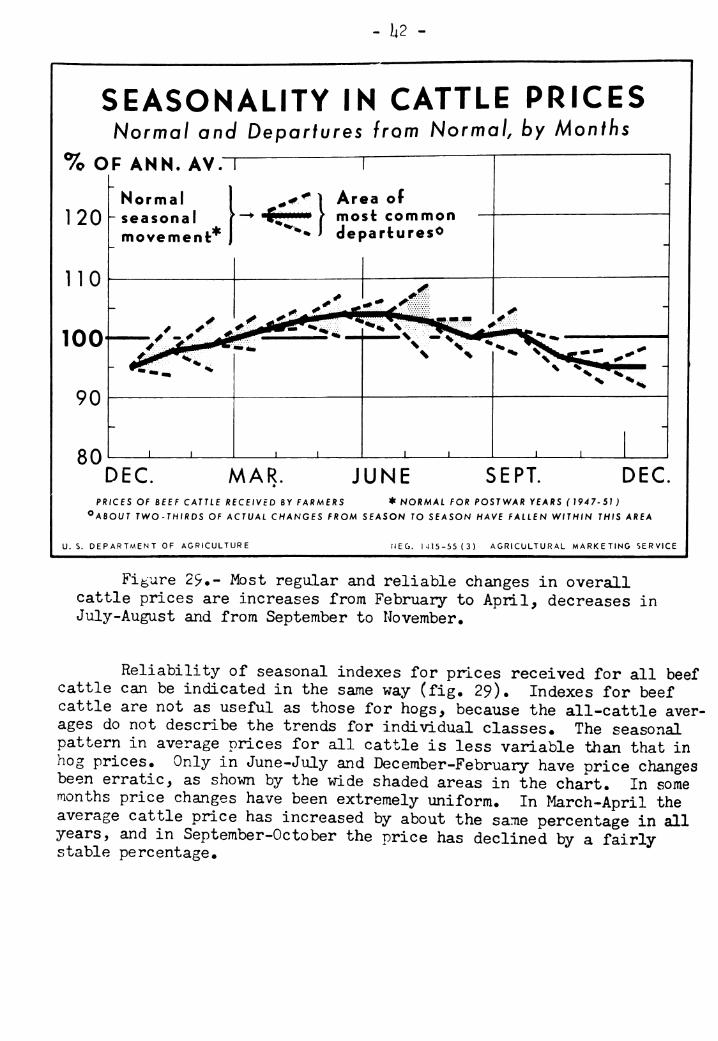
Figure 29»- Most regular and reliable changes in overall cattle prices are increases from February to April, decreases in July-August and from September to November,

Reliability of seasonal indexes for prices received for all beef cattle can be indicated in the same way (fig. 29). Indexes for beef cattle are not as useful as those for hogs, because the all-cattle aver- ages do not describe the trends for individual classes. The seasonal pattern in average prices for all cattle is less variable than that in hog prices. Only in June-July and December-February have price changes been erratic, as shown by the wide shaded areas in the chart. In some months price changes have been extremely uniform. In March-April the average cattle price has increased by about the same percentage in all years, and in September-October the price has declined by a fairly stable percentage.

Price trends are less consistent for Choice slaughter steers. The standard deviations in table 5 for prices of this grade at Chicago are rather large in most months, though much smaller than those for hog prices* Prices of Choice slaughter steers are especially inconsistent at rriid-x^nter and mid-summer» This means that the vanter decline, while almost always occurring, sometimes is earlier than usual and sometimes later* The price recovery due in early summer sometimes appears on schedule, and sometimes does not. But the July-September price rise is much more dependable*

Standard deviation data for prices of Good and Choice feeder steers at Kansas City indicate clearly the times of year when price trends are comparatively consistent, and therefore predictable, and when they are less so. For March-April the figure is only 2.U, and for adjoining months, 3«U and 3«7; thus an advance in feeder prices from' February to May can be counted on rather safely in most years. But June-July is a hazardous, unpredictable time. The value of 6.7 shows how untrustworthy ''normal*^ price trends are at that time. Depending on progress of new grazing and the completeness of restocking, prices in June sometimes rise to a season high, in other years dip sharply during the month. In 1953, prices touched their year's low in late June# Price trends for feeder steers in late summer and early fall are much more dependable. Their direction is almost always downward, though the amount of decrease varies from year to year.

Lacking other information, the producer or marketing man can refer to the normal seasonal pattern as the best single guide to future trends in production, marketings, or prices. The data and charts presented here are good starting points. But he can do even more. He can take account of other information to tell whether a trend is likely to differ from normal. If trends in business conditions and consumer demand for meat are sharply upward, price trends for livestock and meat will ordinarily be tilted up from normal* If demand is declining, prices vdll tend to sag. If livestock production has been increasing, the fall seasonal increase in marketings and decrease in prices are likely to be greater than normal. In 195U, for example, an increase in hog production brought a prolonged downtrend in hog prices. Because of it, the usual seasonal rise at mid-summer was almost eliminated and the total decline to December was much greater than normal.

Market and outlook reports will help portray the seasonal trends in prospect at any time. Market news reports provide a running record of marketings and trices throughout the United States. Reports on the pig crops and the lamb crop and quarterly reports of cattle on feed provide vital information that indicate prospective marketings. Outlook statements such as the Livestock and Meat Situation describe trends and developments in detail, both current and anticipated. 12/

12/ All reports available from Agricultural Marketing Service, U. S. Dept, Agr., Wash., D. C. The Extension Service of most States also publishes weekly or monthly outlook reviews*

- uu - All such current information can be used to modiiy the indexes

of normal seaconality, so that one's expectations of trends a month or a season ahead can be adjusted to the specific conditions of that season.

APPLICATION: HDW SEASOllAL INDEXES CAN BE USED

Granting that a normal seasonal index is an acceptable indicator of probable seasonal trends, and that it is even better when modified according to conditions in a given year, the next question is how it can be used. In what way can seasonal data be applied to actual pro- blems in management?

The flexibility—the wide choice of decisions—open to livestock producers affords broad scope to use of economic information. More than h million farmers and ranchers produce livestock, most of them in relatively small units, each independently of the other. Every producer must repeatedly make decisions in producing and marketing his livestock, and he has many options available to him.

A producer who aims for high-price seasons for marketing must be attentive to seasonal trends. Recognizing seasonality in prices of fed steers, some feeders have adopted a delayed feeding program that allows them to sell in the fall when prices for well finished fed cattle are frequently at their highest. Some producers who customarily had sold calves and yearlings at the end of the grazing season have since learned to accumulate enough winter roughage to hold at least part of their stock for winter or early spring sale. Often slaughter cows have been sold in October as much by habit as by necessity. Frequently, that low-price month can easily be avoided.

As livestock approach market weight, knowledge of normal seasonal trends and of the current situation is of aid in choosing the week in v/hich to sell. 13/

An alert producer can often take advantage of unusual price trends of short duration that occasionally appear—and earn much profit thereby» Buyers of feeder steers, habituated to late-summer or fall purchase, vjere slow to respond to the severely depressed prices in June 1953j whan a heat wave and drought threw unusually large supplies of grass cattle on the market. The few who did buy at that time realized exceptionally large, profits. But it is admittedly hard to know when low prices are genuine bargains. The falling prices for feeders in 1952 did not result in high feeding profits because that decline was part of a broad and lasting cyclical movement.

13/ Indexes of seasonal trendr by weeks may be of more value than the monthly indexes presented here. Weekly price movements for slaughter steers are reported in Hunter, Donald J., and Kutish, Francis A*, Weekly Beef Cattle Seasonal Price Patterns. Iowa Fain Science. September 19Sh^

- U5 -

Producers of lambs have a choice between planning for the early summer market or the late market« Considerably higher prices have often been received for the early marketings• But as marketings have been increased at the early period a price benefit has been realized less regularly« As was noted on page 12, the price advantage in June over later months has been diminishing of late. Nevertheless, there is still enough chance of higher prices early in the summer to make early marketing attractive to lamb producers who can achieve it readily.

Seasonal variations in prices of slaughter hogs are wider than those of other meat animals. Information on seasonality has as much or more application to hogs than to any other species of livestock« It can be used effectively to help producers plan their production and marketing programs.

As was seen in figures 7 and !^, seasonal changes in prices of hogs differ slightly by weight groups. Price increases and decreases generally connence later for the heavier weights.

Obviously, a producer will profit if, without too much extra cost, he can have his hogs ready for marketing in a high price period. Tied in with a choice as to when to sell is the weight at which to sell. At some seasons it pays to sell early and light. At other times the return is greater by holding hogs longer for sale at heavier weight,

A hog held an extra week or two moves into a heavier weight classification. Thus, the price for a 190 pound hog, on, say, September 1 would be compared with the normal value September 15 for a 220 pound hog. Calculations of this kind can readily be made, lU/ The index for a 190 pound hog September 1 is about 110 (midway between 113 for August and 107 for September) • For a 220 pound hog on September 15 it is about 109*5# The normal price decline thus is small. If the September 1 price is $20,00, that of September .15 is computed as $19»90, The 190 pound hog is worth $38.00, the 220 pound hog $U3.80, The extra 30 pounds return $5*80, or s$19#35 per 100 pounds. Each producer can calculate whether the cost of gain is this high. Usually it is not. At $1*50 com, average cost for extra gain is around $16.50, In an average or normal year, holding light-v;eight hogs past September 1 is profitable. Similar computations for other periods will demonstrate how well a producer profits by holding hogs to heavier weights in a season of rising prices, and how much he gains by selling light ahead of a price downtrend.

11/ A method, with illustrative data, is outlined more fully in Seasonal Variation in Prices of Barrows and Gilts, The Livestock and Meat wîtuation. Hay 7, 195U, p# 17, Separates are available on request to Information Division, Agricultural Iferketing Service, U. S. Dept. of Agr,

. US -

Costs of Altering Programs>- To most producers some disadvantage and cost is involved in adjusting production and marketing to capitalize on seasonally high prices* There is a feed cost in holding grass cattle past the fall marketing season. Costs of gain in feeding cattle are usually higher for the higher finish* To farrow pigs early for summer marketings, there is extra expense for better housing and artificial heat* In calculating the return from putting added weight on a market hog^ the cost of that gain must be known* Each producer who tries to adjust to seasonal trends must decide whether potential return is equal to the cost^

Application to the Meat Trade and Consumers*- The meat packing industry seeks constantly to regulate its policies in accumulating or dispensing meat from cold storage according to the seasonal price trends in prospect* The industry is necessarily alert to both normal and abnormal seasonal price behavior• Consumers of meat, both private and institutional, who have cold storage freezers or lockers can often consider seasonal price movements in deciding when to refill their spaces* And in many less explicit ways, consumers' knowledge of seasonal trends in meat animals and meats can serve a highly useful purpose*

TÍr U. S. GOVERNMENT PRINTING OFFICE: 1955 O—345151