Embed Size (px)
Citation preview

1
Module 4b: Water Distribution System
Design
Hardy Cross M
ethod
Robert Pitt
University of Alabam
a
and
Shirley Clark
Penn State -Harrisburg
Hardy Cross M
ethod
•Used in design and analysis of water
distribution systems for many years..
•Based on the hydraulic form
ulas we reviewed
earlier in the term
.
For Hardy-Cross Analysis:
•Water is actually rem
oved from the distribution system
of a
city at a very large number of points.
•Its is not reasonable to attem
pt to analyze a system with this
degree of detail
•Rather, individual flows are concentrated at a sm
aller number
of points, commonly at the intersection of streets.
•The distribution system can then be considered to consist of a
network of nodes (corresponding to points of concentrated
flow withdrawal) and links (pipes connecting the nodes).
•The estimated water consumption of the areas contained
within the links is distributed to the appropriate nodes
Netw
ork
mo
del o
verl
aid
on
aeri
al p
ho
tog
rap
h
(Walski, et al.2004 figure 3.4)
2
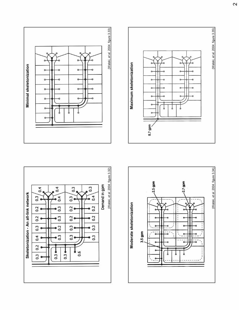
Skele
ton
izati
on
-A
n a
ll-l
ink n
etw
ork
(Walski, et al.2004 figure 3.32)
Min
imal skele
ton
izati
on
(Walski, et al.2004 figure 3.33)
Mo
dera
te s
kele
ton
izati
on
(Walski, et al.2004 figure 3.34)
Maxim
um
skele
ton
izati
on
(Walski, et al.2004 figure 3.35)

3
(Walski, et al.2001 figure 7.17)
Cu
sto
mers
mu
st
be s
erv
ed
fro
m s
ep
ara
te p
ressu
re z
on
es
Pro
file
of
pre
ssu
re z
on
es
(Walski, et al.2001 figure 7.20)
Pre
ssu
re z
on
e t
op
og
rap
hic
map
(Walski, et al.2001 figure 7.21)
Imp
ort
an
t ta
nk
ele
vati
on
s
(Walski, et al.2001 figure 3.10)
4
Sch
em
ati
c n
etw
ork
illu
str
ati
ng
th
e u
se o
f a p
ressu
re
red
ucin
g v
alv
e
(Walski, et al.2001 figure 3.29)
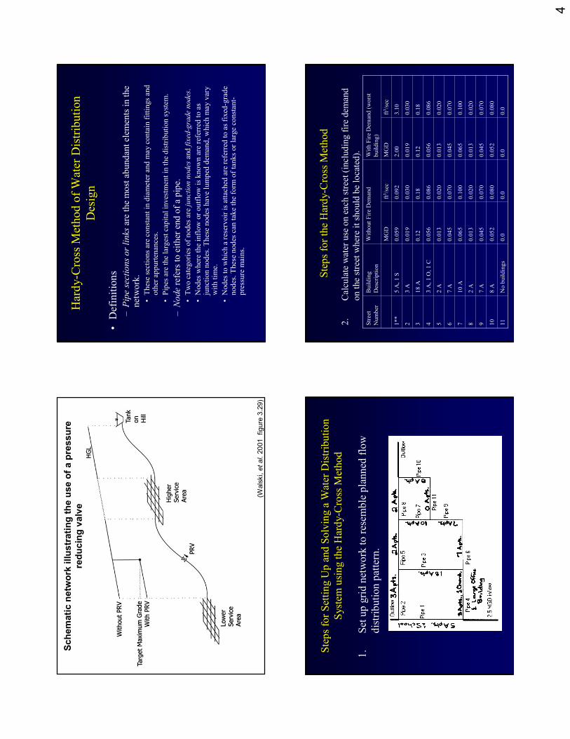
Hardy-C
ross M
ethod of Water Distribution
Design
•Definitions
–Pipe sections or links
are the most abundant elem
ents in the
network.
•These sections are constant in diameter and m
ay contain fittingsand
other appurtenances.
•Pipes are the largest capital investm
ent in the distribution system
.
–Noderefers to either end of a pipe.
•Two categories of nodes are junction nodes
and fixed-grade nodes.
•Nodes where the inflow or outflow is known are referred to as
junction nodes. These nodes have lumped dem
and, which m
ay vary
with tim
e.
•Nodes to which a reservoir is attached are referred to as fixed-grade
nodes. These nodes can take the form
of tanks or large constant-
pressure m
ains.
Steps for Setting Up and Solving a W
ater Distribution
System
using the Hardy-Cross M
ethod
1.
Set up grid network to resem
ble planned flow
distribution pattern.
Steps for the Hardy-Cross M
ethod
2.
Calculate water use on each street (including fire dem
and
on the street where it should be located).
0.0
0.0
0.0
0.0
No buildings
11
0.080
0.052
0.080
0.052
8 A
10
0.070
0.045
0.070
0.045
7 A
9
0.020
0.013
0.020
0.013
2 A
8
0.100
0.065
0.100
0.065
10 A
7
0.070
0.045
0.070
0.045
7 A
6
0.020
0.013
0.020
0.013
2 A
5
0.086
0.056
0.086
0.056
3 A, 1 O, 1 C
4
0.18
0.12
0.18
0.12
18 A
3
0.030
0.019
0.030
0.019
3 A
2
3.10
2.00
0.092
0.059
5 A, 1 S
1**
ft3/sec
MGD
ft3/sec
MGD
With Fire Dem
and (worst
building)
Without Fire Dem
and
Building
Description
Street
Number
5
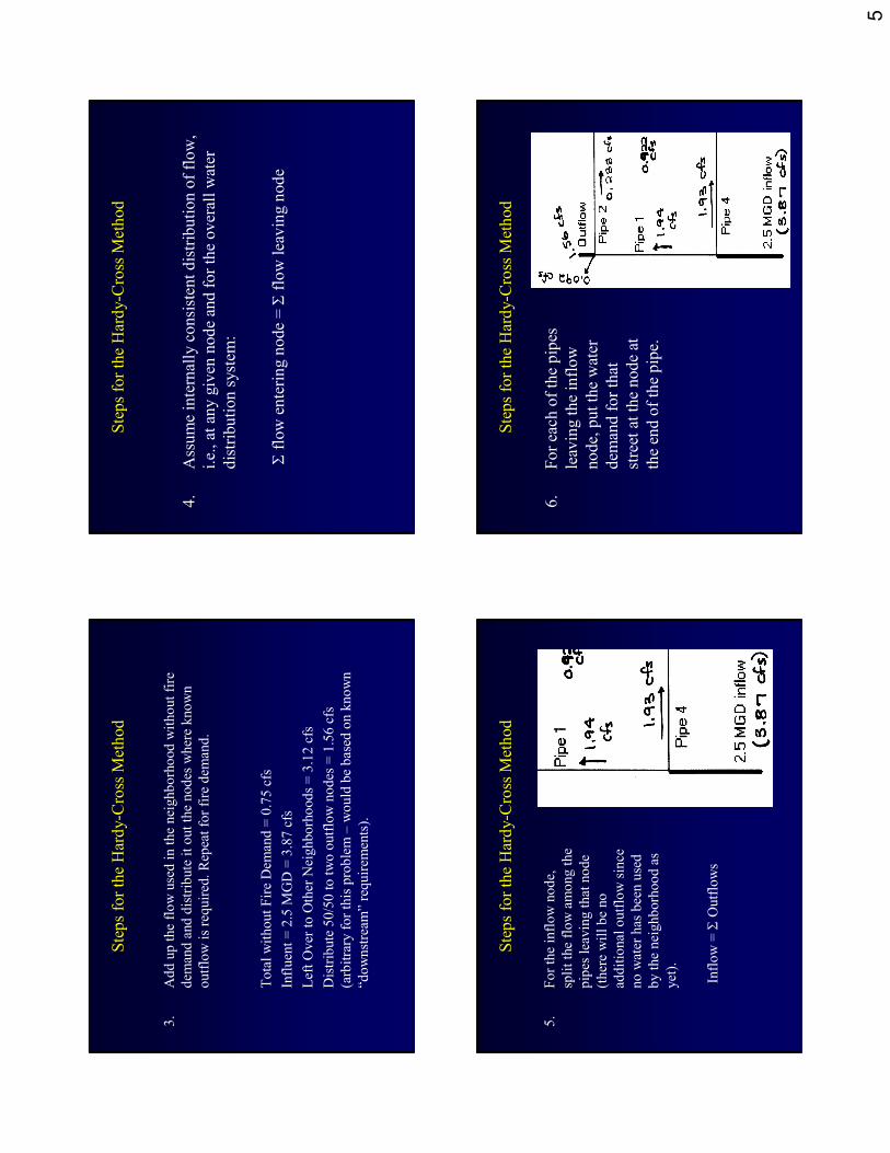
Steps for the Hardy-Cross M
ethod
3.
Add up the flow used in the neighborhood without fire
dem
and and distribute it out the nodes where known
outflow is required. Repeat for fire dem
and.
Total without Fire Dem
and = 0.75 cfs
Influent = 2.5 M
GD = 3.87 cfs
Left Over to Other Neighborhoods = 3.12 cfs
Distribute 50/50 to two outflow nodes = 1.56 cfs
(arbitrary for this problem –
would be based on known
“downstream
”requirem
ents).
Steps for the Hardy-Cross M
ethod
4.
Assume internally consistent distribution of flow,
i.e., at any given node and for the overall water
distribution system
:
Σflow entering node = Σ
flow leaving node
Steps for the Hardy-Cross M
ethod
5.
For the inflow node,
split the flow among the
pipes leaving that node
(there will be no
additional outflow since
no water has been used
by the neighborhood as
yet).
Inflow = Σ
Outflows
Steps for the Hardy-Cross M
ethod
6.
For each of the pipes
leaving the inflow
node, put the water
dem
and for that
street at the node at
the end of the pipe.
6
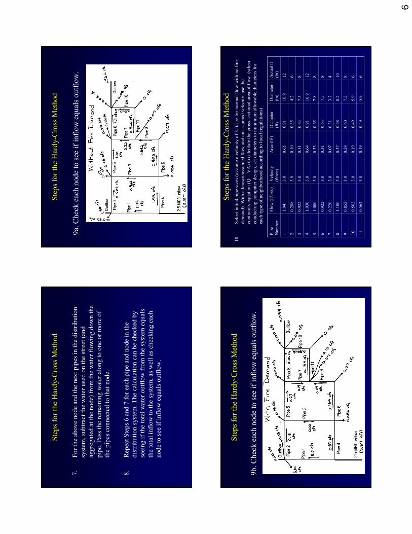
Steps for the Hardy-Cross M
ethod
7.
For the above node and the next pipes in the distribution
system
, subtract the water used on the street (and
aggregated at the node) from the water flowing down the
pipe. Pass the remaining water along to one or more of
the pipes connected to that node.
8.
Repeat Steps 6 and 7 for each pipe and node in the
distribution system. The calculation can be checked by
seeing if the total water outflow from the system equals
the total inflow to the system, as well as checking each
node to see if inflow equals outflow.
Steps for the Hardy-Cross M
ethod
9a. Check each node to see if inflow equals outflow.
Steps for the Hardy-Cross M
ethod
9b. Check each node to see if inflow equals outflow.
Steps for the Hardy-Cross M
ethod
10.
Select initial pipe sizes (assume a velocity of 3 ft/sec for norm
al flow with no fire
dem
and). W
ith a known/assumed flow and an assumed velocity, use the
continuity equation (Q = VA) to calculate the cross-sectional area of flow. (w
hen
conducting computer design, set diameters to m
inim
um allowable diameters for
each type of neighborhood according to local regulations)
5.9
5.9
7.2
8.2
3.7
7.5
7.8
10.9
7.5
4.2
10.9
Diameter
(in)
Actual D
(in)
Area (ft2)
60.49
0.19
3.0
0.562
11
60.49
0.19
3.0
0.562
10
80.60
0.28
3.0
0.852
9
10
0.68
0.37
3.0
1.100
8
40.31
0.07
3.0
0.220
7
80.63
0.31
3.0
0.922
6
80.65
0.33
3.0
1.000
5
12
0.91
0.64
3.0
1.930
4
80.63
0.31
3.0
0.922
3
60.35
0.10
3.0
0.288
2
12
0.91
0.65
3.0
1.94
1
Diameter
(ft)
Velocity
(ft/sec)
Flow (ft3/sec)
Pipe
Number
7
Steps for the Hardy-Cross M
ethod
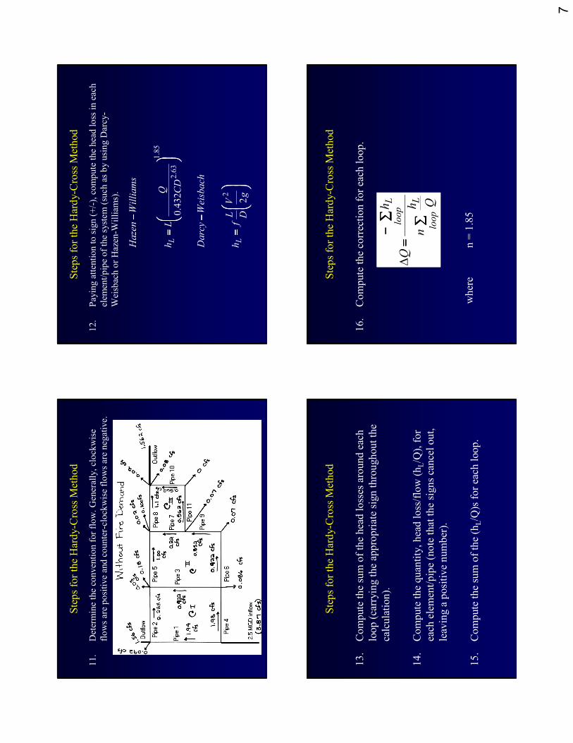
11.
Determine the convention for flow. Generally, clockwise
flows are positive and counter-clockwise flows are negative.
Steps for the Hardy-Cross M
ethod
12.
Paying attention to sign (+/-), compute the head loss in each
elem
ent/pipe of the system (such as by using Darcy-
Weisbach or Hazen-W
illiam
s).
= ===
− −−−
= ===
− −−−
g
V
DLf
h
Weisbach
Darcy
CD
QL
h
Williams
Hazen
LL
2
432
.0
2
85
.1
63
.2
Steps for the Hardy-Cross M
ethod
13.
Compute the sum of the head losses around each
loop (carrying the appropriate sign throughout the
calculation).
14.
Compute the quantity, head loss/flow (hL/Q), for
each element/pipe (note that the signs cancel out,
leaving a positive number).
15.
Compute the sum of the (h
L/Q)sfor each loop.
Steps for the Hardy-Cross M
ethod
16.
Compute the correction for each loop.
where
n = 1.85
∑ ∑∑∑∑ ∑∑∑− −−−
= ===
loop
L
loopL Qh
n
h
Q∆
8
Steps for the Hardy-Cross M
ethod
17.
Apply the correction for each pipe in the loop that is
not shared with another loop.
Q1= Q
0+ ∆Q
18.
For those pipes that are shared, apply the following
correction equation (continuing to carry all the
appropriate signs on the flow):
Q1= Q
0+ ∆Q
loopin–∆Q
shared
loop
Steps for the Hardy-Cross M
ethod
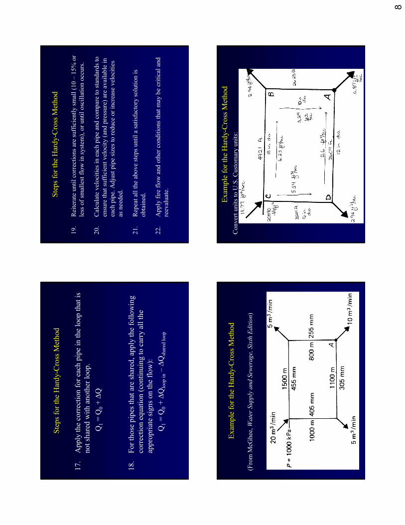
19.
Reiterate until corrections are sufficiently small (10 –15% or
less of sm
allest flow in system), or until oscillation occurs.
20.
Calculate velocities in each pipe and compare to standards to
ensure that sufficient velocity (and pressure) are available in
each pipe. Adjust pipe sizes to reduce or increase velocities
as needed.
21.
Repeat all the above steps until a satisfactory solution is
obtained.
22.
Apply fire flow and other conditions that m
ay be critical and
reevaluate.
Exam
ple for the Hardy-Cross M
ethod
(From M
cGhee, Water Supply and Sewerage, Sixth Edition)
Exam
ple for the Hardy-Cross M
ethod
Convert units to U.S. Customary units:

9
Exam
ple for the Hardy-Cross M
ethod
•Insert data into spreadsheet for Hardy-Cross (solve using
Hazen-W
illiam
s).
•ASSUME: Pipes are 20-year old cast iron, so C = 100.
3.29
10
2625
AB
-2.6
12
3609
DA
-5.54
16
3281
CD
6.23
18
4921
BC
Flow
0(ft3/sec)
Pipe Diameter
(in)
Pipe Length (ft)
Pipe Section
Steps for the Hardy-Cross M
ethod
•Paying attention to sign (+/-), compute the head loss in each
elem
ent/pipe of the system by using Hazen-W
illiam
s (check
that the sign for the head loss is the same as the sign for the
flow).
85
.1
63
.2
432
.0
=
−
CD
QL
h
Williams
Hazen
L
Exam
ple for the Hardy-Cross M
ethod
•Calculate head loss using Hazen-W
illiam
s.
3.29
-2.6
-5.54
6.23
Flow
0(ft3/sec)
54.39
10
2625
AB
-19.93
12
3609
DA
-18.11
16
3281
CD
19.03
18
4921
BC
hL(ft)
Pipe Diameter
(in)
Pipe Length
(ft)
Pipe
Section
Exam
ple for the Hardy-Cross M
ethod
•Calculate h
L/Q for each pipe (all of these ratios have
positive signs, as the negative values for hLand Q
cancel out).
16.53
54.39
3.29
AB
7.66
-19.93
-2.6
DA
3.27
-18.11
-5.54
CD
3.05
19.03
6.23
BC
hL/Q (sec/ft2)
hL(ft)
Flow
0(ft3/sec)
Pipe Section

10
Exam
ple for the Hardy-Cross M
ethod
•Calculate head loss using Hazen-W
illiam
s and column totals:
16.53
54.39
AB
Σ(h
L/Q) = 30.51
ΣhL= 35.38
7.66
-19.93
DA
3.27
-18.11
CD
3.05
19.03
BC
hL/Q (sec/ft2)
hL(ft)
Pipe Section
Exam
ple for the Hardy-Cross M
ethod
•Calculate the correction factor for each pipe in the loop.
where n = 1.85
∑ ∑∑∑∑ ∑∑∑− −−−
= ===
loop
L
loopL Qh
n
h
Q∆
= -(35.38)/1.85(30.51) = -0.627
Exam
ple for the Hardy-Cross M
ethod
•Calculate the new
flows for each pipe using the following
equation:
Q1= Q
0+ ∆Q
2.66
-0.627
3.29
AB
-3.23
-0.627
-2.6
DA
-6.17
-0.627
-5.54
CD
5.60
-0.627
6.23
BC
Flow
1(ft3/sec)
∆Q (ft3/sec)
Flow
0(ft3/sec)
Pipe Section
Exam
ple for the Hardy-Cross M
ethod
HA
RD
Y C
RO
SS
ME
TH
OD
FO
R W
AT
ER
SU
PP
LY
DIS
TR
IBU
TIO
N
Tri
al
I
Pipe Section
Pipe Length
(ft)
Pipe Diameter
(in)
Flow
0
(ft3/sec)
HL (ft)
HL/Q
(sec/ft2)
nΣ(H
L/Q)
(sec/ft2)
Σ(H
L) (ft)
∆Q (ft3/sec)
Flow
1
(ft3/sec)
BC
4921
18
6.2
19.03
3.05
-0.627
5.60
CD
3281
16
-5.5
-18.11
3.27
-0.627
-6.17
DA
3609
12
-2.6
-19.93
7.66
-0.627
-3.23
BA
2625
10
3.3
54.39
16.53
-0.627
2.66
Tri
al
2
Pipe Section
Pipe Length
(ft)
Pipe Diameter
(in)
Flow
1
(ft3/sec)
HL (ft)
HL/Q
(sec/ft2)
nΣ(H
L/Q)
(sec/ft2)
Σ(H
L) (ft)
∆Q (ft3/sec)
Flow
2
(ft3/sec)
BC
4921
18
5.60
15.64
2.79
-0.012
5.59
CD
3281
16
-6.17
-22.08
3.58
-0.012
-6.18
DA
3609
12
-3.23
-29.71
9.21
-0.012
-3.24
BA
2625
10
2.66
36.79
13.81
-0.012
2.65
Tri
al
3
Pipe Section
Pipe Length
(ft)
Pipe Diameter
(in)
Flow
2
(ft3/sec)
HL (ft)
HL/Q
(sec/ft2)
nΣ(H
L/Q)
(sec/ft2)
Σ(H
L) (ft)
∆Q (ft3/sec)
Flow
3
(ft3/sec)
BC
4921
18
5.59
15.58
2.79
0.000
5.59
CD
3281
16
-6.18
-22.16
3.59
0.000
-6.18
DA
3609
12
-3.24
-29.91
9.24
0.000
-3.24
BA
2625
10
2.65
36.49
13.76
0.000
2.65
54.34
0.00
56.46
35.38
54.38
0.64
11
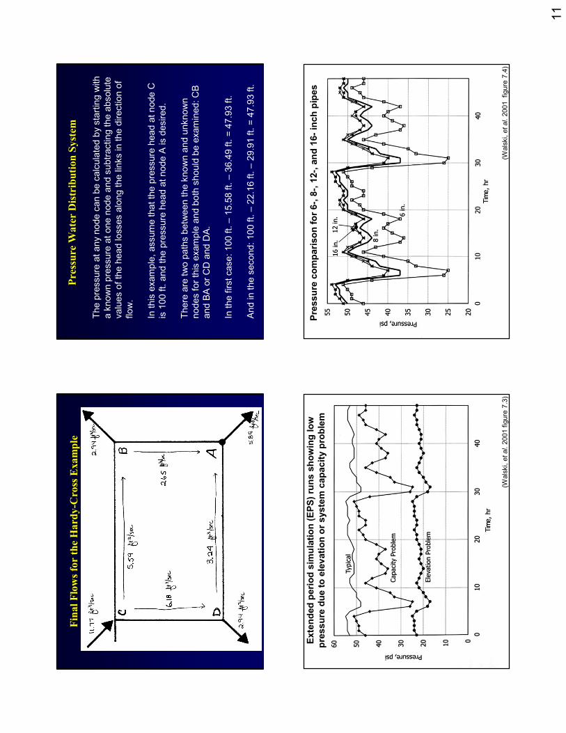
Final Flows for the Hardy-Cross Example
Pressure Water Distribution System
The pressure at any node can be calculated by starting with
a known pressure at one node and subtracting the absolute
values of the head losses along the links in the direction of
flow.
In this example, assume that the pressure head at node C
is 100 ft. and the pressure head at node A is desired.
There are two paths between the known and unknown
nodes for this example and both should be examined: CB
and BA or CD and DA.
In the first case: 100 ft. –15.58 ft. –36.49 ft. = 47.93 ft.
And in the second: 100 ft. –22.16 ft. –29.91 ft. = 47.93 ft.
Exte
nd
ed
peri
od
sim
ula
tio
n (
EP
S)
run
s s
ho
win
g lo
w
pre
ssu
re d
ue t
o e
lev
ati
on
or
syste
m c
ap
acit
y p
rob
lem
(Walski, et al.2001 figure 7.3)
Pre
ssu
re c
om
pari
so
n f
or
6-,
8-,
12-,
an
d 1
6-
inch
pip
es
(Walski, et al.2001 figure 7.4)
12
Head
lo
ss c
om
pari
so
n f
or
6-,
8-,
12-,
an
d 1
6-
inch
pip
es
(Walski, et al.2001 figure 7.5)
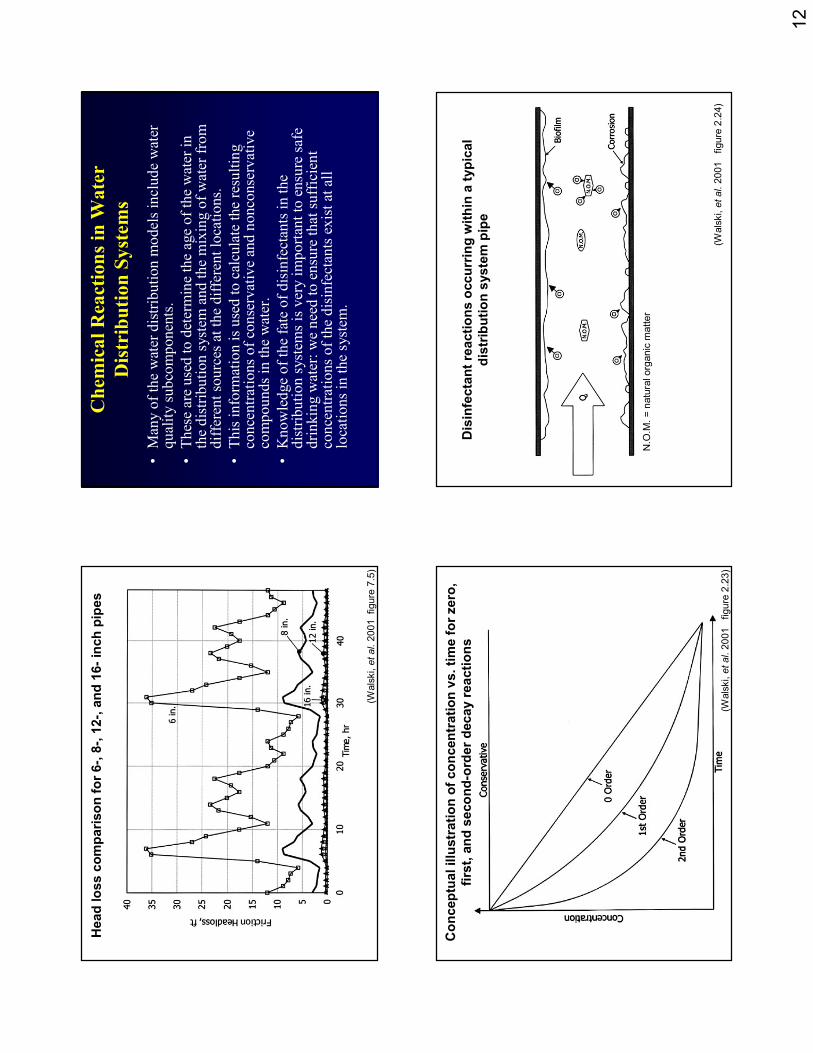
Chemical Reactions in Water
Distribution Systems
•Many of the water distribution m
odels include water
quality subcomponents.
•These are used to determine the age of the water in
the distribution system
and the mixing of water from
different sources at the different locations.
•This inform
ation is used to calculate the resulting
concentrations of conservative and nonconservative
compounds in the water.
•Knowledge of the fate of disinfectants in the
distribution system
s is very important to ensure safe
drinking water: we need to ensure that sufficient
concentrations of the disinfectants exist at all
locations in the system
.
Co
ncep
tual illu
str
ati
on
of
co
ncen
trati
on
vs. ti
me f
or
zero
,
firs
t, a
nd
seco
nd
-ord
er
decay r
ea
cti
on
s
(Walski, et al. 2001 figure 2.23)
Dis
infe
cta
nt
reacti
on
s o
ccu
rrin
g w
ith
in a
typ
ical
dis
trib
uti
on
syste
m p
ipe
N.O.M. = natural organic matter
(Walski, et al.2001 figure 2.24)
13
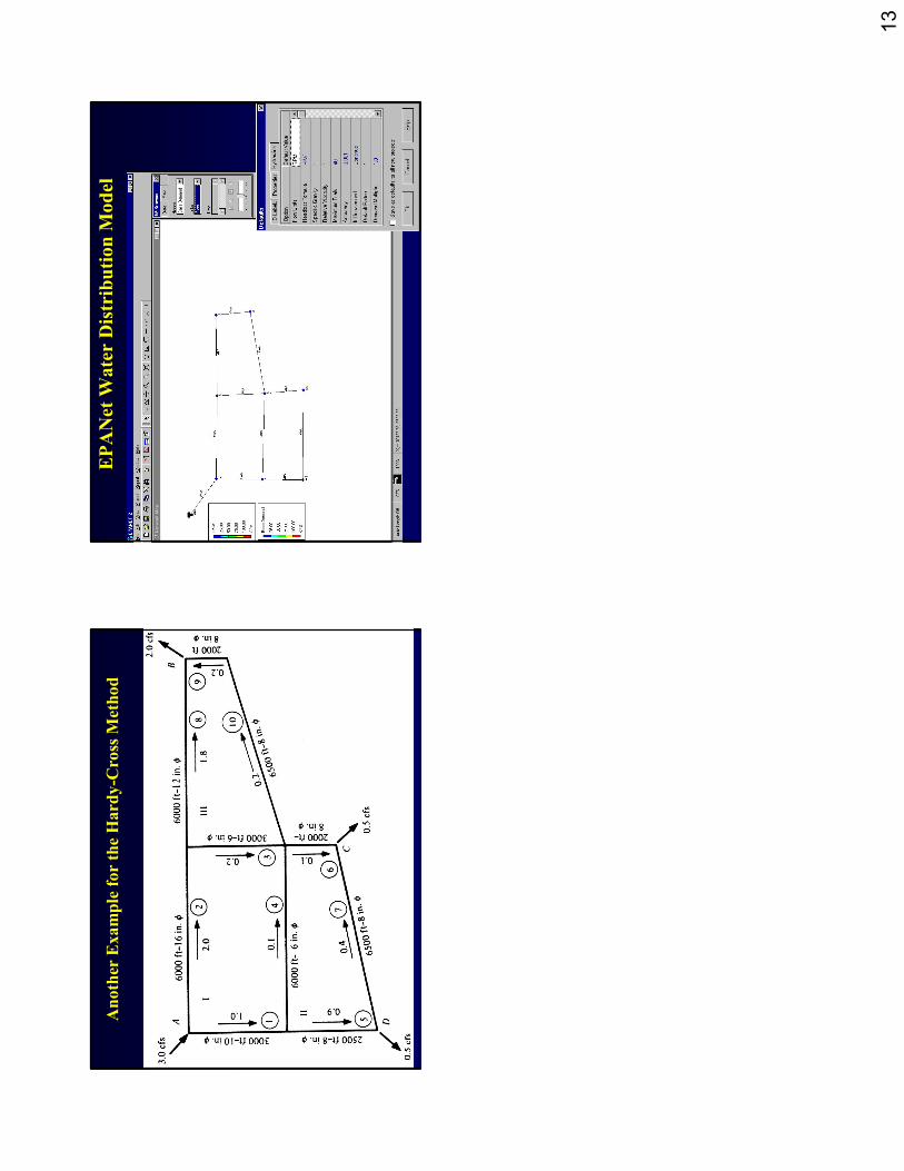
Another Example for the Hardy-Cross Method
EPANetWater Distribution Model


![homepages.inf.ed.ac.ukhomepages.inf.ed.ac.uk/rbf/CAVIAR/PAPERS/TrueVision14...2005-07-25 · begin 644 truevisi.pdf m)5!$1btq+c,*)3e\n7ki_.@t,3&"c(@,"!o8fh*/#p@+tqe;f=t:"`q(#`@ m4b`o1fel=&5r("]&;&%t941e8v]d92`^/@is=')e86t*>-j]7=mr6\eu?>^o](https://img.pdfslide.us/doc/110x75/5b1ea7de7f8b9a22028bd456/-begin-644-truevisipdf-m51btqc3en7kit3ftq.jpg)