Embed Size (px)
Citation preview

—.
m..,,.-7
*., .
%
FOR AERONAUTICS
FLAT
TECHNICAL MEMORANDUM 1369
PLATE CASCADES AT
By Rashad M. El
SUPERSONIC
Translation of “Ebene Plattengitterbei herscha.llgeschwtidigkeit.”Mitteilungen aus dem InstitutfilzAerodynamic
an der E.T.H., no. 19, 1952 ,
..
Washington
May 1956
1

lK
.
.,=.
w
CONTENTS
Page
.
PRE3’ACE. . . . . . . . . . . . . . . . . . . . . . . . . . . . .. iii
INTRODUCTION . . . . . . . . . . . . . . . . . . . . . . . . . ..1
CHAPTER 1. THE FLA!lPlate . . . . . . . . . . . . . . . . . .1. General Considerations . Stiptitions . . . . . . . . . .2. Conditions at Expsnsion Around a Cor-ner . . . , . . . . .3. Conditions of Oblique Compression Shock . . . . . . . . .4. Lift andDrsg of an Infinitely Thin Plate (Exact Solution)5. Lift andDrag atHighMachNumbers . . . . . . . . . . . .6. Calculation of Lift andDrsg by Linearized Theory . . . .7. Comparison of the Results of the Linearized Theory
WithThse oftheExactMethod . . . . . . . . . . . . .
. . 4
. . :
. .
. . 8
. . 10
.* 13● . 15
. . 18
CHAPTER 11. ~ECTION, OVERTAKING AND REl?L31CTIONOFCOMPRESSIONSHOCKS ANDEXJ?ANSION WAW . . . . . . . . . . . . . 19l. Introduction. . . . . . . . . . . . . . . . . . . . . . . , . 192. Small Variations. . . . . . . . . . . . . . . . . . . . . . . 193. Overtaking of Compression Shock and Expsnsion Wave . . . . . . 224. Intersection of Compression Shock and Expansion Wav-e. . . . . 265. Crossing ofExpsnsionWaves . . . . . . . . . . . . . . . . . 316. Reflection of Compression Shocks and Expansion Waves . . . . . 33
CHAYTER 111. THE CASCADEl?ROELE&f. . . . . . . . . . . . . . . . . 34l.~oblem . . . . . . . . . . . . . . . . . . . . . . . . . . . 342. Method ofCalctiation . . . . . . . . . . . . . , . . , . . , 343.-le . . . . . . . . . . . . . . . . . . . . . . . . . . . 354. Calculation of Thrust, Tangential Force and Efficiency . . . . 37
cHAPrERIv. UNMRU3D CASCADE THEORY . . . . . . . . . . . . . . 4.0l.lksumptions . . . . . . . . . . . . . . . . . . . . . . . . . @2. Linearization of Cascade problem . . . . . . . . .. . . . . . . 403. CalculationofLift sudDreg . . . . . . . . . . . . . . . . . 41k. NumericalExsmple . . . . . . . . . . . . . . . . . . . . . . 445. ComparisonWith Exact Method . . . . . . . . . . . . . . . . . 45
Cmwrm v. SCHLIEREN PIK)TOGRAPHSOFCNCADE ITOW. . . . . . . . . 46l. Cascade Geometry. . . . . . . . . . . . . . . . . . . . . . . 462. Experimental Setup. . . . . . . . . . . . . . . . . . . . . . 473. SchlierenPhotographs . . . . . . . . . . . . . . . . . . . . 47
CHAFTERVI. THE FIAT PLATE CASCADE AT SUDDEN ANGLE-OF-ATTACKCHANGE . . . . . . . . . . . . . . . . . . . . . . . . . . . . . 49l. problem . . . . . . . . . . . . . . . . . . . . . . . . , . . 492. TheUnsteadySource . . . . . . . . . . . . . . . . . . . . . 50
i
.
3. Rressure and Velocity of a Periodically ArisingSource Distribution. . .“. . . . . . . . . . .
4. Single Flat Plate in a Vertical.Gust (Biot 1945)~. The Straight Cascade . . . . . . . . . . . . . .6. Numerica~Exsmple . . . . . . . . . . . . . . . .
CHAPTER VII. EJWICIENCY OF A SUPERSONIC PROPELLER . .l.htroduction . . . . . . . . . . . . . . .2. Effect of lZrictionon Cascade Efficiency .3. Effect of Thickness . . . .
of the Efficiency. . . . . . . .of a Supersonic
SUMMARY. .
REFEmNcEs .
!I!ABLEs. . .
FIGURES . .
.
.
.
.
.
.
.
.
. .
. .
. .
. .
.
.
.
.
.
.
.
.
.
.
●
✎
.
.
.
.
.
.
.
.
.
.
.
,
.
.
#
4
.
.
.
.
.
.
,
.
,
●
✎
●
.
.
.
.
. .
. .
. .
. .
,
.
.
#
. . .
. . .
. . .
.
.
.
.
.
.,.
.
.
.
.
.
.
.,
Propeller
.
.
.
.
,.
. .
. .
. .
,
.
.
,
.
.
.
.
.
.
.
.
.
.
.
.
.
.
.
.
.
.
.
.
.
.
.
.
.
.
.
.
.
.
.
.
.
.
.
.
.
.
.
.
.
.
.
.
.
.
.
.
.
.
.
.
.
.
.
.
52596167
~172
;
77
78
79
91
“w
ii
PREFACE
The work on the present report was carried out at the Institute forAerodynamics of the E.T.H., Z&ich, under the direction of Prof.Dr. Ackeret, during the time from December 1949 to June 1951.
I want to express here my deep gratitude to.Prof. Ackeret for hissuggestions and for the great interest he took in my work.
I em very grateful to Dip~.-Eng. B. Chaix, scientific assistant atthe Institute, and to Mr. E. Hurlimann, precision mechanic, for theirindispensablehelp in tsking the schlieren pictures.
I should like to acknowledge that the “Faruk Diversity”, Alexandria(Egypt) made my studies in Zfiick possible.
.
iii
NATIONAL ADVISORY COMMITTEE FOR AERONAUTICS
TECHNICAL M1310RAND~ 1369
m PLATE CASCADRAT SUPERSONIC
By Rashad M. El Badrawy
INTRODUCTION
sPEE@
The cascade problem in the subsonic range can be analyzed undercertain assumptions either by mapping or substitution of the blades bysingularities - sources, sinks snd bound vortices - where the separationof flow from the blades can cause various departures from the obtainedresults.
Raising the flow velocity to a given value is accompanied by sonicvelocity within the cascade, which usually renders the solution of theproblem even more difficult. The sane complication exists on the cascadein flow at supersonic speed, in which the velocity is retarded to sub-sonic by shocks.
But when the cascade operates entirely in the supersonic range, theconditions become clearer. All disturbances act downstream only from thesomces of disturbance, so that the pressures and velocities at the sur-face of a sufficiently thin airfoil in the stremn csnbe readily determhed.
The present report deals exclusivdy with problems of cascade flowin the supersonic range. As is known the flat infinitely thin plate isthe best airfoil with respect to wave resistance in supersonic flows;hence it is logical to start with the cascade of flat plates. The lastchspter deals with the case of finite thickness.
Lift and wave resistance of an isolated plate are computed firstsince the cascade -problemcan often be reduced to”this special case.The well-known theories of two-dimensional.supersonic flow are applied -that is, the laws of oblique compression shocks and the exps.nsionarounda corner.
The air forces are then calculated again and compsxed with the pre-viously obtained exact values by meam of Ackeret’s formulas of line=izedtheory.
*“Ebene Plattengitter bei herschallgeschwindigkeit.” Mitteilungenaus dem Institut ffi Aerodynamic an der E.T.H., no. 19, 1952.
2 NACA w 1369
The cascade problem was to be solved in such a way as to be free.
from the inevitable inaccuracies of the graphical method. For this reasonthe cases of overtaking, crossing and reflection of compression shocks and W“expansion waves frequently occurring on supersonic cascade flows, whichusually are solved by graphical method, are analyzed in chapter 11.
In chapter 111 the cascade problem is discussed and its solutiondescribed in the light of the results obtained in chapter II. A numericalexample is also given. The same chapter gives further a definition ofthe efficiency of the simple supersonic cascade and an evaluation forseveral angles of stagger and attack.
The small angles of attack involved justified the use of a linearizedcascade theory.l This is done in chapter IV. The numerical example ofchapter III is thus linearized and the results compared with those of theexact solution. The supersonic cascade flow at various singlesof attackwas recorded by schlieren photographs of the flow between two parallelplates, in the high-speed wind tunnel of the Institute (chapter V).
Chapter VI deals with the specific case of unsteady flow throughthe cascade, caused by abrupt angle-of-attack changes.
w
lAccording to Ackert’s linearized theory, the lift and drag ofdouble-wedge profile of thickness d and chord Z at angle ~ insonic flow M is, in the presence of fii.ction(cf)
1- 7
For the best bag-lift ratio ~ = ~,
the wave resistance should be equal to theness effect. In that event
put $& = o. This means
sum of friction drag and
-..
1
+ Zcf K“4
.opt=2,0pt=L’/-
asuper-
G
that
thick-
P
Assuming possible values for d/Z and cf results in comparatively -G
small optimum anQes vopt.
v
NACA TM 1369 3
.
In chapter VIZ the effect of friction and thickness in a special
* case on the cascade efficiency is analyzed. Since there might be apossible application of the supersonic cascade to the supersonic pro-peller, a simple evaluation of the efficiency of such a prope~er ismade. A parallel steady two-dimensional flow is - with exception ofchapter VI - postulated.
The conventional notation is used unless specifically stated otherwise in the text.

4 NACA TM 1569
CHAPTER I. TKE FLAT
1. General Considerations -
The general equation of continuity of
ME
Stipulations
any compressible flow is
ap+ a(pu) + a(pv) ;M=o——at ax by az
(1)
The rate of propagation of a small disturbance, that is, the sonicvelocity, is, as is known
(2)
Cpwhere K = q“
In flows, in whichtion can be written as
a flow potential p exists, the continuity equa- J
The momentum theorem gives the following relations
1
-Q Q=a+afi+afi+a *“pax bat Z3xaxz baxay azaxaz
(4)
,
2KNACA TM 1369 5
.
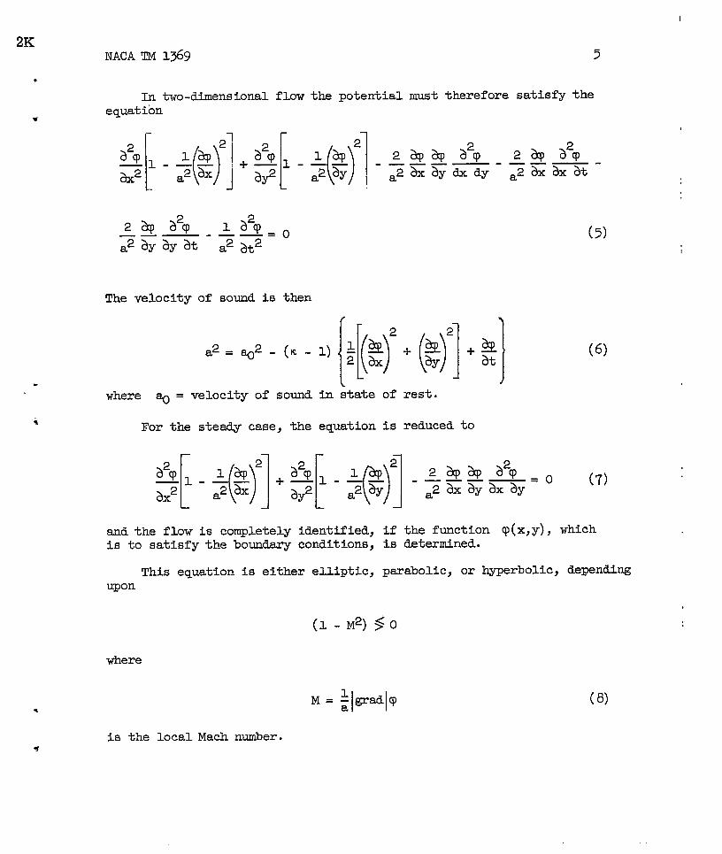
In two-dimensional flow the potential must therefore satisfy theequation*
The velocity of sound is then
a2=%2(K-1)[,~y+& r]+3]
where % = velocity of sound in state of rest.
i For the steady case, the equation is reduced to
(5)
(6)
and the flow is completely identified,is to satisfy the boundary conditions,
This equation is either elliptic,upon
if the function q(x,y), whichis determined.
parabolic, or hyperbolic, depending
(1- M2)$0
where
(8)
is the local Mach number.●

6 NACA TM 1369
.
The use of this equation is difficult if its type in the particularrange, as in the transonic rsmge, is changed. However, the flows analyzed .here, are of identical character everywhere, that is, the flow is of thehyperbolic type.
One of the known solutions is the expansion around a corner, developedby Prandtl and Meyer (ref. 1).
2. Conditions at Expansion Around a Corner
The two-dimensional flow past the wall AE at a Mach number Ml
(fig. 1) is deflected by a convex bend at E through an angle @, throughwhich an expansion is initiated. Thespreads out solely in the range lying
where
disturbance proceeding from Edownstream of the Mach line EBl,
and stops at
+ BIEA’ = Mach angle l-q= sin-l ,&Ml
the Mach line EB2, where
4B2ED=v2= sin-1-$
(9)
In it M2 is the Mach number of the flow after the expansion.
The streamlines in range B1EB2 are curved similarly and run
parallel to the wall ED downstream of this range.
It can be proved that the Mach lines in this flow are the character-istics of the differential equation which define the potential.
When the expansion
the following relations
proceeds from
can be proved
tanp2=A
a Mach number Ml = 1, (Ill= ;)9
(ref. 2):
cot h (lo)
.
w
NACA TM 1369 7
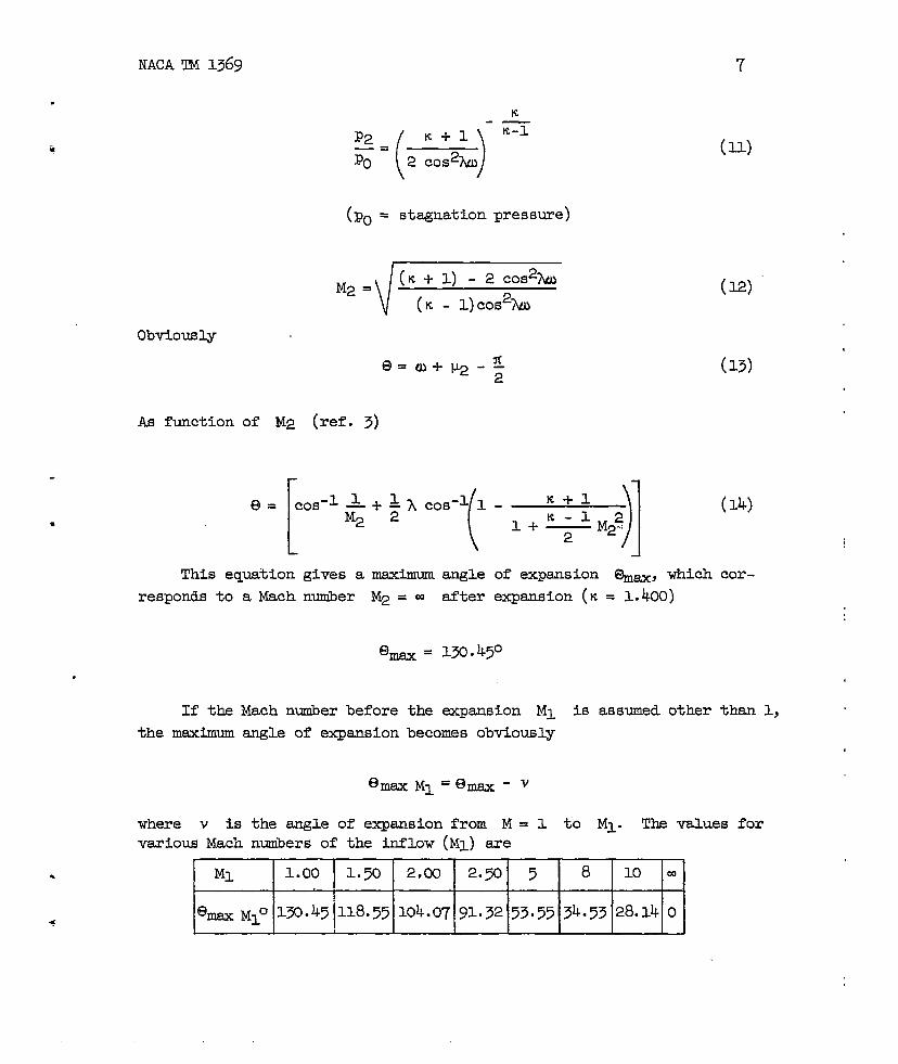
K.—
Pa
()
K+l K-1—=Po 2 Cos%
(11)
(Po = stagnation pressure)
M2 =
d
(K + 1) -2 Cos%u
(K - 1)cos2Xo.)(L2)
Obviously
(13)e= cD+ l+-
As function of M2 (ref. 3)
.
(14)
which cor-
1c
This equation gives a maximum of expansion &,angle
afterresponds to expsasiona Mach nuder M2 = M
Elm =
(K = 1.400)
lx. 450
,
expansion Ml is assumed other than 1,If the
the maximum
Mach number before
angle of expansion
the
becomes obviously
where v is the angle of expansion from M = 1 to Ml. The values forvarious Mach nwibers of the inflow (MI) are
Ml 1.00 1.X 2pm 2.X 5 8 10 m
o 130.45 118.5Y 104 ● 07 91.32 53.55 34.53 28.14 0%sx Ml

NACA TM 1369
3. Conditions of Oblique Compression Shock
The di.scontinuitiesthat may appear in supersonic flows and acrosswhich velocity, pressure, density, temperature, and entropy undergo adiscontinuity, while the total energy, thermic and mechanical, remainsconstant, were predictedby Riemann (1%0) and Rankine and Hugoniot’(1887)as normal compression shocks.
.
—..
In oblique shocks (Prandtl-Meyer)only the velocity component normalto the shock front is modified.
In figure 2 the supersonic flow past the wall AH is deflected at Eby an angle 8. A compression shock is produced and the shock front ESiS inclined at an angle 7 - the shock angle - to~d the air flowdirection.
—
With’subscript 1 denoting the state before the shock and subscript 2that after the shock it canbe proved that (refs. 3 andk)
Pa‘—=( )
~M12sin27 - &PI (15) .
1
+{
K-1P2’ ~.lPl F 2
(K :’1)2 ( )[
sin27- H 1+ 4K
]( )-]
‘1 KPo‘=’+1~
sin2y —fc+l (K - 1)2 ml
(‘+-1 M12Cotb= —
2)
-ltanyM12sin2y - 1
up‘ Cos—= Y~ COS(7- 5)
(16)
(17)
(18)
(19)
NACA TM 1369 9
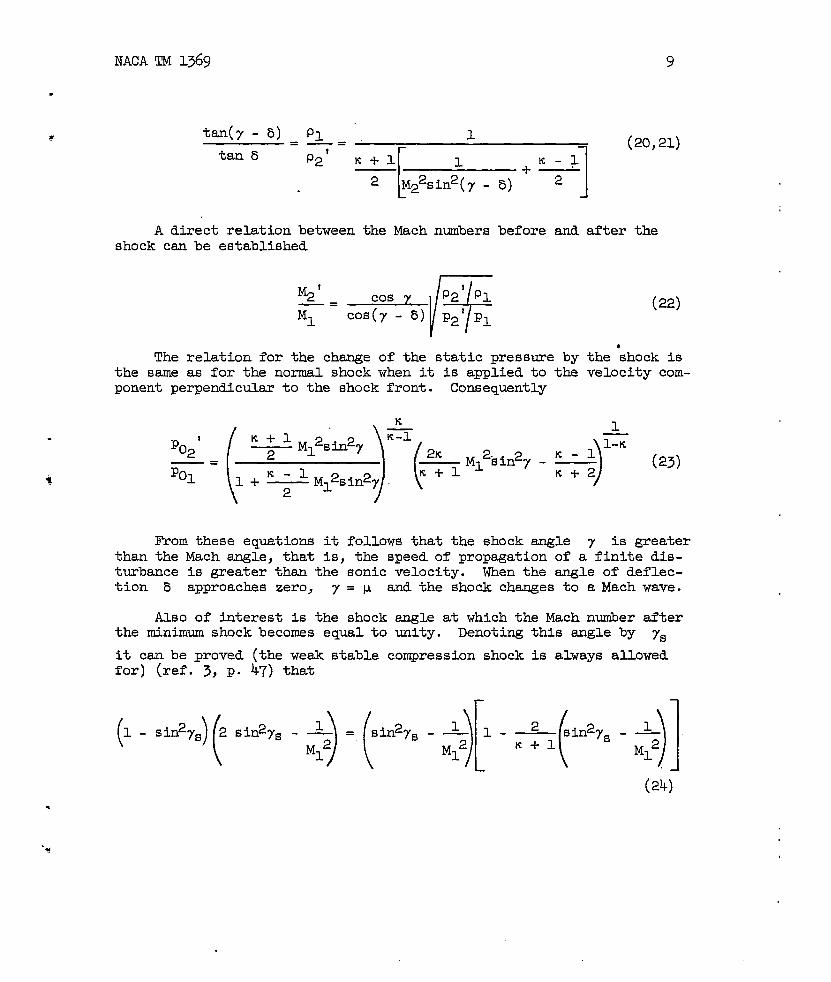
tan(y - (5) P1 1=—=
[
(20,21)tan 5 P’2‘ Ic+l 1 K- 11+-2 M22sin2(y - 5) 2
A direct relation between the Mach numbers before and after theshock can be established
%’ Cos ‘/+P2’ P1—=
‘1 COS(7 - ~) Pa’ P1(22)
The relation for the change of the static pressure by the ‘shockisthe same as for the normal shock when it is applied to the velocity com-ponent perpendicular to the shock front. Consequently
K# \— 1
2=(17y5J7*M’sin27-that the shock angle 7
(23)
is greaterFrom these equations it followsthan the Mach single,that is, the speed of propagation of a-finite dis-turbance is greater than the sonic velocity. When the am.gleof deflec-tion b approaches zero, 7 . w and the shock chsmges to a Mach wave.
Also of hterest is the shock angle at which the Mach nuniberafterthe minimum shock becomes equal to unity. Denoting this angle by 7~
it can be proved (the weak stable compression shock is always allowedfor) (ref. 3, p. 47) that
(24)

10 NACA TM 1369
This equation is used to determine the msximum shock angle whichcorresponds to a Mach number before the shock Ml = w and a Mach num-
ber M2’ = 1 after the shock. The result is
K+lsin2ys = — .
2ti
hence
(25)
7s = 67.EP
at~= 1.400 (air).
By”equation (18) the correspondingdeflection angle 5s is
65= 45.5W
2Table 1 and figwe 3 represent the values of ~s and bs at
various Mach numbers Ml.
4. Lift and Drag of an Inftiitely Thin Plate (Exact Solution)
An infinitely thin plate ab in parallel flow at supersonic veloc-ity U1 is placed at the angle ~. It is assumed that the width of the
plate transverse to the flow direction is M, so that the problem is twodimensional.
The streamlines above oa (fig. 4) experience a deflection whichis associated with an expansion. So the state at the upper side of theplate canbe definedby equations (10) to (14). But below the plate acompression shock ad occurs. The state of the flow on the lower sideof the plate is accordingly determined from the formulas (16) to (21).
The force on the plate per unit area is
K=(P2‘ - P2
)(26)
2The weak stable shock is always taken into account. See Richter,
ZAl@f,1948 and Thomas, prOC. N.A. Se., NOV. 1948.
NACATM 1369 11
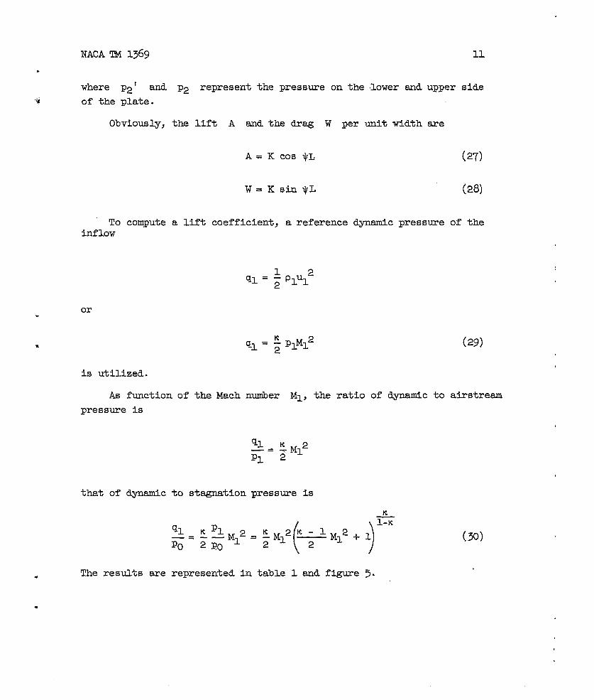
.
where P2’ and- P2 represent the pressure on the lower and upper side
‘i of the plate.
Obviously, the lift A and the drag W per unit width are
A= K COS IJL (27)
v= K SillWL (28)
To compute a lift coefficient, a reference dynamic pressure of theinflow
or.
. (29)
is utilized.
As function of the Mach number Ml, the ratio of dynatic to airstream
pressure is
that of dynamic to stagnation pressure is
* The results are represented in table 1 and figure 5.
.
(30)

12 NACA ~ 1369
Lift snd drag coefficients are herewith
or, if
A P2‘ - P2Ca=—= Cos q
qlz ql
w
()
P2: - P2c~ = —=, sin *
@ !L~
1
all pressures sze referred1- 1
Ca =
The &?ag/lift ratio is
to stagnation pressurer -1
1]()PJ P2—-—Po Po
%= sinql
q
(31)
(32)
(33)
Table 2 gives the values of Ca, Cw, and e up to Ml = 10 as
computed by the formulas (32) and (33).
In the calculation of the Mach numbers up to Ml = 4, the tables
by Keenan and Kaye (ref. 6) as well as those byFerri (ref. 3) were usedto define ??2/Po ~dP2’lp~ (~=1.~o).
For higher Mach numbers, the formulas of sections 2 and 3 wereemployed. At each Mach number, the angle of attack was varied up to~s(M2’ = 1).
Figures 6 and 7 show the variation of Cw end Ca over the mgle
of attack ~; figure 8 shows the pohrs ca plotted against Cw.
The boundary curves show the maximum lift and drag coefficients that -can be expected without getting in the trensonic range.
#
3KNACATM 1369 13
Other values for the boundsry curve sre given in table 3. Since thepressure distribution on the upper and lower side is constant, the result-ant force is applied at plate center-and is normal to the plate. There isno suction force as in subsonic flow.
~. Lift and Drag at High Mach Numbers
At high Mach numbers the singleof &ttack of the plate can exceedthe ms.ximsunexpansion angle ~ (section 2) corresponding to the Mach
number of the airstream % = *S at MI ~ 6.4). Hence, when assuming
continuous flow, an empty wedge-shaped zone between plate and flow appears.This zone is largest at constant angle of attack when. Ml = =. h that
event, no deflection of flow is possible.
Owing to this vacuum space, the pressure at the upper side is zero.The resultant force K is obtained then from the pressure on the lowerside, behind the compression shock. Hence, per unit area
or, when referred to the
K= P2‘
WC pressure
(34)
of the airstream,
Introducing p2’/pl from equation (15) gives
K 4 -1 2—= Sillzy- ~—ql Ic+l K+1M2
‘1
where the term containing l/M12 can be disregarded
K 4—=— sin27Q K+l
(35)
without great error.
(36)

14
So the lift and drag coefficient are
Ca =
%=
Both formulas are dependentexist the relation given infollows (5 = *):
4 sin2y cos *K+l
1
)
NACA TM 1369
4 sin27 sin.~K+l
J
On Y W ~ only. Between theseequation (18), which can be written
cOt’=(Fsin2;-.
where the term ~ can be disregarded again. Then -Mlz
The values and curves
(37)
thereas
(38)
S.nd
The
designated with M = m in table 2 and figures 6,7 and 8 were defined by equations (37) and (38). For comparison the lift
&ag was also computed by Newton’s formula (the normal component)
correspondingvalues
Ca = 2 sin2* cos
%= 2 sin3~
and curves carry
‘+
1
the subscript N.
(39)
.
“.

NACA TM 1369 15
.
ii
.
.
6. Calculation of Lift and Drag by Linearized Theory
According to Ackert’s linearized theory, the
in~ay
can be disregarded without great error in
members of higher order
the potential equation
1-
for slender bodies at small angles of attack, because the interferenceflows are small compared to that of the airstream.
The equation reads accordingly.
[ ()]&l J?22 +252=0ax2
~2 &ay2
Inserting
()&322@a2 ax
and observing that M is greater than unity, the equation reads
a2q o5(M2-1) -—=
ax2 ay2
The general solution of this equation is
.
.It indicates,potential are
(40)
(41)
as stated in section 2, that the lines of constantthe Mach lines of flow, and theti slope has the Mach angle p.

16 NACA TM 1369
This solution shows further that the flow velocities
U=??i ~. .=32ax hy
satisfy the condition
“=-v+= (42)
At the surface of a body in the stream
u..QXUdx
is applicable.
The pressure variation by the momentum equation reads
4= -U AU=-UU (43)P
where U is flow velocity and u is interferenceflow in stream direc-tion.
Accordingly
(44)
NACA TM 1369
The pressure difference between both sides of a flat plate isG
The lift snd drag coefficients at the angles in question sre
.a. _k4_
F= 1
C“=*I.The drag/lift ratio according to this theory is
%?$E =—=
Cs,
17
(45)
(46)
(47)
Instead of the expansion wave and the compression shock at theleading edge, it has simple Mach lines as interference lines (fig. 9), “in contrast to the exact theory.
The values given in table 4 and plotted in figures 10 snd 11 werecomputed by thes’eformulas. The calculations were carried out at eachMach number up to singleof attack ~s - from the exact theory. The cor-
responding Ca Slld C~ values lie on the curve G’.
At sonic velocity on the lower side of the plate p2’/po = 0.5283.
This value, introduced in the following directly obtainable relation
2*CI1P2‘ -P1=$LP=
m
(48)
18
and
NACA TM 1369
gives the singleof attack ($~z) correspondingto
eral is greater than ~s. .
M2 ‘ = 1, which in gen-
7. Comparison of the Results of the Linearized Theory With
In
ficient
at Mach
It
Those of
table 5, the difference
of the exact method and
numbers Ml = 1.40 and
the
is
cL
Ml
follows that the linearizedfor small angles (up to about 100).
and ~ we too small.
Exact Method
(CG - @, where CG is the coef-
is that of the linearized theory
= ~.oo..
theory is a very good approximationFor greater singlesthe values of Ca
#
In figuxes 6 and 7, the Ca and ~ curves by linearized theory
marked A’ and A me included for comparison.
19NACA TM 1369
CHiPl!ER11. INTEHZC?YON, OVIWUKING ANDREFLEC!lIION
OF COMPBXSSIONSHOCKSANDEXPANSIONWA=
1. Introduction
Overtaking of expansion waves and-compression shocks in supersonicflows occurs when the msrginal streamlines - or boundary walls - changetheir direction twice in the opposite sense (fig. 12(a)).
If expansion waves or compression shocks strike a fixed wall andtheir slope tows.rdthe wall does not exceed a given angle, they arereflected as expansion waves or compression shocks (fig. 12(c)). Crossingsoccur in flows through channels and free jets (fig. 12(b)). All theseevents can occur in cascade flows (fig. 12(d)).
2. Small Variations
(a) Suppose that a small. flow ML PI} al, pl past
expansion is L@. If m istions are permissible.
s
expansion occurs.at B in the supersonicthe walIi AB (fig. 13). The singleof
sufficiently small, differential considera-
Bernoulli’s equation gives
41 = - Plul ml (49)
where U is the magnitude of the velocity and AU its variation; 4 iSthe pressure veriation.
Since the vectorial velocity variation is normal to the interferenceline, the vsriation of U is
(50)

20 NACA TM 1369
hence
“=-F’But, as the dynamic pressure q ,isgiven by
the pressure variation can be written as
The variation of the Mach number M follows at (ref. 3, p. 26)
(51)
(52)
(53)
The Mach line BE1 forms with flow direction AB the Mach angle wl~
the Mach line BE2 at the end of the expansion the Mach line p2. Now
it may be assumed that this small expansion takes place on the inter-ference line BEt, whereby
(54)
(b) A simple differentiationgives the change of the shock angle 7as well as the pressure change .p2’ after the shock, due to a small vari- .
ation of the angle of deflection 5, for the compression shock AB(fig. 14) .
w
iKNACA TM 1369
21
Between 7 and b the relation (eq. 18)
( ).K+1M122
cot 5 = tsa 7 -1
M12sin2y - 1
exists, and therefore
where
A= ~ M122
(B = M12sin27 - 1
)
and
c [() 22Asin2b sec27 ~ - 1 - M12sin 7 —=-
B B2
The pre.s~e P2’ after the shock is (eq. 15)
(2K )
K+lP2‘ =Pl— M12sin27 - ~
K+l
and the result for a small variation of
+ . 2KAp2‘ = P1M12 ~
s
the shock intensity is
sin 27 A7
(55)
(56j
(57)

22 .
3. Overtaking of Compression
NACA TM 1369
.
Shock and Expansion Wave
(a) The supersonic flow Ml, PI, PI past the till
undergoes a directional change b at E. The compressionthe flow direction form the shock angle 71 in zone (1).
sion takes place about an angle Q, and the expansion wavethe compression”shockat F. To simplify the calculation,
All (fig. 15(a)) -
shock EF andAt C an expan-
FCG overtakesthe continuous
expression is replaced by a given n&er-of expansion waves of finiteintensity, whereby a successive expansion through these waves is assured.If n is the number of waves, the expansion due to a wave is @/n= A~.The number n must be so chosen that L@ is sufficiently small.
Now consider the intersecting of wave ~l(f@ m compression
shock EFl(b), figure 15(b).
From F~ the compression shock advsmces with weaker intensity indirection Gl, that is, it deflects the flow less - say by ~~. FIG1 forms
with the flow direction the angle y’ at (l). Indicating the various zonesby (1), (2), (3), and (4), the streamline through F1 splits the zone (4) ~
into the portions (4.) and (~). The flow in (2) and (3) is fully known,because the angles b and A@ are known.
To define the conditions in (4), the streamlines S1, S2, and S3v
are examined. The directional change of S2 amounts to (5 - A@). Butalong S3 the flow experiences the directional change 5’. To maintain
equilibrium in (4), the pressure as well as the velocity direction above~d below the stre&mline- S1
In general, the pressureas from (1) to (4), so that acompression too - must appear
must be equal.
change from (1) toward (3) is not the sanereflected expansion wave - possibly a smallbetween (3) and (4), say along a line FIH1.
Supposing that this reflected wave is an expansion wave of inten-sity A@’. By “intensity” of an expansion wave or a compression shock ismeant the deflection, which the flow experiences in the process.
The pressure in (~) is, (accordingto section 2)
ph=p3f-,_:) (58)

.
NACA TM 1369
The difference
23
of the deflection angles smounts to (5’ - 5) = &. Ingeneral, this intensity decrease is–small,is much stronger than the expansion wave.9shock sngle 7 is A7.
The pressure in (~) follows froIutheHence we can say that
P40 = P2’
This is again the equation for sma~equation (57). Accordingly
p4~ = P2’ - p1M12
POsti~ p40 = P4U, gives.
because the compression shockThe corresponding change in
change in shock intensity.
- &z’ (59)
variations derived for shocks from
2K— Sb 27 A7 (60)K+l
For the velocity direction in zone (4) to be unequivocal, it must
A3=A5+M’ (62)
The relation between shock intensity variation and angle of shock(eq. (55)) together with the two previous equations gives
.J45L( QZQFG ---F
c )

24
.with the constants
‘=*-1
The condition for
NACA TM 1369
(64)
2 M12sin 2y
‘=?
Q=M22 - 1
(
-1M12sin2y - &
)
equality of static pressures is not identical withthat for equality of Vel;city &gnitude above and below the streamline S1.
As the shock losses on either side of the intersectionpoint F areunlike, the stagnation pressures in the wake above and below streamline S1
are different, hence there is a small vortex layer along this streamline.
Fig’we 16 represents the graphical solution of the problem by meansof the characteristicsand the shock polars. The condition for equalitythrough equality of velocity magnitude in the entire zone (4) isapproximated.
(b) The reflected wave is disregarded:
In general, the angle of deflection AE$’- intensity of the reflectedwave - is very small (compare numerical exsmple). Thus the pressure in(3) is not much Unlfie that in (4), so that this reflected wave FIHl can
be discounted.
In this eventor in other words
With equation (~5)of the compression
the flow directions in zones (3) and (4) are identical,
L5 can beshock. The
A@=LX3 (65)
defined and from it the new direction 7’velocities in (3) and (4) have then obvi-
ously the seinedirection but not the same mag~itude b+ reason of the smallvort~x layer developing between (3) and (4).- -

NACATM 1369 25
.
* Free stream:
P1/P()= o.127&2
Before overtaking:
shock intensity
shock angle
hence the state in zone (2)
p2po = 0.1773
intensity of the expansion wave
state in zone (3):
P3/Po = 0.1693
Determination of constants:
Numerical Exemple
Ml = 2.000
5 = 60
7 = 35.24°
M2 = 1.7W
A@= 1°
M3 = 1.818
c = 1.078
F = 3.04G= 3.015.Q= 3.175
Inserted in eq~tion (63) and (64) gives: inte&ity of the reflected wave●
Ay = 0.89°
A@’ = 0.06°
By equation (62)
L5=A@- A@’ = 0.94°
Therefore the shock intensity sfter overtaking is
5 = 3.04°
The new shock angle 1s
Y’ = Y - AY=”34S350
The reflected wave disregarded, leaves
shock titensity
angle of shock
It is readily apparent thatscsrcely affects the pressure in
.
Ay = Cm=cm= L 078°
5’ = 50
Y’ = 34.16°
the reflectedzone (3).
wave is very small, hence

26 NACA TM 1369
4. Intersection of Compression Shock and Expansion Wave
Figure 18(a) represents an expansion wave w of intensity ~proceeding from the corner A. At F this wave crosses a compressionshock of intensity b emanating from the corner B.
As before, the continued expansion is replaced again by n expansionwaves between which the flow is straight. The deflection by each wave is
&=:
After crossing (fig. 18(b)) the compression shock has an intensity 5’and a shock angle y’. Now the expansion wave has the intensity L@’.
The zones produced this way me numibered(l), (2), (3), red(4).The streamline FIS splits the zone (4) into (4.) and (4u).
Looked for now is the shock intensity 5’, shock angle 7’, andexpansion angle &l’ after crossing, and the state of flow in (4), whenthe state of-flow in (1)
According to chapterdetermined directly.
The pressure in (~)to the laws in chapter 11
p41J
5, 7 and- 2@ me &own. ,..
I the state of flow in (2) and (3) can be
follows through a “smallexpansion @r accordingat
(j- ~M12=p21- \Ml’ (66)
\v Ml~ . 1
J
where LW is still unknown.
the
The
The method of solution consists in first making an assumption forshock intensity after intersecting,which is
corresponding
5~= (b-L@
angle of shock would be 7i.
(67)

NACA TM 1369
The state after this
according to chapter II.
27
shock, indicated by 4.’, can again be defined
The pressure in (4.’) is
( K-~M32Sin27i )1P40‘ ‘P3K+1-—K+l
(68)
/ /
Now the flows in (4.) and (2) have identical directions, but thepressures and the magnitudes of the velocity are different.
To assure equilibrium within (4), the pressures and velocity direc-tions in (4.) and (~) must be equal. And to satisfy this condition the
assumed shock must be intensified by &i.
ObviouSly it shall
Abi = M’
The new pressure in (4.) is (according to section 2b)
(69)
where A7i is
equation (55)
P40 = P40‘ + P3M32 ~ sin 27i A7i (70)
the change in shock angle 7i md iS computed by
(For the calculation of C see section 2b)
Posting p4 = P~ equations (66)~ (68)~ (70)j and (71) giveo
p2[-i-~)=p3(+M;5in27i--)+
(71)
2K m’— sin 27 —
P3M32 K + 1 c(72)
This equation is linear in AE1’.

28 NACA TM 1369
Now the quantities 5’ and 7’ can be defined
5’ =5~+&i=5i +&’
7’A@’
=7i+A7i=7i+—c
.
(73) -
(74)
The pressure in (4.) canbe obtained directly from equation (70).The Mach nuniber M40 itself can be determined according to chapter I,
if 5’ and 7! are known. That in (~) is likewise directly obtainable
from M2 by the isentropic expansion &?’.
The slight discrepancy between the values M40 ‘d ‘~ is due,as stated in section 3, to the fact that the condition for pressureequality, owing to the change in static pressure after both shocks, doesnot require equal magnitude of velocity. So a small jortex layer along .streamline FIS is to be expected.
Before intersecting the expansion wave forms with the flow direction uin zone (1) the amgle (section 2)
After intersectingthe angle with the stream direction in zone (2)is
But there is a difference 8 between the flow directions in (1)and (2), 30 that the looked-for directional change is
5KNACA 29
.
.
The directional change of the shock front is
kc=7-(7’+A9)
A negative aagle b and a positive angleexpansion wave or shock front after cros.si& isdirection.
For illustrative and comparative purposes,
cin
(76)
indicates that themore downstream
the graphical solutionin figure 19 was made with the aid of ~he-characteristi~s and shock polsr.Here also the condition for pressure equality was replacedby velocityequality.
The described mode ofexsmple for illustration.
calculation is used in the following numerical
Numerical Exsmple
The flow in zone (1) is:
P1/Po = 0.22905 Ml = 1.435 = 44.180 (See cascadeU1 ,exsmple of the following chapter III, zone (3)).
Data before crossing:
intensity of
intensity of
expsnsion wave
compression shock
shock angle of compression shock
With it the states in zone (3) become:
-—
fg=lo
5 = 3.030
7 = 47.910
P3P01 = 0.28478 M3 = 1.469 P3 = 42.89°
Therefore
P2/Pl = 1“157
p2/pol = 0.34560
Assumed shock intensity
5~ =
M2 = 1.332 1+ = 47.75°
5 - A~= 3.03 - 1= 2.03°
30
corresponding angle of
pressure after shock
Determination
A=
B=
c=
NACATM 1369
.
shock Y~ = 45.29°
/P40’ Pol= 0.3153
of the constants
~M32 = 2.5922
(M32sin2yi . 1) s o.o92
[()A 22Asin2bi SeC27i - - 1 - Si#7iMl —B B2
Equality of pressure in (4.) and (~) gives
= P40 = ’402 2K
‘+’*3 ~+1m’_ sin 27i ~
which inserted gives
“e’ =&i= 0.89°
qAyj-=-= 1.190
c
= 0.7504
.
After the crossing:
shock intensity 8’ = bi+~i s 2.03+0.89= 2.920
shock angle 7’ = 7i + “yi = 45.29 + 1.19 = 46.480
NACA TM 1369
Hence
31
IP4 Po = 0.3303 V4= 47.OP
M4U = 1.3643
M40 = 1.3640
The comparison of the two Mach nunibersindicates that the difference isquite small and lies within the calculation accuracy.
Directional changes:
Expansion Wave ~b=
Shock front +C=
~. Crossing of
43.036+3.034 - 47.47= - 1.40
47.91- 46.48 +
Expansion Waves
1 = + 0.430 “
Each exps.nsionwave is again replaced by n small waves. In fig-ure 20(a), two waves of intensity ml and &2 cross each other in F.
After crossing, the intensities we ml’ and @2’. In this case, only
one stream direction is obtained in zone (4), when
LQ1+A32= flq’ +L13p’ (77)
Application of the relations of section 2 results h
P4 = P3 -@3= P2 -@2
that is
(78)
32 NACA TM 1369
Since all other quantities are known, ~’ and ~’ can be comp-
uted from these two equations.
The directional change of the Mach lines is like that in the pre-ceding section
$C.Pl+P2-fw2
2
Since all chsmgqs follow the same
lJ,2+iJ4-~’+%1- 2 (79)
(m]
adiabatic curve, the condition forpressure e’qualityyields equal velocity values at-both sides of thestresniline FS. Hence, no vortex layer will appear. Figure 20(b)represents the graphical solution.
Numerical Exsmple
Airstream:
The
The
The
The
IP1 PO = 0.3295 Ml = 1.366
intensity of the first expansion wave
IP2 PO = o.313.4 M2 = 1.402
second expansion wave intensity is:
conditions in zone (3) axe then
IP3 Po = 0.31245
‘3= 1.4041
.
.
A
l’q= 47.050
is: ~= 0.990. Therefore
w = 45.5Q0
q= 1.060
43 = 45.4330
two equations defining ~’ and A~’ ~e:
~+2@2 = 0.03579 = Z@l’ -f-f@2’
NACA TM 1369 33
.
hence
i
after which
By equation
WL’ = 0.0184= 1.054°
*.’ = 0.0174= 0.997
the conditions in
P4/P()= 0.29722
(79) ~d(~) the
zone (4) become:
M4= l.kk p4= 44.01°
directional changes of the waves ae
and + c= -0.020
6. Reflection of Compression Shocks and Expansion Waves.
No difficulties occur in the determination-of the conditions existing
s behind the reflected compression shock FB (fig. 21). Those in zone (2)can be defined according to chapter 1, if the state of the airstream andthe intensity b of shock AF are known. Obviously the reflected shockis of the same intensity as the impinging shock, so that the shock angle 7of the reflected shock and the conditions in zone (3) can be defined.
The ssme holds true for the reflection of expansion waves, when theintensity of the expansion waves and their slope with respect to the wallsxe known.
34 NACATM 1369
CHAl?TERIII. TEE CASCADE PROBLEM
1. Problem
Visualize a cascade of infinitely many and infinitely thin flatplates, of which two adjacent plates AB and A*B: are represented infigure 22. The angle of st~ger is ~.- ~, the spacing t ~d theblade chord L. This cascade is exposed at angle of attack ~ to asupersonic flow Ml, Pl, P1“
It is assumed that the flow is the same in all planes perpendicularto the plates and determines the force, that is, lift and drag as wellas the pressure variation along the plate (blade).
2. Method of Calculation
To each plate there correspond interference lines (chapter 1), thatis, the expansion wave issuing from the leading edge and compressionshock (fig. 22).
At wide spacing, the sepsrate blades of the cascade will not affect -each other and the problem reduces to the single plate.
Now if the spacing decreases for constant chord, the interferenceu
lines of one plate intersect those of the other, without, however, anyforce being exerted on the plates themselves for the time being, Inthis event, the force on each plate is the same as on the single plate,sxcept that the wake flow is slightly disturbed.
The values of t/L, below which the interference line of a platebegins to exert sn effect on the sdjacent one, are called (t/L)crit
“critical chord-spacingratio.”
)At t/L< (t/Lcrit the interference lines are reflected on the
plates. After the crossings and reflections, new zones appear on bothsides of the plate where the pre”ssureas well as the velocities areunlike the uniform pressures and velocities to be found at either sideof the plate. As a result, there is a chsmge in the total force as wellas the lift snd drag on each plate.
The mode of calculation consists in defining each intersection andreflection with the laws of chapter II and from it determining the con-ditions in the several zones. Integration of the various pressures onboth sides of the plate gives then the total force, that is, the liftand drag.
.
.
*
NACA TM 1369 35.
The resultant force still is perpendicular to the plate, but no. longer through the plate center, hence produces a moment with respect
to the center. The position of the force is defined by statisticalmethods.
This method is illustrated in the following example.
3. Example
The cascade ABA*B’ (fig. 23) with 30° angle of stagger, that is,B.600, and at angle of’attack of $ = 3° is placed in a stresm with
Ml = 1.4004 (correspondingto v = 90).
The-blade spacing was assumed at the beginning, while the platechord was so chosen after completion of the calculation that the expsnsionwave was reflected exactly once on the bottom side of the upper plate.It was found that t/L = 0.547.
The flow experiences a compression shock stsrting at the leading. edge A’. The shock angle y= 49.57° is read from the shock tables
and the shock front A’a can be plotted.
. Proceeding from the leading edge A, an expansicm wave spreads outbetween the Mach lines Ax and. Ay. The first forms with the airstreamdirection the angle K1 = 45.56 . The characteristics tables give
M7 = 1.503, that is, the Mach number which is obtained at an expsnsion
by 3° from the Mach number 1.4004. The corresponding Mach eagle, thatis, the.41 ar#e which direction Ay forms with the plate, would beP~ “ “ Instead of the continuous expansion, assume an expansion
in three stages, each corresponding to a 1° deflection. The conditionsin zones 1, 2, 3, and 4 sre obtained from the characteristics tables,after which the directions Aa, Ab, and Ac can be defined.
.By applying the methods of chapter 11 to the calculation of the
crossings a, b, c, e, f, g, 1, in, n, P, q, s and the reflec-tions d, h, i, k, o, r, u, the static pressures, the Mach numbers(table 6), sndthe intensities of the expansion waves and compressionshocks, as well as their directional changes (see table 7 and fig. 24)in the several zones, cm be determined.
The static pressures were referred to the stsndsrd stagnation pres-sure
.
s tion
Pol“
The stagnation pressure changes were disregarded in the determina-of the Mach number. This change is rather small according to table 6,
36
so that no appreciablecalculation Of PO/PO.
NACA TM
advantage was to be gained by including it., compare eq.
I -L
The pressure distribution past
(23).)
1369
(For -
the plate is obtained immediately andrepresented in figure 25. There the passage of compression shocks andexpsmsion waves is accompanied by a sudden pressure variation. Since theactual expansion is contentious,the serrated line is replaced by a smoothcurve, such that the areas decisive for the force calculation are identical.
Note that the pressures on both sides of the plate cancel out over alsrge portion of the chord. The resultant force can be determined byintegration of the vsrious pressures; the various spacings 2 are readdirectly
The
Downward
from figure
plate width
23.
was assumed at
x )pz:—-PO1 L
resultant force
b=l. The result is
= 0.2963 upper side
= 0.2896 lower side
K—= 0.0067PolL
lift coefficient
K Polca=— —Cosq= 0.01532
POIL ~
drag coefficient
K Pol% =— — sin $ = 0.00082
POIL q-J.
.
.

6KNACA TN 1369 37
k. Calculation of Thrust, Tangential Force and Efficiency
(a) The resultant force on the blade is resolved into two components.One - the thrust S - is normal to the plane of the cascade, the other -the tangential force T - parallel to it
then
As functions of lift and
resultant force
cascade stagger
(fig. 26).
per unit of area
angle
drag
s = Acos(~ - $) - Wsin(~ - ~)
T = Asti(~ - *) +Wcos(p - *)
Referring the forcegives the coefficients
similsr to thefrom ca ~d
( 81)
to the dynsnic pressure ql of the airstresm,
(82)
lift and drag coefficients, which can be obtained directlyc~.
38 NACA~N 1369
At fixed blade chord and fixed angle of attack the resultant forcereaches its maximum value when adjacent blades do not affect each other,that is, when t/L> (t/L)crit. In this event
K= P2‘ - P2
where P2’ is pressure at lower side (behind compression shock) and
p2 is pressure at upper side (behind expansion wave).
For a given Mach number of flow and angle of attack the thrust andtangential force is maximum at j3= 0° and ~ = 90°, respectively.
At a given angle pwith increasing ~. Owing
order to prevent subsonic
and a given Mach number, T and S increaseto our assumptions $ may not exceed ~~, in
flows on the bottom side of the plate.
(b) Eefinition of efficiency (no friction): “
It is supposed that the air enters normal to the plane of the cascadeat a speed v (fig. 26). The cascade moves with the tangential velocity ~ ●
and finds itself accordingly in a relative flow with an angle of attack $,whereby tan(p - ~) = v/u. As a result of this “flow,the two forces S 4,and T normal and parallel to the plane of the cascade act on the plate;S and T are defined according to previous considerations. An efficiencyis defined as on a propeller, by visualizing the blade being driven atspeed u with respect to force T and so producing a force S in axialdirection on the flowing air. Then the power input is T x u, the poweroutput S x v and the efficiency is
or
tan p l+tanl$tanp
(83)
The efficiency is seen to be dependent on ~ and ~ only. Atconstant ~ it decreases with increasing ~. At q= constant, ~ has,amaximum, if
(84)
NACA TM 1369 39
that is, when
which approximately
tanp=tanlf+
gives
[(-n v)’ +-1
$.450. L*2
The msximum efficiency is then
(5)
(E%)
At small values of V, tan 4 = v and ~ is negligibly small, hence
at~= 45° + &
(m
The efficiency for vsrious 13 and 4 is represented in table 8smdfigure 27.
I
.
.
40 NACA ‘IM1369
CHAPTER IV. LINEARIZED CASCADE THEORY
1. Assumptions
The theory is based upon the following:
(a) All disturbances are small in the sense that all interferencelines may be regarded as Mach lines. The expansions are simply concen-trated in a Mach line and the compression shocks replaced by Mach com-pression waves.
(b) Intensity and direction of waves are not changed by intersectionof expansion and compressionwaves. The Justification of this assumptionis indicated in the preceding numerical example, where it was shown thatthe directional changes of the wave fronts are small, ~ a rule.
On these premises, the interference lines AA’ end AA” parallelto RB’ and BB” start from the small disturbances Ae.ndB(fig. 28(a)). At the intersection in a the directions of the waves AA’and BB’ as well as their intensities remain unchsmged. The pressweand the velocities in the zones (2), (3), and (4) are defined by the lawsof chapter II. In the hodograph these assumptions imply that the char-acteristics network in the applied zone is replaced by a parallelogram(fig. 28(b)).
2. Line=ization of Cascade Problem
The application of these simplificationsto the solution of thecascade problem produces parallel Mach lines within the cascade, whichremain parallel after crossings or reflections (fig. 2g(a)). (L = platechord, t = spacing and $ = angle of attack.) The Mach lines Aaand A’a emanate from the leading edges A and A’; the angles ~t~t
and aAX sre Mach angles and both equal to VI. On passing through A’s,
the flow experiences a compression and a directional change ~, along Aaan expansion with the same directional change.
The pressure in (2) and (3) canbe defined by the laws of isentropicexpansion and compression (chapter 1); that of zone (4) is computed thessme way from the pressure in (2) sad is obviously equal to pl, as seen
in the hodograph (fig. 29(b)). But the flow direction in (4) differsfrom that in (1) by an angle 2*.
The Mach line aC’ intersects the plate at C’ and is reflectedalong C’E, whereby C’E is parallel to A’&. The pressure in zone (5)is again equal to that in (3) and the flow is obviously parallel egainto the plate.
.
4

NACA TM 1369 41
On passing through DE’ the flow from (4) and (6) is compressed -. the reflected wave DE’ - so that in (7) the direction and the velocity
of flow sre the same as in (l); the same applies to the flows in (6)and (2).
‘Thusit is seen that the corresponding zones repeat themselves, hencethat the further conditions are completely known without new calculations.
3. Calculation of Lift sndDrag
The pressure variation on either side of the plate can be plotted(figs. 29(C) ead 29(d)). The pressure remains constant over the lengthsAC, CD, DE, EF snd FB snd over A’C’, C’D’, D’E’, E’F’ and F’B’ -where the interference lines strike the plate.
Along CD the pressures on both sides are eqyal and cancel out,whereas a tiwnward pressure difference p3 - P2, obtiously perpendicular
to the plate, acts on AC and EF, sad an identical upward pressure dif-ference on DE.
The pressure pattern in figure 29(e) repeats itself’in length iUrec-tion of the plate over the period L1. If the plate chord is tiosen
‘4 exactly like L1 or a multiple of it, there is no restitant force, that
is, a plate of this
For the v%lues
length has neither lift nor wave resistance.
of L, which satisfy the inequality
Lo <(L- nLl) < (Ll - ~)
whereby n can be =0,1,2, . . ., the resultant force reaches itsmaximum value, and then
K = (P3 - P2)L0 (88)
Eence it serves no useful purpose to make the plate longer than ~,because there is no more lift increase anyhow. On the other hand, anmment occws and, in the presence of friction, the drsg would ticreaseunnecessarily. The boundsry Lo(= AC) is the plate lem@h not touched
.by interference ties of the other plate and can be defined geometricallyin terms of casctie spac~ t and angles 13, *, and p.
F

42 NACA TM
I.Q=t
Accordingly the best ratio of spacing/chord is
NOW Ca ~d ~ can be determined when
1. L= nL~ then ca=~=o
2. LO <(L- nLl) < (LI - ~), the boundary values sre
-1
K P~ - P2Ca =—coS+= F C06 ~
qlL q~
>
K P3 - P2+ =—sin~= F sin ~
qlL ~1.
where
“tF=cSirl[p- (V3 + Vj
sin(Pl + 4)
3. Lo>(L-nLl)
1369
(m)
(90)
(91)
(92)
.
.
.
R

NACA TM 1369 43
4. (L - nLl) > (LI - ~)
.
P3Ca =
[- ‘2 (L - IILI) 1]-(LI - L())COS ~
qlL
(93)
P~Cw =
[‘p2(L-nLl) -( Ll-Lo~sin$
qlLJ
The linearization can be extended to the pressures p2 and p3;
admittedly then only when the angle of attack is sufficiently sInall.3
The pressures cm be defined by the laws of small variations(chapter II).
Insertingexpressing the
smd the valuesisolated plate,
Thus
(94)
these values in the above formulas for Ca and ~, whiledynsmic pressure with
ql = ~ ~p1M12
1 and * for cos 4 and sin ~, gives as for the
31n the following table the pressures titer expansion of PO = 0.31404(corresponding to Ml = 1.4~k) are represented in terms of the expansionangle:
P2 = pressure according to isentropic law of expansion
pm = pressure according to the laws of small variations (chapter II)
1 2 3 4 6“
x
P2/Po 0.29906 0.28478 0.27114 0.25829 0.23363
P~/Po o.2g865 0.28335 0.26718 0.25266 0.22196
(P2 - p~)/p2 percmt 0.1 0.5 . 1.5 2.1 5.0

44 NACAm 1369
4+ ~ca. — [I .
vM2.1
‘=6The factor F approaches 1 when t/L =
(95)
%~~ . The theory is now illus-
trated on the following numerical example.
with
k. Numerical Exsmple
The csscade of the numerical example in chapter 111 is applied againthe same airstream as by Mnesrized theory, figure 30.
It was
t/L = o.pb~ P = 600
Ml = 1.4004 $.30
P1/Po = 0.31404 PI= 45.~6°
The Mach lines within the cascade can now be plotted. By equation (8g)
~ = 0.144L
Geometrically defined are
(LI -Lo) =0.778Lso that
(L - Ll) = 0.078L
R
7K
.
..
.
.
.
.
NACA TM 1369
The tables of characteristicsgive
Pa/POl = 0.2711 (expansion by 3° starting from pl/pol)
P3/Pol = 0.36M (isentropic compression by 3°)
Assuming the plate width at one cm, gives:
resultant force ~= (L-LI) ‘P3-P2) = 0.3436
Pol
resultant force per unit length= 0.0067
lift coefficient
drag coefficient
The pressure distribution on bothsre shown in figure
Instead of the
31.
5. Co~srison With
Ca = 0.0156
%? = 0.0008
sides and the
Exact Method
45
resultant pressure
lengthy calculations of all crossings snd reflections,the linearized theory affords a quick md simple solution of the cascadeproblem. At small singlesthe results sxe reliable and the errors small,as seen from the comparison with the numerical exsmples in section 3,chapter 111 and the preceding section.
Cs,(exact) - Ca(l~e~ized)= -2 percent
Ca(exact)
The interference lines of the linear~zed solution within the cascade -the Mach lines - sre included in figure 23 for comparison. It is seenthat the zones governing the resultant pressure are smaller by linearizedtheory.
The’pressure distribution of the linearized example is also shownin figure 25.

46
CHAl?TERV. SCHLIEREN PHOTOGRAPHS OF
1. Cascade Geometry
A disturbance in supersonic flow is known
NACA TM 1369
CASCADE FLUW
to spread out only down-stream of the source of disturbance. So the press&es and velocitieson one of the sides of a profile, stip~ated by the form of the surface,are not influenced by the other side.
This property is used to represent the flow through a cascade con-sisting of a number of infinitely thin plates. Two profiles with a flatsurface on one side are so assembled that their flat sides face eachother and are psrallel. Thethe ssme as that between two
The two profiles can beanother, so that any desiredobtained.
flow between the parallel sides is exactlyadjacent plates of the cascades.
moved apart or shifted relative to oneratio t/L smd any stagger angle caa be
The experimental cascade was patterned after the cascade h thenumerical exsmple of chapter 111, which had the same angle of staggerof ~o. The Mach number of flow was - as in previous calculations -M= 1.40; the spacing ratio was t/L = 0.517. The angle of attack $ranged from-0°, 1.5°, 3° to 4.5°.
The maximum profile thickness was so chosen that no blocking of thetunnel (section 2) was produced at the selected Mach number and that thedeflection of the profiles at maximum angle of attack is small.
Now at M = 1.40 the deflection due to compression shock, whichexactly leads to sonic velocity, is 5s = 90. As there is to be no sub-sonic flow in the test section and since the angle of attack was assumedat 4.5°, the leading edge of the profile may at most form an angle ofabout 4°, which corresponds to the constructed profile.
The compression shock is not sepaated at the leading edge of aninfinitely thin plate or an infinitely sharp wedge of sufficiently smallincluded angle. Therefore the leading edge shall be as sharp as pussible.It succeeded in attaining a thickness of 0.05 + 0.07 mm4 so that the
distance of the separated shock from the edge is scarcely visible.
The profile chord L was 118 mm, so that the cascade lies withinthe tunnel window. Since the tunnel itself was 400 mm wide, the widthof the profile was limited to 398 mm, figure 32.
.
.’
+hl?it co., Affoltern, Z&ich.
NACA TM 1369 47
.
2. Experimental Setup
The previously described profiles were mounted in the test sectionof the supersonic tunnel of the Institute5 on four supports (fig. 33).
‘Thecompression shock issuing from the leading edge of the topprofile could not be reflected at the upper tunnel wall at maximum ~,because the deflection to be made retrogressive at the wall was too greatfor the Mach number prevailing behind the shock. To avoid blocking inthis region, a bend had to be made in the upper nozzle wall (fig. 34).The position of the bend was so chosen that the fan of expansions emanatingfrom it hits the cascade downstream from the entering edge. This adjuststhe wall to the flow direction after the shock to some extent as well asraises the Mach number between the upper plate and the nozzle wall.
The Mach nuniberin the test section before the cascade was deter-mined by pressure measurements at the upper, lateral, and lower walls.The investigationwas csrried out at a moisture content of air of about0.5 g water/kg air.
3. Schlieren Photographs6
The schlieren photographs illustrating the-flow through the platecascade at ~ = 00, 1,5° ~ 3° are represented in figures 36, 37,and 38; Since a conical jet regime is involved, the photographs appearas shadows of the profiles. Figure 35 show! the position of the opticalaxis with respect to the cascade; it is seen that the shadows of the pro-files sre distorted on the mirror. At the top profile the perspectiveeffect is more obvious, because the optical axis is closer to the bottomprofile.
The equality of Mach’s angle in figure 37 (~ = 0°) is indicativeof a unchanged Mach nuder in the cascade. The visible disturbanceswithin the cascade may be due to the fact that the plate surfaces do notexactly agree with the flow direction, or to thickening of the leadingedges by a boundary layer.
In figure 38 ($= 1.50) the ~ter-erence ties i~ide the c~c~ime almost parallel, as stipulated by the linearized theory.
5See Report No. 8of the Institute for Aerodynamics, at the E.T.H,ref. 1.
6For description of schlieren apparatus see Report No. 8 of E.T.H.Institute.

48 NACA TM 1369
.
At q= 3° (fig. 39) the deflection of the shock front at crossingof the expsnsion wave emanating from the top leading edge is plainlyvisible. Figure 40 represents sm enlargement of the crossing to illus-
.
trate the numerical example in chapter III. The interference lines insidethe cascade for this exsmple sre again shown in figure.41 at smaller scale(compare also fig. 23), whereby the perspective effect is indicated.
In the majority of photographs the.retardation of the flow near thetunnel wall leads to separation of the head waves.
The flow in all photographs is from left to right.

NACATM 1369 49
CHAPTER VI. THE FLAT PLATE CASCADE
ANGLE-OF-ATTACK CHANGE
1. Problem
AT SUDDEN
Visualize a cascade of flat plates-in a flow with relative velocity Wat an angle of attack +. A supersonic flow which may be regarded as two-dimensional prevails throughout the cascade. At a given moment the sngleof attack of the atistream changes from ~ to ~’ within an infinitelyshort time interval. The transition to the new state, which is to lastfor a period, is analyzed.
Such a chsnge in the sngle of attack takes place when the cascademoves in an absolute flow which has not the same speed at every point,or when one of the velocity components of the flow, normal or parallelto the plane of the cascade, varies with respect to time.
Resolving the velocity W in two components V and U (fig. 42)normal smd parallel to the plates, the change of the sngle of attack,
. small in itself, can be regarded as a change of component V. This changein V is obtained by superposition of a velocity VO, which has the samk
direction as V smd is obviously small compsred to V and consequently.smaller than sonic velocity. From the assumption of a small angle ofattack, it follows that velocity component U remains greater than sonicvelocity. Besides, sn eventual variation of this component U isdisregarded.
The problem therefore reduces to the study of the new forces on thecascade, resulting from a gust vo 7 which, together with the velocity U
enters perpendicular to the plates.
Biot (ref. 5) solved the problem of an isolated plate by means of“unsteady sources.t’ This method is applied to the cascade problem. Butfirst the unsteady source is described in more detail. Since the platessre to be partly repkced by such sources, the pressures and velocitiesoriginating from a source distribution are analyzed. Then Biot’s resultsfor the isolated plate me correlated and extended to the cascade. Thespecial case of straight cascsde (nonstaggered).is examined.
7W ,fwtll is meant a continued, uniform vertical velocity distri-bution VO.
.
50 NACATM 1369
2. The Unsteady Source
According to linearized theory, the general potential equation (5)for two-dimensionalunsteady flow can be simplified to
P = flow potential.
For a system-of coordinates moving with velocity U(U/a = M), thatis, air at rest at infinity, this equation gives the acoustic wave equa-tion for two-dimensionalmotion
a2q 252—-=—+ I a2~ o
ax2 ay2 a2 at2
One solution for a linear sound source is
(97)
.
.
(98)
@= ‘d ‘=.-
where r = constant with dimensional length times
velocity.
This solution is rewritten in the form
g=klOge~~+~~)
= k loge
[(
*at+ r]a2t2 - r2
1
‘-k’ogek+-)](99)
.
.
NACATM 1369 51
.
It represents a cylindrical wave vexying in time rate. At t = r/a,q = O, that is, if such a singularity appears in the zero point of thecoordinate system, its effect is diffused inside a circle of radiusr = a-t.
If such a source appears at the point (x,O) - on the x-axis - atperiod tl, the potential in a point P(x,y) of the surroundings of this
source at a given period (fig. 43) is
T = k loge
[ ‘l) +*]
(100)
a(t -
In this case
r
and the following velocity.
.
When y is
mula (lOla)
i= (X- XJ++
components are obtained by simple differentiation
a(t - tl)=k~
~
(lola)
VX=2L=JX-XJ a(t - tl)
r2a2(t - tl)2 - r2
small compared to
becomes
(lOlb)
%==
(101C)
a(t”- tl) - nesr the source - the for-
Vr = k/r

52
the same as that of a steady wave in incompressibleflow,denoting the strength of the source (dimensional length x
K=%
The pressure in the same point is computed by
4=
It will be noted that
in the source itself.place on the x-sxis a
vy always equals zero for y = O,
NACATM 1369
hence with Q “speed)
(102)
except at r = O
It means that such a source delivers at no othervelocity component parallel to the y-axis.
3. Pressure and
Arising
Velocity of a Periodically .
Source Distribution
Consider a continuous distribution of infinitely small sources overthe length OA (fig. 4-4)along the negative x-exis. The distance OAincreases linearly with the time: OA = U%, where U is a constantvelocity and the sources on the x-exis appear momentarily at the pointwhere A srrives at the moment. The strength of this source distri-bution per unit length of OA is assumed equal to q (dimension of avelocity) and remains constant in time.
(a) 13cessure “At point
bution at time
p=
t~ the time of
?(x,Y) (fig. 44) the pressure p of the source distri-T is, by equation (102)
JXl=opaq dx~
x xl=-Ut a2(t - tl)2 - (x - X1)2 - ~
origin of the source in point xl.
(103)
.
.
8K
.
.
.
.
.
NACA TM 1369
With the folJowing vsriable transformation
C*=—at
53
(104)
we get
The boundaries should be defined before the integral is evaluated.For the function in the denominator is real only in the zone affectedby the source distribution; this is bound by the Mach ltie AM and thecircle with center O snd radius a-t. Hence the integration must bemade between the zero places of the function where it is real.
Posting
the new boundaries
(106)
are found at
-(~ + sin p) * (1 + sin y)2 - ~2cos2p= (107)
-Cospp
To get an idea of the integrating process aa function of the posi-
tion of point P, ~1(1) and C1(2) are plotted in terms of ~. It
results in two curves of the second degree, which cross in pointQ(L,~I) (fig. 45(a)) whereby

54 NACA TM 1369
.
(108) -
The shaded area represents the r-e in which the integration should
be made. At small { values up to. ~ = \/”, integrate between ~1(1)
and ~1(2) (1) “ ~ uis. fifigure 45(b)and then between c1 and the
the integral limits are shown F ;ted in the x,y-plane for explanation.The reason for not integrating over positive ~1 values is the absenceof sources in the right-hand half plane.
Two integration cases are differentiated
that is
and
-~-:;;s~s.t.x.-l-=F
-i~2t2 -y2<x <-t ~m
In the first instance the pressure integral is
I(109)(110)
.
.
.
NACA TM 1369 55
But as cl(1) and g+) ere the solutions of the expression belowthe root, it can be rewritten as
With the substitution
this integra18 gives
PC 1—=Pw 2 Cos p
a formula that is independent of q = y/at.
(lSL)
(112)
(113)
In the second case, if point P is so situated that
it results in
8As long as the function In the denominator csn be brought, withthe aid of the integral limits, into the form of equation (ill), theintegral gives the same value.
.
.
.
56 NACA TM 1369
which after evaluation gives
%1 r (~ + sin p)—= Cos-1
1
(115)paq m Cos p
II(1 + ~ sin R)2 - q2cos2p
1- -1
The ensuing pressure pattern along a line y = Constant is repre-sented in figure 46. For each y the pattern consists of two pieces.In the first piece the pressure is constant and equal to pc, that is,
along the length EF between the points where the Mach line emanatingfrom A and the circle with center O and radius a.t intersects theline y = Constsmt. The second piece is composed of length
~’= -- =d O’G = +-) where the pressure is -i-able; at G the pressure is zero. At y = yc the constant portion
disappears emd wherever y = at, the pressure becomes zero.
At y= O it represents
that is
Biot*s case tith the integral
and -l<g<+l
1at
-—<x <-at and -at<x<+atsin v
1
The pressure p= has the ssme value as before
Pc 1Ezi= 2 Cos p
but the second piece of the pressure distribution becomes
PFO 1
[)
*+si.npCos-1
paq = 23iCos pl+~siny
limits
(116)
(117)9
(118)
9q corresponds to Biot’s 2V0.
NACA TM 1369 57.
It should be noted that a presisureeffect appesrs also outside themea in which the sources are distributed, because the source in Oaffects the mea
In general,
Wide the circle a-t as mentioned
(b) Velocity Calculation
the velocity component.is defined by
before.
the titegrationof the portions stemming from a single source (eq. (101)). In our problemthe velocity Vy is of particular interest.
It becomes
q J’Xl=o a(t - tl)y dxl
‘Y=~Xl=-ut
[ 1/ [ 1(X-X1)2++ a2(t-t1)2- (x-x1)2+~
.
lf r=i=== ‘s ‘w” Cow=ed‘0 a(t- ‘1))‘ht ‘s)* for the places close to the x-axis, this equation simplifies to
J’Xl=o
vY’&
[‘b’ ]+l(-)-+;]‘:)‘I=-m (x - XJ2+ yp
Letting y approach 0, positive y, the results for negative vsluesof x are
which may be designated by V. (as in Biot’s report).
For positive x values,‘Y= 0“
(120)
It indicates that such a source distribution gives a uniform verticalvelocity vo over the distsmce of the x-axis where the sources sre. (Fornegative y, inverse velocities result.)

58 NACA ‘m 1369
.Biot mentioned this fact in his report and used it to calculate the
pressure distribution over a plate in a vertical gut (compare next sec-tion). .
The same variable change as in the pressure calculation gives
The srguments
sure integral and
(m)
for the integral limit are the same as for the pres-
!.l(l);~1(2) iS given by equation (lo7)0 Integrating
between ~~(1)
and {~2), that is, when
it is seen that the integral gives the value ~, so that Vy has the
constant Vo for this range of ~.
For the second case (--<~
indicates that10
r
—\<+~1-f ) the integration
I I
This identifies the velocity distribution on the lines(fig. 47).
(122)
Y= Constant .
10See note on p. 66. .
NACA TM 1369 59
From the calculation of the pressure and velocity distribution overthe lines y = Constsnt, it is apparent that the flow outside the circle
. of radius a.t is steady. This is true from the physical standpoint too,since the gust front does not affect this srea.
4. Single Flat Plate in a Vertical Gust
(Biot 1945)
The flat plate AB of length Z at supersonic velocity U entersa gust with the transverse velocity V. (fig. 48(a)). Stice the trans-
verse velocity on the plate must be zero (no flow through plate) an equaland opposite velocity is superposed on the gust velocity vo in place
of the plate. This velocity can be visualized as reflection of the guston the plate (fig. 48(b)).
Since velocity U is greater thsm the sonic velocity, the sides ofthe plates are not affectedly one another, so that one side of the platecan be analyzed sepsxatel.y. The pressure acting on one side is exactlythe ssme as on the other, except with inverse prefix. As the interference.velocity V. is much smaller than velocity U, the linearized potential
equation can be applied to the stream potential. Selecting a system of,! coordinates that moves tith the velocity U, (eq. (97)) according to
which the disturbances are diffused with sonic velocity, can be appliedto the flow potential.
Biot’s method replaces the part AO of the plate struckby thegust, by unsteady sources. This source distribution, which increasesin time, yields a uniform velocity V. normal to the plate, hence sat-
isfies the boundary condition on the bottom side of the plate.
If the plate enters the gust at time t = O, the distance at time tis Ao= -Ut, the origin of the coordinate system being located in thegust front.
The results of section 3 can be applied &lrectly, and the pressurevariation along the plate defined (fig. 49(a)). As it is dependentsolely on x/at the patterns me like those for the different Mach num-bers. The total force on the plate - the lift - is obtained by integra-tion of the pressure pattern. Three phases are involved here (fig. 49):
I (U+ a)t 5Z.
that is, the trailing edge is outside the effective range of the gustfrOIltj.
60 NACA !lM1369
II(U+a)t>2>(U-a)t
that is, the trailing edge is inside thefrent;
111 (U - a)t ~ Z
that is, the entire plate is outside thefront, hence is no longer exposed to WY
The integration gives the following
effective range of the gust
effective range of the gustunsteady effect.
lift values of the three phases:l’
AI Ut a— =—= — t (123)2pavoZ Z sin ~
A1l
2pavoz.fl:sflos-.b(l-y co62p)]+:sin-l[*(+ -;!+j
(124) -
l-%he integral..
appears in the calculation of A1 and A1l. With no boundsry, the solu-
tion is
which gives
I
()
=l’c-
& -1
between the limits -1 and +1.

9KNACA TM 1369 61
. (The sin-l to be taken between - ~ yt and + 1~lc.)
‘III 1—= —2pav~l Cos “~
(125)
In phase I and 11 the lift increases continuously with the time andreaches a msximum in phase 111, where it becomes independent of the time.In the last phase the lift is the sane as on a plate at angle vo/u illsteady fluw.
5. The Straight Cascade
The cascade problem is unlike that of the plate to the’extent thatthe plates mutually interfere. The sources replacing the portion of theplate struck by the gust create a pressure on the adjacent plates. Theyalso produce a velocity vu, which in order to satisfy the boundary con-dition of no through flow of the plate, mskes a chsnge in that sourcedistribution necesssry.
Since the disturbsmces sre small the solution of the single platecan be superposed h the sense of the linearized theory of the ad~acentplate effect.
As shown in sections 2 and 3, the unsteady source - and the sourcedistribution - which lies on the x-sxis, produces no vertical velocitycomponent along this axis, outside the distance, where it is.
This characteristic enables the velocity component Vy to be
replaced by an additive source distribution along the particular partsof the plate, which gives the velocity at each point. The new sourcescreate a further pressure on the plate itself - and in general react onthe adjacent plates.
The total force - the lift - on each plate consists then of thelift of the undisturbed plate (Au), the lift from the pressure ~ of
the sources of the adjacent plates (Ad) and thesource distribution due to velocity Vy.
Suppose that h is the plate spacing andthe straight cascade ff (fig. ~). The lines
lift (Av) of the new
L the plate chord ofAM... represent the

62 NACATM 1369
Mach lines emsmating from the leading edge, where angle MD is the
Mach angle p = sin-1 u/a.
Then the following approximation is made: the relative flow and
the plate form in reality the an@e ~ = tm-l(vO/U). But as vo is
small compared to U, this ~ is negligibly small with respect to p,and it can be assumed that the Mach line itself rather than the relativeflow direction forms the angle V. In this event, the Mach lines formthe same angle with both sides of the plate. The Mach lines emergingfrom the leading edge strike both sides of the plate at the same distanceAE from the leading edge. At (h/Z) > tan u the points are not locatedon the plates, and the plates do not influence each other. Consequentlythe cases where (h/l) < tan w are exmnined.
At time t = O the cascade is directly in front of the gust; theorigin of the coordinates is placed in the gust front. In the firsttime intervals of the phenomenon the disturbances have not spread outenough to be able to influence the adjacent plates. As in fi~e 51,the distance isrsdius a-t doare the same as
As soon as
a.t < h, so that the-circle; with centerO.md..
not touch the plates. Lift and pressure distributionon the single plate.
.
t > his, the plate AB comes within the effective range ,
of its adjacent plates; “On fiG (fig. 52) the source distributions AiO’and A“Of’ create an additional pressure which can be computed accordingto section 3. The points F and G me then the points of intersectionof both circles with center O! and 0“ and radius a.t tith plate AB.It is readily appsrent that the additive pressure on EF is constant and,according to equation (113), has the value
Pc 1—= —pavo Cos p
Ifq= h/at is inserted (y = h) in equation (115), the pressureon FG follows at
The‘=fi’s’os-’ll‘“’)ensuing additive pressure is represented in figure 52.
.
.

NACA TM 1369
In addition, the following contitionvelocities Vy = h created by the source
63
must be satisfied: The normaldistribution A’O’ and A1’O~t
sre reflected on EO, so that at that point the gust is pertly compen-sated. The source distribution to be applied is to compensate the veloc-ity (V. - Vy). The velocity Vy is computed as in section 3, and the
pressure ~ - alo~ the psrticulex plate - is obtained by integrationof the pressure contributionity Vy on a small distsmce
distribution per unit length
Along this srea of the platesure (compare section 2)
of each so~ce: Assuming the local veloc-dxl to be constszrt,the yield of the source
on this small distsace is then q = 2v-y.
the
pavympo = —
YI
hence
source distribution produces the pres-
‘% (u8)2(t _ t1)2 - r2
‘+
(129)
with Vy periodically snd locally variable. It is best to solve the
integral graphically for each particular case. The arguments for theintegral limit are the seineas before. The lift contribution ~ at
my instant is obtained by integration of the ensuing pressure plot.
To obtain the resultant pressure, this pressure is superimposed onthe two previous pressure distributions.
In the following, the pressure contribution due to the additivepressure ph is calculated. Three phases, depending on time andratio h/2, are involved:

J ti&t2-h2%1 :Ut + Y
=2
( tan p)
J r+ a2t2-h2pcdx+2
-P ‘h “
with the previously employed vsriable change and with y = h
J
-m
Id
+ l-qz
A@ = .at- ut+y/tan p
PC d~ + .at
at -P “g
By equation (127)
hence the integral
.
.
.
NACATM 1369 65
Its evaluation gives
I=-fi
[
(Cos p- 1) 1+9:C:C:S+V1) 1 (132)sin p cos w
consequently
(~1
It—=
\(1-q cosp)+(cos v-1)
2pa2~ sin p cos p(
1+ 1]q(cos ~+ 1)
(Cos p+~)
(133)
11. But if (fig. 53)
the evaluation of the integral gives the formula
2pavo
~ {[
q sin-l-s-l+AS
e
sin-1 _fish ~cosp -1
A+S(1‘:’-&-
[ ( )1~
l+BS _l_ B(n - cos V) sin-k - sin-l —
& -1B+S
‘: G
(134)

66
where
NACA TM 1369
‘=+=
The pressure pe is obtained from equation (’E7), when x = (2 - Ut)
is inserted, at
k (z -UtPe _ 1 + sin p
Cos-1 at )
1
(135)pavo n Cos ~
( )
‘2 h2l+~sin~ -— Cospp
at a2t2
111. If 22 (U- at), py=pc along the entire distance m, so
that the additive lift
(136)
reaches a value that is independent of the time.
Note on the Velocity Integral
By a simple transformation the integral can be rewritten in thefollowing form:
NACATM 1369 67
This int~~al can be solved by means of tables (Integral table,Part I, by Grobner and Hofreiter, Springer Co., Wien). Although thegeneral solution is quite complicated, the result is found to be inde-pendent of ~1, once the limits have been inserted.
Bearing in mind that the integration limits sre the solutions ofthe function below the root, the integral is rewritten as function ofthe limits
(2) (1- ~~stip)d<~p~l ~ -1
The following substitutions are made consecutively:
l.X=l-~~sin~
The lhnits are thus Xl and X2 (X2 > XI).
.
3. z = Y(XZ + x~)/(x2 - xl)
4.t=z’2
5.s=2 A’ =A’+t
4X1X2 - Cospll(xl+ X2)2
“ COS2V(X1 - X2)2
6. Numerical ample
Dimensions of cascade h/Z = ~“55
. Mach number of flow M= 1.414 (= ~z) corresponding to a
Mach angle v = 430.

68 NACA TM 1369
The period te up to the end of the phenomenon is determined by
(U - a)te = Z
whence
te= zO.414a
All time intervals are referred to y/a in order to obtain a dimen--.sionless ratio (= l/~). Then
te—= 4.38y/a
The three pressure contributions
the formulas of the preceding sectionby the digits O, 1, 2, 3, . . . 10.~
(y = b)
Pu, phj and pv are defined by.
at vsrious time intervals indicatedThe time intervals were chosen as w
follows: The time interval denoted by 3 represents the end of the firstphase of the undisturbed plate (compare section 4). At q = 1 (period: h)the influence of the adjacent plates begins and ends at” ~ = 0.244(period: 9). At ~ = 0.707 (period: 6), the Mach line emerging from theleading edge of the plate strikes the adjacent plate.
Figure 54 represents the position of the gust front and the areadisturbed by it at the different time intervals.
Figure 55 illustrates the
Figure 56 illustrates the
The pressure contributiondistributions vy/vo required
pressure of the undisturbed plate pu.
pressure contribution ph.
~ is computed graphically, the velotiity
for it sre obtained by equation (I-22)for
the time intervals 5, 6, 7, 8 and reproduced in figure 57.
l%he corresponding curves in figures 55, 56, 57, 60, and 61 aredenoted by the same digits. .
.

10K
.
.
.
NACATM 1369 .
Since the integrand
f=who
r
() tl”*1 .— _ (~ - !1)’2t
69
becomes infinite at the two limits ~1(1) and ~2(2) which are, as
known, the solution of the function below the root, the graphical solu-
tion is continued to(gl(l)
)( )-e and ~1(2) -.’ where G, .’ sre small
real values in compsxison to ~l.
Figure 58 represents several of the functions f for different tireintervals.
, The integration over G and 6’ is made analytically, by puttingvy/vO = constant mean value.
The relation for tl/t’ at
source distribution is bound by
If the sourcea similsr relation
tl/t = q
distribution
tl/t = q
is applicable (fig. 59).
v < 0.707, that is, when the additional
a Mach line, is
cos M + c1 sin v
is limited by the circle of radius R = at,
cos p + gl sin P
Figwe 60 represents the pressure contribution pv, figure 61 the
resultant pressure distributions.
The lift of the plate (fig. 62) is obtained by graphical integrationover the resultant pressures. At the appearance of the adjacent plateeffect the lift decreases with the time interval; A’ represents thesteady lift of the undisturbed plate.

70
Figure 63 shows the moment distribution M plotted against platecenter; Mst represents its steady value. Here the moment increaseswith
the time because of the built-up negative pressure from t = h/a.
.
.
NACA T%l1369
CHAFTER VII. EFFICIENCY OF A SURERSONIC
1. Introduction
71
PRoPmLm
The cascade efficiency defined from thrust and tangential force issuitable also for the propeller. But in the preceding srguments the flowwas assumed parallel and the blades as i@initely thin plates, which nowmust be modified. The friction at the plates must be allowed for andthe infinitely thin plates replaced by profiles of finite thickness.Then the results me used to calculate the efficiency of a real propellerin order to obtain an approximate picture of the efficiency to be expected.
2. Effect of Friction on Cascade Efficiency
When the friction at the plate surfaces isresultant force K without friction defined insupplemented by an additional resistance F, SOforce acting on the plate (fig. 64).
taken into account, thechapters III and IV, isthat K’ is the total
The frictional force is psxallel to the plate. But since its com-ponent normal to the airstresm direction is small at the angles of attackin question, the total frictional force cm be tisumed to be in the flowdirection.
The drag coefficient is expressed by
c;=&+2c’ ( 137)
FCf ..— is coefficient of friction of one side of the plate end ql
2ql
is dynamic pressure of inflow.
The lift coefficient remains
4$
Ca=b=
as for psrallel flow.
(138)

72 NACATM 1369
According to the definition introduced in chapter-lll, the cascadeeffic~ency is
(139)
where S’ and T’ are the thrust and tangential force correspondingto the new force K’.
In terms of angles p, ~ and a (fig. 64) the efficiency is
? = tanatan(~ - 4)
where
Introducing the drag/lift ratio
(140)
(141)
the efficiency ~ becomes
1 - e’ tatl(p - $)0 = (142)
1+ e’/tan(j3 - *)
Hence it is apparent that, contrsry to the esrlier results, theefficiency is now dependent on the Mach number.
.
.
NACA TM 1369 73.
With the assumption of a turbulent boundary layer
(143)
according to Schlichting, where Re is the Reynolds number based uponchord 2 and relative velocity w.
The values plotted in table 9 and figure 65 as functions of theangle of stagger were calculated with the Mach numbers M = 1.40 andM= 2.50, then at an angle I = 3° and the optimum angles13 ~ = 2.65o(M= 1.40) and ~= 4.11° (M= 2.50). The Reynolds nuniberassumed atRe = 106 corresponds to cf = 0.0045.
The effect-of friction is illustrated in figure 65, along with theefficiency curve for * = 3° with friction discounted.
3. Effect of Thickness
To assure minimum wave resistance the contour of a supersonic profilemust consist of straight lines and its msximum thickness lie in the center,hence a double-wedge profile is recommended (fig. 66).
By linearized airfoil theory (ref. 1) the thickness causes a dragwhich increases quadraticallywith the thickness ratio d/2, and whichcan be directly superposed on the lift coefficient and the frictionaldrag
with
of the plate.
Hence the dragfriction is
!!
Cw
coefficient of a profile of finite thickness ratio
[‘&”+(:s+c-1 (144)
But the lift coefficient remahs unchanged
ca=&. 13
As stated in the introduction, WPt=l~ ‘ord/2 = O.
Ythe plate, obviously

and the drag/lift ratio to be inserted in equation (“141)in place of e’.
is
( 145)
!- -1
Table 10 shows the efficiencies of two cascades of double-wedgeprofiles and the relative msximum thickness ratio
d/1 = 0.05 and 0.10 - with friction
at M= 1.40
$=30
Cf = 0.0045
These values are also shown in figure 67 together with those ford/Z = O (the plate) for compsxison.
The emgle of s+agger $ - with friction and finite thickness -for msximum efficiency at fixed angle of attack and fixed Mach number isfound by simple differentiationat
(P~H= tan-l- 6* r)++1 (146)
(S450+ *-
); tall-%
4. Appraisal of the”Efficiency of a Supersonic Propeller
On a supersonic propeller the blades are struck at a relative speedwhich at every point of the blade is greater than the sonic velocity.Two types of propellers are differentiated. The one moves forward atsupersonic speed, so that supersonic speed occurs at every rpm and every ~.On the other the supersonic speed is reached without it having to move for-ward with supersonic speed. The efficiency of the first type propelleris calculated.

NACA TM 1369 75
.
The propeller has a forward speed v of about 406 m/see (M = 1.20 -sonic velocity a = 338 m/see); it has four blades of 2m outside diameterand h inside diameter and 0.5 hub ratio. The cross section of the bladeis a double-wedge profile, with maximum thickness ratio of d/7 = 0.07at the hub, and tapering to d/Z = 0.05 at the tip.
The msximum efficiency of a profile is reached with ~ = 450,according to chapter III. At the blade tip where the thrust is highest,this condition gives a tip speed of 400 rn/see;that corresponds to3,820 rpm. For reasons of strength the blade chord tapers from LN = 40 cm
at the hub to LS = n cm at the tip.
In each coaxial cylindrical section - with respect to the propelleraxis - the angle between the relative flow direction and the profile sxis -the angle of attack - was assumed at Vopt (compsre introduction). To
.
satisfy this condition, the angle of stagger inthe angle between profile axis and direction ofbe varied. The relation
. must be satisfied.
With reference
tan(p - *) = v/u
each section, tht is,peripheral speed U must
to a system of coordinates fixed in space, each pointof the propeller moves on a helical line. Disturbances issue from eachpoint which at the assumed pressure conditions and sngles of attack canbe regsrded only as sound disturbances. The zone disturbed by each bladeis then l~ted by the enveloping curve of all spheres whose centers lieon the various helical lines and whose radii at the ssme time &me equalto sonic velocityx time. Figure 68 represents the disturbed zone ofan edge OA, which, for example, moves at a forwsrd speed of 1.2 X asnd whose msximum tip speed equals the sonic velocity; O’A’ representsthe position of the same edge after a t~ interval At, which correspontito a fourth of a revolution.
Considering that the blades me twisted, that the disturbances ofdifferent sections can influence one another and be reflected on propellerhub, it is readily appsrent that an exact calculation of the forces oneach blade represents a difficult problem. When each blade is outsidethe zone of disturbance of the other blade, the blade can be examinedseparately. Assuming homogeneous flow and coaxial cylindrical areas,that is, radial equilibrium, the blade forces can be determined from atwo-dimensional consideration of the developed blade (fig. 69), by com-puting the lift and drag and from it the thrust and tangential force ineach cross section by li.nesrizedtheory.
.

76 NACATM 1369
At the velocities selected the boundary effect is confined to a.
moderately lsrge zone compared to blade srea, so that its effect wdthinthe framework of the intended appraisal on the total forces can bedisregarded.
The thrust of the whole blade is then
Jtip M
‘blade = —&rhub b
The integration is made by graphical method (fig. 71(a)) with
CO.[(P -Y)+ 7]
Cos y
( 147)
(148)
computed for five sections (fig. 69).
The correspondingReynolds number for all sections was assumed atCf = 0.004 (turbulentboundary layer).
The torque D of a blade is defined the same way as the thruetby integration (fig. 71(b)). The following
The characteristicsThe integration giveS
relation applies:
( 149)
for the five sections are correlated in table 2.
‘blade = 425 kg
%~e = 6W @/m
llK
.
NACATM 1369
hence for the propeller
s = 1703 kg
D= 2400 kgm
The efficiency of t% propeller is given by
Sv7 =—
‘2YtnD
with the values inserted gives
77
n = 71.8 percent
A quick and close estimate of the efficiency is obtainable directly
from the calculation of(:)M a ~)M
, where these values are appli-
cable to the whole blade.
Smb’llxm
1. Lift and drag coefficients for the flat plate at vsrious Machnumbers, ranging from 1.20 to 10, snd for different angles of incidence~de calculated, account being telcenof the exact flow over both sides ofthe plate. These vslues are tabulated and also given in the form ofcharts. The sane coefficients are also calc~ted under the assumptionsof linearized flow over the plate, according to the Ackeret theory. Acomparison of both methods shows reasonable sgreement between the lin-earized theory and the exact method within the usual rsnge of angles ofincidence (ma% 10°) and for the usual Mach numbers. Special formulasfor calculating the lift and drsg coefficients for very high Mach num-bers sre derived.
2. An analytical solution of the problem of the interaction betweenshock waves and expansion waves has been established.
~. A method for calculating the lift and drag coefficients for acascade of flat plates is described and applied to an example, with theaid of the formulas derived in the foregoing item. A definition for the

78 NACA TM 1369
efficiency of the cascade - without friction - is introduced and theefficiency is evaluated for two Mach nuxibersand different angles ofblading.
4. A linearized theory for supersonic flow through a cascade of flatplates is established and applied to the example already treated. Com-parison of the lift coefficients shows reasonable agreement.
5. For demonstration purposes, schlieren photographs were made showingthe flow between two flat surfaces. They serve to confirm the “establishedlinearized theory for small angles of incidence and show clearly the inter-action between shock and expansion waves.
6. Under the assumption that the flow through the cascade of flatplates undergoes’a small sudden change of direction, that is, a smallchange in the angle of incidence, the nonstationary flow in the cascadeis discussed to show the kind of forces which act on the plates duringthe tramition period. An example has been calculated in detail.
7. The definition of the efficiency mentioned in 3, is especiallysuitable for application to a supersonic propeller. The effect of fric-tion and blade thickness on that efficiency is shown. A rough estimationof the efficiency of a supersonic propeld.eris th% made.
Translated by J. VanierNational Advisory Committeefor Aeronautics
RIWZRENCES
1. Ackeret, J.: Gasdynamik, Handbuch der Physik, Bd. 8, S: 2@-342, 1925.Gasdynamik, Vorlesungen an der E.T.H., u.a. Mitteilung Nr. 8 desInstitutes ffi Aerodynamic.
2. Sauer: EinfUhrung in die technische Gasdynamik. Springer-Verlag,Berlin, 1943.
3. Ferri: Elements of Aerodynamics of Supersonic Flows. The MacmillanCompany, New York, 1949.
4. Schubert: Zur Theorie der station&en Verdichtungsst6be. Z.A.M.M.,Heft 3, Juni, 1943.
5. Biot: Loads on a Supersonic Wing Striking a Shsrp-Edged Gust. Journalof Aeronautical Sciences, May, 1949.
.
.
.
6. Keenan and Kaye: Gas Tables. John Wiley &Sons, New York, 1945.
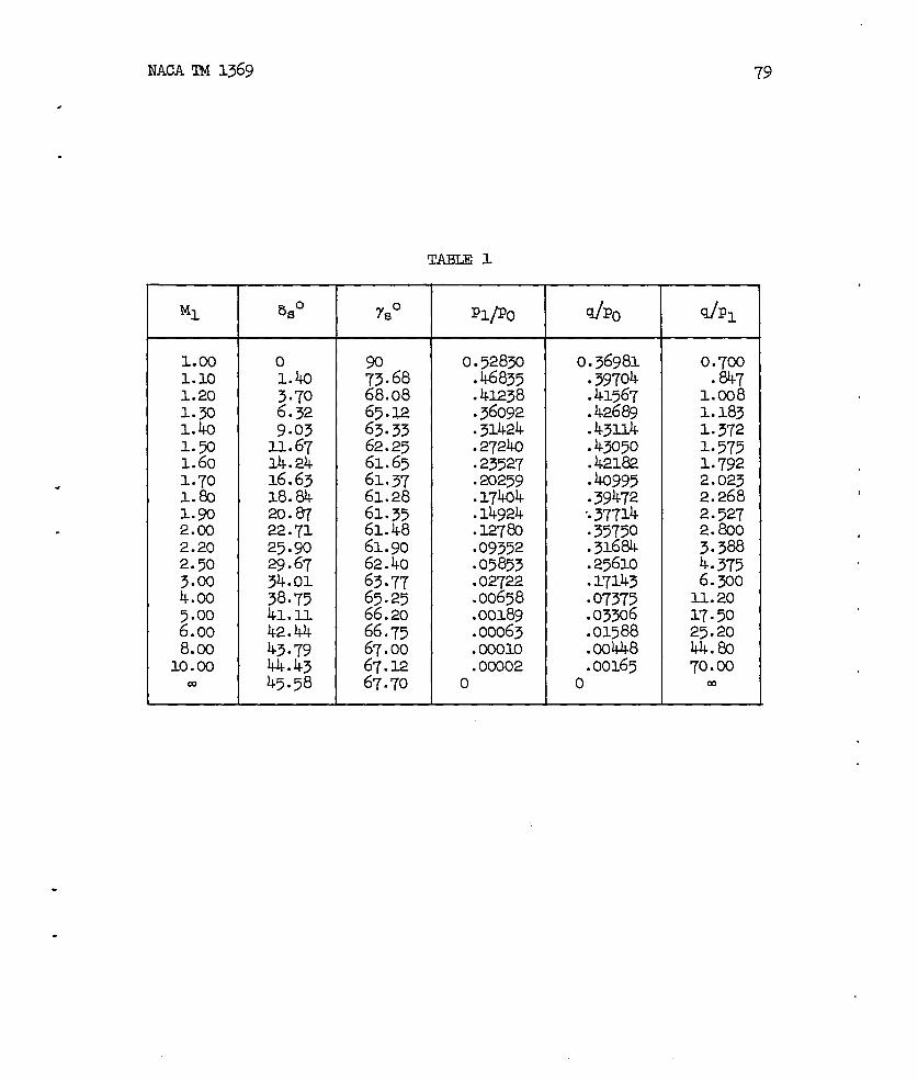
NACA TM 1369
.
.
79
!rABLE1
.
.
Ml 8~o 7s0 P1/P() dPo dP~
1.00 0 0.52830 0s36981 0.7001.10 1.40 :.68 .46835 ● 39704 .e471.20 3.70 68.08 .41238 .41567 1.cQ81.3 6.32 65.12 .36092 .42689 1.1831.40 9.03 63.33 .31424 .431.14 1.3721.X Il.67 62.25 .272ti .43050 1.5751.60 14.24 61.65 .23527 .k2182 1.7921.70 16.63 61.37 .20259
● b995 2.0231.20 18.84 61.28 .17404 .39472 2.2681.90 20.q 61.35 .14924 “.37714 2.5272.00 22.71 61.48 .127&l
● 35750 [email protected] 25.9Q 61.90 .09352 .316% 3.3882.50 29.67 62.40 .05853 .25610 4.375
34.01 63.77 .02722 .17143 6.300::: 38.75 65.25 .00658 .07375 11.20
41.11 66.20 .001892::
.03306 17.5042.44 66.75 .00063 .01588 25.20
8.(x) 43.79 67.00 .00010 .w448 44.W10.CO 44.43 67.I2 .00002 .00165 70.00w 45.58 67.70 0 0 m
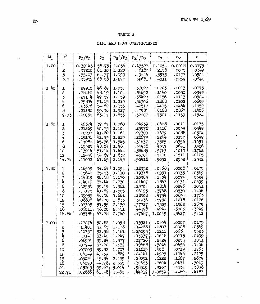
80 NACA TM 1369
TABm 2
LIFT AND DRAG COEFFICIENTS
.
.
Ml p P@?(3 Yo P2‘/P~ P2‘/P() ca c~ E
1.20 1 0.39145 58.75 1.056 0.43527 0.109 0.0018 0:Ol:;2 .37210 61.10 1.120 .k6187 .2158 .0075
.35403 64.37 1.199 .49444 .3373 .0177 .0524?.7 .35952 68.08 1.277 .52681 .4011 .0259 .0641.
1.40 1 .29910 46.87 1.051 .3X27 .0723 .0013 .01752 .284&l 48.19 1.104 .3A692 .1440 .0050 .0349
.27u4 49.57 1.159 .36420 .2156 .0113 ::%;? .27324 51.15 I.219 .38306 .2888 .02026 .23376 54.62 1.353 .42517 .4415 .0464 .10528 .211w 59.36 1.527 ,.47984 .6168 .0%7 .14069.03 .20050 63.17 1.655 .52007 .7321 .1159 .1584
1.60 1 .22374 39.67 I.060 .24939 .0608 .0011 .01752 .2u69 40.73 1.104 .25978 .1116 .0039 .0349
.20207 41.82 I.161 .273CX) .1679 .0088 .0524z .19191 42.93 1.219 .2%79 .2244 .0157 .06996 .172~ 45.36 1.345 .31637 .3385 .0356 ;1008 .15525 48.04 1.484 .34938 .4357 .064110 .13914 51.14 1.644 .3%85 .5783 .1019 .176212 .2.243854.89 1.832 .43101 .7110 .151d. .212514.24 .11022 61.65 2.143 .50418 .9052 .2332 .2532
1.80 1 .16503 %.64 1.054 .18352 .0468 .0008 .01752 .15640 35.53 1.110 .1.9318 .0931 .W33 .03493 .14813 36.48 1.170 .20363 .1404 .0074 .0524
.14019 37.44 1.230 .21407 .M67 .0131 .0699: .12534 39.49 I.362 .23704 .2814 .0296 .10518 .11175 41.69 1.505 .26193 .3768 .Opg .140610 .09935 44.06 1.661 .28908 .4734 .0834 .176312 .08206 46.70 I.835 .31936 .5732 .1218 .2=615 .07303 51.35 2.139 .37227 ;;32; .1962 .267918 .06011 58.oQ 2.551 .44398 .W5 .324918.84 .05788 61.28 2.7ho .47687 1.~45 .3427 .34U2
2.00 1 .w76 30.82 1.058 .13521 .0404 .0007 .01752 .11401 31.65 I.U8 .14288 .oe07 .0028 .03493 .10757 32.58 1.181 1.15093 .1211 .063 .05234 .10141 33.40 1.247 .15937 .1618 .0113 .06996 .08994 35.24 1.377 .17726 .2429 .0255 .10518 .07949 37.22 1.339 .19668 .3246 .0456 .140610 .07005 39.32 1.707 .21815 .408 .0719 .176312 .06149 41.59 L 889 .24141 .4923 .1046 .2E515 .OP24 45.34 2.195 .2&52 .6222 .1667 .267918 .04070 49.78 2.555 .32653 .7604 ..2471 .324921 .03265 55.67 3.014 .38519 .9207 .3534 .383822.71 .02886 61.M3 3.460 .44219 1.0659 .4462 .4187
.
.
.
.
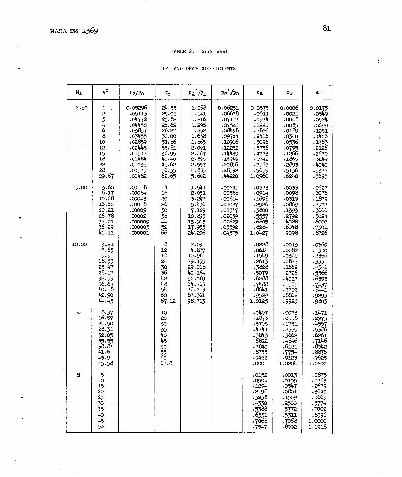
NACA TM 1369 81
.
2.50
p.oo
10.03
m
N
*o
1.2
i6810121518222829.67
2:$10.6816.6020.2126.7851.21,36.29kl.11
3.217.6513.3118.5323.4728.1752.5936.6440.1842.$)044.43
8.3716.5724.x28.3132.0535.5538.8141.643.945.58
510152025
$“
$w
P@o
0.05296.051.13.0kTT2.04450.03857.03455.02859.02~5.01917.01484.01035.03575.00482
.00U8
.0CQ84
.am43
.00318
.0X09
.m2
.Omoog
.000003
.000901
TABLE 2.- Concluded
LIFlANDDRAGCOHC-S
70
24.3525.0525.8226.6228.27y3.0331.8533.8136.9540.4045.6256.3562.65
14162026303844
%
8E1824w364248546067.L2
102030354045w
z67.8
P2’/Pl
1.0681.IklL 2161.2961.k521.6581.%52.0912.4672.8952.5574.8855.602
1.5412.0513.2475.4367.12910.89313.91317.95324.206
2.0914.87710.98119.13529.o1840.16452.oEn64.26376.213W.36198.713
%?’/m
0.06251.06678.071.17.07585.0&98.09704.10916.x232.14439.16949.20816.28592.44220
.w291
.00388
.oi1614
.01027
.01347
.02059
.02629
.OSS92
.04575
%
0.0373.0611.0914.U221.m%.2416.%98.3738.4723.5742.7162.56591.0960
.0523
.0914
.1698
.2926
.3800
.5557
.6Eb5
.&841.0427
.0228
.0614
.1549
.2613
.3&8
.5079
.6288
.7488
.85Q
.95291.0=5
.0497
.1873
.3795
.4741
.5&3
.68U2
.7840
.m35
.gk7E1.0031
.0152
.0594
.1294
.2198
.3238
.4350
.5389
.6331
.7068
.7547
‘%
0.0036.0021.0048.0085.ol@.0340.0536.0795.3.266.1865.2893.5135.6240
.(X)33
.0098
.0319
.0%9
.1393
.2792
.4088
.&)48
.SQ98
.0013
.0082
.0365
.087’7
.1662
.2726
.4017
.5565
.7292
.8862
.9925
.m73
.0558
.1731
.2559
.%62
.4846
.6W
.7754
.91.231.0204
.m13
.o1o5
.0347
.Oml
.1509
.2500
.3772
.531.1
.7068
.8992
0.0175.0349.0524.0699.1051.1406;;76~
.2679
.3249
.4040
.5317
.5695
.0627
.1076
.1879
.2972
.%66
.5024
.6003
.7501
.8726
.O%a
.1340
.2356
.3351
.4*1
.5366
.6393
.7437
.Wl
.9293
.9833
.1471
.2973;455
.6261
.7146
.8042
.8876
.96231.0200
.0875
.1763
.2679
.3640
.4663
.5774
.7002
.83911.oOoo1.1918

82
1.101.2Q1.X~.kol.~o~..601.701.E!Ql.$a2.002.202.503.004.005.006.008.00
10.00m
NACA TM 1369
.
TABLE 3
LIFT AND DRAG COEFFICIENTS OF THE EOUNDARY CURVE
1.43.706.329.03
u. 6714.2416.6318.84m.a22.7125.9029.6734.0138.7541.1142.4443.7944.4345.58
P2po
0.43110s35952.26668.20050.14392.11022.07918.0578a.04047.02886.01417.00482.00073.000014.000001
0000 I
~; ;4
65 763 1062 1561 3961 2261 1761 2161 2961 5462 3963 4665 1566 1266 4567 067 767 41
P2‘/P~
1.1X1.2771.4571.6561.8942.1432.4392.7413.0973.4604.2505.6028.385
15.2524.4035.2563.II98.90
P2 ‘/P()
0.52924.52681.525%.52009.51593.50418.49412.47687.46220.44219.38746.44221.22824.10060.04612.02231.00630.00233
0.2471.4011.6Q35.7321.8339.9052.9697
1.00451.0449I.06651.08831.09601.07351.06501.05151.03621.01711.0121l.oo~
Cw
0.0104.0259.0668.1159.1724.2297.2&7.3427.3983.4465.5284.6242.7243.8551.9107.9432.9692.9895
l.ol@
0.0248.0641.1107.ly34.2068.2532.2988.3412.3812.4187.4855.5695.6747.&25.%52.9136.9601.9&13
1.0200
.
.

NACA TM 1369 83
.
.
1.20
1.40
1.63
1.8)
2.CU
2.50
1o.03
TA2124
um!ANo DRA!3m2FFIclmfm AccoKomG‘m!cE2LJmAPUm TE2J3Rr
*o‘1
233.7
12
9.03
123468
In1214.2k
30121518. W
1012151821=-77.
46
46
12
M2430364244.43
%
o:~3.31a.38357.0jm4.14248.213g2.2W6.42744.569%.64259
.05604- Ixn.16781.22353.335%AA707.55W.67Q$I.m&
.04676
.09325
.lbn
.l%W
.27576
.ml
.4-6626
.555’Z
.69553-m855
.04042
.Oeom
. lzlo2
. tilza
.24182
.yao
. 40X1
.48361-W3.72x%..%643
.om4
.C&Jgl
.o@+5
.12.Ml
.V@9
.0W9
.17037
:%?.42732.47030.5&7ek
.026%a&cEJ
.IA31
.16eJ10
.211249
.25258
.2*7
.3n72
o.0m18.fw%.o1655.@16
.W@
.Co4m
.O1..wl
.olg83
.04483
.Om
. 10I.M
.Ox@
.CU393
.@X79
.01363
[email protected]. 14.oko. lg772
.uw&
. W326
.00734
.o1502
.02932JWz&5
z.1171.18314.28WL
.Wo
.a3281
.03634
.o1125
.02532ok%>.o-/o3a.U51%.15%i9.z2&[email protected]
.-3
.@213
.00479
.W61
.olg15
.05402
.05318.
.07’650
.U62
.17231
.23742
.kti75
.467&9
.00398
.@3@
.03579
.08261
.14321
.w@
.32232
.42Q33
-m.Ca441.01762.03569.o-fo51.11022.lg8m.21.6m
0.01’75.0549
:22
.Oln
.0349
.mkd&l
. U@
.1574
.Olm
.0549
.0524
.0698
:3.1745.20s4.24@
.o175
.039
.oy24
.0698
.1047.
!ij
.ywa
.Olm
.0349
.0524
.0698J047.X@
:%8
.3142-54355-3962
.Oln
.03$9
.qm
.0698
.UA7
.s%
.1745:%8
.0598
.I.Ow
.204
.3142
.4189
.47X2
.57@
.n75
J%98.10k7.*.x42.41e3. 47X?.5760.nm.7735

84
TABLE 5
NACA TM 1369
.
.
Ml @ (caG - cm ) caG (CT/G- %rL) CWG
1.40 1 0.00084 0.07228 02
0.0013.00151 .14399 0 .0050.00163 .21555 .0001 .0113
2 .00385 .28881 .0002 .02026 .01408 .44152 .0010 .04648 .046$10 .61682 .0072 .0%79.03 .08g~ .73209 .0148 .1159
5.00 : .0005 .0523 .0009 .0033.0030 .0914 .0010 .0098
12 .0255 .1698 .0063 .031918 .0696 .2996 .0246 .08!5924 .1391 .3890 .0341 .1393w .1846 .5557 .1433 .279236
● 3972 .6~5 .2698 .408841.11 .466g .8284 .4895 .6048
.

12KNACATM 1369
.
.
85
1=Region
L
12
;
;
789
1011E13141516171819m2122232425
P/Pol
0.31404.3645.2991.3455.2848. 33Q4.2711.3139.3285.3139.2985.2999.2850.2708.3624.3445.3295. 3X24.3276.3134.2972.2996.2842.2696. *1O
TABLE 6
M
1.40041.2931.4351.3321. 46g1.3641.5031.4011.3681.M11.4361.4331.4681.5041.1541.3341.3661.4Q41.3701.4021.4391.4341.4831.507
45.550.644.248.842. g47.141.745.747.045.644.1
&41.7
iii47.045.446. g45.544.044.842.841.6
1.9996
1*9997
1● 9997
1.9998.9997● 9997*9997.9997● 9997● 9997.9982● 9997.9997.9997.9998● 9997.9997.9997● 9997● 9997
.
.

86 NACA TM 1369
TABLE7
(a) Angle of deflection andshocks between the zones
shock angle of the
Regions
;::5.67-88-15
IL- 1613-1714-18M-25
Angle ofi~flection
3.003.032.932.932.932.922.902.932.93
Shock angleP
49.5747.9146.4845.1349.4347.7846. b45.0349.30
Regions
1-32-4
~:;
2:;8-11g-lo
10-1110-1211-1312-13
.
.
(b) Intensity of expansion wavesbetween the zones
IntensityL!@’
1.001.031.00
.891.031.001.001.01
.921.00
.92
.911.02
Regions
13-1415-1616-1716-1917-1817-2018-21”19-2020-2121-2322-2323-24
Intensity2%0
1.021.00
.881.001.06
● 991,00
.891.05
.891.05l.o~
.
.
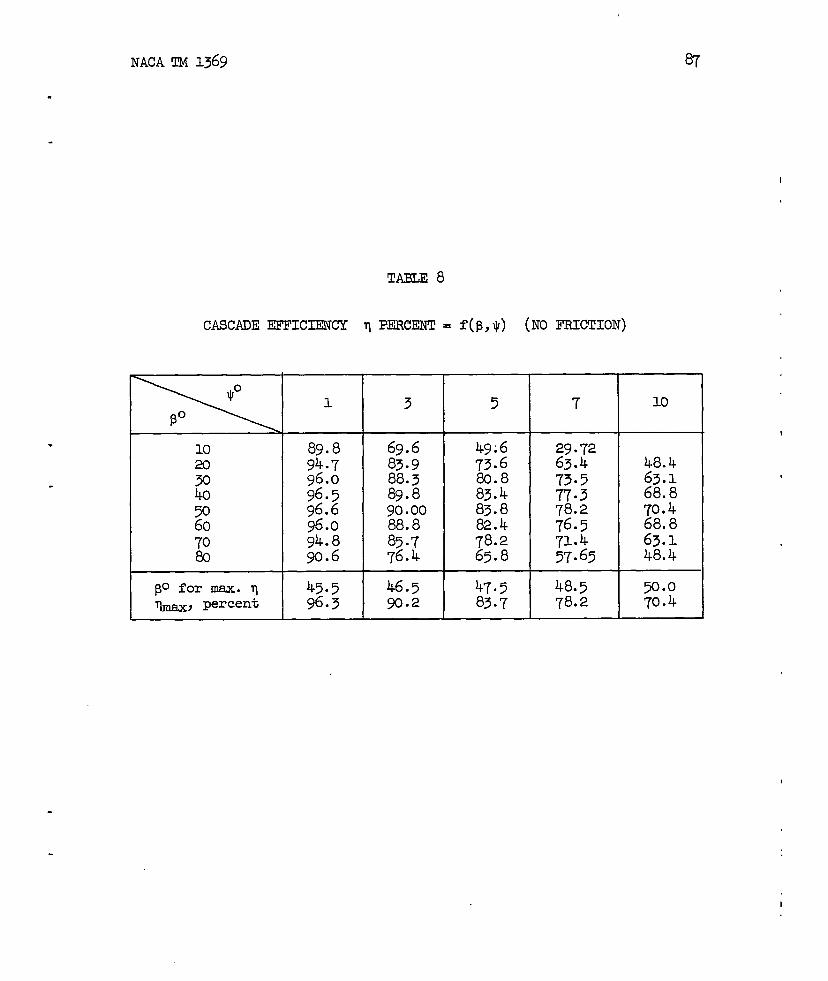
NACATM 1369
.
87
I
!L’ABU8
CASCAOE EFFICIENCY q PERCENT = f(~,~) (NO FRICTION)
.
.
po for max. q 45.5 46.5 47.5~-, percent 96.3 90.2 83.7
I
=-l-=29.7263.473*577”378.276.571.457.65
48.463.168.870.468.863.148.4
I
48.578.2 g::
I
#
I

88 NACA TM 1369
.
.
TABLE 9
CASCADE EFFICIENCY WITH FRICTION ALLOWED FOR
M= 1.40 I M= 2.50
35.8g.;
82;~82.6&).574.757.8
57.0g.:
82:882.7E!O.674.657.2
44.163.971.273*973*569.960.633*5
41.163.771.874.874.771.863.841.4
.
.
.

NACA TM 1369 89
mELE 10
CASCADE EFFICIENCY WITH DOUBLE-WEDGE PROFILE AND FRICTION
M= 1.40 $=3°
.
.
d/Z = 0.05 I d/Z = 0.10
45.5365.2872.5275.1174.8371.5062.7137.18
2$).0447.22;:. ;;
54:8247.3129.25
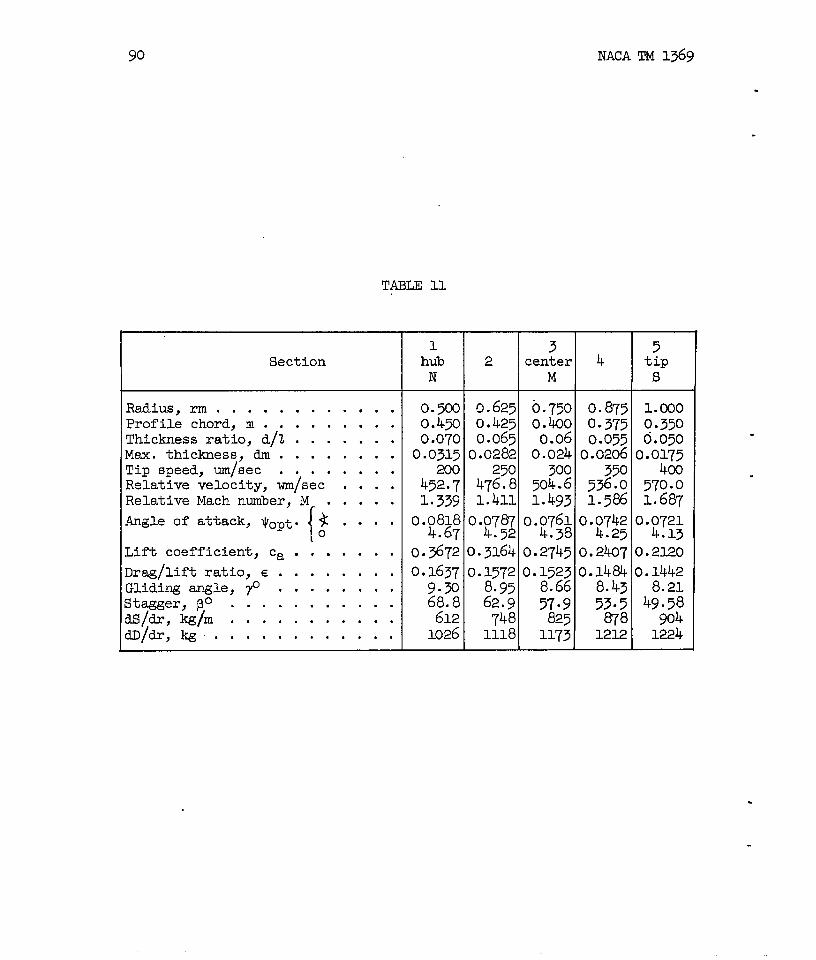
90
TABLE 11
NACA TM 1369
.
Section
Radius, rm . . . . . . . . . . . .Profile chord, m . . . . . . . . .Thickness ratio, d/1 . . . . . . .Mac. thickness, dm . . . . . . . .Tip speed, um/sec . . . . . . . .Relative velocity, wm/sec . . . .Relative Mach number, M . . . . .
[Angle of attack, ~opt. ~ . . . .
Lift coefficient, ca . . . . . . .
Drag/lift ratio, ~ . . . . . . . .Glidingangle, ~ . . . . . . . .Stagger, j3° . . . . . . . . . . .dS/dr,kg/m . . . . . . . . . . .dD/ti,kg. . . . . . . . . . . .
1hubN
o.5m0.4%0.0700.0315
45:1.339
0.08184.67
0.3672
0.16379.3068.86121026
t
32 center
M
0.625 0.7500.425 0.4-000.065 0.060.0282 0.024
250 300476.8 504.61.411 1.493
0.0787 0.07614.52 4.38
0.3164 0.2745
0.1572 0.15238.95 8.666~i: 37*9
8251118 1173
4
0.8750.3750.055
0.0206
532%1.5e6
0.07424.25
0.2407o.14e4
8.4353*5
87812X2
5tips
1.(3000.3500.050
0. O;g
570.01.687
0.07214.13
0.2120
0.14428.21
49g:
1.224
.
.
.
.

NACA TM 1369
.
.
.
91
A// /B2
// ,~
~M,U, -
P2M2 U2
/////A
Figure 1.- Expansion around a corner.
s
u;
u,
B
A////
E%
Figure 2.- Obliquecompression shock.

92 NACA TM 1369
90°
80 1
Ys-70 ~ i
\~
60 ~
50
8~7 I00
40 — ~
30
20 /
to -
0 1234 “56789 10 M
.
.
Figure 3.- Shock and flowdeflectionanglesfor M2 = 1.
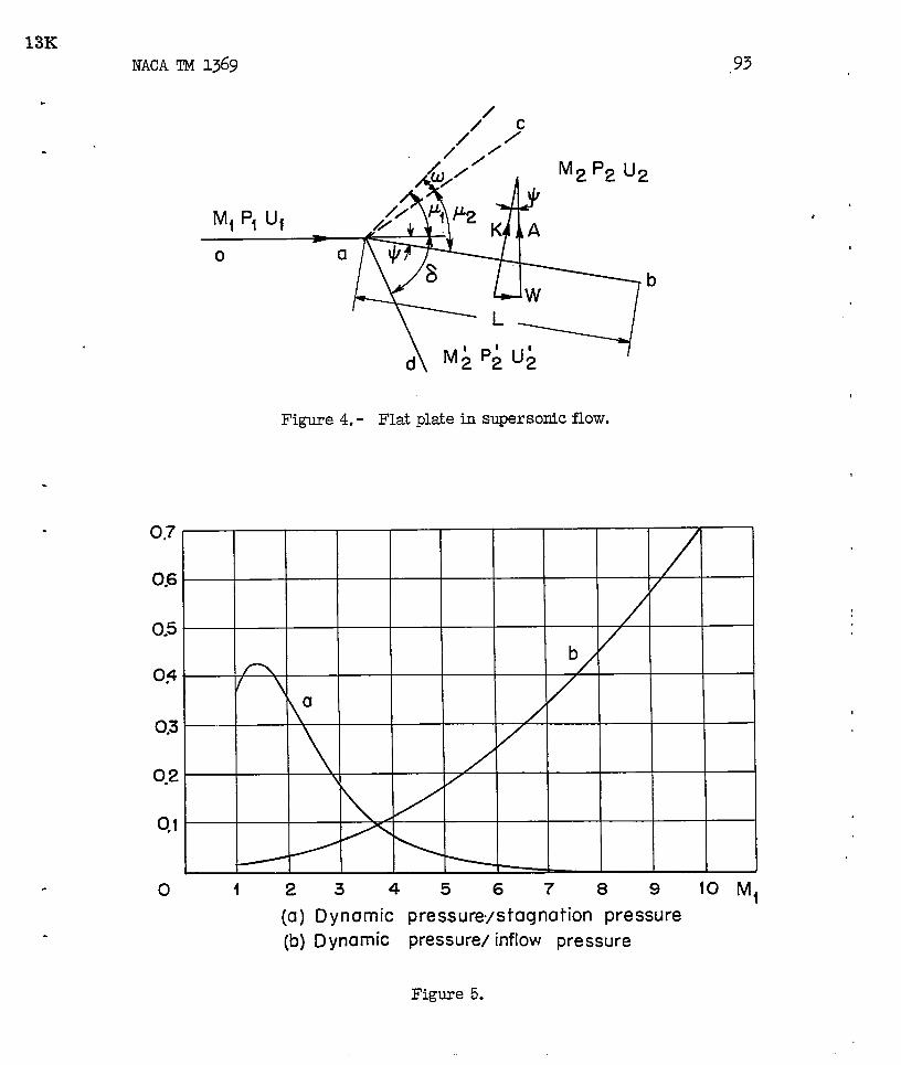
13KNACAm 1369 ,93
.,/ ~
.
Figure 4.- Flatplatein supersonicflow.
0,7
0.6 ‘ /
0.5
b/ ‘
0$/
0.3
0.2 \
0,1
0 1234567 89 10 Ml
(a) Dynornic pressureistaqnation pressure
(b) Dynamic pre.ssurel inflow pressure
Figure 5.

94 NACA TM 1369
1.2
co1.0
0.8
0.2
0
I
M=2
/
Figure 6.- Liftoftheflatplate.
.
.

NACA TM i369
0.6
0.5
Cw
0.4
0.3
0.2
0.!
o 5 10 {5 20 25 30 35 40 45°
+0
Figuxe 7.- Drag offlatplate.
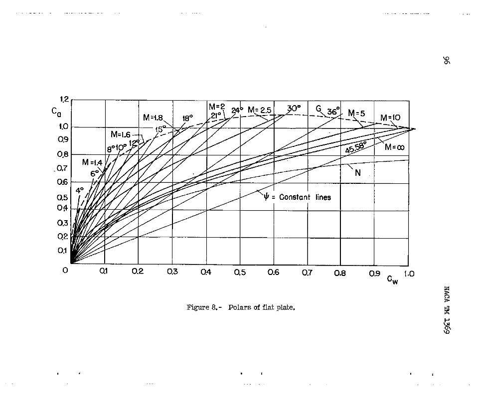
.- .-
KJu-l
1.2
co
1.0
0.9
0.8
.0.7
0.6
0.5
04
0.3
02
0.1
0 OJ 0.2 0,3 G4 ().5 (3.6 0.7 0,8 (39 - [.0
Figure 8.- Polarsofflatplate.
,,
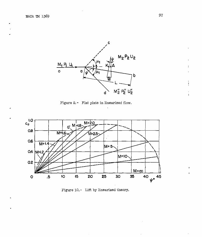
97
.
.
1
1.0C(J
OB
0!6
0.2
0
Figure 9.- Flatplateinlinearizedflow.
.5 10 ~5 20 25 30 35 40 459°
I
,
Figure 10.- Liftby linearizedtheory.
.
.

98
.
O*5
Cw
04
c13
0,2
0.1,
I
M= .4, -,
.Uliiiie
--E+
&M =1.
//
=1.&/
o 5 10 15 20
Figure 11.- Drag by
2>,\\\\\\25 30 35 40
+0 40
.
.
.

. , + , ,
----- Characteristics
— Shock polor
(a) (b) p,> p.\
_-J-=-J-= “:,.\\
(c) (d)S = Blade
(a] Overtaking
(b) Grossing (in free jets)
(c) Reflection
(d] Cascode flow
Figure12.- Interactionbetweenexpansionwaves and compressionshocks.
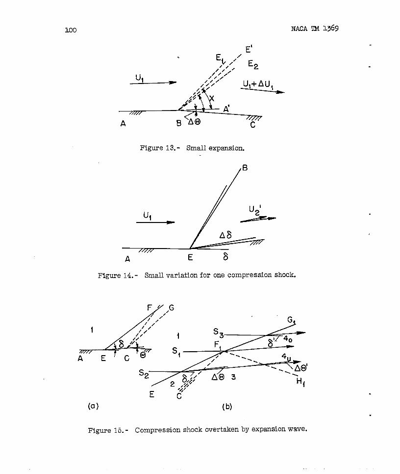
100 NACA TM 1369
Figure 13.- Small expansio~
/
B
u,d
/////
A E 8
Figure 14.- Smallvariationforone compression shock.
1
(o) (b)
Figme 15.- Compression shock overtakenby expansionwave.
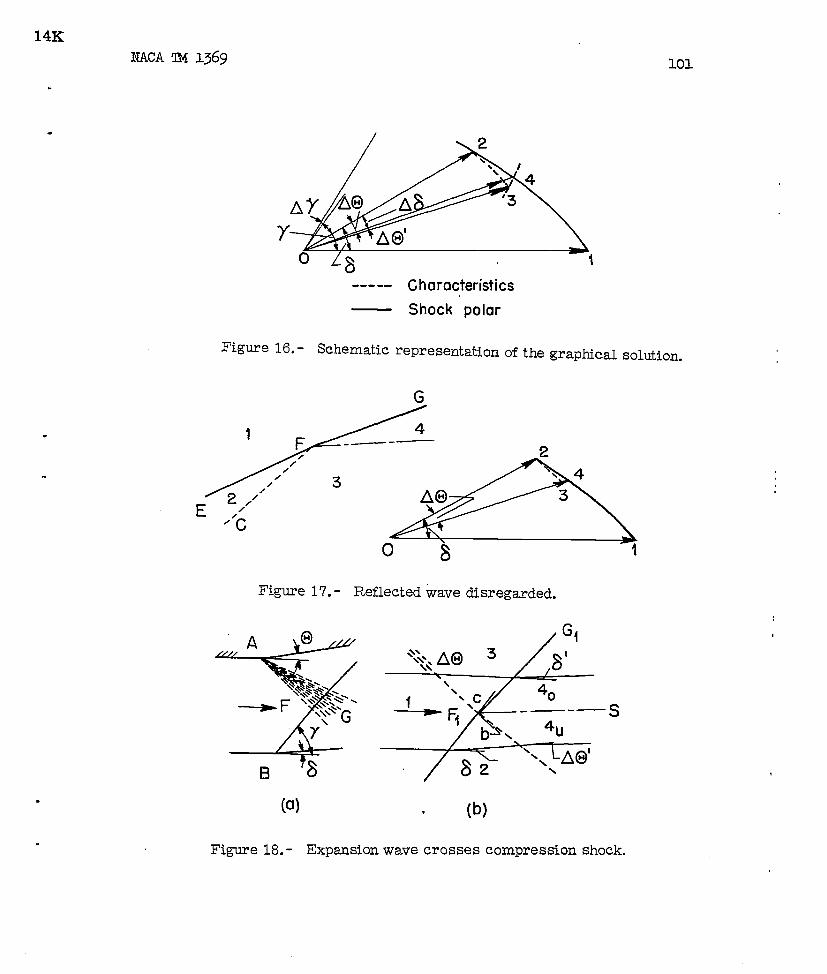
14K
NACA TM 1369
----- Ghoracteriqics
— Shock polar
Figure 16.- Schematic representationof the
101
graphicalsolution.
2
A@
o 8
Figure 17.- Reflectedwave disregarded.
/ lJi
(a) . (b)
Figuxe 18.- Expansionwave crosses compression shock.
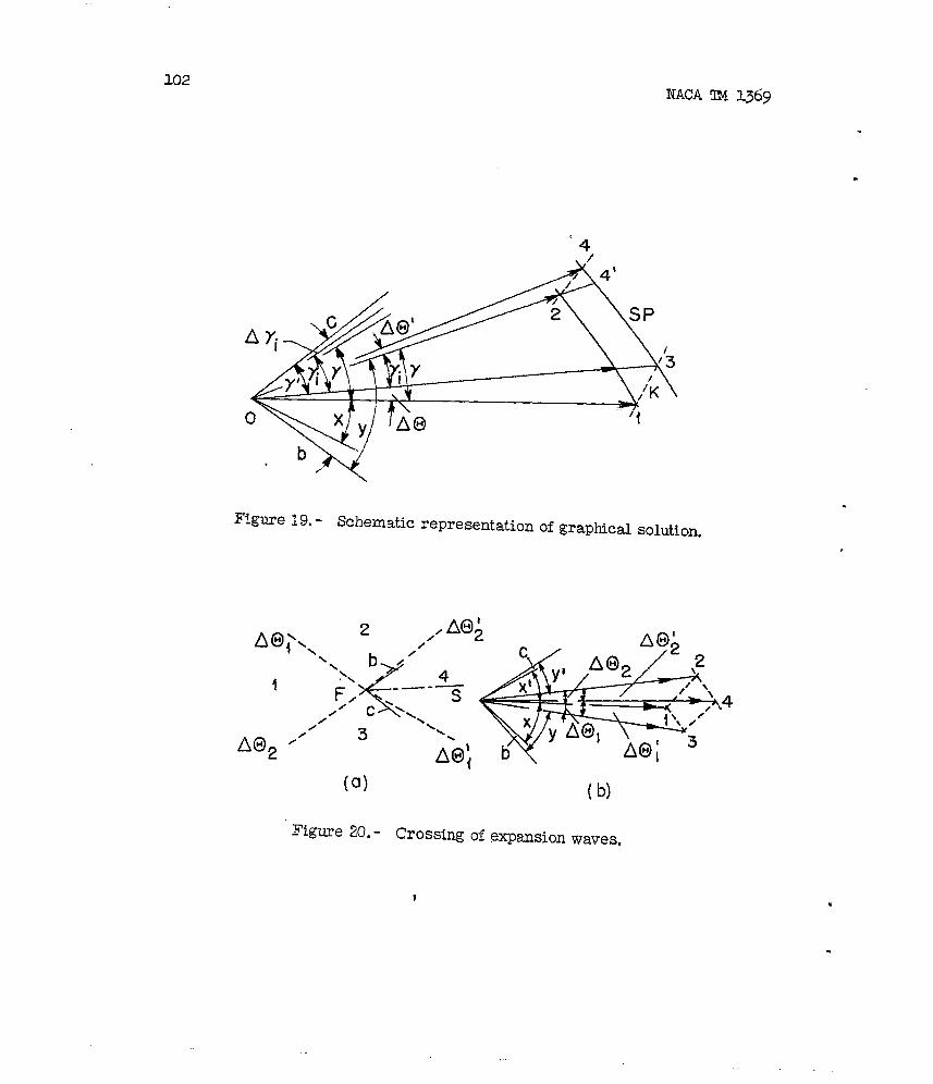
102mm m 13”9
4
.
.
q
o
/
Figure 19.- Schematicrepresentation
‘1
ofgraphicalsolution.
A@2
2 , A@;h \ b /’”\
<
4(; ‘—-— s
c ‘~,///// 3 “~.
(a)(b)
Figure 20.- Crossingofexpansionwaves.
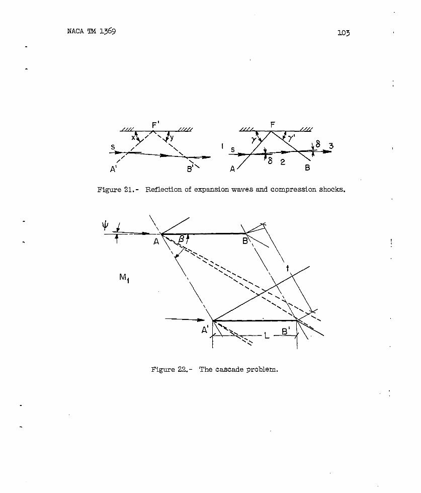
NACA TM 1369 103
.
ad compression shocks.
A’ #\ A/
Figure 21. - Reflectionofexpansionwaves
‘i
Figure 22. - The cascade problem.

-
\
\
1
\A\ 11’g
14
1
Figure23.- Cascade example.
,,
I-Jo-c-
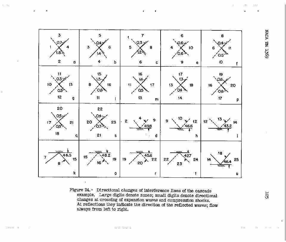
1 ,
3\
A
‘\\o,7
I 4
t. \
2 0
11 ,
<
‘~\o.3 ‘
10 ; i3/
,/’ \
{2 q
2“0
‘\
{
\o.5 ‘
17 ,; 2!
‘Q .,,/
18~
x
746.5
15
8
k
5\\
/
\ ?.43 6
14” \\
4 b
f5
Y
1.5
8 , 16
z~o,/
11
22\
‘,0$ ~
<
20 ;, 23
,Z0,7 .,/
21 s
6 c1 9 e
4z\\v9
~., lo,/y 12
+@% -AK+%
d h
\\.\\\ * -7,~ \\45.6
I ,//
~o>, 22 2:,/’ h, 24/ 23
r t
8
“+.4j4’
6
\
,/ II
//’0.5
10 f
{9
‘\\O.6 ‘
<
t6 ; 20
/’05,~
17 P
12 “.\13>/ ,4
+$%
i
18
x
1446.425
u
Figure 24. - Directionalchangesofinterferencelinesofthecascadeexsmple. Large digitsdenotezones;smalldigitsdenotedirectionalchangesatcrossdngofexpsnstonwaves and compressionshocks.At reflectionstheyhdicatethedtrectionofthereflectedwaves;flowslwaysfrom lefttoright.
,

.
.
P/g0.6
0$
0,2
0
Q2
----
0 0,1 0,2 0.3 0#1 0.5 0.6 0.7 0,8 0.9 1.0
llLPressure at upper side
----- Pressure at lower side
/////// .Resultant pressureResultont pressure by linearized theory
Figure 25. - Pressure variation along the plate (exact method),
Figure 26. - Definition of thrust ad tangential force.
.
.
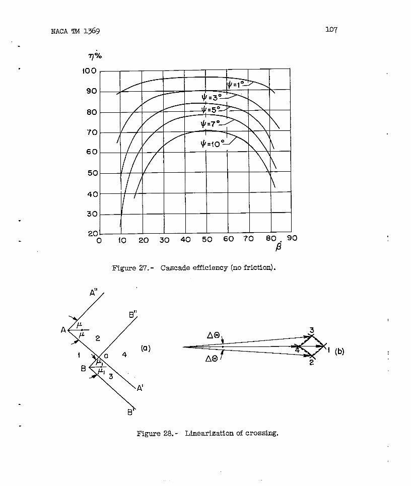
107
.
.
.
.
.
NACA ‘l?M1369
7&
100
90 0
80 4
70 / ‘/
/
60 / /
50 I, f
40 f
30
I20-0 fo 20 30 40
“Figure27. - Cascade
50 60 70 80. 90
P
efficiency (no friction).
d’
1
B
Figure 28. - Linearization of crossing.

108 NACA TM 1369
.
.\rrrz3E5 (d)
K==q “)l+--------- L
.
.
Figure 29.- Linearizedcascadetheory.
.

15K
.
.
NACA TM 1369 109
Figure 30. - Numerical example of linearized cascade theory.
P/Pn
QG‘
09--—-.--
0.2
0 m ~
-0.2-0 0.1 ().2 (3.3 0.4 0.5 (3.6 0.7 0.8 0.9 ~.~
1/P______ pressure on upper side
— Pressure on lower side
////// Resultant pressure
Figure 31. - Pressure distribution over plate by linearized cascadetheory.

110 NACA ~ 1369
.
.
Figure 32. - The profile.
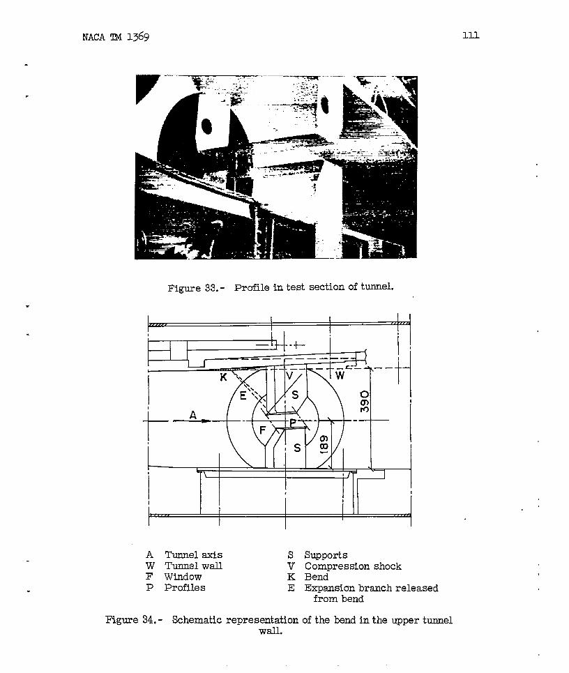
NACA TM 1369 111
Figure 33. - Profile in test section of tunnel.
n.. I II
r“’”I 1 1 r 1 I
I =
A Tunnel axisW Tunnel wallF WindowP Profiles
Figure 34.- Schematic
svKE
representationwall.
supportsCompression shockBendExpansion branch released
from bend
of the bend in the up~r tunnel

112 NACA l!M1369
s
~HK-------------------------------_——____
)-----—---------------------------.------..--.---------.--.----------------+0-_---7*——-
----. ----. -— —----—---
‘~0 Light source S MirrorK Tunnel P Profiles
Figure 35. - Position of optical sxis and shadow formation. x = 8 cm;y= 4.5 cm; Z = 300 cm.
Figure 36. - Profile at starttig.
Figure 37. - Sclitieren diaphragm vertical. Y = OO.
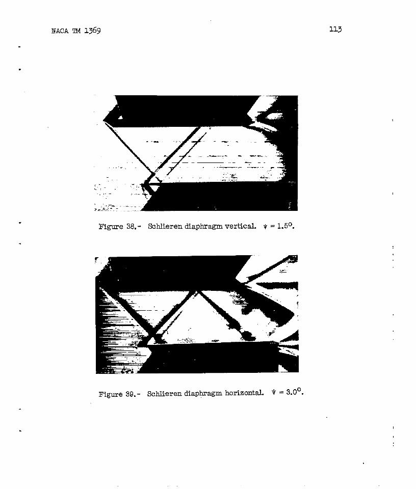
NACA TM 1369 113
.
.
.-.. ,.
-.L’
“.\
~
.-*. ,-. .-.
-.,
..,.. -.. -.--. ,.- - —-.
-.=— -
-. . ---- .._. .7 .-,, ...-
.--L, . . .+~. .---=
Figure 38. - Schlieren diaphragm vertical. V = 1.5°.
Figure 39. - Schlieren diaphragm horizontal. V = 3.0°.
. 1

114 NAC!A~ 1369
Figure40. - Photograph of crossing.
\ \
‘\
Figure 41. - Perspective distortion of figure 23. For comparison withschlieren photograph in figure 39. (O represents the position ofthe light source; the finer lines represent the shadow boundaries ofthe plate and interference line s.)
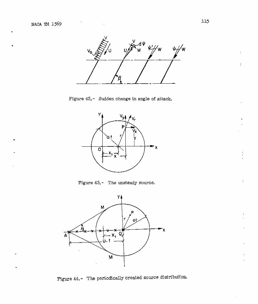
NACATM 1369
.
.
115
.
Figure 42.- Sudden change in angle of attack.
43. - The unsteady source.
Yt
Figure
M
-xA
M
Figme 44.- The periodically created source distribtiiom

116 NACA ’1141369
t
1’
.
.
Figure 45. - The integration limit.
(a)
/
2qpc -2p
Y=c L E / “J
1/ 2PY=0
2 pc
/ ‘
Al c o Dt+x
1-Figure46.-
,,+’-/7t-t
Pressure distribution at y = constant lines.
.
.
.

i6K
.
*
NACA TM 1369 SL7
Yt
Figuxe 47. - Velocity distribution
I
at y = constsnt lines.
%3433+=JBi
‘ (a) (b)
Figure 48. - The flat plate in a gust.
.
.

118
T ~2C” 2PY=0
-&A ,Vo t?t o
- at
F ‘
Ut1
B
(a)
I I
2 Pc
A I I B
(b)
Figure 49, - Pressure
(c)
distribution slong the plate.

119
.
.
.
f
‘o ft+ttt’ :
“0ffttffi ~
o
t+tt+f‘o
Figure 50. - The straight cascade in vertical gust.
B’
Th
B
+h
B{ L
Figure 51. - Start of process. ;
120
I
.
.
‘o
1’
A’
A
Figure 52. - t > h/a
r
B’
B
B “
B’
I
r IllltI
B
‘o 444 N/?+ v+tv!+t+t+f+tl ~ h I/
A“ 1 ~ B“/I ‘--- - o’~
.I+=-=L-’
.
.
●
Figure 53. - Second phase of additional pressure.
, ,6
IillE=l‘o F
B
ot=o
‘B,h?= co)
F
A
ID
B
tl; .(3,251
A b’ (7’4)F
$
,A(OB v;.OS
2,
d’ ~, (q=2)
IF
@
A:.B tg=o,754
3,
A’‘B, (q.t#327)
F
@
A; ~B”tl~n
4,’
A’ ‘@ (7:1)’
\
=!.!77
5=0,B5)
q4.4t46
(q=omr)
I +F
\\
4.sA!qif-F./
..,,
tl+ ,333 0
‘,A’ B = Om
\ ‘\
w
F
/11
A
V; ,4~ o9,
A’B’ (7=0,244)
I ‘\
\\
Figure 54. - Locationofgustfrontsnddisturbedareasatvsztoustime intervals.
. ,
122 NACA TM 1369
p/~ W0.90.60.70.60.s0.4
0.30.2O.to/ A
.
.
Figure 55. - Pressure of undisturbed plate pu.
Pn /p g-t
0:8-oo7-0.6-
0.5- “o.4-
6::-
Ao.1-
B
I
A’0s ‘B’ bG o~
Figure 56, - Pressure contributionph.
NACA TM 13691.23
.
.
.
‘Jy/~o to-0.8.
Q6 .
0.4.
0.2-
A o-
A I
*
:
Figure 57. - Velocity distributions vy/vO at times 5, 6, 7, and 8.
‘1=0.85
I
II
III --1 :1I II I
, I ,
0.2 -0.1 0 +Q.j 0,2
I
~ “:5
III q= 0.707 4
II ~=-o.4I 3II
I
I I1
2
I I
*+E + ‘-- 1I
I I
-c, 0,5 Oi & 02 0.10
~,
I1-
:I
I II
I
1
I
f6 7 =0.5
4 ~= 0.55
3
-2
.1
77=0.30
IIIII
{A,fII
I
f
I{.098
76
54
32
4I I
) 0.950.9 0.8 0.7 0.6 0.3 0.4 OB
Figure 58. - Functions f forvarioustime intervals.

124NACA TM 1369
. Figure 59.
0.7-0.6-
0.3- 6
I
dI
o~05 B’06
Figure 60. - Pressure contribution pv.
Pt/pc
t.o
0,8
0.6
0.4
1
O.z
o
0.2-1
0.4
0.6 4
0.8
i1
.
.
A B
Figure 61. - Resultant presswe distributions.

17K125
.
A/A’ 1‘
08
0.6
0.2
1,0 i 2 3 4 t/
M
Figure 62. - Lift of plate.
‘h-5
/M~t, 1
0.8
0.6
09
Q2
o 1 2 3
distribution M referred to plate center.I
.
.

126 NACA TM 1369
T ‘/0
90
80
70
60
50
40
30
0
Figure 64. - Allowance for friction,
Ia
//
r
#11
\
10 20 30 40 50 60b“ 80
(a) No frictio~(b) With frictiom M = 1.40, (c) With fr&.i:&
(b’) With::i~3~~o M = 1.40, (c’) With frictio~?= . . $ = 4.110.
M = 2.50,
M = 2.50,
.
.
Figure 65. - Cascade efficiency. “

12-(
w“
T“
-—
Figure 66. - Allowance of fhite thickness ratio.
90
a80
70
b
60 \3
50c
40
30 ,
20- ,
10 20 30 40 50 60 P“ 80
(a) d/t =0 (b) dtt =0.05 (C)diz =0.40 M=l.4~,*=30
I
Figure 67. - Efficiency of cascade of double-wedge profiles.

128 NACA TM 1369
.
.
A
u/ ‘“r
\
B
- u
A’ P’ 0’ I
.
Figure 68. - Area disturbed by leading edge of a blade assumed asflat plate.
.
.

18KNACA TM 1369
.
.
rm
1.00
0.75
0.50 , I
O 2 4 6“/0
Cl/l
Figure 69. - Blade chord, maximum thiclmess, stagger, and lpcationof cross sections.

130 NACA TM 1369
.
.-7II\II1IIIIIII1IiIII1I1I
.
.
\!
-Y-1
Figure 70, - Blade form, blade form without angular rotation,
1.25“ ~
1,0 b
0.75
0.5.
.
0.5 075 {m
(N) (M) (s)
(a) d Sidr X10-3 kg/m. (b) dD\drx10-3 kg...
Figure 71.NACA . Langley Field, Va.


![INDEX [maheshkhati.com] · CHAPTER1 INTRODUCTION Power ... of blades and generating thousand kilowatts of power. But, ... In this case motion of the blade and wind has same direction](https://img.pdfslide.us/doc/110x75/5af334347f8b9ac24691a932/index-introduction-power-of-blades-and-generating-thousand-kilowatts-of.jpg)