arX

iv:c

ond-

mat

/980

3051

v1 [

cond

-mat

.sta

t-m

ech]

4 M

ar 1

998

UNC-CH-MATH-98/1

Folding the Square-Diagonal Lattice

P. Di Francesco*,

Department of Mathematics,

University of North Carolina at Chapel Hill,

CHAPEL HILL, N.C. 27599-3250, U.S.A.

We study the problem of ”phantom” folding of the two-dimensional square lattice, in which

the edges and diagonals of each face can be folded. The non-vanishing thermodynamic

folding entropy per face s ≃ .2299(1) is estimated both analytically and numerically, by

successively mapping the model onto a dense loop model, a spin model and a new 28

Vertex, 4-color model. Higher dimensional generalizations are investigated, as well as

other foldable lattices.

02/98 PACS: 64.60.-i Keywords: membrane, folding, entropy, vertex model

* e-mail: philippe@math.unc.edu

1. Introduction

Models for polymerized membranes can help our understanding of biological systems.

A typical discretized model for a membrane consists of a network of vertices (atoms) linked

by bonds. Irregular networks correspond to fluid membranes, with arbitrary connectivity

at each vertex. Regular networks are called tethered membranes: their bonds may have

short variations in length, leading to a geometrical crumpling transition [1]. Continuous

versions of these models have confirmed this result, both analytically [2]-[4] and numerically

[5]. In the present paper, we consider a discrete model for rigid bond-membranes, repre-

sented by regular 2-dimensional networks whose vertices are linked through rigid bonds

of fixed length. The only possibility for such a membrane to modidy its spatial configu-

ration is through folding along its bonds, serving as hedges between adjacent faces. The

effects of self-avoidance on discrete folding models can be extremely complex: already in

one dimension, this has lead to interesting developments, in relation with the ”meander”

problem [6]. The type of folding we consider however is not self-avoiding, in the sense that

we allow the membrane to interpenetrate itself (phantom folding).

This work follows a previous study of the folding of the triangular lattice [7], leading to

an exact result for the folding entropy in two dimensions [8], and to evidence for a first order

folding transition between a flat and a folded phase [9], and some further developments in

which the triangular lattice is folded into the 3-dimensional Face Centered Cubic lattice

[10].

In this paper, we consider the folding problem of the square-diagonal lattice (see

Fig.1 below), made of the square lattice with bonds joining all first and half of second-

neighbor vertices. In a first step, we study the two-dimensional folding of the lattice and

obtain estimates for its folding entropy. In a second step, we introduce d-dimensional

generalizations in which the lattice is folded onto a regular d-dimensional lattice, allowing

only for a finite number of possible relative foldings of adjacent faces of the membrane in

the target d-dimensional space. Estimates for the higher-dimensional folding entropies are

also found.

The paper is organized as follows. In Sect.2, we introduce the 2-dimensional folding

problem of the square-diagonal lattice as an edge tangent-vector model. A reformulation as

a colored loop model leads to some analytic bounds on the folding entropy. The structure

of the colored loop model is further investigated in Sect.3, in relation with the Temperley-

Lieb algebra and the Potts and 6 Vertex models. This leads to better analytic bounds

1

on the entropy. In Sect.4, we transform the colored loop model into a 28 Vertex model,

allowing for the numerical study of the folding entropy, carried out in Sect.5.

The next two sections are devoted to higher dimensional generalizations of the square-

diagonal lattice folding. The idea is to fold the lattice into a target d-dimensional lattice.

We find two such lattices compatible with the square-diagonal lattice: the Hypercubic-

Diagonal (HCD) and Face-Centered Hypercubic (FCH) lattices. The HCDmodel is studied

in Sect.6, and successively mapped onto a colored loop model and a vertex model. Various

estimates of the folding entropy follow. In Sect.7, an analogous study is carried out for the

FCH model. The equivalent vertex model is particularly simple and gives access to very

good numerical estimates of the folding entropy.

In Sect.8, we present a classification of all possible compactly foldable lattices in two

dimensions. In addition to the known square and triangular lattices, we find only two

more: the square-diagonal lattice studied in this paper, and the double-triangular lattice,

a decoration of the triangular lattice obtained by adding vertices in the middle of one

third of its edges (one per triangle), and by drawing the corresponding heights. The latter

lattice is then folded in both 2 and higher dimensions, giving rise to new vertex models on

the Kagome lattice.

We gather a few concluding remarks in Sect.9.

2. The Folding Problem

2.1. Folding of the Square-Diagonal lattice

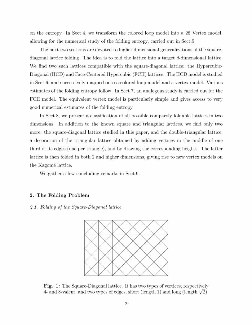
Fig. 1: The Square-Diagonal lattice. It has two types of vertices, respectively4- and 8-valent, and two types of edges, short (length 1) and long (length

√2).

2

We consider the Square-Diagonal lattice, obtained from the standard square lattice by

drawing the two diagonals on each face (see Fig.1). This introduces two types of vertices,

with respectively 4 and 8 incident edges, and two types of edges, short with length 1 and

long with length√2. All the faces of the lattice are triangular, with one 4-vertex and two

8-vertices, and one long and two short edges forming a right angle.

The similarity of all the faces makes it possible to define a complete folding of the

lattice, in which the edges serve as hinges between adjacent triangles, and might be either

completely folded or not folded at all. A folding configuration of the lattice is therefore a

continuous map ρ from the lattice to itself, which preserves its faces, namely the distances

between the vertices around each triangular face. Note that a folding configuration does not

distinguish between the various physical realizations of the actual folding of the lattice,

nor is such a configuration granted to be realizable physically. This is called phantom

folding, where the lattice is allowed to interpenetrate itself for the foldings to be realized,

as opposed to the more realistic, but much more constrained self-avoiding folding.

e2 e1

Fig. 2: The edge vectors for the square-diagonal lattice. In the basis (~e1, ~e2),the short edge vectors are of the form (±1, 0), (0,±1), and the long edgevectors are of the form (±1,±1).

To describe the folding configurations of our lattice, we note that such a configuration

is entirely determined by the list of all the images of the edges of the initial lattice. Let us

characterize these edges by the associated tangent vectors ~t, subject to the face rule

∑

~t around

a face

~t = ~0 (2.1)

There are basically two choices of orientation of all the edge vectors, we fix one as in Fig.2.

Fixing an orthogonal basis of the plane with two short vectors, denoted ~e1, ~e2, we see that

the short edge vectors may only take the 4 values ±~e1 and ±~e2, whereas the long edge

vectors may only take either of the 4 values ±~e1 ± ~e2.

3

A folding configuration is characterized by the images of these tangent edge vectors

(note that short vectors are mapped to short vectors, and long vectors to long vectors).

The requirement that the faces be preserved amounts to the condition that the face rule

(2.1) be preserved by the map ρ. In other words,

∑

~t arounda face

ρ(~t) = ~0 (2.2)

This condition has to be satisfied by the images of the edge vectors around all the faces of

the lattice.

With these conditions, the partition function ZSD of the folding problem of the square-

diagonal lattice (actually of a portion thereof, made of N triangular faces) is simply the

number of distinct folding configurations, namely of distinct configurations of edge vectors

satisfying the conditions (2.2). The thermodynamic entropy per triangle sSD is then

defined as the limit

sSD = limN→∞

1

NLogZSD (2.3)

(a) (b)

- e1 e2

e12- e

2- ee1

e2 - e1

- e1

2- e

2- ee1

e2 - e1

e1 e2

e12e

1ee2

e1 e2

e2 1ee2

e1 e2

e1

2e

e2

e1

e1

Fig. 3: The short edge-vector images for the flat (a) and completely folded(b) configurations of the square-diagonal lattice. In case (b), the whole latticeis folded onto the shaded triangle.

With these definitions, we may already distinguish two particular folding configura-

tions: the flat configuration corresponds to no folded edge, hence has the edge vectors of

Fig.3(a). The completely folded configuration corresponds to folding the whole lattice onto

one single of its triangular faces. The map therefore sends all the long edges onto one of

them, say −(~e1 + ~e2) for definiteness, and half of the short edges to ~e1, the other half to

~e2, as shown on Fig.3(b).

4

2.2. Loop Gas Reformulation

Let us consider a folding configuration of the square-diagonal lattice. The images of

the short edge vectors characterize the configuration completely, as the long edge vectors

may be deduced from the face rules (2.1). But these are still constrained as follows.

(i) the two short edge vectors around each face must be perpendicular, i.e., one of them

is equal to ±~e1 and the other to ±~e2.

(ii) any two adjacent triangular faces sharing a long edge have short edges with either of

the two possible images below

u

v

u v--

v

u

(2.4)

corresponding respectively to an unfolded or folded long edge.

The two conditions (i)-(ii) above are the only constraints on the images of the short

edge vectors. The image of a given short edge vector ~t reads

ρ(~t) = ǫ~ei (2.5)

and is characterized by the pair (i, ǫ), where i ∈ {1, 2} can be thought of as a color of the

edge, and ǫ = ±1 is a sign. In the condition (ii), the signs are the same for the short edges

of the same color. Hence these signs are preserved along chains of short edges throughout

the lattice, forming loops of either color 1 or 2.

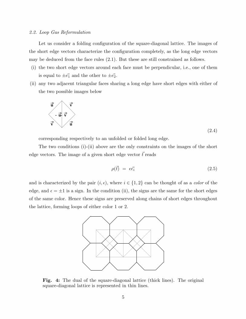
Fig. 4: The dual of the square-diagonal lattice (thick lines). The originalsquare-diagonal lattice is represented in thin lines.

5

More precisely, let us consider the dual of the square-diagonal lattice, whose vertices

are the centers of the triangular faces, and whose edges cross the former ones. This dual

has only square and octagonal faces as depicted in Fig.4. The short edges are in bijective

correspondence with the edges of the square faces in the dual lattice, hence we paint them

with the corresponding colors i = 1, 2, which we will call black (solid lines in the pictorial

representations) and white (dashed lines in the pictorial representations).

e1

e1e2

e2e2e1

η

ηη

ε

ε

e1σ σ

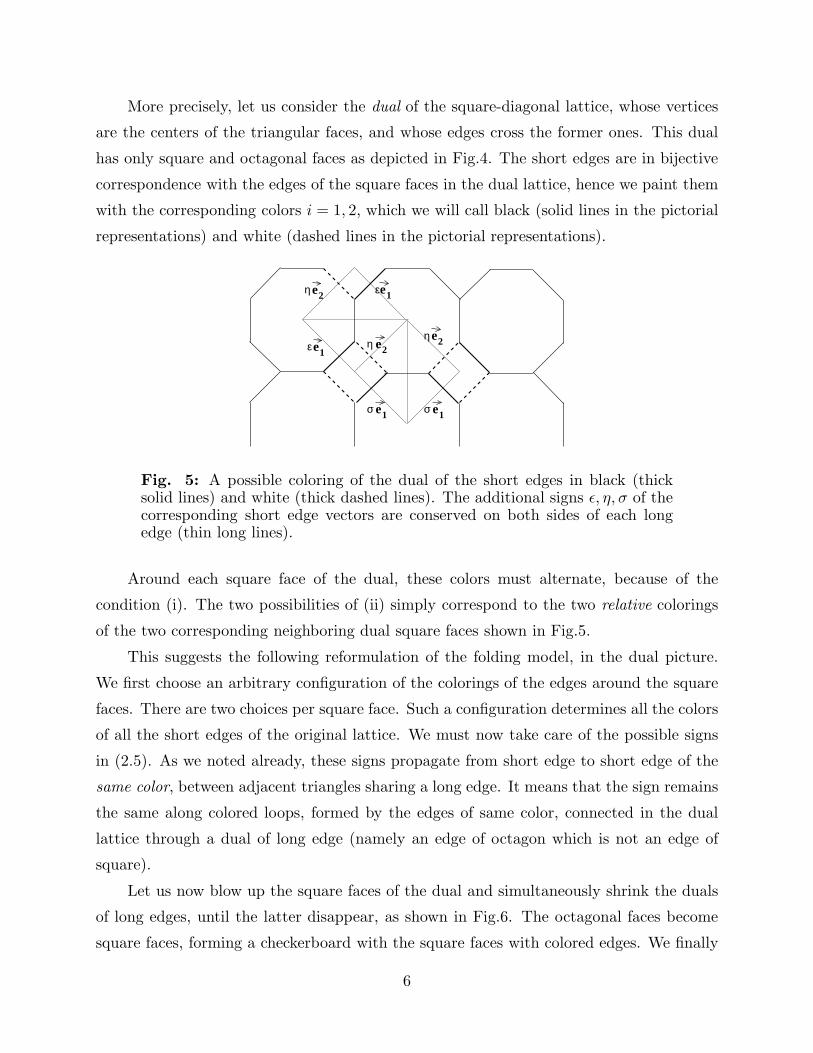
Fig. 5: A possible coloring of the dual of the short edges in black (thicksolid lines) and white (thick dashed lines). The additional signs ǫ, η, σ of thecorresponding short edge vectors are conserved on both sides of each longedge (thin long lines).

Around each square face of the dual, these colors must alternate, because of the

condition (i). The two possibilities of (ii) simply correspond to the two relative colorings

of the two corresponding neighboring dual square faces shown in Fig.5.

This suggests the following reformulation of the folding model, in the dual picture.

We first choose an arbitrary configuration of the colorings of the edges around the square

faces. There are two choices per square face. Such a configuration determines all the colors

of all the short edges of the original lattice. We must now take care of the possible signs

in (2.5). As we noted already, these signs propagate from short edge to short edge of the

same color, between adjacent triangles sharing a long edge. It means that the sign remains

the same along colored loops, formed by the edges of same color, connected in the dual

lattice through a dual of long edge (namely an edge of octagon which is not an edge of

square).

Let us now blow up the square faces of the dual and simultaneously shrink the duals

of long edges, until the latter disappear, as shown in Fig.6. The octagonal faces become

square faces, forming a checkerboard with the square faces with colored edges. We finally

6

(a) (b)

Fig. 6: We start from an arbitrary bicoloring of the dual of the short edges,in the dual lattice (a). We next blow up the square faces of the dual latticeand shrink the remaining octagon edges to zero, so as to get a (bicolored)square lattice (b). We have represented on (b) a new square lattice S in thinsolid lines; each of its faces contains one bicolored square.

draw the square lattice (denoted by S) with vertices at the center of these new square faces

(see Fig.6). The faces of this square lattice simply read either

or

(2.6)

according to the previous coloring. Note that the black (resp. white) edges are connected

between adjacent faces, thus forming lines across the lattice. Discarding the problem of

boundary conditions, we may assume that the lattice geometry is toroidal (namely we

consider a rectangle of size P ×M of lattice, for a total of N = 4PM triangular faces, with

doubly periodic boundary conditions) and thus these lines form loops. The sign of (2.5)

takes the same value along each such black or white loop. Denoting by Nb (resp. Nw) the

numbers of black (resp. white) loops formed by the coloring configuration, the partition

function of the folding problem of the square-diagonal lattice reads

ZSD =∑

coverings of S

with or

2Nw+Nb

(2.7)

where the coverings of the faces of S correspond to the various coloring configurations, and

the factor 2 per black or white loop simply counts the possible choices of signs in (2.5).

We have therefore reformulated the folding problem as a dense loop gas problem,

with a fugacity 2 per loop, and the presence of both loops (black) and their orthogonal

trajectories (white).

7

2.3. Bounds and Expansions of the Folding Entropy

As an immediate consequence of (2.7), let us show that the square-diagonal lattice

folding problem has a non-vanishing thermodynamic entropy sSD (2.3). Indeed, we have

the minoration

ZSD ≥ 2N/4 (2.8)

obtained by counting the coloring configurations of the faces of S, i.e. a factor 2 per square.

The factor N/4 follows from the fact that each square corresponds to 4 triangles in the

original lattice. We therefore find

sSD ≥ 1

4Log 2 = .1732... (2.9)

and the thermodynamic entropy does not vanish.

Another way would have consisted in choosing a particular coloring configuration of

the faces of S, maximizing the number of black and white loops. This is readily obtained by

letting the face configurations alternate between the two possibilities of (2.6) thus forming

a checkerboard. Note that there are two such ”groundstates”, obtained from one another

by exchanging the two face configurations. Restricting to one of these two colorings of S,

we get the following minoration

ZSD ≥ 2Nb+Nw = 2N/4 (2.10)

where we have counted one (black or white) loop surrounding each vertex of S, hence a

total number N/4. This again leads to (2.9).

Fig. 7: A local excitation of a groundstate for ZSD. It is obtained by flippinga face of S, while the rest of the groundstate configuration remains fixed. Thiscreates 2 larger loops of black and white colors, by suppressing two minimalloops, one white and one black.

8

The advantage of this latter approach is to allow for a perturbative expansion of ZSD,

starting from one of the above groundstates, in terms of elementary local excitations.

Such an excitation is simply the reversal of the coloring configuration of one face of S, as

displayed in Fig.7. Doing this will affect the 4 loops (2 white, 2 black) surrounding the

face, resulting in two larger loops, one black and one white. Overall this suppresses two

loops, hence contributes an extra factor 1/4 to the partition function. There are N/4 of

these excitations, hence

ZSD = 2N/4(1 +1

4

N

4+ ...) (2.11)

Fig. 8: The four elementary excitations forming a 2×2 square. These replace4 black and 5 white loops by 1 white and 2 black ones, resulting in a relativeweight 1/26 instead of the expected 1/28 for four distant local excitations.The role of black and white loops is exchanged when the four excitations areshifted by one face.

This expansion can be continued for higher numbers of excitations, but these might

interact, by creating or suppressing more loops when they are close together than when

they are separated. The first instance of this occurs for 4 excitations. Generically, 4

excitations will contribute an extra factor of 1/28 to the partition function, except when

these form a 2× 2 square, as illustrated in Fig.8. Indeed, in that case, a loop is created in

the center of this square, and the factor is increased to 4/28 = 1/26. This is interpreted

as a contact interaction energy between the excitations. This phenomenon propagates to

higher orders. For instance, this is further increased when 6 excitations form a 2 × 3 or

3× 2 rectangle, resulting in a factor 1/28 instead of the expected 1/212 if excitations did

not interact. Up to 6 excitations, the contributions to ZSD read (for convenience, we set

9

N/4 = n)

ZSD = 2n(

1 +n

22+

(

n

2

)

1

24+

(

n

3

)

1

26+

[

(

n

4

)

1

28+ n(

1

26− 1

28)]

+[

(

n

5

)

1

210+ n(n− 4)(

1

28− 1

210)]

+[

(

n

6

)

1

212+ n

(n− 4)(n− 5)

2(1

210− 1

212) + 2n(

1

28− 2

210)]

+ ...

)

(2.12)

The first line of (2.12) includes terms up to four excitations. The bracket includes the

replacement of the expected 1/28 term by the actual 1/26 explained above. This occurs

with a degeneracy n, corresponding to the freedom of moving the center of the 2 × 2

excitation on the lattice. The second line in (2.12) corresponds to 5 excitations. Again, we

have replaced the expected 1/210 by 1/28 whenever a 2× 2 excitation is formed, together

with another single excitation. Those arise with a multiplicity n(n− 4). Finally, the third

line of (2.12) corresponds to 6 excitations. We have first replaced the expected 1/212 by

1/210 whenever a 2×2 excitation is formed, together with two other single excitations. This

occurs with the multiplicity n× (n− 4)((n− 5)/2, for the choice of the center of the 2× 2

excitation among n vertices, and the pair of remaining excitations among the remaining

(n−4) faces. But doing so we have neglected the occurrence of 2×3 and 3×2 rectangular

excitations, for which the previous 1/210 must be replaced by 1/28. This occurs 2n times

(n per rectangular shape), but we have to subtract all the terms in which these rectangles

have been counted as a 2 × 2 square plus two excitations, namely 4n terms with weight

1/210. We deduce the following Mayer expansion of the thermodynamic entropy

sSD =1

4Log(2(1 +

1

4+

3

44− 9

45+

18

46+

1

44+ ...)) = ≃ .231... (2.13)

(i.e. a partition function per triangle of zSD ≃ 1.259...) including the effects of up to

6 local excitations. Note that there are negative and positive terms in the expansion

(2.13), so it is not clear whether this estimate lies above or below the exact value of sSD.

It is possible however to prove that the first two terms give a strict lower bound on the

entropy. This indeed amounts to neglecting the interactions between the excitations, hence

to underestimate Z (as we under-count the loops). We therefore get a first lower bound

sSD >1

4Log(

5

2) = .22907... (2.14)

corresponding to a partition function per triangle of 1.2574...

10

3. Loops and the Temperley-Lieb Algebra

3.1. The Dense Loop Gas

The formulation of the square-diagonal folding problem as a coloring problem has left

us with a gas of dense black and white loops, each weighed by a factor of 2.

Here, we recall some known facts about the dense loop gas on the square lattice S.

The idea is to generate a dense set of black loops on S, in the same way as we did for

black and white loops, except that all the dashed lines are erased. Each loop is weighed

by a factor β, resulting in a partition function

Zβ =∑

coverings of S

with or

βL

(3.1)

where L denotes the number of loops formed by the black lines.

The model is intimately related to both Q states Potts and 6 Vertex models at infinite

temperature, in that it has a straightforward definition in terms of the Temperley-Lieb

algebra [11]. Indeed, let us introduce the abstract ”face” operator

ei = . . . . . .

= 1⊗ 1⊗ · · · ⊗ 1⊗ e⊗ 1⊗ · · · ⊗ 1

(3.2)

acting on a row of 2P parallel black lines. In (3.2), the face operator e acts on the i-th and

(i+ 1)-th lines, by connecting them. The definition (3.2) makes transparent the following

algebraic relations satisfied by the ei’s

e2i = β ei

eiei±1ei = ei

eiej = ejei for |i− j| > 1

(3.3)

easily checked pictorially. The algebra generated by the abstract generators 1, e1, e2, ..., e2P−1,

subject to (3.3), is called the Temperley-Lieb algebra, denoted by TL2P (β).

= β =

Fig. 9: The first and second relation of (3.3).

11

The first relation in (3.3) is consistent with the weight β per loop in (3.1): as shown

in Fig.9, we can erase the loop formed by e2i and replace it by a factor β. The second

relation expresses than one can ”pull” the black lines, as illustrated in Fig.9. The last

relation simply expresses the locality of the action of the face operator at lines i and i+1.

To write the partition function of the dense loop model, we introduce a diagonal

zigzag-to-zigzag transfer matrix

Tβ = Uβ Vβ

Uβ =

P−1∏

i=1

(1 + e2i)

Vβ =P∏

i=1

(1 + e2i−1)

(3.4)

The partition function of the model on a strip of width 2P and height 2M , counted in

numbers of lines (with N = 4PM , as the total number of faces of S is N/4 = PM), with

periodic conditions along its width 2P boundaries reads

Zβ = Tr(TM ) (3.5)

where the trace is the standard trace on the Temperley-Lieb algebra, defined recursively

by Tr(1) = β2P and the recursion relation (Markov property)

Tr(

ei+1E(e1, e2, ..., ei))

=1

βTr

(

E(e1, e2, ..., ei))

(3.6)

for any expression E depending on the ek, k ≤ i only. With this definition, (3.5) is

calculated by simply first expanding TM as a sum of products of e’s, then by identifying

the black lines along the width 2P boundaries, and replacing each black loop by a factor

of β, thus realizing exactly the sum in (3.1). The dense loop gas partition function (3.5)

coincides with that of the square lattice isotropic Q-states Potts model at its critical

temperature, with β =√Q [12].

The abstract definition (3.3) of the algebra of the e’s makes it possible to calculate

(3.5) by choosing a particular representation for the algebra. A particular choice relates

it to the partition function of the 6 Vertex model [12], solved with standard Bethe Ansatz

techniques. This gives an exact formula for the thermodynamic entropy per site of the

dense loop model [12]

sβ =

∫∞

−∞sinh(π−µ)x tanhµx

2x sinhπxfor β = 2 cosµ, 0 < µ < π

λ2 +

∑∞n=1

e−nλ

n tanhnλ for β = 2 coshλ, λ > 0

2 LogΓ( 1

4)

2Γ( 34)

for β = 2

(3.7)

12

This takes care of all the values of β ≥ 0. Note that there are N/4 sites in the model, as

there are 4 triangles of the original square-diagonal lattice on each face of S. The entropies

per triangle are therefore those of (3.7) divided by 4.

3.2. More Bounds on the Folding Entropy

As the dense loop model (3.1) is obtained by dropping the white loop contributions

to the square-diagonal folding model (2.7), we get a minoration of the thermodynamic

entropy (2.3)

sSD >1

4sβ=2 =

1

2Log

Γ( 14)

2Γ( 34)= .19579... (3.8)

as there are 4 triangles of the original lattice per vertex of S. This is below our first

estimate (2.13), and our previous lower bound (2.14).

We can also find an upper bound for the folding entropy sSD, by noticing that the

maximum possible number of white loops is obtained in one of the two abovementioned

groundstates, hence Nw ≤ N/8 in all configurations. Using (2.7), we arrive at

ZSD < 2N/8∑

coverings of S

with or

2Nw = 2N/8Z2

(3.9)

hence the upper bound on the folding entropy

sSD <1

8log 2 +

1

4s2 = .28244... (3.10)

This lies above our first estimate (2.13).

This bound can be improved greatly by using the Holder inequality for averages,

namely

〈AB〉 ≤ 〈Aµ〉 1µ 〈Bν〉 1

ν (3.11)

where µ, ν are two positive real numbers subject to 1/µ + 1/ν = 1, and A, B are two

observables averaged over a set of configurations C: 〈A〉 = (∑

c∈C A(c))/|C|. We may apply

(3.11) to the sum over bi-coloring configurations of the faces of S, with the observables

A(c) = 2Nb and B(c) = 2Nw . It is easy to see that the lowest upper bound corresponds to

µ = ν = 2, with the result

ZSD ≤∑

coverings of S

with or

22Nw = Zβ=4

(3.12)

13

where we have identified the partition function of the dense loop model (3.1) at β = 4.

Using (3.7), we find that 2 cosh λ = 4, hence λ = Log(2 +√3), and we have the upper

bound on the folding entropy

sSD ≤ 1

4s4 =

1

8Log(2 +

√3)

+1

4

∞∑

n=1

1

n(2 +√3)n

(2 +√3)2n − 1

(2 +√3)2n + 1

= .23352...(3.13)

corresponding to a partition function per triangle of 1.2630...

Note that this upper bound only exceeds our Mayer expansion estimate by 1/2%. The

dense loop model at β = 4 is therefore a good approximation of the square-diagonal folding

problem, as far as the entropy is concerned. This is best seen by examining the relative

numbers of black and white loops in the sum (2.7). In the groundstates, Nb = Nw = N/8.

The first excitations (up to 3) preserve Nb = Nw, but change their value. The first relative

change of Nb and Nw is obtained for 4 excitations, when they form a 2 × 2 square (c.f.

the Mayer expansion (2.13)). According to whether the central loop is black or white, we

get Nb = Nw ± 2. However, we expect in average the numbers of black and white loops

to be sensibly the same. This explains why Zβ=4 is a good approximation of ZSD, which

amounts to simply replacing the summand 2Nb+Nw in (2.7) by 22Nw = 4Nw .

3.3. Black and White Loops

The full black and white loop model (2.7) can be expressed in terms of two coupled

Temperley-Lieb algebras, one for each color of loop. Let us slightly generalize (2.7) into

Zβ,β =∑

coverings of S

with or

βNb βNw

(3.14)

by affecting a weight β per black loop and β per white loop.

Tilting the lattice S by 45 degrees, we are led to the introduction of the following face

14

operators:

ei = . . . . . .

= (1⊗ 1)⊗ ...⊗ (1⊗ 1)⊗ (e⊗ 1)⊗ (1⊗ 1)...(1⊗ 1)

fi = . . . . . .

= (1⊗ 1)⊗ ...⊗ (1⊗ 1)⊗ (1⊗ e)⊗ (1⊗ 1)...(1⊗ 1)

(3.15)

acting on a set of 2P pairs of black and white parallel lines (in each parenthesis of (3.15),

the first term of the tensor product corresponds to the black lines and the second one to

the white lines). It is clear from the discussion of the previous section that the ei satisfy

the relations (3.3) of the Temperley-Lieb algebra TL2P (β), whereas the fi satisfy those of

TL2P (β). In addition, we have the commutation relations [ei, fj] = 0 for all i and j.

Let us introduce the zigzag-to-zigzag transfer matrix

T = U V

U =P∏

i=1

(e2i + f2i)

V =

P∏

i=1

(e2i−1 + f2i−1)

(3.16)

acting on a row of 2P pairs of parallel black and white lines, and reproducing the two

possible face colorings (2.6). The partition function for a portion of size 2P × 2M of the

square-diagonal lattice can be finally expressed as

Zβ,β = Tr(TM ) (3.17)

by imposing periodic conditions along the width 2P zigzag boundaries, namely by iden-

tifying all black and white lines along those. In (3.17), the trace is defined for a tensor

product of any two elements E ∈ TL2P (β) and F ∈ TL2P (β) as Tr(E⊗F ) =Tr(E) Tr(F ),

and extended by linearity.

The remark of the previous section about the independence of Zβ on the particular

representation chosen for ei is still valid here, and extends to the choice of representation

15

for fi as well. This would enable us for instance to map the model onto a pair of coupled

6 Vertex models. We will find an equivalent 28 Vertex model in the next section.

Comparing the expression (3.16) for the transfer matrix to that of the dense loop

model (3.4), we note that

ei + fi =1

2

(

(1 + ei)(1 + fi)− (1− ei)(1− fi))

=1

2

∑

σi=±1

σi(1 + σiei)(1 + σifi)(3.18)

This suggests to define a multi-parameter transfer matrix for the dense loop model, namely

Tβ(x1, x2, ..., x2P−1) = Uβ(x2, , x4..., x2(P−1))Vβ(x1, x3, ..., x2P−1)

Uβ(x2, x4..., x2(P−1)) =

P−1∏

i=1

(1 + x2ie2i)

Vβ(x1, x3, ..., x2P−1) =P∏

i=1

(1 + x2i−1e2i−1)

(3.19)

so that

T =∑

σi=±1

i=1,2,...,2P−1

( 2P−1∏

i=1

σi

2

)

Tβ(σ1, σ2, ..., σ2P−1)Tβ(σ1, σ2, ..., σ2P−1) (3.20)

The matrices Tβ(x) = Tβ(x, x, ..., x) commute with each other for distinct values of

x, as a consequence of the Yang-Baxter equation [12]. Unfortunately, we have not been

able to use this fact to ”baxterize” the matrix T by introducing a spectral parameter x,

so as to form a family of commuting transfer matrices T (x). This is because the matrices

Tβ(σ1x, ..., σ2P−1x) do not commute with each other for arbitrary values of the σi’s. So

the expression (3.20) cannot be used to diagonalize T in an efficient manner.

4. An Equivalent 28 Vertex Model

4.1. Spin Model

The square-diagonal folding problem in its final form can be rewritten as a spin model

as follows. To each edge of the square lattice S, we attach two spin variables σ, τ ∈ {−1, 1}.These stand for the two signs attached to the black and white lines passing through the

center of the edge. These spins interact around each face of S, because of spin conservations

16

imposed by either of the two face colorings (2.6). More precisely, each configuration of spins

(σ, τ) around a face of S receives the Boltzmann weight

w

3 3

1 1

στ4

4στ2

2

σ τ

σ τ

= δσ1,σ4δσ2,σ3

δτ1,τ2δτ3,τ4

( )

+ δσ1,σ2δσ3,σ4

δτ1,τ4δτ2,τ3

( )

(4.1)

where the two contributions correspond to the two possible colorings of the face.

This formulation permits to define a row-to-row transfer matrix for the model on a

strip of width P , namely

T{(σi,τi)},{(σ′i,τ ′

i)} =

∑

si,ti=±1

i=1,2,..,P+1

P∏

i=1

w

i i

i i

t ii

s

σ τ

σ τ

i+1i+1

’’

st

(4.2)

4.2. 28 Vertex Model

We will now rewrite the Boltzmann weight (4.1) in terms of a ”color” variable a ∈ ZZ4,

defined on the edges of the dual S∗ of the square lattice S. Namely, we replace each spin

configuration around the faces of S by a coloring configuration of the edges adjacent to

the corresponding dual vertex

3 3

1 1

στ4

4στ2

2

σ τ

σ τ

→ a4

(4.3)

with the correspondence(σ, τ) → a

(+,+) → 0

(+,−) → 1

(−,−) → 2

(−,+) → 3

(4.4)

17

1

a+1

a+1

1

a+1

a+1a

a

1

a

a+1

1

a+3

a+1

1

a+3

a+1

2

a

a

1

a+1

a

aaa a+1 a a a a+1 a a+2 a a+2

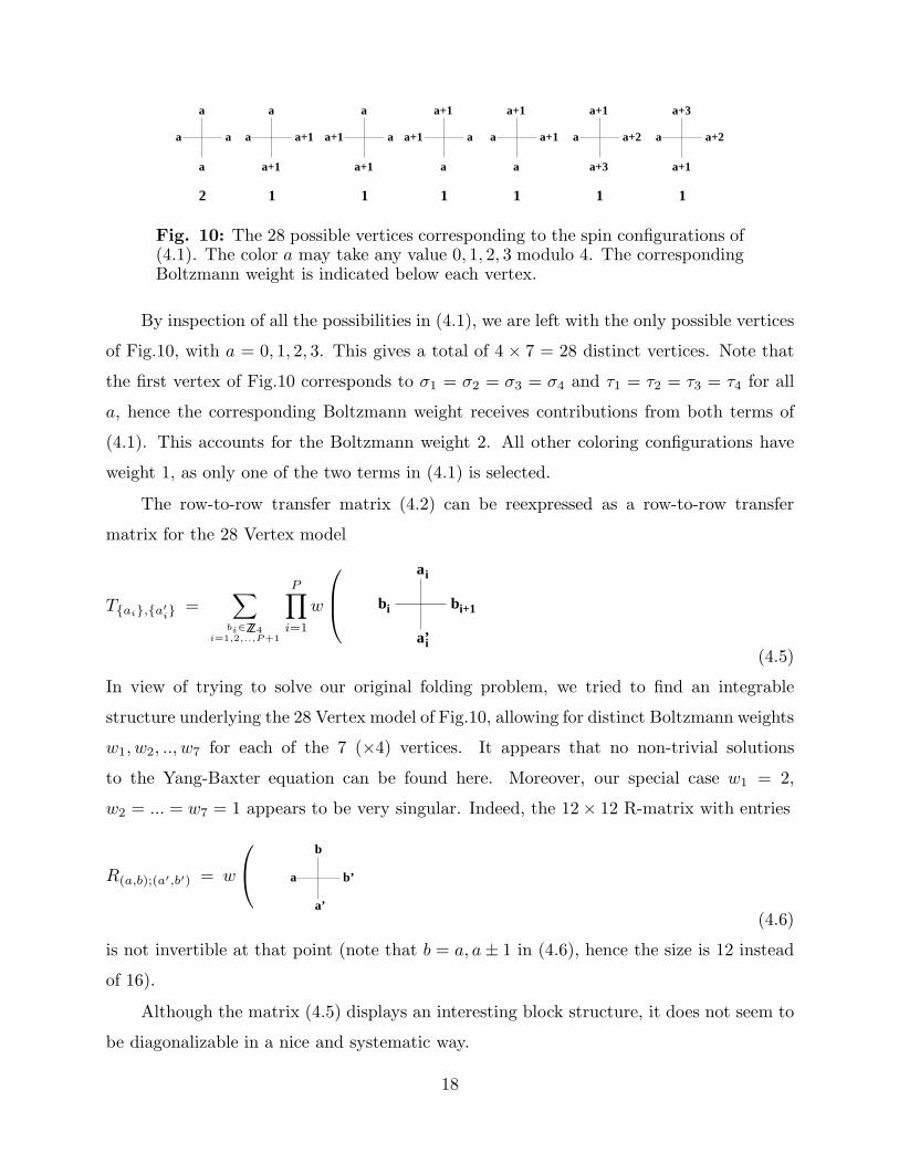
Fig. 10: The 28 possible vertices corresponding to the spin configurations of(4.1). The color a may take any value 0, 1, 2, 3 modulo 4. The correspondingBoltzmann weight is indicated below each vertex.

By inspection of all the possibilities in (4.1), we are left with the only possible vertices

of Fig.10, with a = 0, 1, 2, 3. This gives a total of 4 × 7 = 28 distinct vertices. Note that

the first vertex of Fig.10 corresponds to σ1 = σ2 = σ3 = σ4 and τ1 = τ2 = τ3 = τ4 for all

a, hence the corresponding Boltzmann weight receives contributions from both terms of

(4.1). This accounts for the Boltzmann weight 2. All other coloring configurations have

weight 1, as only one of the two terms in (4.1) is selected.

The row-to-row transfer matrix (4.2) can be reexpressed as a row-to-row transfer

matrix for the 28 Vertex model

T{ai},{a′i} =

∑

bi∈ZZ4i=1,2,..,P+1

P∏

i=1

w

a’i

bi+1

ai

bi

(4.5)

In view of trying to solve our original folding problem, we tried to find an integrable

structure underlying the 28 Vertex model of Fig.10, allowing for distinct Boltzmann weights

w1, w2, .., w7 for each of the 7 (×4) vertices. It appears that no non-trivial solutions

to the Yang-Baxter equation can be found here. Moreover, our special case w1 = 2,

w2 = ... = w7 = 1 appears to be very singular. Indeed, the 12× 12 R-matrix with entries

R(a,b);(a′,b′) = w

a’

b’a

b

(4.6)

is not invertible at that point (note that b = a, a± 1 in (4.6), hence the size is 12 instead

of 16).

Although the matrix (4.5) displays an interesting block structure, it does not seem to

be diagonalizable in a nice and systematic way.

18

5. Numerical Studies

This leaves us with little but the possibility of a numerical study, which we will carry

out in this section. This is particularly efficient because T is a sparse matrix. Indeed, there

are approximately 7N non-vanishing matrix elements in T (given the color of the western

edge of a vertex, there are exactly 7 possibilities for the northern, eastern and southern

edges), whereas T is a 4N ×4N matrix, hence a ratio of non-vanishing elements of (7/16)N .

The results of the following subsections have been obtained by

(i) constructing the transfer matrix T of the 28 Vertex model, including the appropriate

boundary conditions

(ii) determining the block structure of T

(iii) extracting the largest eigenvalue of T in the dominant block, by iteration of the action

of T on an initial vector v0, normalized at each step: this process converges nicely to

the Perron-Frobenius eigenvector of the matrix.

The particularity of the model gives us the possibility of generating the matrix ele-

ments of T ”linearly”, by simply listing all its non-vanishing entries (hence a list of length

≃ 7n). Indeed, for each sequence of n vertices in the list (each of which is chosen among

the 7 possibilities of Fig.10), the values of the bottom and top vertical edge images are

completely fixed. Conversely, a given pair (bottom,top) of vertical edge configurations

corresponds to at most one such arrangement of n vertices. This enables us to encode all

of T in a vector of length ≃ 7n, and to use it directly for determining the largest eigenvalue

λmax.

The various choices of boundary conditions are:

(1) periodic, by identifying the west-most and east-most edges of the row

(2) fixed, by setting to the value 0 both west-most and east-most edges of the row

(3) mixed, by fixing the east-most edge value to 0, and summing over all west-most edge

values. This latter case is also equivalent to having free boundary conditions on both

ends.

19

5.1. Periodic Boundary Conditions

n size λmax λ1/(4n)max

1 1 2. 1.18920

2 4 10. 1.33352

3 16 12.9282 1.23773

4 36 48.9317 1.27526

5 256 83.9919 1.24799

6 400 285.092 1.26558

7 4096 539.435 1.25189

Table I: Numerical results for the transfer matrix of the 28 Vertex modelwith periodic boundary conditions. We list the length n of the row, the size ofthe relevant block of the transfer matrix to be diagonalized, the largest eigen-

value λmax, and the sequence λ1/(4n)max , converging to the partition function per

triangle. Note the parity effect on this sequence, which gives a framing of theactual limit.

We display in Table I the results for the largest eigenvalue of the transfer matrix T for

periodic boundary conditions. We note the usual oscillatory behavior of the approximation

to the partition function per site, namely λ1/(4n)max . This makes extrapolation more difficult,

as we must distinguish between both parities of n, and we rather rely on the other types

of boundary conditions for a better behavior.

5.2. Fixed Boundary Conditions

n size λmax λ1/(4n)max νn

1 1 2.0000000 1.18920

2 3 4.5615528 1.20889 1.22891

3 7 10.898979 1.22025 1.24327

4 22 26.562737 1.22748 1.24945

5 69 65.399363 1.23247 1.25263

6 236 161.98393 1.23612 1.25451

7 800 402.76893 1.23890 1.25572

8 2850 1004.1851 1.24109 1.25657

20

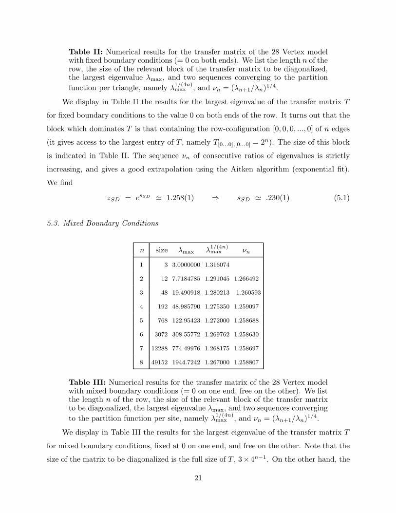
Table II: Numerical results for the transfer matrix of the 28 Vertex modelwith fixed boundary conditions (= 0 on both ends). We list the length n of therow, the size of the relevant block of the transfer matrix to be diagonalized,the largest eigenvalue λmax, and two sequences converging to the partition

function per triangle, namely λ1/(4n)max , and νn = (λn+1/λn)

1/4.

We display in Table II the results for the largest eigenvalue of the transfer matrix T

for fixed boundary conditions to the value 0 on both ends of the row. It turns out that the

block which dominates T is that containing the row-configuration [0, 0, 0, ..., 0] of n edges

(it gives access to the largest entry of T , namely T[0...0],[0...0] = 2n). The size of this block

is indicated in Table II. The sequence νn of consecutive ratios of eigenvalues is strictly

increasing, and gives a good extrapolation using the Aitken algorithm (exponential fit).

We find

zSD = esSD ≃ 1.258(1) ⇒ sSD ≃ .230(1) (5.1)

5.3. Mixed Boundary Conditions

n size λmax λ1/(4n)max νn

1 3 3.0000000 1.316074

2 12 7.7184785 1.291045 1.266492

3 48 19.490918 1.280213 1.260593

4 192 48.985790 1.275350 1.259097

5 768 122.95423 1.272000 1.258688

6 3072 308.55772 1.269762 1.258630

7 12288 774.49976 1.268175 1.258697

8 49152 1944.7242 1.267000 1.258807

Table III: Numerical results for the transfer matrix of the 28 Vertex modelwith mixed boundary conditions (= 0 on one end, free on the other). We listthe length n of the row, the size of the relevant block of the transfer matrixto be diagonalized, the largest eigenvalue λmax, and two sequences converging

to the partition function per site, namely λ1/(4n)max , and νn = (λn+1/λn)

1/4.

We display in Table III the results for the largest eigenvalue of the transfer matrix T

for mixed boundary conditions, fixed at 0 on one end, and free on the other. Note that the

size of the matrix to be diagonalized is the full size of T , 3× 4n−1. On the other hand, the

21

sequence νn of consecutive ratios of eigenvalues displays a very nice convergence. Using

the abovementioned extrapolation scheme, we arrive at

zSD = esSD ≃ 1.2586(1) ⇒ sSD ≃ .2299(1) (5.2)

Note that this result is slightly smaller than the Mayer estimate (2.13).

6. d-Dimensional Hypercubic-Diagonal Folding

6.1. Discrete Folding in Higher Dimensions

In the present paper, we have studied the two-dimensional folding of the square-

diagonal lattice, in which the image of the folding maps ρ is a subset of the original lattice.

If we relax the latter constraint, we may just consider maps from the original lattice to

say IRd. It is however desirable that the target configurations may only have finitely many

possibilities to form local folds, i.e. we should not allow folds with arbitrary angles. We

may introduce a higher-dimensional discrete folding problem by simply demanding that

the image of the folding maps ρ, subject to (2.2), be a subset of a d-dimensional lattice

[10]. This is possible only if the d-dimensional ”target” lattice is compatible with the

square-diagonal lattice, in the sense that such d-dimensional folding configurations indeed

exist.

B

A

B

A

Fig. 11: The unit cell of the Hypercubic-Diagonal lattice of dimension d = 3.The horizontal plane sections alternate between the A and B types of square-diagonal lattice as we move along the vertical. This holds for any other planesections perpendicular to a basis vector.

We have found two such compatible choices of lattice. The first choice consists of

the d-dimensional Hypercubic-Diagonal (d-HCD) lattice (represented in Fig.11 for d = 3),

generated by the orthonormal vectors ~e1, ~e2, ..., ~ed, |~ei| = 1 (with ”short” edges of length

1), together with exactly one of the diagonals on each of its 2-dimensional faces (the ”long”

22

edges, of length√2). These diagonals are chosen so that none of them contains the origin of

the lattice, and that each plane section of the lattice, parallel say to (~ei, ~ej), 1 ≤ i < j ≤ d,

is a copy of the square-diagonal lattice, with an alternance of A and B-types (c.f. Fig.11)

as we move along a direction ~ek, perpendicular to (~ei, ~ej). Note that on the lattice, any

two short edges are either parallel or perpendicular. The sub-lattice of the HCD formed by

erasing all short edges was also considered for the d-dimensional folding of the triangular

lattice in [10].

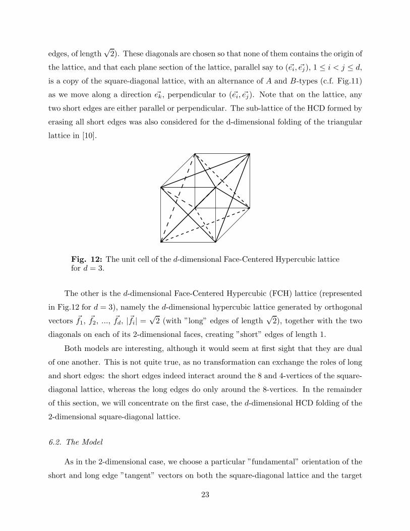
Fig. 12: The unit cell of the d-dimensional Face-Centered Hypercubic latticefor d = 3.

The other is the d-dimensional Face-Centered Hypercubic (FCH) lattice (represented

in Fig.12 for d = 3), namely the d-dimensional hypercubic lattice generated by orthogonal

vectors ~f1, ~f2, ..., ~fd, |~fi| =√2 (with ”long” edges of length

√2), together with the two

diagonals on each of its 2-dimensional faces, creating ”short” edges of length 1.

Both models are interesting, although it would seem at first sight that they are dual

of one another. This is not quite true, as no transformation can exchange the roles of long

and short edges: the short edges indeed interact around the 8 and 4-vertices of the square-

diagonal lattice, whereas the long edges do only around the 8-vertices. In the remainder

of this section, we will concentrate on the first case, the d-dimensional HCD folding of the

2-dimensional square-diagonal lattice.

6.2. The Model

As in the 2-dimensional case, we choose a particular ”fundamental” orientation of the

short and long edge ”tangent” vectors on both the square-diagonal lattice and the target

23

d-dimensional HCD lattice, and consider the set of folding configurations of the square-

diagonal lattice into the d-dimensional target lattice, namely the set of distinct images of

folding maps ρ subject to the constraint (2.2) around each face of the original lattice.

The target short edges may take only 2d distinct values, namely ±~e1, ±~e2, ..., ±~ed,

where ~e1, ...,~ed denotes the orthonormal basis of the d-dimensional hypercubic lattice. The

target long edges may take only 2d(d−1) distinct values, namely ±~ei± ~ej for 1 ≤ i < j ≤ d.

The image of a given short tangent vector ~t of the original lattice reads

ρ(~t) = ǫ~ei (6.1)

hence is characterized by a ”color” i ∈ {1, 2, ..., d} and a sign ǫ = ±1.

In a folding configuration, there are basically only two relative possibilities for the

images of the tangent vectors to two adjacent faces sharing a long edge. Indeed, given the

values ~u = ǫ~ei, ~v = η~ej , i 6= j, of the two short edges of the image of the first triangle,

there are only two possibilities for the images ~u′, ~v′ of the two short edges of the second

triangle: the face rule (2.2) imposes that ~u′ + ~v′ = ~u+ ~v, which holds if and only if

~u′ = ~u = ǫ~ei and ~v′ = ~v = η~ej

or ~u′ = ~v = η~ej and ~v′ = ~u = ǫ~ei(6.2)

This leaves us again with the only two possibilities of (2.4). As a corollary, the long edge

adjacent to the two triangles is always either completely folded, or unfolded.

Let us now investigate the folding configurations of short edges. The two triangles

adjacent to a short edge have images of the form

jeε

η ie

keσ

(6.3)

where i 6= j and i 6= k.

This gives rise to essentially four types of foldings for the short edge, as depicted in

Fig.13. If j = k, the short edge is completely folded (180◦) when σ = η and unfolded

when σ = −η. If j 6= k, the long edge is always folded at a right angle, either up or down

according to the relative values of ǫ, σ and η.

24

. . ..

Fig. 13: The four types of folds of the short edge separating two triangles inthe d-HCD model: complete fold, no fold, right angle up, right angle down.The figure is drawn in the space spanned by ~ei, ~ej , ~ek of (6.3).

6.3. Equivalent Loop model

The only constraint coming from the face rule (2.2) on a given triangle is that the two

short edges should have perpendicular images, of the form ±~ei and ±~ej respectively, with

1 ≤ i 6= j ≤ d, namely that they be painted with different colors i and j.

A folding configuration of the square-diagonal lattice in d dimensions amounts to a

coloring of all the short edges with colors i = 1, 2, ..., d, and a choice of signs ǫ = ±1, which

propagate along each loop of a given color (according to (6.2)).

j

i

k

l

Fig. 14: The ”dual” coloring of the faces of S in the d-HCD model. Theformer short and long edges are represented in thin solid lines. The new edgeshave the same colors i, j, k, l as the short edges they intersect.

To best see this, let us consider the square-diagonal lattice, together with its square

sub-lattice S, whose vertices are those of valency 8 in the original lattice. The lattice S

has therefore long edges, and each of its faces is made of 4 former triangles, hence has

4 short edges along its diagonals. Let us replace the coloring of the short edges by that

of ”dual” edges linking the midpoints of the edges of S around its faces, as illustrated in

25

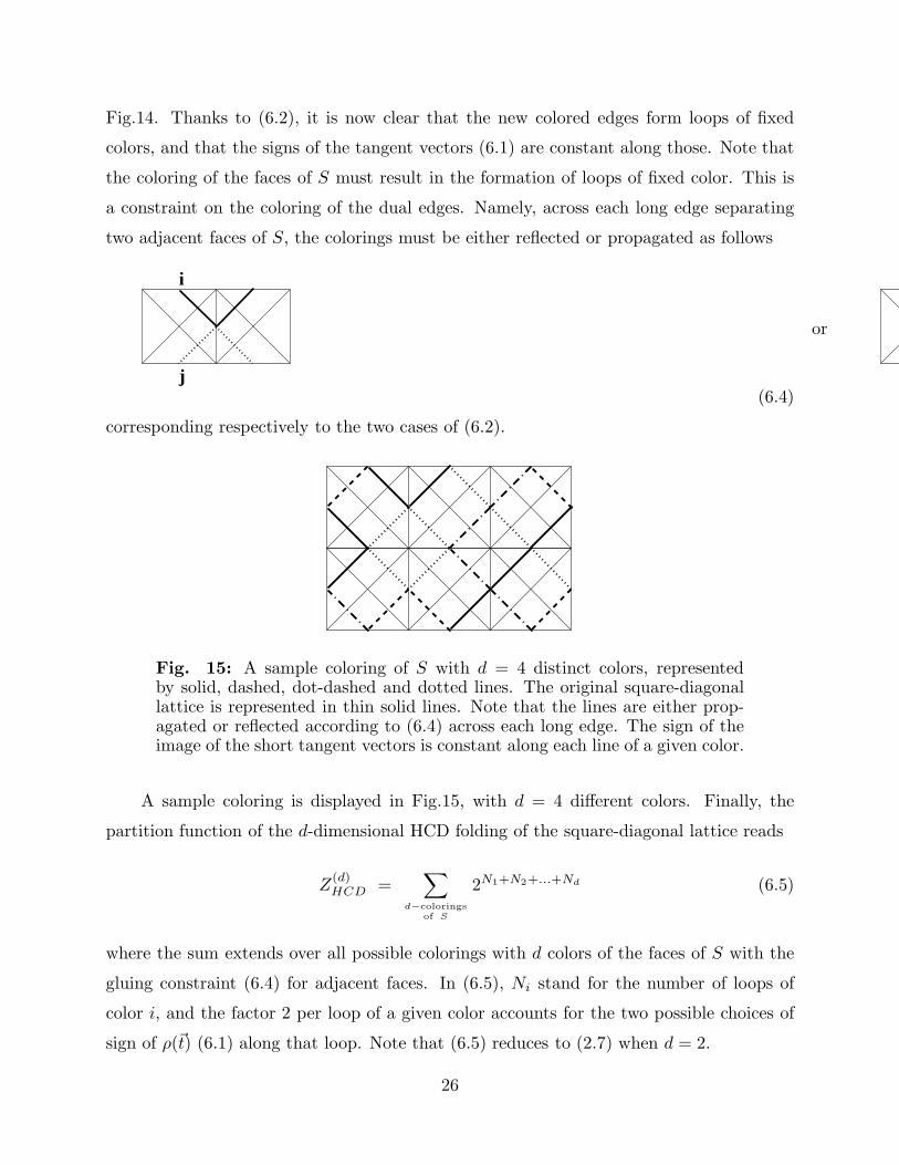
Fig.14. Thanks to (6.2), it is now clear that the new colored edges form loops of fixed

colors, and that the signs of the tangent vectors (6.1) are constant along those. Note that

the coloring of the faces of S must result in the formation of loops of fixed color. This is

a constraint on the coloring of the dual edges. Namely, across each long edge separating

two adjacent faces of S, the colorings must be either reflected or propagated as follows

j

i

or

(6.4)

corresponding respectively to the two cases of (6.2).

Fig. 15: A sample coloring of S with d = 4 distinct colors, representedby solid, dashed, dot-dashed and dotted lines. The original square-diagonallattice is represented in thin solid lines. Note that the lines are either prop-agated or reflected according to (6.4) across each long edge. The sign of theimage of the short tangent vectors is constant along each line of a given color.

A sample coloring is displayed in Fig.15, with d = 4 different colors. Finally, the

partition function of the d-dimensional HCD folding of the square-diagonal lattice reads

Z(d)HCD =

∑

d−colorings

of S

2N1+N2+...+Nd (6.5)

where the sum extends over all possible colorings with d colors of the faces of S with the

gluing constraint (6.4) for adjacent faces. In (6.5), Ni stand for the number of loops of

color i, and the factor 2 per loop of a given color accounts for the two possible choices of

sign of ρ(~t) (6.1) along that loop. Note that (6.5) reduces to (2.7) when d = 2.

26

6.4. Estimates for the d-HCD Folding Entropy

The expression (6.5) for the partition function of the d-dimensional HCD folding of

the square-diagonal lattice provides us with upper and lower bounds on the entropy.

First of all, note that

Z(d)HCD ≤ Z

(d+1)HCD (6.6)

as Z(d)HCD is a partial sum of Z

(d+1)HCD corresponding to no loop of color d + 1 (Nd+1 = 0).

This shows that all the corresponding thermodynamic entropies s(d)HCD are non-zero for

d ≥ 2.

To find a lower bound on s(d)HCD, let us try to expand (6.5) around one of its ”fun-

damental” states maximizing the total number of loops N1 + ... + Nd = N/4. Note that

there are as many such states as d-colorings of the vertices of S with colors 1, 2, ..., d and

such that no two adjacent vertices have same color. Indeed, a fundamental state is made

of loops of minimal length 4 surrounding each vertex of S such that any two neighboring

loops have distinct colors, hence the loop configuration is equivalent to a vertex-coloring.

For these fundamental configurations, we have a first rough estimate of Z(d)HCD (actually a

lower bound) in the form

Z(d)HCD ≥ 2N/4 ZS(d) (6.7)

where ZS(d) denotes the number of d-colorings of the vertices of S. This is the lead-

ing order of the Mayer expansion of the partition function. The d-coloring entropy

sS(d) = limN→∞ Log(ZS(d))/N is known exactly in the thermodynamic limit only for

d = 2 and 3. As we already pointed out, there are indeed only two groundstates at d = 2,

i.e. ZS(2) = 2, and the thermodynamic entropy per site is sS(2) = 0: (6.7) then leads

to (2.9). For d = 3, the 3-coloring problem of the vertices of the square lattice S (or

equivalently of the faces of its dual S∗) is equivalent to the ice model [12], with an entropy

per site

sS(3) =3

2Log(

4

3) (6.8)

This gives the lower bound for d = 3

s(3)HCD ≥ 1

4Log 2 +

1

4sS(3) = Log 2− 3

8Log 3 = .281167... (6.9)

or a partition function per triangle of 1.32467...

Let us estimate the lower bound (6.7) when d is large. As a very rough leading

approximation, each vertex of S can be painted with one of d colors, minus the small

27

number of colors used for its neighbouring vertices, hence if d is very large, we have

ZS(d) ≃ dN/4. This gives the leading estimate

s(d)HCD ≃ 1

4Log(2d) (6.10)

A more careful study shows that this is accurate up to the order of 1/d.

6.5. Vertex Model

As in the d = 2 case, let us transform the colored loop model of Sect.6.3 into a vertex

model, by mapping the coloring configurations and sign choices on each face of S onto

Vertex configurations for the dual square lattice S∗. Each colored new edge on the faces of

S has been assigned a color i ∈ {1, 2, ..., d} and a sign ǫ ∈ {−1, 1} (see Fig.14), which are

conserved (either propagated or reflected, according to (6.4)) at each crossing of an edge

of S. This suggests to attach to each edge of S∗ a pair of colors and signs (i, σ; j, τ), with

say 1 ≤ i < j ≤ d. This gives 2d(d− 1) possible values for this edge variable. The vertex

model is then defined by the list of all possible edge configurations around a vertex of S∗,

together with the gluing property that each edge of S∗ has a well-defined configuration.

Each allowed vertex has Boltzmann weight 1.

Let us count the number of allowed vertices for generic values of d. This is the same

as the number of coloring and sign configurations on each face of S. To count the latter,

note that the only constraint on the four color/sign pairs (i1, σ1), ..., (i4, σ4) is that any

two consecutive colors must be distinct. So we merely have to count the number of cyclic

arrangements of four colors taken among d around the face. Introducing the d×d matrices

I and J , with entries Ii,j = δi,j , and Ji,j = 1 for all i, j, the total number of vertices reads

Vd = 16Tr(J − I)4 = 16d(d− 1)(d2 − 3d+ 3) (6.11)

where we have used the relation J2 = dJ , and factored out the contribution 16 for the

independent choices of the four signs.

Note that (6.11) yields V2 = 32 instead of 28, for d = 2. This is because we must keep

track of the edge colors as soon as d > 2. At d = 2, the model has been further simplified

by noticing that any reference to the edge coloring could be omitted, at the expense of

modifying the Boltzmann weights (four vertices actually acquired a Boltzmann weight 2).

The row-to-row transfer matrix of the vertex model is again sparse. Indeed, if we

fix the value of the west-most edge in a row of N vertices, we have a number of non-

vanishing matrix elements of the order of (Vd/(2d(d − 1)))N , whereas the matrix has a

total of (2d(d − 1))2N elements, hence a ratio [2(d2 − 3d + 3)/(d2(d − 1)2)]N , which gets

smaller as d increases.

28

6.6. Numerical Study

In this section, we extract some numerical estimates for the HCD folding entropy in

dimension d = 3, from the largest eigenvalue of the transfer matrix of the 288 Vertex model

described in the previous section.

n λmax νn

1 2.000000

2 5.587741 1.29286

3 17.11799 1.32298

4 54.54084 1.33603

5 177.4631 1.34306

Table IV: Numerical results for the transfer matrix of the V3 = 288 Vertexmodel with fixed boundary conditions ( =(1,+; 2,+) on both ends) for the3-dimensional HCD folding. We have represented the size n of the row, thelargest eigenvalue and the ratio νn = (λn+1/λn)

1/4, which converges to thepartition function per triangle.

We are indeed limited by the rapid growth of the size of the transfer matrix, and more

importantly of its number of non-vanishing entries, which grows like (8(d2 − 3d+ 3))n for

a row of width n. At d = 3, this is already 24n, and we have been only able to consider

transfer matrices up to the width n = 5, with fixed boundary conditions (with the edge

variables fixed to (i, σ; j, τ) = (1,+; 2,+) on both ends).

The results for the largest eigenvalue of the corresponding transfer matrix of the 288

Vertex model are displayed in Table IV, together with the sequence νn = (λmax(n +

1)/λmax(n))1/(4n), converging to the partition function per triangle z

(3)HCD. The extrapo-

lated thermodynamic entropy reads

s(3)HCD ≃ .300.. (6.12)

or a partition function per triangle z(3)HCD ≃ 1.35(1) Note that our estimate (6.12) agrees

with the lower bound (6.9).

7. d-Dimensional FCH Folding

7.1. The Model

As in the 2-dimensional case, we choose a particular ”fundamental” orientation of the

short and long edge ”tangent” vectors of the d-HCD lattice of Fig.12, and consider the set

29

of folding configurations of the square-diagonal lattice into the d-dimensional FCH lattice,

namely the set of distinct images of folding maps ρ subject to the constraint (2.2) around

each face of the original lattice.

The target long edges may take only 2d distinct values, namely ±~f1, ±~f2, ..., ±~fd,

where ~f1, ..., ~fd form an orthogonal basis of IRd (with |~fi| =√2 for all i). The target short

edges may take only 2d(d − 1) distinct values, namely the unit vectors (±~fi ± ~fj)/2 for

1 ≤ i < j ≤ d.

In a folding configuration, there are many possibilities for the images of the tangent

vectors to two adjacent faces sharing a long edge, namely

- jfε

- ifjf η )/2

ifηjf + )/2 jf kfσ+

kfσjf -ε

ε

(

( ε(

ε( )/2

)/2

(7.1)

where i, j, k ∈ {1, 2, ..., d}, i and k distinct from j, and ǫ, η, σ are arbitrary signs.

. . ..

Fig. 16: The four types of folds of the long edge separating two triangles inthe d-FCH model: complete fold, no fold, right angle up, right angle down.

The figure is drawn in the space spanned by ~fi, ~fj, ~fk of (7.1).

This gives rise to essentially four types of foldings for the long edge, as depicted in

Fig.16. If i = k, the long edge is completely folded (180◦) when σ = η and unfolded when

σ = −η. If i 6= k, the long edge is always folded at a right angle, either up when σ = η

(+90◦), or down if σ = −η (−90◦).

7.2. Vertex Model

Let us again consider the square lattice S whose vertices are the 8-valent vertices

of the square-diagonal lattice. The edges of S are the long edges of the original lattice.

30

According to the previous section, these edges are folded into edges of the form

ρ(~t) = ǫ~fi (7.2)

Each such image is therefore characterized by a color i ∈ {1, 2, ..., d} and a sign ǫ ∈ {−1, 1}.Let us examine the possible relative images of the long edges in two triangles sharing a

short edge. There are basically only two possibilities

jfifε σ

jfσ- )/2ifε(-

or

fε

(7.3)

to accomodate the face rule (2.2), where i 6= j, i 6= k, and ǫ, σ, η are arbitrary signs.

We have indicated only the value of the central short edge image, as the remaining ones

are immediately deduced from the face rule (2.2). As a corollary, we see that the short

edges are always either completely folded (solid line in (7.3)), or unfolded (dashed line

in (7.3)). Together with Fig.16, this shows a complete parallel between the d-HCD and

d-FCH models: we see that the roles of the long and short edges are exchanged in the two

models, at least as far as the types of folding are concerned. Note however that there are

twice as many short edges as long edges in the square-diagonal lattice, we therefore expect

a difference in the folding entropies of the two models.

ej

eiεej

eiε

σ

σ ej

ejeiε

eiε

σ

σ

eiε

eiεeiε

eiε

eiε

ej

eiε

-

ejσσ -

number of vertices

weight

4d(d-1) 4d(d-1) 4d(d-1)2d

2(d-1) 1 1 1

Fig. 17: The allowed configurations of long edges around a face of S in thed-FCH model. We have indicated the degeneracy of each face configurationand the corresponding Boltzmann weight. The inner short lines represent thestate of the corresponding short edges, namely completely folded (solid line)or unfolded (dashed line).

Let us now investigate the possible configurations of the images of the long edges

around a face of S. Using (7.3) and proceeding by inspection, we have found the face

configurations displayed in Fig.17, together with their degeneracy and attached Boltzmann

31

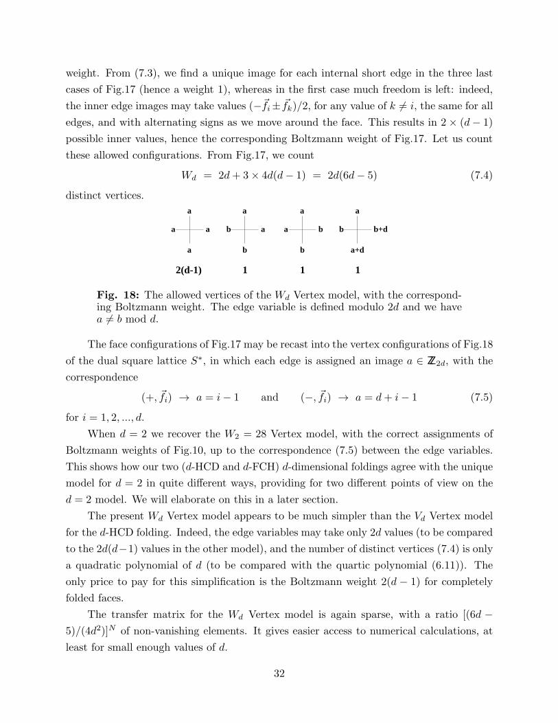
weight. From (7.3), we find a unique image for each internal short edge in the three last

cases of Fig.17 (hence a weight 1), whereas in the first case much freedom is left: indeed,

the inner edge images may take values (−~fi± ~fk)/2, for any value of k 6= i, the same for all

edges, and with alternating signs as we move around the face. This results in 2× (d− 1)

possible inner values, hence the corresponding Boltzmann weight of Fig.17. Let us count

these allowed configurations. From Fig.17, we count

Wd = 2d+ 3× 4d(d− 1) = 2d(6d− 5) (7.4)

distinct vertices.

1 1

a

a

a

aa b b+d

2(d-1)

a

b

b

a+d

a

1

a

b a

b

Fig. 18: The allowed vertices of the Wd Vertex model, with the correspond-ing Boltzmann weight. The edge variable is defined modulo 2d and we havea 6= b mod d.

The face configurations of Fig.17 may be recast into the vertex configurations of Fig.18

of the dual square lattice S∗, in which each edge is assigned an image a ∈ ZZ2d, with the

correspondence

(+, ~fi) → a = i− 1 and (−, ~fi) → a = d+ i− 1 (7.5)

for i = 1, 2, ..., d.

When d = 2 we recover the W2 = 28 Vertex model, with the correct assignments of

Boltzmann weights of Fig.10, up to the correspondence (7.5) between the edge variables.

This shows how our two (d-HCD and d-FCH) d-dimensional foldings agree with the unique

model for d = 2 in quite different ways, providing for two different points of view on the

d = 2 model. We will elaborate on this in a later section.

The present Wd Vertex model appears to be much simpler than the Vd Vertex model

for the d-HCD folding. Indeed, the edge variables may take only 2d values (to be compared

to the 2d(d−1) values in the other model), and the number of distinct vertices (7.4) is only

a quadratic polynomial of d (to be compared with the quartic polynomial (6.11)). The

only price to pay for this simplification is the Boltzmann weight 2(d − 1) for completely

folded faces.

The transfer matrix for the Wd Vertex model is again sparse, with a ratio [(6d −5)/(4d2)]N of non-vanishing elements. It gives easier access to numerical calculations, at

least for small enough values of d.

32

2(d-1) 1 11

Fig. 19: The four types of colored vertices for the d-FCH folding model.The solid and dashed lines stand for any two distinct colors in {1, 2, ..., d}.The signs are conserved along colored lines, except for the last vertex, wherethey are reversed.

7.3. Loop Model

The Wd Vertex model of the previous section can be refined as follows. Let us dis-

entangle the sign and color variables on each edge of S∗, and represent only the color of

the edge, by painting it accordingly. This leaves us with only the four types of vertices

depicted in Fig.19. the signs must now be conserved or reversed along colored lines ac-

cording to Fig.17. The sign is actually conserved in all cases, except when the two lines of

different color cross each other (last, completely unfolded case of Fig.17), in which case it

is reversed. These colored lines form loop-like clusters, along which the signs are entirely

determined by their value on one of the edges of the cluster. Moreover, all values are

compatible, as there are always an even number of sign reversals (due to an even number

of crossings with lines of other colors) along a loop.

Fig. 20: A sample coloring configuration for the d-FCH folding model, ford = 4.

33

Hence on top of the Boltzmann weights indicated in Fig.19, we must include a weight

2 per loop-like cluster of given color. A sample configuration of the model for d = 4

is displayed in Fig.20 for illustration. With free boundary conditions, this configuration

would receive the weight 27 × 2(4− 1) = 1536, as 7 colored clusters are formed, and one

vertex is of the first type of Fig.19.

7.4. Estimates for the d-FCH Folding Entropy

The loop model of previous section permits to derive lower bounds on the partition

function Z(d)FCH of the d-FCH folding model, henceforth on the d-FCH folding entropy.

We first note that there are exactly 2d fundamental configurations of the loop model

with minimum energy (i.e. maximum Boltzmann weight), namely those obtained with

only the first vertex of Fig.18, that is where all the edges are painted with the same color.

The contribution to the partition function of each of these groundstates is [2(d − 1)]n

for a portion of S∗ with n vertices. Using Fig.17, these correspond to completely folded

configurations of all the short edges.

(a) (b)

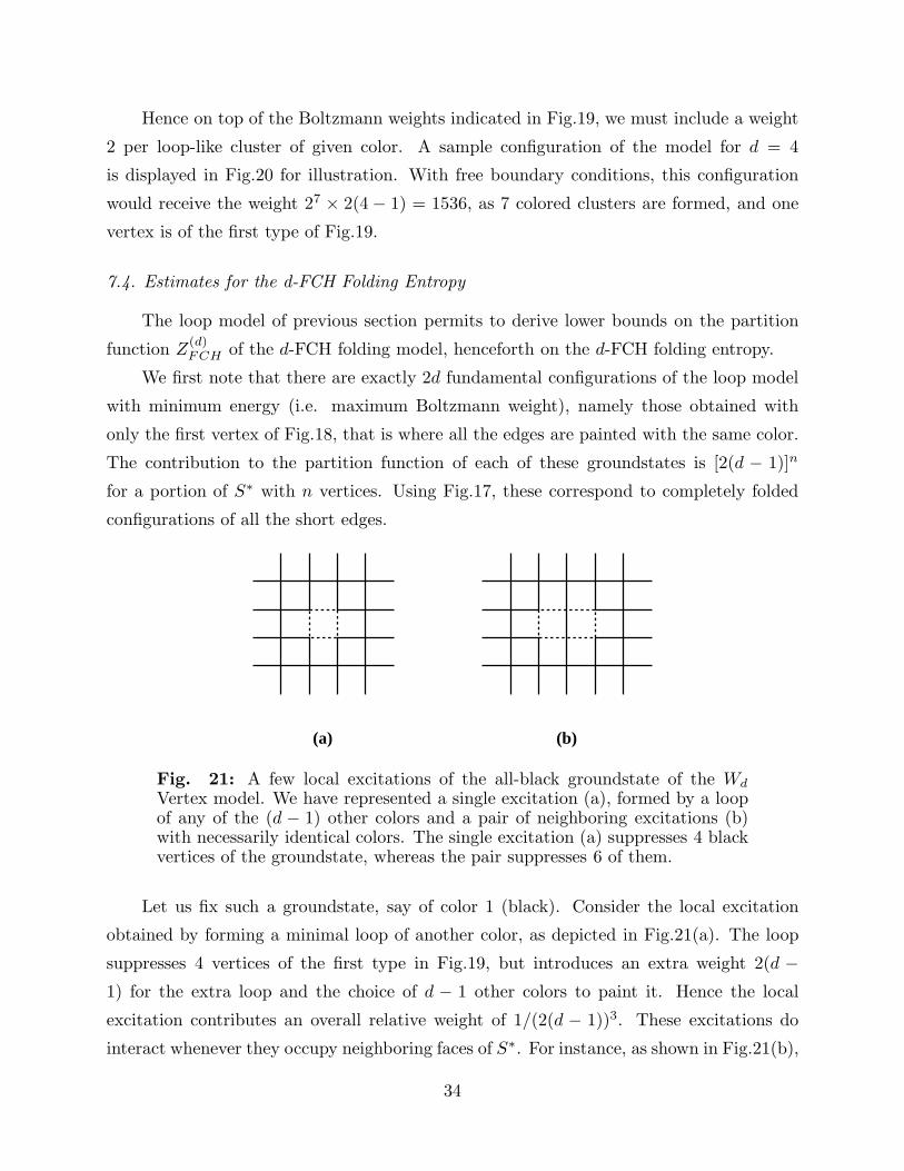
Fig. 21: A few local excitations of the all-black groundstate of the Wd

Vertex model. We have represented a single excitation (a), formed by a loopof any of the (d − 1) other colors and a pair of neighboring excitations (b)with necessarily identical colors. The single excitation (a) suppresses 4 blackvertices of the groundstate, whereas the pair suppresses 6 of them.

Let us fix such a groundstate, say of color 1 (black). Consider the local excitation

obtained by forming a minimal loop of another color, as depicted in Fig.21(a). The loop

suppresses 4 vertices of the first type in Fig.19, but introduces an extra weight 2(d −1) for the extra loop and the choice of d − 1 other colors to paint it. Hence the local

excitation contributes an overall relative weight of 1/(2(d − 1))3. These excitations do

interact whenever they occupy neighboring faces of S∗. For instance, as shown in Fig.21(b),

34

two such neighboring excitations are forced to have the same color, and form only one extra

loop, whereas they suppress 6 vertices of the first type in Fig.19. Hence, instead of the

expected relative weight 1/(2(d− 1))6, they only contribute for (2(d − 1))/(2(d− 1))6 =

1/(2(d− 1))5. This propagates to higher numbers of excitations. In general, the partition

function is underestimated if we neglect these interactions. This provides us with an exact

lower bound

Z(d)FCH ≥

[

2(d− 1)(1 +1

(2(d− 1))3)

]n

(7.6)

hence

s(d)FCH ≥ 1

4Log

(

2(d− 1)(1 +1

(2(d− 1))3)

)

(7.7)

d entropy p. func.

2 .20273255 1.224744

3 .35044964 1.419705

4 .44909460 1.566892

5 .52034819 1.682613

6 .57589615 1.778723

7 .62137130 1.861478

8 .65985542 1.934512

9 .69320821 2.000122

10 .72263580 2.059855

Table V: Lower bound on the d-dimensional FCH folding entropy, from (7.7).We display the dimension d, the lower bound on the folding entropy and thecorresponding lower bound on the partition function per triangle.

The values of the lower bound (7.7) for the d-FCH model are displayed in Table V.

Note that (7.7) consists of the two leading orders of the Mayer expansion of Z(d)FCH in

terms of the local excitations described above. The expansion however is quite involved,

as the excitations interact between nearest neighbours (two faces sharing an edge) and

second-nearest neighbors (two faces sharing a vertex) as well. In the latter case, we have

to use extra caution and distinguish between the cases when the two excitations have the

same or different colors. Up to order 2 in these excitations, we find

(

Z(d)FCH

)1n = u(1 +

1

u3+

5

u5− 8

u6+O(

1

u7)) (7.8)

35

where we have set u = 2(d − 1). Note the bad apparent convergence at d = 2 (u = 2),

where this yields z ≃ 1.233, way below our best estimate 1.258. It appears that for d = 2

the Mayer expansion (2.13) around a very different groundstate is much more accurate.

So, although both have the same contribution 2n to the partition function, the latter

groundstate yields better corrections. This competition between different groundstates

could yield an interesting phase diagram for a fully interacting model.

We expect however the expansion (7.8) to behave better for larger values of d, for

which the existence of a groundstate generalizing that leading to (2.13) is not clear.

Comparing (7.7) to the large d estimate (6.10) for the HCD model, we conclude that

the two d-dimensional folding models (HCD and FCH) agree in the large d limit.

7.5. Numerical Study

In view of the previous sections, the Wd Vertex model is a straightforward generaliza-

tion of the 28 Vertex model we have already studied. A direct adaptation of our programs

permits to calculate the largest eigenvalue of the transfer matrix for a few values of d.

Like in the d = 2 case, we use the method of iteration of the action of the transfer

matrix T on a given vector, which we normalize at each step. To construct T , we simply list

its (6d−5)n non-zero elements, for fixed boundary conditions (say = 0) on the leftmost edge

of the row. Each such element has a unique pair of (row,column) indices in T : indeed, the

type of vertex in Fig.18 is fixed uniquely whenever the east, north and south edge variables

are given. Like in the d = 2 case, this linear description of the matrix gives access to large

sizes. We list our results in Table VI below, for fixed boundary conditions (= 0) on both

ends.

36

n λmax νn n λmax νn

1 4.0000000 1 6.0000000

d = 3 2 16.271109 1.420166 d = 4 2 36.170708 1.566936

3 67.253188 1.425850 3 218.18854 1.567179

W3 = 78 4 280.96435 1.429666 W4 = 152 4 1316.2983 1.567222

5 1185.8001 1.433309 5 7941.2213 1.567231

6 5063.2725 1.437490

1 8.0000000 1 10.000000

d = 5 2 64.127762 1.682631 d = 6 2 100.10133 1.778729

3 514.66822 1.683140 3 1002.5120 1.778944

W5 = 250 4 4131.2200 1.683207 W6 = 372 4 10040.689 1.778969

5 33162.598 1.683226

Table VI: Numerical results for the transfer matrix of the Wd Vertex modelwith fixed boundary conditions (= 0 on both ends). We list the dimension d,

the length n of the row, the largest eigenvalue λmax, and the sequence λ1/(4n)max ,

and νn = (λn+1/λn)1/4, converging to the partition function per triangle.

These values are extrapolated to the following

s(3)FCH = .378... z

(3)FCH = 1.47...

s(4)FCH = .4493... z

(4)FCH = 1.5672...

s(5)FCH = .5207... z

(5)FCH = 1.6832...

s(6)FCH = .57603... z

(6)FCH = 1.77896...

(7.9)

for the entropy sFCH and the partition function per triangle zFCH . Note the excellent

agreement with the lower bounds of Table V, for d = 4, 5, 6. We expect the Mayer expansion

(7.8) to be an excellent approximation to the partition function per site for all d ≥ 4.

37

n λmax νn

1 5.000000

2 24.21917 1.48353

3 119.4202 1.49014

4 582.3144 1.48600

5 2812.592 1.48247

6 13498.13 1.48010

Table VII: Numerical results for the transfer matrix of the W3 Vertex modelwith mixed boundary conditions (= 0 on one end, free on the other) for the3-dimensional FCH folding. We have represented the size n of the row, thelargest eigenvalue and the ratio νn = (λn+1/λn)

1/4, which converges to thepartition function per triangle.

For d = 3, we observe a much slower convergence (see Table VI). To obtain better

results, we have also calculated the largest eigenvalue of the transfer matrix T in the case

of mixed boundary conditions, fixed at 0 on one end, and free on the other. The results

are displayed in Table VII. Upon extrapolation, this leads to a more precise result for the

3-dimensional FCH folding entropy and partition function per triangle:

s(3)FCH ≃ .3854... z

(3)FCH ≃ 1.470.. (7.10)

8. Other Compactly Foldable Lattices

8.1. Classification of Compactly Foldable Lattices

We would like to briefly address the following question: can one classify the inequiva-

lent two-dimensional lattices which are compactly foldable onto themselves in two dimen-

sions? By this we mean that all maps ρ preserving the face rule (2.2) and the lengths of

edges, and with values in IR2 actually have their image included in the original lattice.

Another formulation is the existence of a map ρ whose image is a single face of the lattice

(the lattice is then completely foldable onto that face).

We already know of three examples: the square lattice (and its trivial variation the

rectangular lattice), the regular triangular lattice and the square-diagonal lattice intro-

duced in this paper.

38

Fig. 22: The square-diagonal lattice as the superposition of two squarelattices S and S′. The edges of S are represented in solid lines, those of S′ indashed lines.

Fig. 23: The dilation/rotation transformation on the triangular lattice givesrise to another triangular lattice represented in dashed lines. The superpo-sition of the two forms a new foldable lattice, with long, medium and shortedges.

One way to look at the square-diagonal lattice is rather as the superposition of two

square lattices (see Fig.22), say S and S′, such that S′ is a dilated version of S by a factor√2 as well as rotated by 45◦, so that the vertices of S′ coincide with half of the vertices of

S, forming a checkerboard.

This suggests to apply the same type of transformation (dilation/rotation) to the

triangular lattice. The only non-trivial possibility is a dilation by a factor of√3, and

a rotation by 30◦, displayed in Fig.23. This gives rise to a new foldable lattice in two

dimensions, by superposition of the two triangular lattices, called the double-triangular

lattice. We expect its entropy of two-dimensional folding to be larger than that of the

square-diagonal model. This model will be studied in the next section.

This can be shown to actually exhaust all the possibilities for compactly foldable two-

dimensional lattices. As a side remark, the generating function for compactly foldable

random triangulations of arbitrary genus was obtained in [13].

39

8.2. Two-Dimensional Folding of the Double-Triangular Lattice

The double-triangular lattice of Fig.23 has three types of edges: long, medium, short

of respective lengths 2,√3, 1. Each triangular face has one edge of each type. As usual,

we introduce tangent vectors along these edges, with compatible orientations throughout

the lattice, so that the face rule (2.1) is satisfied around each triangular face.

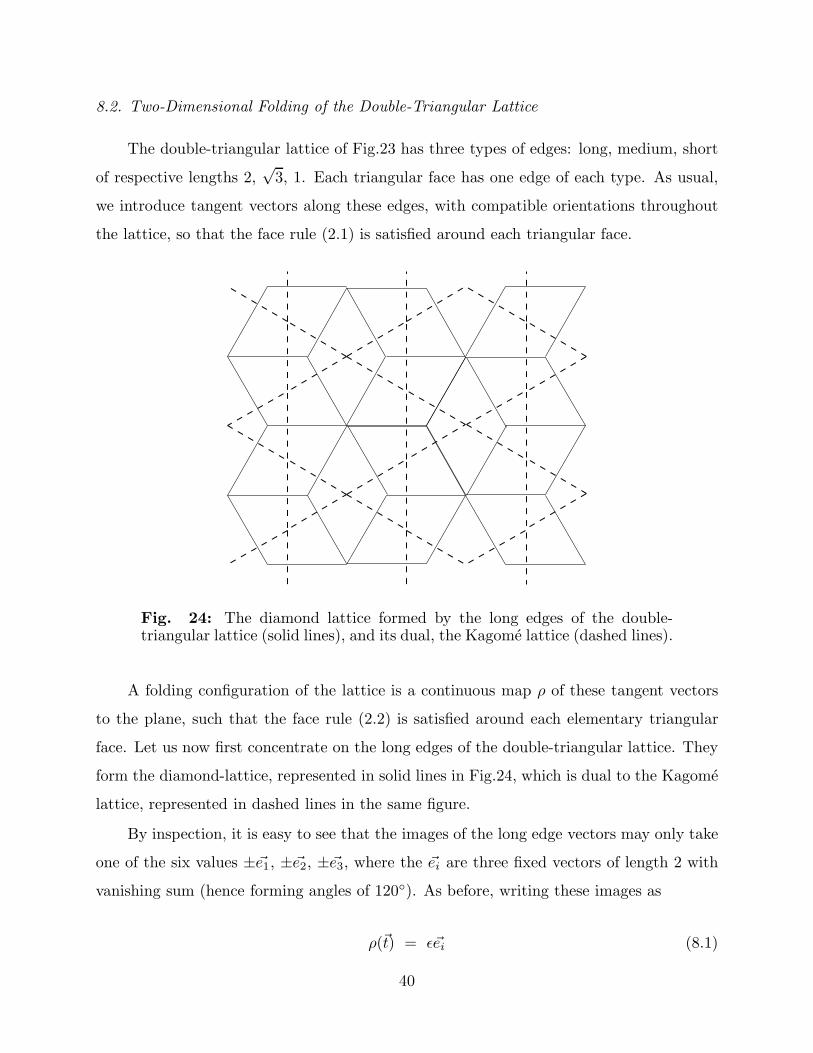
Fig. 24: The diamond lattice formed by the long edges of the double-triangular lattice (solid lines), and its dual, the Kagome lattice (dashed lines).

A folding configuration of the lattice is a continuous map ρ of these tangent vectors

to the plane, such that the face rule (2.2) is satisfied around each elementary triangular

face. Let us now first concentrate on the long edges of the double-triangular lattice. They

form the diamond-lattice, represented in solid lines in Fig.24, which is dual to the Kagome

lattice, represented in dashed lines in the same figure.

By inspection, it is easy to see that the images of the long edge vectors may only take

one of the six values ±~e1, ±~e2, ±~e3, where the ~ei are three fixed vectors of length 2 with

vanishing sum (hence forming angles of 120◦). As before, writing these images as

ρ(~t) = ǫ~ei (8.1)

40

eε i

eiε

ieε

eiε

eiεeiε

eiε

ejσ ejσejσ

eiε

- ejσ

eiε ejσ ejσ eiε-

1 1 12

Fig. 25: The four possible configurations of long edges around a diamond-shaped face. We have represented in dashed lines the (medium or short)unfolded inner edges, and in solid lines the folded inner edges. We have alsoindicated the attached Boltzmann weights. The color indices take the valuesi, j = 1, 2, 3, with i 6= j, and ǫ, σ are arbitrary signs.

this suggests to attach a color i = 1, 2, 3 to each long edge, and a sign ǫ = ±1.

In a way very similar to the square-diagonal case, the long edges around any diamond-

shaped face of Fig.24 may only take the four possible relative values depicted in Fig.25,

according to the folding state of the inner short and medium edges. Note the Boltzmann

weights, 1 for the last three cases of Fig.25, as the inner edges are entirely fixed, and 2 for

the first case, as we have two choices for the inner short edges ~s = ǫ ~ek/2, k 6= i, which then

fix all other inner edges. Each long edge may take 6 values. This gives a total of 78 distinct

possible diamond face environments. These turn out to be in one-to-one correspondence

with the 78 cases of Fig.17, when d = 3, but with different Boltzmann weights. This gives

a remarkable relation between a two-dimensional folding problem and a three-dimensional

one.

Like in the d-FCH folding case, we may now rephrase the folding problem as a 78

Vertex model on the edges of the dual Kagome lattice of Fig.24, in which each edge may

take a value a ∈ ZZ6, and with the vertices derived from Fig.25. The transformation into a

colored cluster model performed in Sect.7.3 is still valid here. Hence the model is equivalent

to a colored cluster model with the vertices of Fig.26, similar to that of Fig.19, with 3 edge

colors, and with a weight 2 per vertex of the first type, and an extra Boltzmann weight of

2 per cluster. Note that the three different types of vertices of the Kagome lattice are not

distinguished in the present model.

This permits to derive a simple lower bound on the two-dimensional folding entropy

sDT of the double-triangular lattice. Indeed, let us start from one of the 3 groundstates of

the vertex model, in which all the edges are painted with the same color. There are N/4

such vertices, corresponding to N/4 diamond faces in the dual, each of which contains 4

triangles, for a total number of N triangles. We therefore obtain the lower bound

ZDT ≥ 2N/4 (8.2)

41

1 112

Fig. 26: The allowed vertices of the tri-colored cluster model on the Kagomelattice, equivalent to the two-dimensional DT folding problem. The solidand dashed lines stand for any two distinct colors among {1, 2, 3}. We haveindicated the Boltzmann weight under the three corresponding vertices. Eachcolored cluster has a fugacity 2.

for the partition function of the two-dimensional double-triangular lattice model.

This can be easily improved by considering the local excitations of Sect.7.4. In the

present case, these correspond to creating a minimal triangular loop of one of the two other

colors than that of the groundstate. Such a loop suppresses 3 vertices of weight 2 each,

and contributes for an extra weight 2 for the two choices of color, and the weight 2 for the

loop created. Each such local excitation contributes therefore a relative weight 4/23 = 1/2

to the partition function. As before, neglecting the contact interactions between these

excitations, we get an exact lower bound for the partition function

ZDT ≥ 2N/4(1 +1

2)N/6 (8.3)

where we have identified the total number N/6 of excitable triangles. This gives the lower

bound

sDT ≥ 1

4Log 2 +

1

6Log

(

1 +1

2

)

= .2408... (8.4)

or a partition function per triangle of at least 1.2723...

Two excitations sharing a vertex interact as follows. If the two excited triangles have

the same color, they receive a weight 2 for the choice of color, 2 for the cluster formed, and

5 black vertices are erased, but one of the other color is created, hence a total contribution

2× 2/24 = 1/4. If their colors are distinct, they receive a weight 2 for the choices of this

42

pair of colors, 2× 2 for the two created loops, and 5 black vertices are suppressed, hence

a total weight 23/25 = 1/4. Two neighboring excitations therefore contribute a total of

1/4 + 1/4 = 1/2 instead of the expected 1/4. These may take any of the N/4 positions

available for their common vertex on the Kagome lattice. Up to two excitations, the Mayer

expansion of the folding entropy therefore reads

sDT ≃ 1

4Log 2 +

1

6Log

(

1 +1

2+

3

8

)

= .278... (8.5)

or a partition function per triangle zDT ≃ 1.320....

8.3. d-dimensional Folding of the Double-Triangular Lattice

We now briefly address the question of the d-dimensional foldings of the double-

triangular lattice.

(a) (b)

Fig. 27: The unit cells of the two possible 3-dimensional lattices onto whichthat of Fig.23 can be folded. Both are decorations of the 3-dimensional FCClattice, whose unit cell is an octahedron. We have represented the verticesadded to the original FCC unit cell by filled dots.

The reader will convince himself that there are again two possibilities here, according

to whether we privilege long or short edges. The first possibility consists in starting from

the d-dimensional FCC lattice of [10], whose unit cell is made of a polytope, with 2d vertices

at the points (0, 0, .., 0,±1, 0, .., 0) in IRd, with edges joining any pair of these points with

non-zero coordinate in different places, and regular triangular faces joining any triple of

such points. Next we introduce new vertices in the middle of one third of all edges, which

we join to the opposite vertices of all faces adjacent to that edge, thus constructing exactly

43

one height on each triangle. We do this in a coherent way, by successively sending the

height from a triangle to its neighbors by rotating it around any of the two opposite edges

of its face. In the end, each section of the lattice by a plane containing one of its faces

must be the lattice of Fig.23. The octahedral unit cell of the 3-dimensional version is

represented in Fig.27(a).

The other possibility also starts from the d-dimensional FCC lattice. We next simply

add a central vertex in the middle of each face and of each edge, and join them by drawing

the three heights of each triangular face of the FCC lattice. The unit cell of this lattice is

represented in Fig.27(b) for d = 3.

Note that the heights in these two constructions play exactly the role of the diagonals

in the case of the square-diagonal lattice folding. Both models lead naturally to higher

vertex models on the Kagome lattice.

9. Discussion and Conclusion

9.1. Folding Entropies

In this paper, we have found various estimates for the entropy of folding of the square-

diagonal lattice into target spaces of various dimensions. Let us compare the results we

have obtained to another folding problem, that of the triangular lattice in two and three

dimensions [4] [10].

In two dimensions, the partition function per triangle for the folding of the triangular

lattice was obtained in [4], with the exact result

z(2)T =

√3

2πΓ(1/3)3/2 = 1.20872... (9.1)

The square-diagonal folding partition function per triangle

zSD = 1.2586... (9.2)

is substantially larger. In addition, our model presents two different types of edges, to

which we can attach different bending energies. Doing so should produce an interesting

phase diagram and hopefully confirm the first order folding transition of [9]. The double-

triangular folding partition function per triangle

zDT ≃ 1.32... (9.3)

44

is even larger, as expected.

In three dimensions, the best numerical estimate of [10] for the partition function per

triangle of the triangular lattice folding reads

z(3)T = 1.43(1) (9.4)

Our present estimates

z(3)HCD = 1.35(1)

z(3)FCH = 1.470(1)

(9.5)

lie on both sides of (9.4). The main advantage of the FCH folding model is that it deals

with much smaller transfer matrices, allowing in principle for better estimates. Again, the

introduction of bending rigidity (in the form of a bending energy, e.g.) should lead to an

interesting phase diagram. Eq.(9.5) is evidence of the difference between the two (HCD

and FCH) 3 dimensional foldings of the square-diagonal lattice. However, we also noted

that the two models should agree better and better as d increases.

A last remark is in order, regarding the relation between the d-dimensional HCD and

FCH models. Let us consider the following restriction of the Wd Vertex model for the

d-FCH model (called rFCH model), in which the first vertex of Fig.18 is assigned a weight

0. This forbids the formation of colored clusters, by suppressing the first vertex of Fig.19.

We are therefore left with a model of colored lines, with colors i = 1, 2, ..., d, which either

avoid (by being reflected) or cross each other on the vertices of S∗, according to whether

we have the second, third or fourth vertex of Fig.19. This is therefore a model of dense

colored loops, each affected with a weight 2 (for the two choices of signs along each loop).

Its partition function reads

Z(d)rFCH =

∑

dense coloredloops

2N1+N2+...+Nd (9.6)

This is strongly reminding of the partition function for the d-HCD model (6.5). Note

however two discrepancies. Firstly the coloring rules are different. Although the gluing

rules along the edges of the squares in the d-HCD model (6.4) are the same as the vertex

rules in the rFCH model (crossing or reflection), they do not take place on the same sites

(vertex v/s mid-point of edge). This is probably not a very important difference. The

main one is that there are N/4 vertices in the rFCH model (for N triangles), and N/2

edges in the d-HCD model. So even if the partition functions were identical, we would get

45

s(d)rFCH = s

(d)HCD/2 in the thermodynamic limit. From (9.5), we see then that when d = 3

only a small portion of the FCH entropy is taken care of by the restricted model. Note

finally that the restriction imposes that at most one set of two parallel short edges can be

folded on each face of S: this rigidifies the faces of S only partially, and the latter can

be thought of as a random distribution of exactly one diagonal on each face of a square

lattice S, each of which is either folded or not, hence this looks like a randomized version

of the square-diagonal lattice, in which the former long edges play the role of short edges,

and pairs of parallel former short edges play the role of long edges.

9.2. Bending Rigidity

A natural extension of our models would be the introduction of a bending rigidity,

namely of an energy making folding more or less difficult.

In the two-dimensional Square-Diagonal folding problem, this can be implemented by

attaching a Boltzmann weight eKi , per unfolded long (i = 1) or short (i = 2) edge, while

completely folded edges receive weights e−Ki respectively. Positive values of Ki will favor

a completely flat groundstate, whereas negative values of Ki will favor a completely folded

groundstate.

Interestingly, if we choose K1 << 0 and K2 = 0, the system will tend to maximize its

number of folded long edges. This corresponds to either of the two groundstates of Sect.2.3

which have led us to (2.10), with a free energy

−f−0

kT= −K1

2+

1

4Log2 (9.7)

per triangle (there are N/2 long edges for N triangles).

If instead we choose K1 = 0 and K2 << 0, the system will have a tendency to

have all its short edges folded, hence, in terms of the W2 = 28 Vertex model, the first

vertex of Fig.10 will be favored, namely all edges will have the same value of a. The

corresponding four groundstates are those of Sect.7.4 which have led us to (7.6), for d = 2.

The corresponding free energy per triangle reads

−f0−kT

= −K2 +1

4Log2 (9.8)

(there are N short edges for N triangles).

More generally, the situation K2 = 0, K1 arbitrary can still be described within the

framework of the 28 Vertex model of Fig.10. Indeed, the first vertex receives a Boltzmann

46

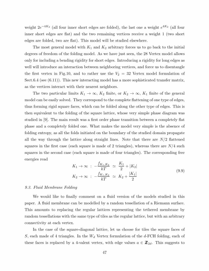
weight 2e−4K2 (all four inner short edges are folded), the last one a weight e4K2 (all four

inner short edges are flat) and the two remaining vertices receive a weight 1 (two short

edges are folded, two are flat). This model will be studied elsewhere.

The most general model with K1 and K2 arbitrary forces us to go back to the initial

degrees of freedom of the folding model. As we have just seen, the 28 Vertex model allows

only for including a bending rigidity for short edges. Introducing a rigidity for long edges as

well will introduce an interaction between neighboring vertices, and force us to disentangle

the first vertex in Fig.10, and to rather use the V2 = 32 Vertex model formulation of

Sect.6.4 (see (6.11)). This new interacting model has a more sophisticated transfer matrix,

as the vertices interact with their nearest neighbors.

The two particular limits K1 → ∞, K2 finite, or K2 → ∞, K1 finite of the general

model can be easily solved. They correspond to the complete flattening of one type of edges,

thus forming rigid square faces, which can be folded along the other type of edges. This is

then equivalent to the folding of the square lattice, whose very simple phase diagram was

studied in [9]. The main result was a first order phase transition between a completely flat

phase and a completely folded one. What makes the model very simple is the absence of

folding entropy, as all the folds initiated on the boundary of the studied domain propagate

all the way through the lattice along straight lines. Note that there are N/2 flattened

squares in the first case (each square is made of 2 triangles), whereas there are N/4 such

squares in the second case (each square is made of four triangles). The corresponding free

energies read

K1 → ∞ : −fK1,K2

kT≃ K1

2+ |K2|

K2 → ∞ : −fK1,K2

kT≃ K2 +

|K1|2

(9.9)

9.3. Fluid Membrane Folding

We would like to finally comment on a fluid version of the models studied in this

paper. A fluid membrane can be modelled by a random tessellation of a Riemann surface.

This amounts to replacing the regular lattices representing the tethered membrane by

random tessellations with the same type of tiles as the regular lattice, but with an arbitrary

connectivity at each vertex.

In the case of the square-diagonal lattice, let us choose for tiles the square faces of

S, each made of 4 triangles. In the Wd Vertex formulation of the d-FCH folding, each of

these faces is replaced by a 4-valent vertex, with edge values a ∈ ZZ2d. This suggests to

47

introduce a fluid version thereof, in which the lattice is replaced by φ4 (4-valent) graphs,

with edge variables a ∈ ZZ2d. A simple way of representing the partition function of such

a model is to consider a Hermitian multi-matrix integral

Z(N, g) =

∫

dM0...dM2d−1e−N Tr(V (M0,...,M2d−1)) (9.10)

where M0, M2, ...,M2d−1 are N×N Hermitian matrices, integrated wrt the standard Haar

measure, and

V (M0, ...,M2d−1) =

2d−1∑

i=0

(1

2gM2

i +d− 1

2M4

i )

+1

4

∑

0≤i6=j≤d−1

(M2i M

2j + 2M2

i+dM2j +M2

i+dM2j+d + 4MiMjMi+dMj+d)

(9.11)

where the quartic terms reproduce the vertices of Fig.18. Moreover, the measure of inte-

gration is normalized so that limg→0 Z(N, g) = 1. The perturbative expansion of LogZ as

a power series of g and N reads LogZ =∑

h,n≥0 N2−2hgnZn,h, where Zn,h is the partition

function for the Wd Vertex model on the set of connected tessellations of surfaces of genus

h with n squares. Unfortunately, even for d = 2 the solution of the model (9.10) is not

known.

Acknowledgements

We thank K. Hallowell for interesting discussions. This work was partially supported

by NSF grant PHY-9722060.

48

References

[1] Y. Kantor and D.R. Nelson, Crumpling Transition in Polymerized Membranes, Phys.

Rev. Lett. 58 (1987) 2774 and Phase Transitions in Flexible Polymeric Surfaces, Phys.

Rev. A 36 (1987) 4020.

[2] D.R. Nelson and L. Peliti, Fluctuations in Membranes with Crystalline and Hexatic

Order, J. Physique 48 (1987) 1085.

[3] M. Paczuski, M. Kardar and D.R. Nelson, Landau Theory of the Crumpling Transition,

Phys. Rev. Lett. 60 (1988) 2638.

[4] F. David and E. Guitter, Crumpling Transition in Elastic Membranes: Renormaliza-

tion Group Treatment, Europhys. Lett. 5 (1988) 709.

[5] M. Baig, D. Espriu and J. Wheater, Phase Transitions in Random Surfaces, Nucl.

Phys. B314 (1989) 587; R. Renken and J. Kogut, Scaling Behavior at the Crumpling

Transition, Nucl. Phys. B342 (1990) 753; R. Harnish and J. Wheater, The Crumpling

Transition of Crystalline Random Surfaces, Nucl. Phys. B350 (1991) 861; J. Wheater

and P. Stephenson, On the Crumpling Transition in Crystalline Random Surfaces,

Phys. Lett. B302 (1993) 447.

[6] P. Di Francesco, O. Golinelli and E. Guitter, Meander, Folding and Arch Configura-

tions, Mathl. Comput. Modelling, Vol. 26, No.8-10 (1997) 97-147, Meanders and the

Temperley-Lieb Algebra, Commun. Math. Phys. 186 (1997), 1-59 and Meanders: a

direct enumeration approach, Nucl. Phys. B482[FS] (1996), 497-535; P. Di Francesco,

Meander Determinants, to appear in Commun. Math. Phys. (1998)

[7] Y. Kantor and M.V. Jaric, Europhys. Lett. 11 (1990) 157.

[8] P. Di Francesco and E. Guitter Entropy of Folding of the Triangular Lattice, Europhys.

Lett. 26 (1994) 455.

[9] P. Di Francesco and E. Guitter Folding Transition of the Triangular Lattice, Phys.

Rev. E50 (1994) 4418-4426.

[10] M. Bowick, P. Di Francesco, O. Golinelli and E. Guitter 3D Folding of the triangular

lattice, Nucl. Phys. B450[FS] (1995) 463-494.

[11] H. Temperley and E. Lieb, Relations between the Percolation and Coloring Problems

and other Graph-Theoretical Problems associated with regular Planar Lattices: Some

Exact Results for the Percolation Problem, Proc. Roy. Soc. A322 (1971) 251-280;

see also the book by P. Martin, Potts Models and Related Problems in Statistical

Mechanics, World Scientific, Singapore (1991) for a review.

[12] R.J. Baxter, Exactly Solved Models in Statistical Mechanics, Academic Press, London

(1982).

[13] P. Di Francesco, B. Eynard and E. Guitter, Coloring Random Triangulations, cond-

mat/9711050, to appear in Nucl. Phys. B (1998).

49