Embed Size (px)
Citation preview
V,
FOCUSED SIMULATED ANNEALING SEARCH: AN APPLICATION TO
JOB-SHOP SCHEDULING *
Norman M. Sadeh and Yoichiro Nakakuki t CMU-RI-TR-94-29
The Robotics Institute Carnegie Mellon University Pittsburgh, PA 15213-3891
September 1994
This do-. *,,. •-.' distribu'
19941227 093 "This research was supported, in part, by the Advanced Research Projects Agency under contract
F30602-91-C-0016 and, in part, by an industrial grant from NEC. tThis research was carried out while the second author was a visiting scientist at Carnegie Mel-
Ion's Robotics Institute. His current address is: NEC C&C Research Laboratories, 4-1-1 Miyazaki, Miyamae-ku, Kawasaki 216, JAPAN.
Abstract
This paper presents a simulated annealing search procedure developed to solve job shop scheduling problems simultaneously subject to tardiness and in- ventory costs. The procedure is shown to significantly increase schedule quality compared to multiple combinations of dispatch rules and release policies, though at the expense of intense computational efforts. A meta-heuristic procedure is developed that aims at increasing the efficiency of simulated annealing by dy- namically inflating the costs associated with major inefficiencies in the current solution. Three different variations of this procedure are considered. One of these variations is shown to yield significant reductions in computation time, es- pecially on problems where search is more likely to get trapped in local minima. We analyze why this variation of the meta-heuristic is more effective than the
others.
i
M
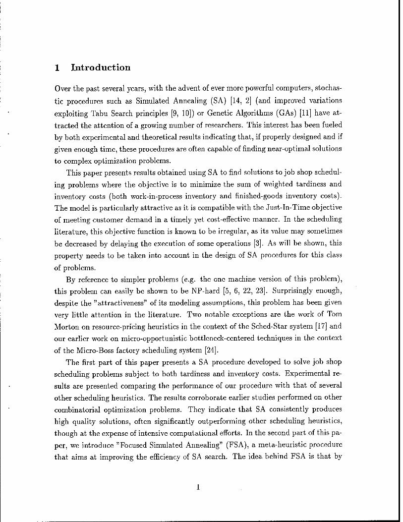
1 Introduction
Over the past several years, with the advent of ever more powerful computers, stochas-
tic procedures such as Simulated Annealing (SA) [14, 2] (and improved variations
exploiting Tabu Search principles [9, 10]) or Genetic Algorithms (GAs) [11] have at-
tracted the attention of a growing number of researchers. This interest has been fueled
by both experimental and theoretical results indicating that, if properly designed and if
given enough time, these procedures are often capable of finding near-optimal solutions
to complex optimization problems.
This paper presents results obtained using SA to find solutions to job shop schedul-
ing problems where the objective is to minimize the sum of weighted tardiness and
inventory costs (both work-in-process inventory and finished-goods inventory costs).
The model is particularly attractive as it is compatible with the Just-In-Time objective
of meeting customer demand in a timely yet cost-effective manner. In the scheduling
literature, this objective function is known to be irregular, as its value may sometimes
be decreased by delaying the execution of some operations [3]. As will be shown, this
property needs to be taken into account in the design of SA procedures for this class
of problems.
By reference to simpler problems (e.g. the one machine version of this problem),
this problem can easily be shown to be NP-hard [5, 6, 22, 23]. Surprisingly enough,
despite the "attractiveness" of its modeling assumptions, this problem has been given
very little attention in the literature. Two notable exceptions are the work of Tom
Morton on resource-pricing heuristics in the context of the Sched-Star system [17] and
our earlier work on micro-opportunistic bottleneck-centered techniques in the context
of the Micro-Boss factory scheduling system [24].
The first part of this paper presents a SA procedure developed to solve job shop
scheduling problems subject to both tardiness and inventory costs. Experimental re-
sults are presented comparing the performance of our procedure with that of several
other scheduling heuristics. The results corroborate earlier studies performed on other
combinatorial optimization problems. They indicate that SA consistently produces
high quality solutions, often significantly outperforming other scheduling heuristics,
though at the expense of intensive computational efforts. In the second part of this pa-
per, we introduce "Focused Simulated Annealing" (FSA), a meta-heuristic procedure
that aims at improving the efficiency of SA search. The idea behind FSA is that by
dynamically inflating the costs associated with major inefficiencies in the existing so-
lution, it is possible to focus the procedure and force it to get rid of these inefficiencies.
By iteratively inflating costs in different subproblems, FSA can reduce the chances that
the procedure gets trapped in local minima. Three variations of this meta-heuristic are
considered that differ in the type of subproblems they rely on: job subproblems, re-
source subproblems, or operation subproblems. Experimental results comparing these
three variations of the meta-heuristic against the original SA procedure show that the
job-based meta-heuristic significantly improves performance, especially on problems
where search is particularly likely to get caught in local minima. We further analyze
why this variation of the meta-heuristic is more effective than the others, trying to
shed some light on why, in general, some decompositions are likely to work better than
others for a given SA procedure.
The balance of this paper is organized as follows. Section 2 provides a formal defi-
nition of the job shop scheduling problem considered in this study. Section 3 presents a
SA search procedure developed for this problem. Section 4 reports experimental results
comparing the performance of the procedure against that of other scheduling heuris-
tics. The concept of Focused Simulated Annealing is introduced in Section 5 and three
variations of this meta-heuristic procedure are developed for the job shop scheduling
problem with tardiness and inventory costs. Performance of these meta-heuristics is
reported in Section 6. These results are further discussed and analyzed in Section 7.
Section 8 presents some concluding remarks.
2 The Job Shop Scheduling Problem with Tardiness and In- ventory Costs
We consider a factory, in which a finite set of jobs, J = {J1J2, ••• ,jn}, has to be
scheduled on a finite set of resources, RES = {Rlf R2, ■ ■ ■, Rm). The jobs are assumed
to be known ahead of time and all resources are assumed to be available over the entire
scheduling horizon. Each job ji requires performing a set of manufacturing operations
Ol = {0[,Ol2,---O
lnt} and, ideally, should be completed by a specific due date, dd\,
for delivery to a customer. Precedence constraints specify a complete order in which
operations in each job have to be performed. By convention, we assume that operation
0\ has to be completed before operation 0\+1 can start (i = 1,2, • • •, n\ - 1).
Each job ji has an earliest acceptable release date, erdh before which it cannot start,
e.g. because the raw materials or components required by this job cannot be delivered
before that date. Each job also has a latest acceptable completion date (or deadline),
lcdh by which it should absolutely be completed, e.g. because the customer would
otherwise refuse delivery of the order. For each job, we assume that erdi < ddi < lcd\.
Furthermore, we assume that these constraints are loose enough to always allow for
the construction of a feasible schedule (i.e. we are not concerned with the detection of
infeasible problems).
This paper considers problems in which each operation 0\ requires a single resource
R[ € RES and the order in which a job visits different resources varies from one
job to another. Each resource can only process one operation at a time and is non-
preemptable. The duration du\ of each operation 0\ is assumed to be known.
The problem requires finding a schedule (i.e. a set of start times, st\, for all op-
erations, 0\) that satisfies all these constraints while minimizing the sum of tardiness
costs and inventory costs of all the jobs.
Specifically, each job ji incurs a positive marginal tardiness cost tardi for each
unit of time that it finishes past its due date ddi. Marginal tardiness costs generally
correspond to tardiness penalties, interests on lost profits, loss of customer goodwill,
etc. The total tardiness cost of job jh in a given schedule, is measured as: TARD =
tardi • MAX(0, C\ - ddi) where C\ is the completion date of job jt. That is Ci =
stlni + dulni, where 0l
ni is the last operation of j\.
Inventory costs on the other hand can be introduced at the level of any operation
in a job. In our model, each operation 0\ can have its own non-negative marginal
inventory cost, in\. This is the marginal cost that is incurred for each unit of time
that spans between the start time of this operation and either the completion date of
the job or its due date, whichever is larger. In other words, the total inventory cost
introduced by an operation 0\ in a given schedule is:
INVf = in\ ■ (MAX(Chdd,) - st1^
Typically, the first operation in a job introduces marginal inventory costs that corre-
spond to interests on the costs of raw materials, interests on processing costs (for that
first operation), and marginal holding costs. Following operations introduce additional
inventory costs such as interests on processing costs, interests on the costs of additional
raw materials or components required by these operations, etc. Additional details on
this model can be found in [23, 24].
The total cost of a schedule is: ni
For reasons that will become clearer in Section 5, it is often useful to look at the
total tardiness and inventory costs of a job as sums of tardiness and inventory costs
introduced by each of the operations in the job. For each operation O], we can define
a best start time (or "just-in-time" start time), bst\, where:
, _ J ddi- du\ {% = ni) bSti ~ \ bsti+1 - du\ (1 < « < ni)
Accordingly, the tardiness cost TARD1 of job jt in a given schedule, can be rewritten
as. JJJ
TARD1 = £ tcost\
where,
tcost1; { tardi ■ MAX(0, st\ - bst\) (* = 1)
tardi • {MAX{0, st't - 6s*{) - MAX(0, st1^ - bst1^)} (1< i < n,) iardx ■ {MAX(0, Ci - ddi) - MAX(0, st1^ - bst1^)} (i = nt)
tcost'i can be seen as the contribution of operation 0\ to the total tardiness cost of job
31. Similarly, the total inventory cost of a job ji can be rewritten as:
ni
INV1 = Y,icost\ t=l
where:
rm,i ■ 4 S invl-iMAXistl + du^dd^-st'i) (i = n,) INVl = zcost, = | .nvi. {sA+i _ at|) (1 < { < ni)
and inv\ = ELi "**• Accordingly, the total cost of a schedule can also be expressed
as: ni
£ TARD1 + £ INV1 = E E (<cost\ + icostli) lej ieJ ieJ «=i
For the sake of simplicity, the remainder of this paper further assumes that time
is discrete, i.e. that job due dates/earliest acceptable release dates/latest acceptable
completion dates and operation durations can only can only take integer values.
The following section introduces a SA procedure developed for this problem.
3 A Simulated Annealing Procedure
Simulated Annealing (SA) is a general-purpose search procedure that generalizes iter-
ative improvement approaches to combinatorial optimization by sometimes accepting
transitions to lower quality solutions so as to avoid getting trapped in local minima
[14, 2]. SA procedures have been successfully applied to a variety of combinatorial op-
timization problems, including Traveling Salesman Problems [2], Graph Partitioning
Problems [12], Graph Coloring Problems [13], Vehicle Routing Problems [21], Design
of Integrated Circuits, Minimum Makespan Flow-Shop Scheduling Problems [20], Min-
imum Makespan Job Shop Scheduling Problems [16, 26], etc.
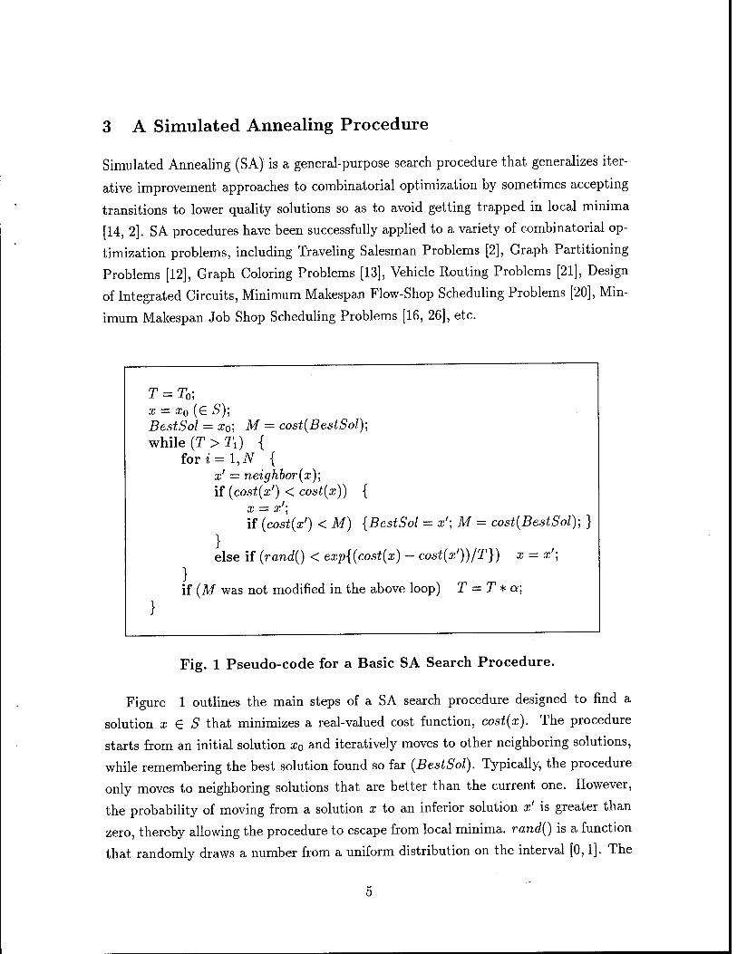
T = T0; x = x0 (e S); BestSol = x0; M = cost(BestSol); while (T>T1) {
fori = l,N { x' = neighbor(x); if (cost(x') < cost(x)) {
if (cost(x') < M) {BestSol = x'; M = cost(BestSol); }
else if (randQ < exp{(cost(x) - cost(x'))/T}) x = x';
if (M was not modified in the above loop) T = T * a;
Fig. 1 Pseudo-code for a Basic SA Search Procedure.
Figure 1 outlines the main steps of a SA search procedure designed to find a
solution x e S that minimizes a real-valued cost function, cost(x). The procedure
starts from an initial solution x0 and iteratively moves to other neighboring solutions,
while remembering the best solution found so far (BestSol). Typically, the procedure
only moves to neighboring solutions that are better than the current one. However,
the probability of moving from a solution x to an inferior solution x' is greater than
zero, thereby allowing the procedure to escape from local minima. randQ is a function
that randomly draws a number from a uniform distribution on the interval [0,1]. The
so-called temperature, T, of the procedure is a parameter controlling the probability of
accepting a transition to a lower quality solution. It is initially set to a high value, T0,
thereby frequently allowing such transitions. If, after N iterations, the best solution
found by the procedure has not improved, the temperature parameter T is decremented
by a factor a (0 < a < 1). When the temperature drops below a preset level, 2\, the
procedure stops and the best solution it found (BestSol) is returned (not shown in the
pseudo-code in Figure 1).
As indicated earlier, procedures similar to the one outlined above have been suc-
cessfully applied to other scheduling problems such as the minimum makespan job-shop
scheduling problem 1. When dealing with regular scheduling objectives such as min-
imum makespan, it is possible to limit search to permutations of operations on the
same machine. For instance, in their SA procedure, Van Laarhoven et al. exploit this
observation and restrict the neighborhood structure to permutations of consecutive
operations on a same machine [26]. In the case of scheduling problems with irregular
objectives, such a neighborhood structure would not be sufficient, as it does not allow
for the insertion of idle-time in the schedule, which sometimes improves the quality of
a solution 2. Here, two main approaches can be considered. A first approach would
be to combine a SA procedure relying on permutation-based neighborhoods with a
procedure that inserts idle-time optimally. As it turns out, the problem of inserting
idle time optimally in a schedule, given completely specified sequences of operations on
each machine, can be formulated as a Linear Programming (LP) problem and, hence,
can be solved in polynomial time (See Appendix A for details). When considering
the permutation of two operations, the SA procedure would first invoke an idle-time
insertion procedure to compute the cost of the best schedule compatible with the new
set of sequencing decisions. Based on this cost and the cost of the current solution,
the search procedure would probabilistically determine whether or not to accept the
transition. Nevertheless, at the present time, the idle time insertion procedures that
the authors are aware of for the job shop scheduling problem remain too slow and
!The makespan of a schedule is the length of the time interval that spans between the start time of the first released job and the end time of the last completed job.
Scheduling problems with regular objective functions have been shown to be reducible to sequenc- ing problems [1]. Given fixed operation sequences on each machine, the schedule obtained by starting each operation as early as possible is undominated. With irregular objectives, this is no longer the case and it is sometimes better to delay the start of some operations. Here, we generically refer to the problem of deciding by how much to delay operations as the problem of "inserting idle time" in
the schedule.
would significantly limit the number of solutions that SA could explore in a reasonable
amount of time 3.
Instead, an alternative neighborhood structure was adopted that directly allows
for idle time insertion. This structure, which is described below, lends itself to quick
updates of the cost function. A possibly more subjective advantage has to do with the
fact that the resulting procedure relies solely on SA and hence is not affected by the
performance of a separate idle time insertion procedure. Specifically, the neighborhood
function used in our implementation randomly selects among three types of modifica-
tion operators, respectively referred to below as "RIGHT-SHIFT", "LEFT-SHIFT"
and "EXCHANGE":
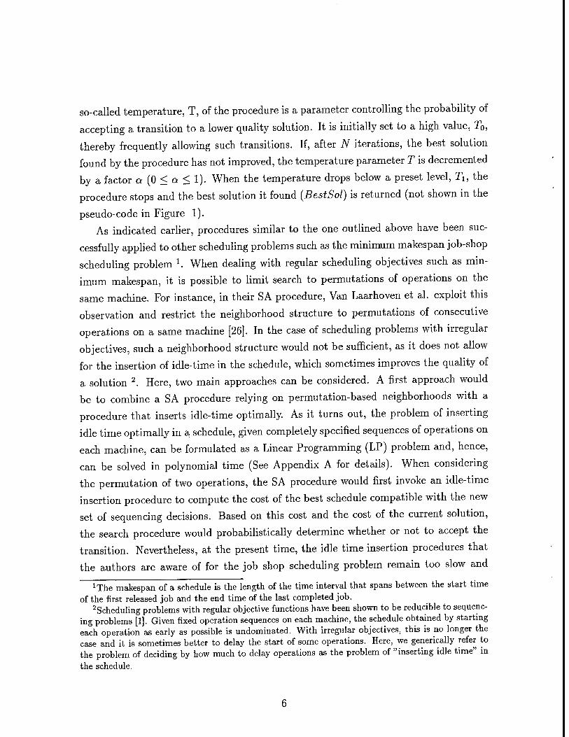
RIGHT-SHIFT This operator randomly chooses a "right-shiftable" operation and
increases its start time by one time unit (Figure 2-(a)). An operation is assumed to be
"right-shiftable", if it can be shifted by one time unit without bumping into another
operation on the same resource or violating the latest acceptable completion date of
the job to which it belongs (Figure 2-(b)). Precedence constraints within a job are
ignored when determining whether or not an operation can be right-shifted. Instead,
as will be seen later, these constraint violations are taken care of by inserting artificial
costs in the objective function.
Resource R Resource R
or
Resource R
t+1
(a) SHIFT-RIGHT
Resource R
led,
(b) not shiftable
Fig. 2 RIGHT-SHIFT operator 3For instance, using the CPLEX Linear Programming package on a DECstation 5000/200, inserting
idle time optimally in a 100 operation job shop schedule takes about 1 CPU second. Taking into account similarities between the current schedule and the schedule obtained after permuting the order of two operations on the same resource, it is generally possible to reduce the time required to re- optimize the schedule to about 0.1 to 0.2 CPU seconds. Even under these conditions, a SA run of about 10 minutes would only be able to explore a few thousand solutions.
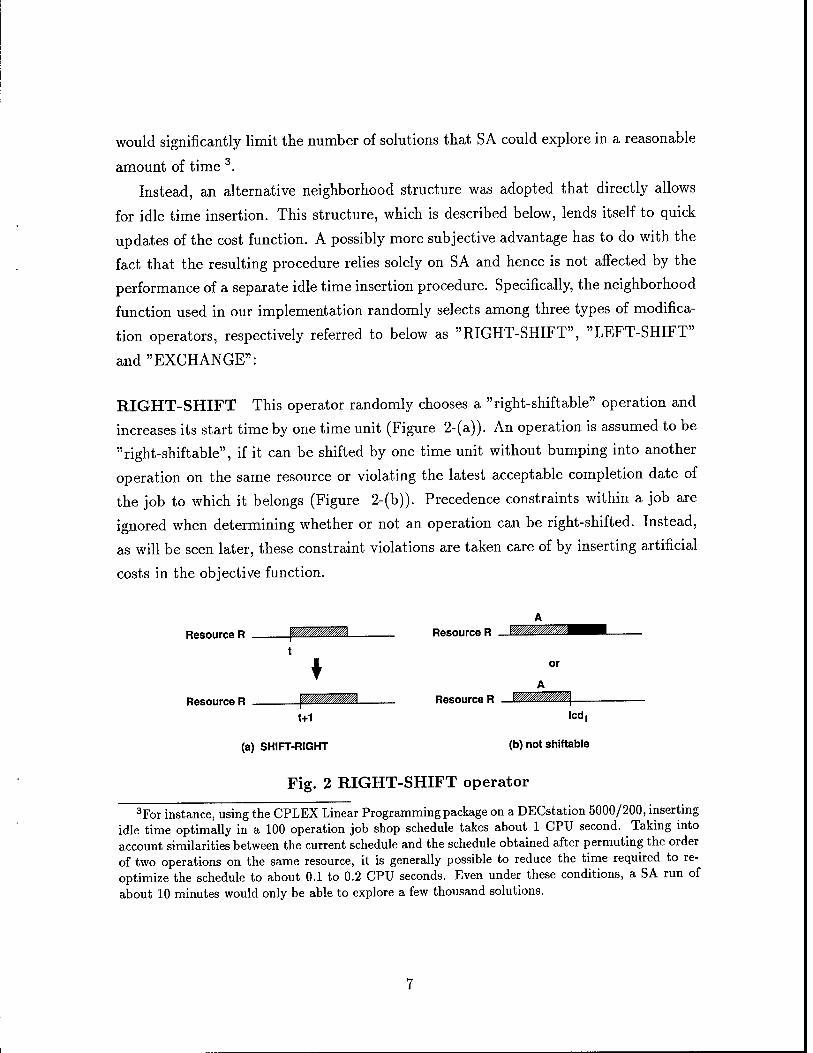
LEFT-SHIFT This operator is the mirror image of RIGHT-SHIFT. It randomly
picks a "left-shiftable" operation and decreases its start time by one time unit (Figure
3-(a)). It is assumed that an operation cannot be shifted left, if it would either bump
into an adjacent operation on the same resource (top case in Figure 3-(b)) or violate
the earliest acceptable release date of the job to which it belongs (bottom case in Figure
3-(b)).
Resource R Resource R
or
Resource R Resource R
t-1
(a) SHIFT-LEFT
erd,
(b) not shiftable
Fig. 3 LEFT-SHIFT operator
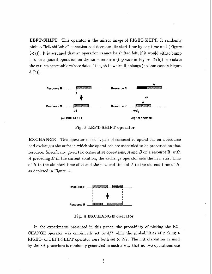
EXCHANGE This operator selects a pair of consecutive operations on a resource
and exchanges the order in which the operations are scheduled to be processed on that
resource. Specifically, given two consecutive operations, A and B on a resource R, with
A preceding B in the current solution, the exchange operator sets the new start time
of B to the old start time of A and the new end time of A to the old end time of B,
as depicted in Figure 4.
Resource R
Resource R
♦
Fig. 4 EXCHANGE operator
In the experiments presented in this paper, the probability of picking the EX-
CHANGE operator was empirically set to 3/7 while the probabilities of picking a
RIGHT- or LEFT-SHIFT operator were both set to 2/7. The initial solution x0 used
by the SA procedure is randomly generated in such a way that no two operations use
the same resource at the same time. As with the RIGHT- and LEFT-SHIFT opera-
tor, precedence constraints between consecutive operations within a same job are not
enforced in the process. Instead these constraints are enforced using artificial costs. If
an operation 0\ overlaps with a preceding operation 0\_x (within the same job _;'/), an
artificial cost fcost\ is introduced in the objective function:
ni
cost(x) = 5ZX1 (/cos*! + tcost'i + icost'i)
where fcosti is proportional to the amount of overlap between 0\ and its predecessor
0\_v Specifically:
fcost[ = 0
fcost\ = ß ■ roas(M*'-i + du\-\ ~ st\) (* > 2)
where ß is a large positive constant.
The next section summarizes the results of experiments comparing this basic SA
procedure with several other scheduling heuristics.
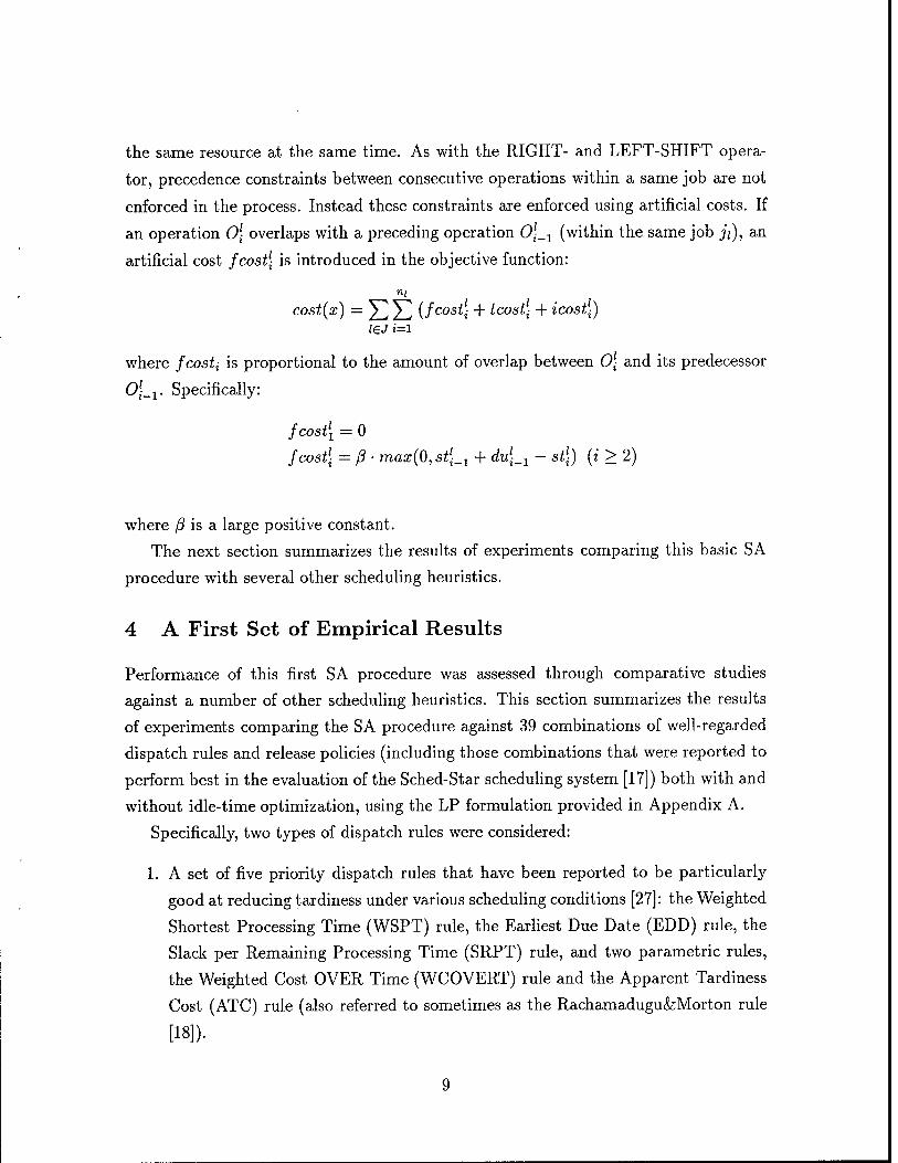
4 A First Set of Empirical Results
Performance of this first SA procedure was assessed through comparative studies
against a number of other scheduling heuristics. This section summarizes the results
of experiments comparing the SA procedure against 39 combinations of well-regarded
dispatch rules and release policies (including those combinations that were reported to
perform best in the evaluation of the Sched-Star scheduling system [17]) both with and
without idle-time optimization, using the LP formulation provided in Appendix A.
Specifically, two types of dispatch rules were considered:
1. A set of five priority dispatch rules that have been reported to be particularly
good at reducing tardiness under various scheduling conditions [27]: the Weighted
Shortest Processing Time (WSPT) rule, the Earliest Due Date (EDD) rule, the
Slack per Remaining Processing Time (SRPT) rule, and two parametric rules,
the Weighted Cost OVER Time (WCOVERT) rule and the Apparent Tardiness
Cost (ATC) rule (also referred to sometimes as the Rachamadugu&Morton rule
[18]).
2. An exponential version of the parametric early/tardy dispatch rule recently de-
veloped by Ow and Morton [22, 17] and referred to below as EXP-ET. This rule
differs from the other 5 in that it can explicitly account for both tardiness and
inventory costs.
EXP-ET was successively run in combination with two release policies: an intrinsic
release policy that only releases jobs when their priorities become positive, as sug-
gested in [17], and an immediate release policy (IM-REL) that allowed each job to
be relased immediately. The other five dispatch rules were also successively run in
combination with two release policies: an immediate release policy and the Average
Queue Time release policy (AQT) described in [17]. AQT is a parametric release policy
that estimates queuing time as a multiple of the average job duration (the look-ahead
parameter serving as the multiple). A job's release date is determined by offsetting the
due date of the job by the sum of its total duration and its estimated queuing time.
In their evaluation of the SCHED-STAR scheduling system, Morton et al. report that
the combination of WCOVERT and AQT performed best after their SCHED-STAR
system and was within 0.1% of the best schedule in 42% of the problems they studied
and within 4% in 70% of their problems [17]. They also report that the next best
scheduling heuristic is EXP-ET in combination with its intrinsic release policy.
Combinations of release policies and dispatch rules with a look-ahead parameter
were successively run with four different parameter values that had been identified as
producing the best results. By combining these different dispatch rules, release policies
and parameter settings a total of 39 heuristics4 was obtained.
These 39 combinations of priority dispatch rules and release policies were run in
two different ways:
1. On each problem, the best of the 39 schedules produced by these combinations
was recorded. In this case, out of the 39 combinations, 13 performed best on
at least one of the 40 problems considered in the study. These 13 combinations
included 5 of the 6 dispatch rules (SRPT was never best on this set of problems)
and all 3 release policies.
4The 39 combinations were as follows: EXP-ET and its intrinsic policy (times four parameter settings), EXP-ET/IM-REL (times four parameter settings), EDD/AQT (times four parameter set- tings), EDD/IM-REL, WSPT/AQT (times four parameter settings), WSPT/IM-REL, SRPT/AQT (times four parameter settings), SRPT/IM-REL, WCOVERT/IM-REL (times four parameter set- tings), WCOVERT/AQT (times four parameter settings), ATC/IM-REL (times four parameter set- tings), ATC/AQT (times four parameter settings).
10
2. On each problem, each of the 39 schedules obtained by these combinations was
post-processed using an LP program to insert idle time optimally. Again, on each
problem, the best of the 39 post-processed schedules was recorded for comparison
against the SA procedure. In this case, out of the 39 combinations, 11 performed
best (after post-processing) on at least one of the 40 problems considered in the
study. These 11 combinations included 5 of the 6 dispatch rules (here, WSPT
was never best) and all 3 release policies.
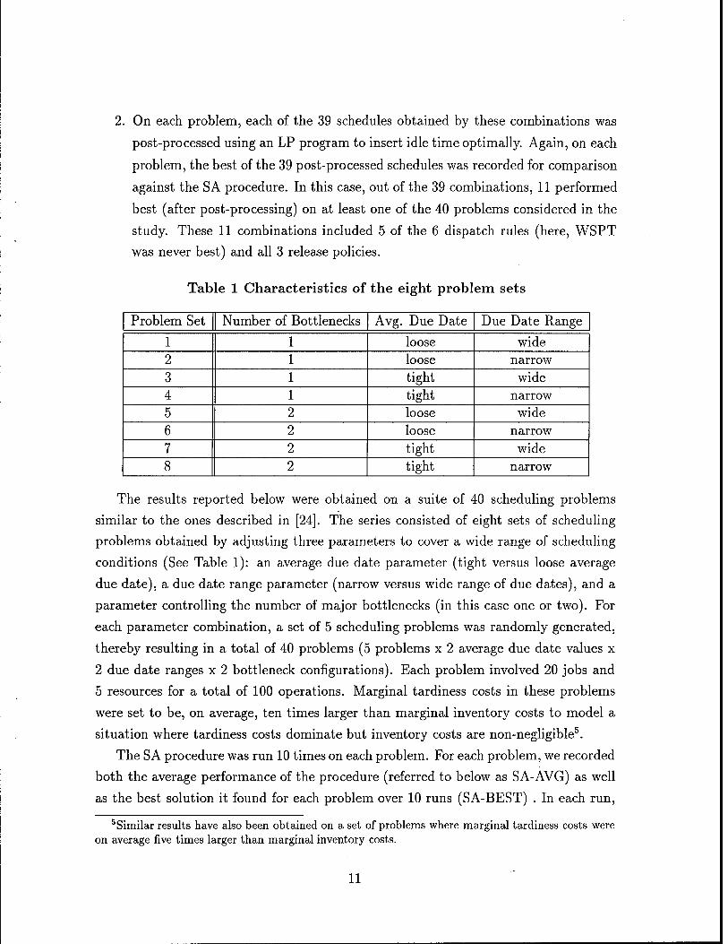
Table 1 Characteristics of the eight problem sets
Problem Set Number of Bottlenecks Avg. Due Date Due Date Range
1 1 loose wide 2 1 loose narrow 3 1 tight wide 4 1 tight narrow 5 2 loose wide 6 2 loose narrow 7 2 tight wide 8 2 tight narrow
The results reported below were obtained on a suite of 40 scheduling problems
similar to the ones described in [24]. The series consisted of eight sets of scheduling
problems obtained by adjusting three parameters to cover a wide range of scheduling
conditions (See Table 1): an average due date parameter (tight versus loose average
due date), a due date range parameter (narrow versus wide range of due dates), and a
parameter controlling the number of major bottlenecks (in this case one or two). For
each parameter combination, a set of 5 scheduling problems was randomly generated,
thereby resulting in a total of 40 problems (5 problems x 2 average due date values x
2 due date ranges x 2 bottleneck configurations). Each problem involved 20 jobs and
5 resources for a total of 100 operations. Marginal tardiness costs in these problems
were set to be, on average, ten times larger than marginal inventory costs to model a
situation where tardiness costs dominate but inventory costs are non-negligible5.
The SA procedure was run 10 times on each problem. For each problem, we recorded
both the average performance of the procedure (referred to below as SA-AVG) as well
as the best solution it found for each problem over 10 runs (SA-BEST) . In each run,
5Similar results have also been obtained on a set of problems where marginal tardiness costs were on average five times larger than marginal inventory costs.
11
the initial temperature, To, was set to 700, temperature T\ was 6.25 and the cooling
rate a was 0.85. The value of ß was 1000 6. The number N of iterations in the
inner-loop of the procedure (See Figure 1) was set to 300,000.
25000
4 5
Problem Sei
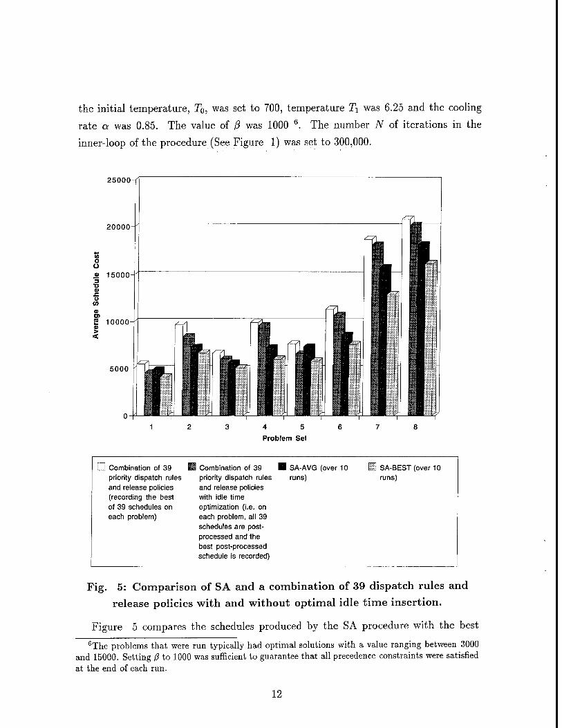
G Combination of 39 ■ Combination of 39 ■ SA-AVG (over 10 D SA-BEST(over10 priority dispatch rules priority dispatch rules runs) runs) and release policies and release policies (recording the best with idle time of 39 schedules on optimization (i.e. on each problem) each problem, all 39
schedules are post- processed and the best post-processed schedule is recorded)
Fig. 5: Comparison of SA and a combination of 39 dispatch rules and
release policies with and without optimal idle time insertion.
Figure 5 compares the schedules produced by the SA procedure with the best 6The problems that were run typically had optimal solutions with a value ranging between 3000
and 15000. Setting ß to 1000 was sufficient to guarantee that all precedence constraints were satisfied at the end of each run.
12
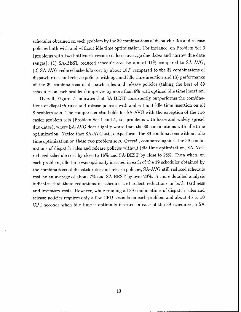
schedules obtained on each problem by the 39 combinations of dispatch rules and release
policies both with and without idle time optimization. For instance, on Problem Set 6
(problems with two bottleneck resources, loose average due dates and narrow due date
ranges), (1) SA-BEST reduced schedule cost by almost 11% compared to SA-AVG,
(2) SA-AVG reduced schedule cost by about 18% compared to the 39 combinations of
dispatch rules and release policies with optimal idle time insertion and (3) performance
of the 39 combinations of dispatch rules and release policies (taking the best of 39
schedules on each problem) improves by more than 6% with optimal idle time insertion.
Overall, Figure 5 indicates that SA-BEST consistently outperforms the combina-
tions of dispatch rules and release policies with and without idle time insertion on all
8 problem sets. The comparison also holds for SA-AVG with the exception of the two
easier problem sets (Problem Set 1 and 5, i.e. problems with loose and widely spread
due dates), where SA-AVG does slightly worse than the 39 combinations with idle time
optimization. Notice that SA-AVG still outperforms the 39 combinations without idle
time optimization on these two problem sets. Overall, compared against the 39 combi-
nations of dispatch rules and release policies without idle time optimization, SA-AVG
reduced schedule cost by close to 16% and SA-BEST by close to 28%. Even when, on
each problem, idle time was optimally inserted in each of the 39 schedules obtained by
the combinations of dispatch rules and release policies, SA-AVG still reduced schedule
cost by an average of about 7% and SA-BEST by over 20%. A more detailed analysis
indicates that these reductions in schedule cost reflect reductions in both tardiness
and inventory costs. However, while running all 39 combinations of dispatch rules and
release policies requires only a few CPU seconds on each problem and about 45 to 50
CPU seconds when idle time is optimally inserted in each of the 39 schedules, a SA
13
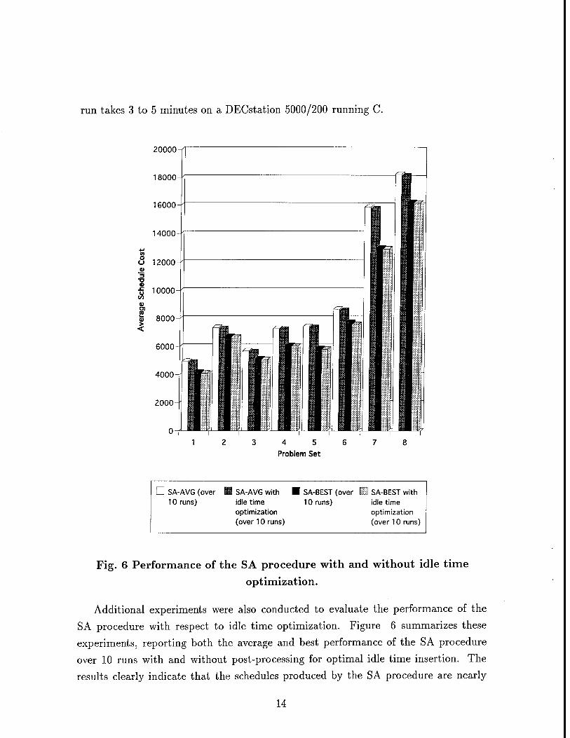
run takes 3 to 5 minutes on a DECstation 5000/200 running C.
20000
18000
16000
D SA-AVG (over 10 runs)
■ SA-AVG with ■ SA-BEST (over 11 SA-BEST with idle time 10 runs) idle time optimization optimization (over 10 runs) (over 10 runs)
Fig. 6 Performance of the SA procedure with and without idle time
optimization.
Additional experiments were also conducted to evaluate the performance of the
SA procedure with respect to idle time optimization. Figure 6 summarizes these
experiments, reporting both the average and best performance of the SA procedure
over 10 runs with and without post-processing for optimal idle time insertion. The
results clearly indicate that the schedules produced by the SA procedure are nearly
14
optimal with respect to idle time insertion, thereby validating the choice of the LEFT-
and RIGHT-SHIFT operators used to define the neighborhood of the procedure. On
average, idle time insertion improved performance of SA-BEST by a meager 0.94%
(with a standard deviation of 0.8%) and that of SA-AVG by 1.02% (with a standard
deviation of 0.5%). The results in Figure 5 and 6 generally attest to the ability of the SA procedure
to produce high quality solutions, often significantly reducing schedule cost compared
to other well-regarded scheduling heuristics. They also indicate that the computa-
tional requirements of the procedure are quite large compared to these other heuristics,
though experiments with larger problems suggest that the average complexity of our
SA procedure only grows linearly with the size of the problem.
Finally, we observe that the performance of the SA procedure can significantly vary
from one run to another, as illustrated by the results in Figure 5. In our experiments,
an average run of SA produced schedules with costs 14% higher than those of the best
schedule obtained over 10 runs (SA-AVG vs. SA-BEST). This suggests that important
speedups could possibly be obtained if the procedure was more consistent in producing
high quality solutions. In the following section, a meta-heuristic procedure is presented
that aims at reducing performance variability using artificial costs to dynamically focus
the SA procedure on critical subproblems.
5 Focused Simulated Annealing Search
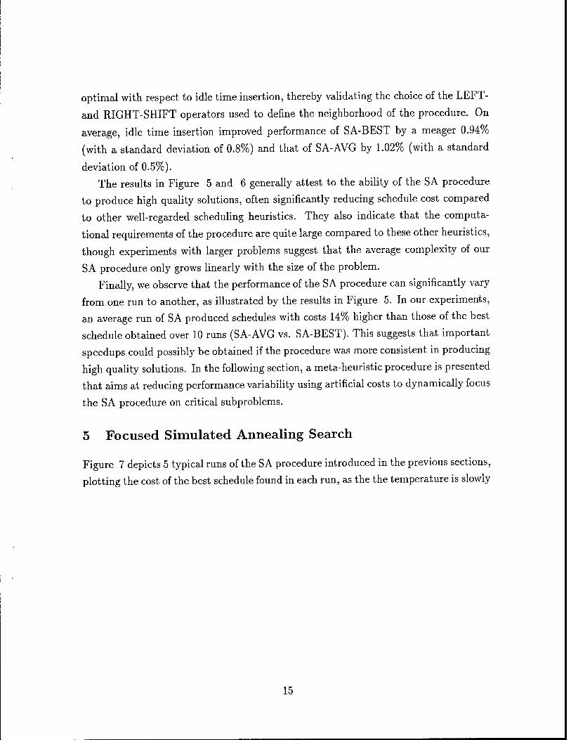
Figure 7 depicts 5 typical runs of the SA procedure introduced in the previous sections,
plotting the cost of the best schedule found in each run, as the the temperature is slowly
15
lowered over time.
Cost i I
25000-
20000-
15000-
200 100 -i—
50 -1—
25 ->-Temp.
12.5 6.25
Fig. 7 Solution improvement in 5 runs of SA.
The behavior exhibited in Figure 7 is characteristic of SA search procedures: the
largest improvements are observed at relatively high temperatures. In the case of
our SA procedure, we observed that below T = 50 the quality of the solution never
improved by more than a few percent. In other words, the early stage of the procedure
is the one that determines whether or not the procedure will get trapped in a local
minimum (e.g. See run A in Figure 7). The remainder of this section describes a
meta-heuristic that relies on the dynamic introduction of artificial costs in the objective
function to focus SA on critical subproblems and attempt to steer clear of local minima
during the high temperature phase of the procedure. Below we refer to the resulting
procedure as "Focused Simulated Annealing" (FSA) search.
To improve the quality of an existing solution, FSA iteratively identifies major
inefficiencies in the current solution and attempts to make these inefficiencies more
obvious to the search procedure by artificially inflating their costs. As a result, the
search procedure works harder on getting rid of these inefficiencies, possibly introducing
new inefficiencies in the process. By regularly tracking sources of inefficiency in the
existing solution and reconfiguring the cost function to eliminate these inefficiencies,
FSA can increase the chances that the procedure finds a high quality solution.
16
T = T0; x = x0 (e S); BestSol = x0; M = cost(BestSol); while (r>Ti) {
if (r > r2) CritSubp = identify-high-cost-subp (x);
else CritSubp = 0;
fori = l,N { x' = neighbor(x); if (costl (x') < costl(x)) x = x'; else if (randQ < exp{(cost 1 (x) - costl (x'))/T}) x = x'; if (cost(x') < M) {BestSol = x'; M = cost(BestSol);}
} if (M was not modified in the above loop) T = T * a;
}
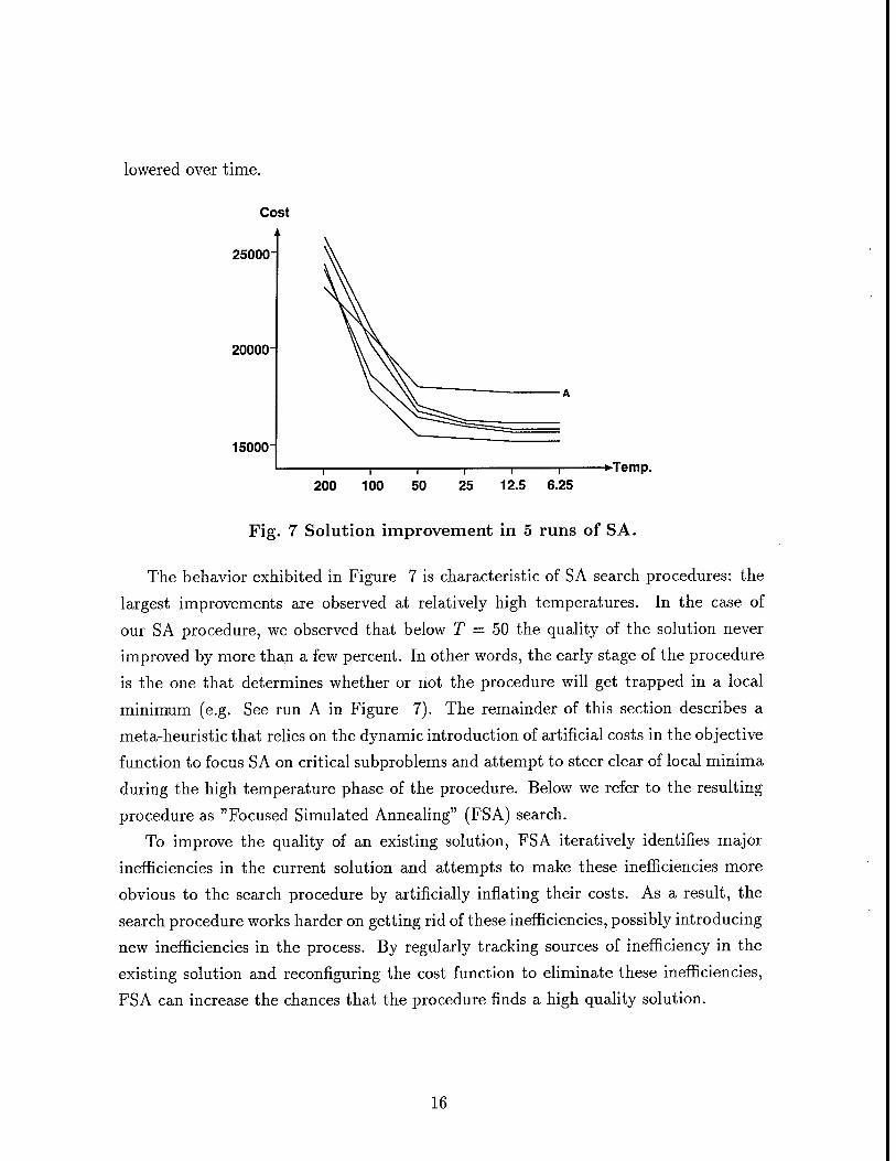
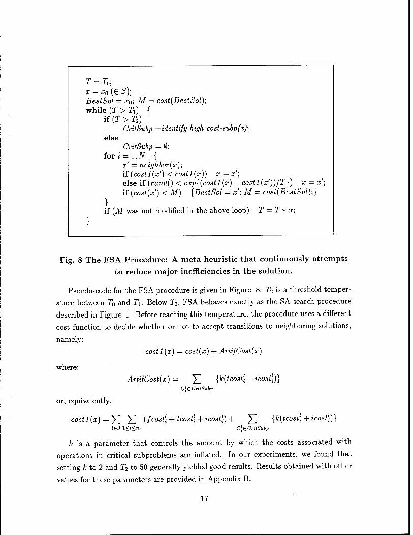
Fig. 8 The FSA Procedure: A meta-heuristic that continuously attempts
to reduce major inefficiencies in the solution.
Pseudo-code for the FSA procedure is given in Figure 8. T2 is a threshold temper-
ature between T0 and 2\. Below T2, FSA behaves exactly as the SA search procedure
described in Figure 1. Before reaching this temperature, the procedure uses a different
cost function to decide whether or not to accept transitions to neighboring solutions,
namely:
costl(x) = cost(x) + ArtifCost(x)
where:
ArtifCost(x) = J2 {k(tcost\ + icost\)} OJG CritSubp
or, equivalently:
costl (x) = Y^ E {fcostli + tcostli + icostb+ £ {k{tcost\ + icost\)} leJl<i<nt OleCritSubp
& is a parameter that controls the amount by which the costs associated with
operations in critical subproblems are inflated. In our experiments, we found that
setting A: to 2 and T2 to 50 generally yielded good results. Results obtained with other
values for these parameters are provided in Appendix B.
17
Notice that inflating the costs associated with one or several subproblems is equiv-
alent to reducing the temperature associated with the corresponding components of
the objective function (or raising the temperature in the remainder of the problem).
Accordingly, FSA can be viewed as a SA procedure in which transition probabilities
are subject to different temperatures in different parts of the problem. Temperatures
in different subproblems are regularly modified (lowered or raised) to get rid of ma-
jor inefficiencies in one part or another of the working solution. In this regard, FSA
is reminiscent of the Strategic Oscillation idea of developing non-monotonic cooling
schedules [7, 21, 10]. However, while Strategic Oscillation cooling schedules proposed
in the literature vary temperature in the entire problem, FSA emphasizes selective
temperature variations in dynamically identified subproblems, as detailed below.
The specific parts of the solution in which FSA attempts to eliminate inefficiencies
are determined by the identify-high-cost-subp() function. Here several variations of
the procedure are considered that differ in the way they decompose the problem: a
job-based variation, a resource-based variation and an operation-based variation.
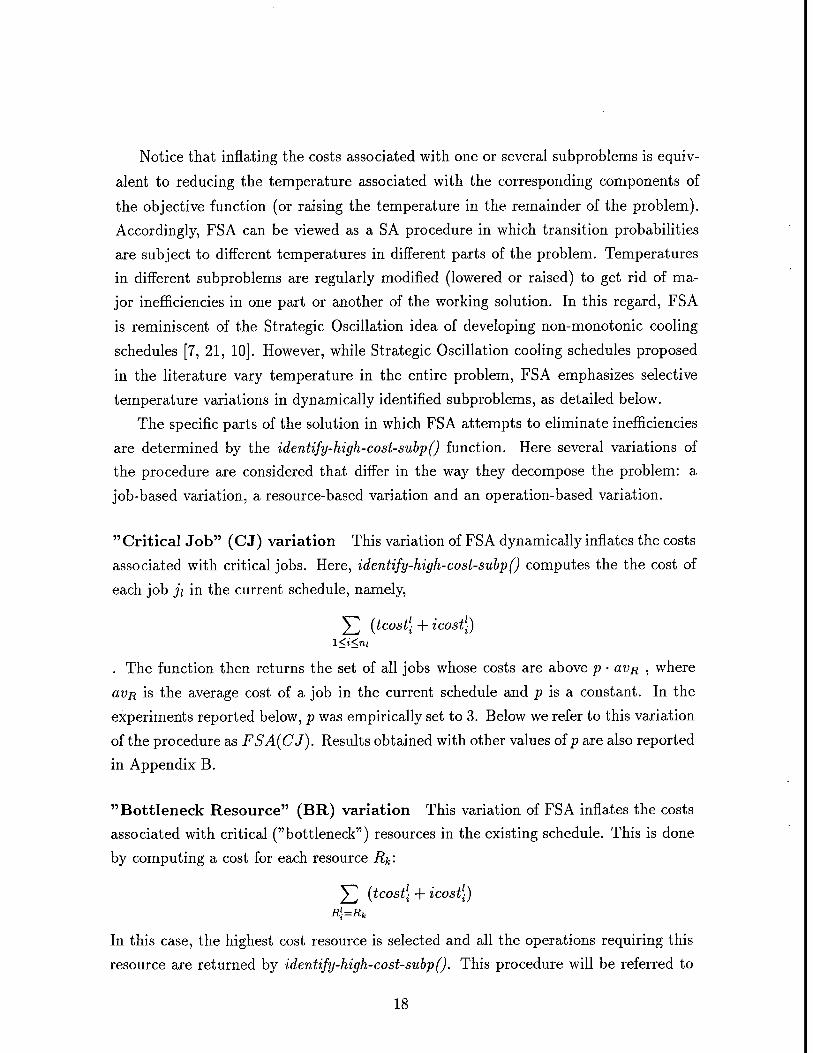
"Critical Job" (CJ) variation This variation of FSA dynamically inflates the costs
associated with critical jobs. Here, identify-high-cost-subp() computes the the cost of
each job ji in the current schedule, namely,
y^ (tcost\ + icostl) l<{<n;
. The function then returns the set of all jobs whose costs are above p • CLVR , where
avn is the average cost of a job in the current schedule and p is a constant. In the
experiments reported below, p was empirically set to 3. Below we refer to this variation
of the procedure as FSA(CJ). Results obtained with other values of p are also reported
in Appendix B.
"Bottleneck Resource" (BR) variation This variation of FSA inflates the costs
associated with critical ("bottleneck") resources in the existing schedule. This is done
by computing a cost for each resource Rk'-
y^ (tcost\ + icost\) R\=Rk
In this case, the highest cost resource is selected and all the operations requiring this
resource are returned by identify-high-cost-subp(). This procedure will be referred to
18
as FSA{BR).
"Critical Operation" (CO) variation Here, FSA focuses on critical operations
rather than critical jobs or critical resources. The average cost of an operation in the
current schedule, avo, is computed:
avo = YL Y, (tcosi\ + icostli)/J2 ni ieji<i<rn leJ
All the operations with a cost above q ■ av0 are considered critical, q is a constant.
In the experiments reported below, q was equal to 3. We will denote this procedure
FSA{CO). Results obtained with other values of q are also reported in Appendix B.
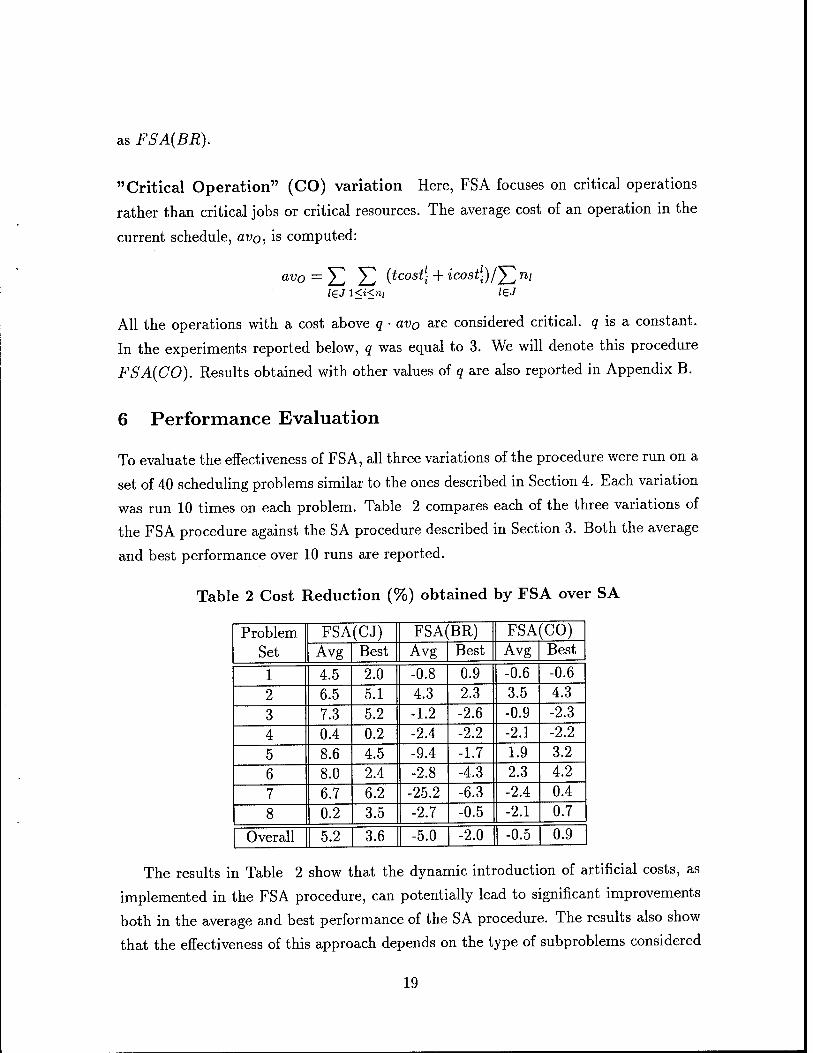
6 Performance Evaluation
To evaluate the effectiveness of FSA, all three variations of the procedure were run on a
set of 40 scheduling problems similar to the ones described in Section 4. Each variation
was run 10 times on each problem. Table 2 compares each of the three variations of
the FSA procedure against the SA procedure described in Section 3. Both the average
and best performance over 10 runs are reported.
Table 2 Cost Reduction (%) obtained by FSA over SA
Problem Set
FSA(CJ) FSA(BR) FSA (CO) Avg Best Avg Best Avg Best
1 4.5 2.0 -0.8 0.9 -0.6 -0.6
2 6.5 5.1 4.3 2.3 3.5 4.3
3 7.3 5.2 -1.2 -2.6 -0.9 -2.3
4 0.4 0.2 -2.4 -2.2 -2.1 -2.2
5 8.6 4.5 -9.4 -1.7 1.9 3.2
6 8.0 2.4 -2.8 -4.3 2.3 4.2
7 6.7 6.2 -25.2 -6.3 -2.4 0.4
8 0.2 3.5 -2.7 -0.5 -2.1 0.7
Overall 5.2 3.6 -5.0 -2.0 -0.5 0.9
The results in Table 2 show that the dynamic introduction of artificial costs, as
implemented in the FSA procedure, can potentially lead to significant improvements
both in the average and best performance of the SA procedure. The results also show
that the effectiveness of this approach depends on the type of subproblems considered
19
by the procedure. While FSA(CJ) reduced schedule cost by an average of 5.2% and
improved the quality of the best schedule found in 10 runs by an average of 3.6%, the
other two variations of the procedure, FSA(BR) and FSA(CO), did not fare as well.
FSA(CO) performed approximately like the original SA procedure and FSA(BR) actu-
ally did worse. Below, we further analyze the performance improvement obtained with
FSA(CJ). In the following section, we attempt to explain why FSA(CO) and FSA(BR)
did not perform as well. For now, we further analyze the performance improvements
observed with FSA(CJ).
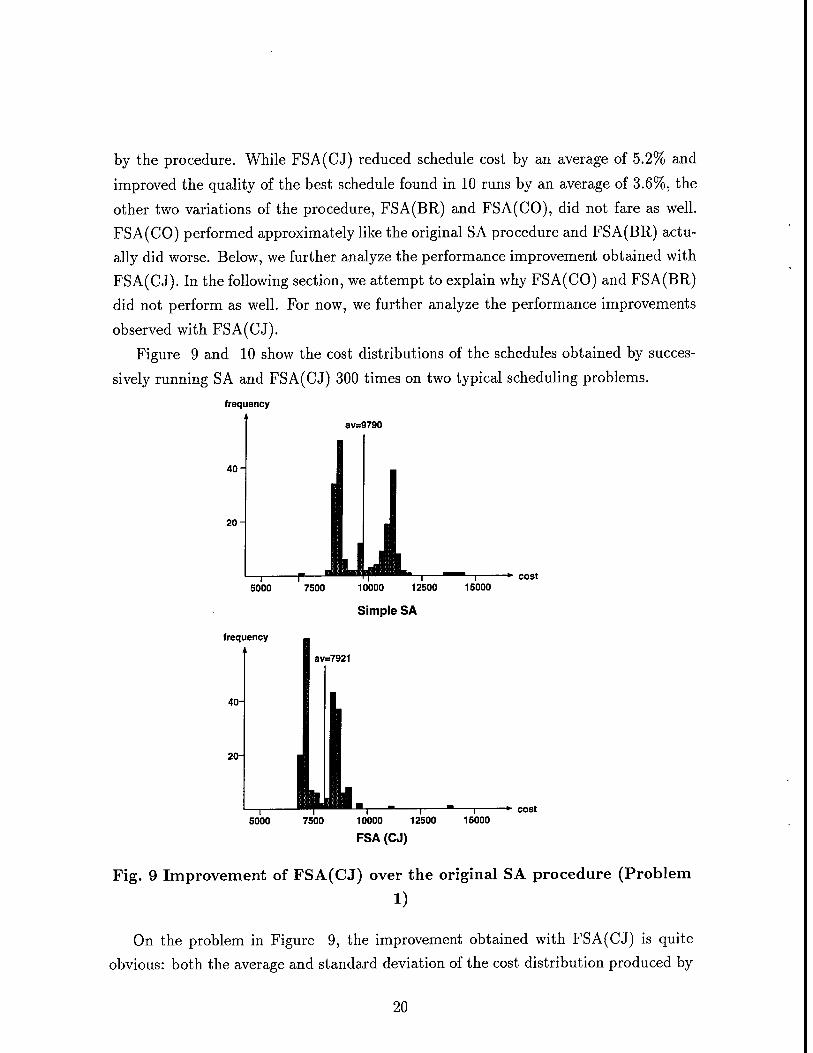
Figure 9 and 10 show the cost distributions of the schedules obtained by succes-
sively running SA and FSA(CJ) 300 times on two typical scheduling problems.
frequency
av=9790
cost S000 7500 10000 12500
Simple SA
15000
frequency
5000 7500 10000 12500
FSA (CJ)
—I ►■ cost 15000
Fig. 9 Improvement of FSA(CJ) over the original SA procedure (Problem
1)
On the problem in Figure 9, the improvement obtained with FSA(CJ) is quite
obvious: both the average and standard deviation of the cost distribution produced by
20
FSA(CJ) are lower than those of the original SA procedure. Accordingly, it appears
that for this problem the probability of getting trapped in a local optimum has been
greatly reduced. This in turn can translate in significant reductions in computation
time. For instance, while the original SA procedure would require an average of 2.5
runs to find a schedule with cost below 9000, FSA(CJ) would only require an average
of 1.1 run, a saving of more than 50%. To find a schedule of cost below 8000, FSA(CJ)
reduces computation time by more than 90%.
frequency
av=16128
40-
20
10000 15000 20000 25000 —I *• cost 30000
Simple SA frequency
40-
20-
av=15772
13 MfciL. 1 | iiinmi | ■i — -*■ cost 10000 15000 20000 25000
FSA (CJ)
30000
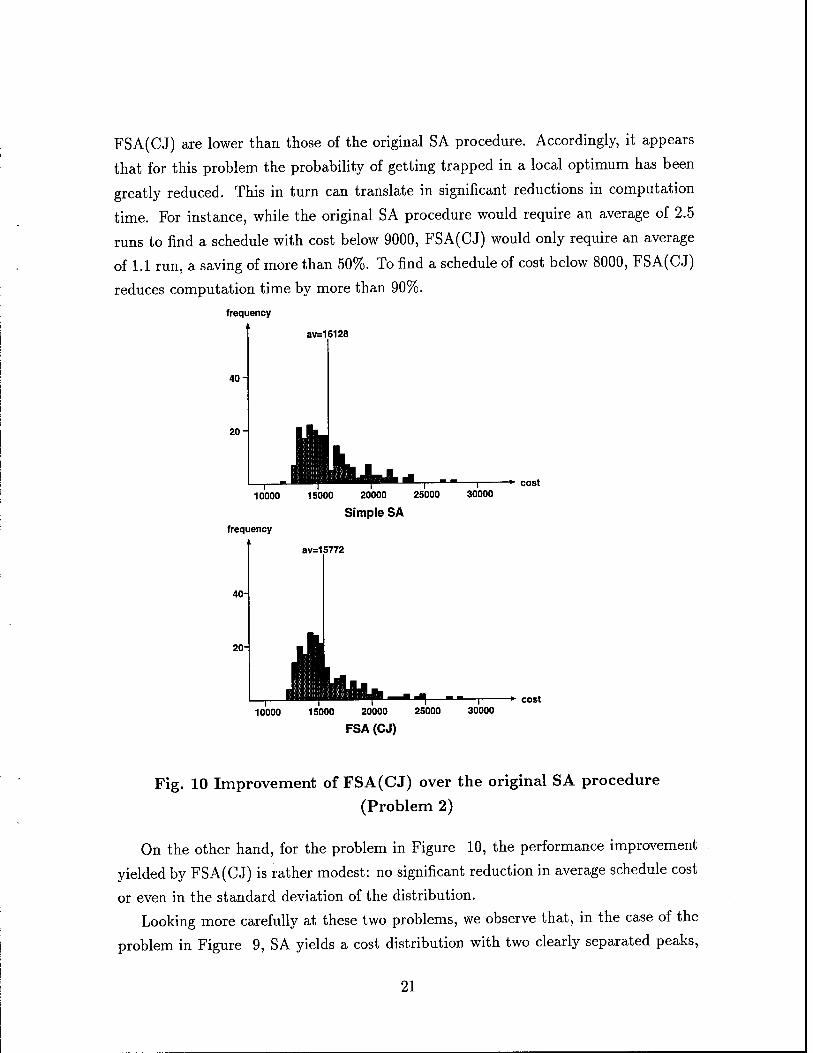
Fig. 10 Improvement of FSA(CJ) over the original SA procedure
(Problem 2)
On the other hand, for the problem in Figure 10, the performance improvement
yielded by FSA(CJ) is rather modest: no significant reduction in average schedule cost
or even in the standard deviation of the distribution.
Looking more carefully at these two problems, we observe that, in the case of the
problem in Figure 9, SA yields a cost distribution with two clearly separated peaks,
21
thereby suggesting that the procedure is often caught in local minima. In contrast, in
the case of the problem analyzed in Figure 10, the cost distribution obtained using the
original SA procedure is generally more compact. This would suggest that FSA(CJ)
is more effective in those situations where the original procedure is more likely to get
trapped in local optima.
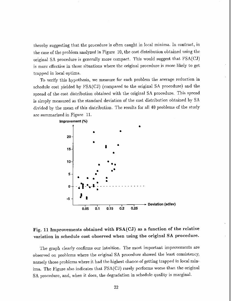
To verify this hypothesis, we measure for each problem the average reduction in
schedule cost yielded by FSA(CJ) (compared to the original SA procedure) and the
spread of the cost distribution obtained with the original SA procedure. This spread
is simply measured as the standard deviation of the cost distribution obtained by SA
divided by the mean of this distribution. The results for all 40 problems of the study
are summarized in Figure 11.
Improvement (%)
20
15-
10
5-
0.05 0.1 0.15 0.2 0.25 Deviation (sd/av)
Fig. 11 Improvements obtained with FSA(CJ) as a function of the relative
variation in schedule cost observed when using the original SA procedure.
The graph clearly confirms our intuition. The most important improvements are
observed on problems where the original SA procedure showed the least consistency,
namely those problems where it had the highest chance of getting trapped in local min-
ima. The Figure also indicates that FSA(CJ) rarely performs worse than the original
SA procedure, and, when it does, the degradation in schedule quality is marginal.
22
7 Further Analysis
If we are to apply FS A to other problems, we need to understand why some variations of
the procedure perform better than others. There are at least two ways of approaching
this question. One approach is to attempt to analyze the search procedure and the
neighborhood structure it relies on and try to understand how the choice of a given type
of subproblems influences the effectiveness of FSA on this specific class of scheduling
problems. This approach is probably the one a scheduling expert would be tempted to
follow. It could potentially lead to very insightful conclusions for the class of scheduling
problems of interest in this study. However, our purpose here is different, as we are
looking for insight that can possibly carry over to other domains. For this reason, we
take a different approach and limit our analysis to the external behavior of the search
procedure.
As pointed out at the beginning of Section 5, the early phase of a SA run, where
temperature is still high, generally determines whether the procedure gets caught in a
local minimum or not. Different neighborhood structures for a same class of problem
can possibly lead to different types of local minima. The nature of these local minima
can in turn affect the effectiveness of different problem decompositions in the FSA
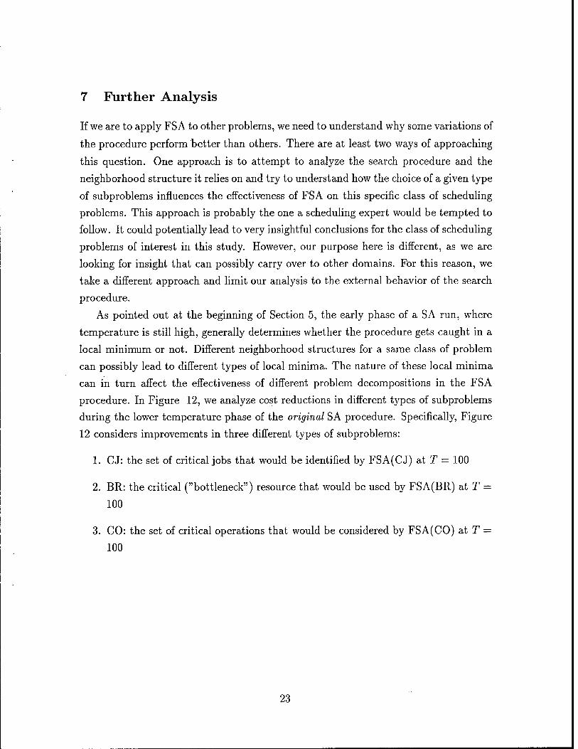
procedure. In Figure 12, we analyze cost reductions in different types of subproblems
during the lower temperature phase of the original SA procedure. Specifically, Figure
12 considers improvements in three different types of subproblems:
1. CJ: the set of critical jobs that would be identified by FSA(CJ) at T = 100
2. BR: the critical ("bottleneck") resource that would be used by FSA(BR) at T =
100
3. CO: the set of critical operations that would be considered by FSA(CO) at T =
100
23
cost
1.00
0.95-
0.90
0.85
0.80-
Temp. 100
Fig. 12 Changes of Cost in the Later Stage of SA
For each of these subproblems, Figure 12 plots the average variation in cost as-
sociated with these 3 subproblems as the temperature in the original SA procedure
is progressively lowered. The curve labeled " Totaf plots the cost variations of the
overall schedule as temperature decreases. The points in Figure 12 represent averages
taken over the set of 40 problems studied in Section 6 and over 10 runs of SA on each
problem.
Figure 12 indicates that, when using the original SA procedure, major inefhciences
in job schedules do not get corrected below temperature T = 100, while major ineffi-
ciencies at the level of critical resources or critical operations are still easy to eliminate.
This explains why FSA(CJ) is the variation that performs best: it is the one that best
matches the weaknesses of the original SA procedure. By working hard on eliminat-
ing inefficiencies at the level of critical jobs, FSA(CJ) reduces the chances that such
inefficiencies remain when the procedure reaches its lower temperature phase, a phase
when it is no longer effective at getting rid of these inefficiencies. For the same reason,
the BR curve suggests that FSA(BR) wastes its time getting rid of inefficiencies that
are still easy to eliminate in the lower temperature phase of the procedure, and hence
can be expected to perform poorly, as observed in the results presented in Section 6.
24
8 Summary and Concluding Remarks
In summary, the contribution of this work is twofold:
1. On the scheduling front, a SA procedure has been developed to solve job shop
scheduling problems with both tardiness and inventory costs. The procedure has
been shown to produce high quality solutions, reducing schedule cost by 28% over
a combination of 39 well-regarded dispatch rules and release policies (and by 20%
when the dispatch schedules are post-processed for optimal idle time insertion),
though at the expense of significant computational efforts.
2. To reduce the computational requirements of this procedure, a meta-heuristic
search procedure called Focused Simulated Annealing (FSA) search has been
developed. This procedure aims at reducing variability in the performance of SA
by dynamically focusing on the elimination of major inefficiencies in the solution.
The procedure works by dynamically inflating the costs associated with critical
subproblems and requires a decomposable objective function.
Three variations of FSA have been developed for the job shop scheduling problem
with tardiness and inventory costs. These variations of the procedure differ in the
type of subproblems they rely on: job subproblems, resource subproblems, or op-
eration subproblems. Experiments show that, with the right decomposition, FSA
can significantly improve solution quality especially on problems where search is
likely to get caught in local minima. Equivalently, for the same solution quality,
FSA can greatly reduce computation time over a regular SA search.
Our experiments also indicate that the performance of FSA critically depends
on the selection of a good decomposition of the objective function. An analy-
sis suggests that the most effective decompositions are those corresponding to
subproblems whose solutions are particularly difficult to improve during the low
temperature phase of the SA procedure. By focusing on inefficiencies at the level
of these subproblems, FSA can greatly reduce the chance of getting trapped in
local minima.
As is often the case in this type of study, many design alternatives remain to be
explored. Further work will also be required to assess the effectiveness of FSA or
FSA-like meta-heuristics in combination with more sophisticated SA procedures, e.g.
25
procedures incorporating some aspects of Tabu Search [9, 25, 19]. Like Strategic Oscil-
lation [7, 21, 10], FSA can be viewed as implementing a non-monotonic cooling sched-
ule, though selectively, by focusing on dynamically identified subproblems. Strategic
Oscillation could possibly also be exploited to control the value of ß, the parameter
used in our procedure to penalize precedence constraint violations within a job. Other
aspects of Tabu Search such as Target Analysis [8, 15], which, like FSA, adds a term
to the objective function to drive the procedure towards high quality solutions, would
also be worth comparing with and possibly incorporating in the existing procedure.
References
[1] Baker, K.R. "Introduction to Sequencing and Scheduling," Wiley, 1974.
[2] Cerny, V., "Thermodynamical Approach to the Traveling Salesman Problem: An
Efficient Simulation Algorithm," J. Opt. Theory Appl, Vol. 45, pp. 41-51, 1985.
[3] French, S. "Sequencing and Scheduling: An Introduction to the Mathematics of
the Job-Shop," Wiley, 1982.
[4] Fry,T., R. Amstrong and J. Blackstone "Minimizing Weighted Absolute Deviation
in Single Machine Scheduling," HE Transactions, Vol. 19, pp. 445-450, 1987.
[5] Garey, M. R. and Johnson, D. S. "Computers and Intractability: A Guide to the
Theory of NP-Completeness," Freeman and Co., 1979
[6] Garey M.R., R.E. Tarjan, and G. T. Wilfgong, "One-Processor Scheduling with
Symmetric Earliness and Tardiness Penalties," Mathematics of Operations Re-
search, Vol. 13, No. 2, pp. 330-348, 1988.
[7] Glover, F. "Heuristics for Integer Programming Using Surrogate Constraints,"
Decision Sciences, Vol. 8, No. 1, pp. 156-166, January 1977.
[8] Glover, F. "Future Paths for Integer Programming and Links to Artificial In-
telligence," Computer and Operations Research, Vol. 13, No. 5, pp. 533-549,
1986.
[9] Glover, F. "Tabu Thresholding: Improved Search by Non-Monotonic Trajecto-
ries," Technical Report, Graduate School of Business, University of Colorado,
Boulder, Colorado 80309-0419, 1993.
26
[10] Glover, F. and M. Laguna "Tabu Search," Chapter in Modern Heuristic Tech-
niques for Combinatorial Problems, pp. 70-150, Colin Reeves (Ed.), Blackwell
Scientific Publications, Oxford, 1992
[11] Holland J. "Adaptation in Natural and Artificial Systems" University of Michigan
Press, Ann Arbor, MI. 1975.
[12] Johnson, D. S., Aragon, C. R., McGeoch, L. A. and Schevon, C. "Optimization
by Simulated Annealing: Experimental Evaluation; Part I, Graph Partitioning"
Operations Research Vol. 37 no. 6, pp. 865-892, 1989
[13] Johnson, D. S., Aragon, C. R., McGeoch, L. A. and Schevon, C. "Optimization
by Simulated Annealing: Experimental Evaluation; Part II, Graph Coloring and
Number Partitioning" Operations Research Vol. 39 no. 3, pp. 378-406, 1991
[14] Kirkpatrick, S., Gelatt, C. D., and Vecchi, M. P., "Optimization by Simulated
Annealing," Science, Vol. 220, pp. 671-680, 1983.
[15] Laguna M. and F. Glover "Integrating Target Analysis and Tabu Search for
Improved Scheduling Systems," Expert Systems with Applications, Vol. 6, pp. 287-
297, 1993.
[16] Matsuo H., C.J. Suh, and R.S. Sullivan "A Controlled Search Simulated Annealing
Method for the General Jobshop Scheduling Problem" Tech. Report, "Dept. of
Management, The Univ. of Texas at Austin Austin, TX, 1988.
[17] Morton, T.E. "SCHED-STAR: A Price-Based Shop Scheduling Module," Journal
of Manufacturing and Operations Management, pp. 131-181, 1988.
[18] Morton, T.E. and Pentico, D.W. "Heuristic Scheduling Systems," Wiley Series
in Engineering and Technology Management, 1993
[19] Nowicki E. and C. Smutnicki "A Fast Taboo Search Algorithm for the Job Shop
Problem," Technical University of Wroclaw, Institute of Engineering Cybernetics,
ul. Janiszewskiego 1/17, 50-372 Wrocklaw, Poland, 1993.
[20] Osman,I.H., and Potts, C.N., "Simulated Annealing for Permutation Flow-Shop
Scheduling," OMEGA Int. J. of Mgmt Sei., Vol. 17, pp. 551-557, 1989.
27
[21] Osman, I.H. "Meta-Strategy Simulated Annealing and Tabu Search Algorithms
for the Vehicle Routing Problem" Annals of Operations Research, Vol. 41, pp. 421-
451, 1993.
[22] Ow, P.S. and T. Morton, "The Single Machine Early/Tardy Problem" Manage-
ment Science, Vol. 35, pp. 177-191, 1989.
[23] Sadeh, N. "Look-ahead Techniques for Micro-Opportunistic Job Shop Scheduling"
Ph.D. thesis, School of Computer Science, Carnegie Mellon University, Pittsburgh,
PA 15213, March 1991.
[24] Sadeh, N. "Micro-Opportunistic Scheduling: The Micro-Boss Factory scheduler"
Ch. 4, Intelligent Scheduling, Zweben and Fox (Ed.), Morgan Kaufmann Publish-
ers, 1994.
[25] Taillard, E. "Parallel Taboo Search Technique for the Job Shop Scheduling Prob-
lem," ORSA Journal on Computing, Vol. 6, pp. 108-117, 1994.
[26] Van Laarhoven, P.J., Aarts, E.H.L., and J.K. Lenstra "Job Shop Scheduling by
Simulated Annealing," Operations Research, Vol. 40, No. 1, pp. 113-125, 1992.
[27] Vepsalainen,A.P.J. and Morton, T.E. "Priority Rules for Job Shops with Weighted
Tardiness Costs," Management Science, Vol. 33, No. 8, pp. 1035-1047, 1987.
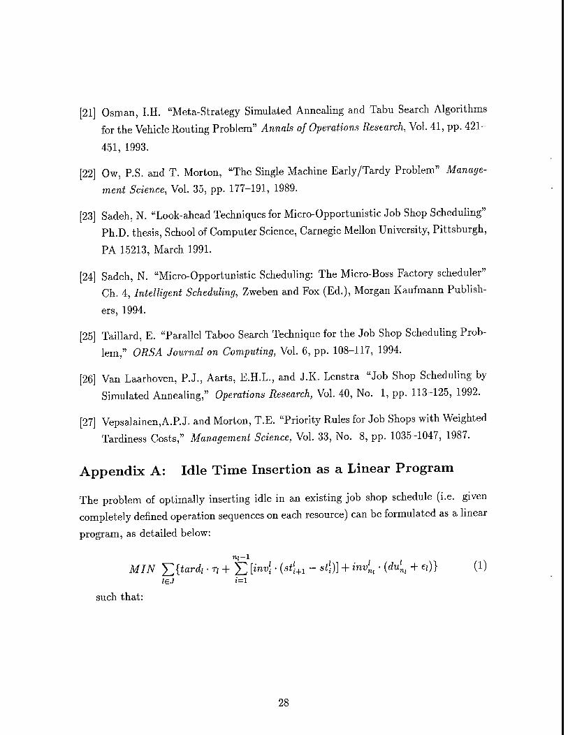
Appendix A: Idle Time Insertion as a Linear Program
The problem of optimally inserting idle in an existing job shop schedule (i.e. given
completely defined operation sequences on each resource) can be formulated as a linear
program, as detailed below:
nj—1
MIN Y,itardi ■T' + £ [inv'i • (54i - **!•)] + invlm • (du». + e<)} (1)
such that:
28
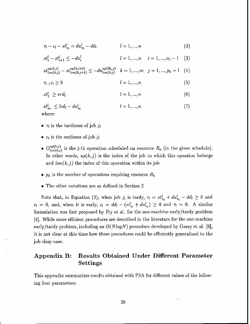
Ti-ti- stlni = dulni -ddi 1 = 1, ...,n (2)
st\ - stli+1 < -du\ / = l,...,n z' = l,...,n/-l (3)
,up(k,j) ,up(k,j+l) < ,up{Rk,i) , _ 1 • _ 1 _ 1 (A\ Stlow{k,j) Sllow(k,j+l) ^ aUlow(k,j) K-l,...,m J-l,...,Pfc i (4J
r/ ,e/ > 0 / = l,...,n (5)
.si^ > erdi l = l,...,n (6)
**»! <lcdi-du'ni / = l,...,n (7)
where:
• 77 is the tardiness of job j/
• e/ is the earliness of job ji
• Oj^r'kfi is the j-th operation scheduled on resource Rk (in the given schedule).
In other words, up(k,j) is the index of the job to which this opeation belongs
and low(k,j) the index of this operation within its job
• pk is the number of operations requiring resource Rk
• The other notations are as defined in Section 2
Note that, in Equation (2), when job ji is tardy, r\ — stlni + dulni — ddt > 0 and
e; = 0, and, when it is early, t\ = ddi — (stlni + dulni) > 0 and 77 = 0. A similar
formulation was first proposed by Fry et al. for the one-machine early/tardy problem
[4]. While more efficient procedures are described in the literature for the one-machine
early/tardy problem, including an O(NlogN) procedure developed by Garey et al. [6],
it is not clear at this time how these procedures could be efficiently generalized to the
job shop case.
Appendix B: Results Obtained Under Different Parameter Settings
This appendix summarizes results obtained with FSA for different values of the follow-
ing four parameters:
29
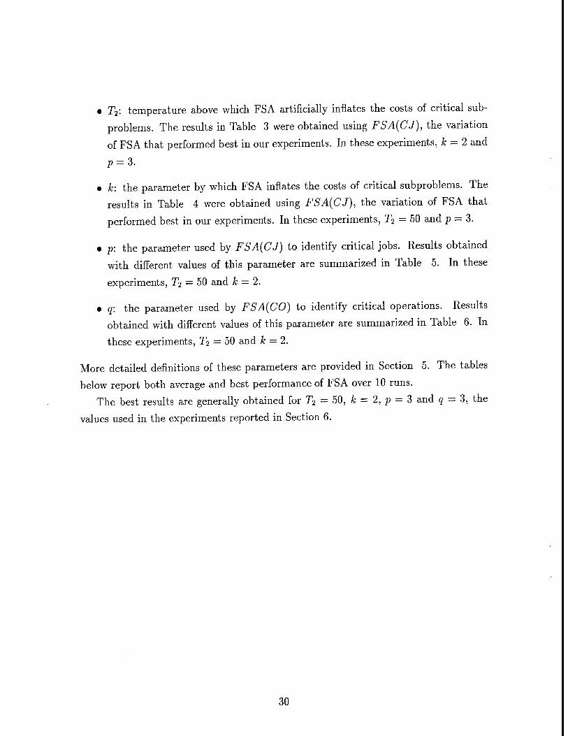
• T2: temperature above which FSA artificially inflates the costs of critical sub-
problems. The results in Table 3 were obtained using FSA(CJ), the variation
of FSA that performed best in our experiments. In these experiments, k = 2 and
p = 3.
• k: the parameter by which FSA inflates the costs of critical subproblems. The
results in Table 4 were obtained using FSA(CJ), the variation of FSA that
performed best in our experiments. In these experiments, T2 = 50 and p - 3.
• p: the parameter used by FSA(CJ) to identify critical jobs. Results obtained
with different values of this parameter are summarized in Table 5. In these
experiments, T2 = 50 and k = 2.
• q: the parameter used by FSA(CO) to identify critical operations. Results
obtained with different values of this parameter are summarized in Table 6. In
these experiments, T2 = 50 and k = 2.
More detailed definitions of these parameters are provided in Section 5. The tables
below report both average and best performance of FSA over 10 runs.
The best results are generally obtained for T2 = 50, k = 2, p = 3 and q = 3, the
values used in the experiments reported in Section 6.
30
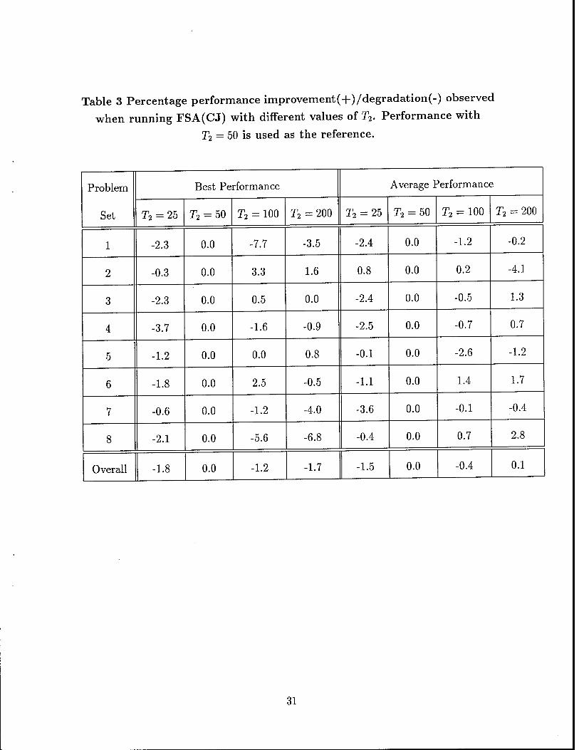
Table 3 Percentage performance improvement(+)/degradation(-) observed
when running FSA(CJ) with different values of T2. Performance with
T2 = 50 is used as the reference.
Problem
Set
Best Performance Average Performance
T2 = 25 r2 = 50 T2 = 100 T2 = 200 T2 = 25 T2 = 50 T2 = 100 T2 = 200
1 -2.3 0.0 -7.7 -3.5 -2.4 0.0 -1.2 -0.2
2 -0.3 0.0 3.3 1.6 0.8 0.0 0.2 -4.1
3 -2.3 0.0 0.5 0.0 -2.4 0.0 -0.5 1.3
4 -3.7 0.0 -1.6 -0.9 -2.5 0.0 -0.7 0.7
5 -1.2 0.0 0.0 0.8 -0.1 0.0 -2.6 -1.2
6 -1.8 0.0 2.5 -0.5 -1.1 0.0 1.4 1.7
7 -0.6 0.0 -1.2 -4.0 -3.6 0.0 -0.1 -0.4
8 -2.1 0.0 -5.6 -6.8 -0.4 0.0 0.7 2.8
Overall -1.8 0.0 -1.2 -1.7 -1.5 0.0 -0.4 0.1
31
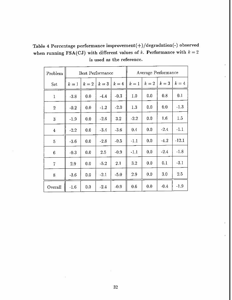
Table 4 Percentage performance improvement(+)/degradation(-) observed
when running FSA(CJ) with different values of k. Performance with k = 2
is used as the reference.
Problem
Set
Best Performance Average Performance
k = l k = 2 Jb = 3 k = i fc = l Jfe = 2 & = 3 k = A
1 -3.8 0.0 -4.4 -0.3 1.0 0.0 0.8 0.1
2 -0.2 0.0 -1.2 -2.0 1.3 0.0 0.0 -1.3
3 -1.9 0.0 -2.6 3.2 -2.2 0.0 1.6 1.5
4 -2.2 0.0 -3.4 -3.6 0.4 0.0 -2.4 -1.1
5 -3.6 0.0 -2.8 -0.5 -1.1 0.0 -4.2 -12.1
6 -0.3 0.0 2.5 -0.9 -1.1 0.0 -2.4 -1.8
7 2.9 0.0 -5.2 2.1 3.2 0.0 0.1 -3.1
8 -3.6 0.0 -2.1 -5.0 2.9 0.0 3.0 2.5
Overall -1.6 0.0 -2.4 -0.9 0.6 0.0 -0.4 -1.9
32
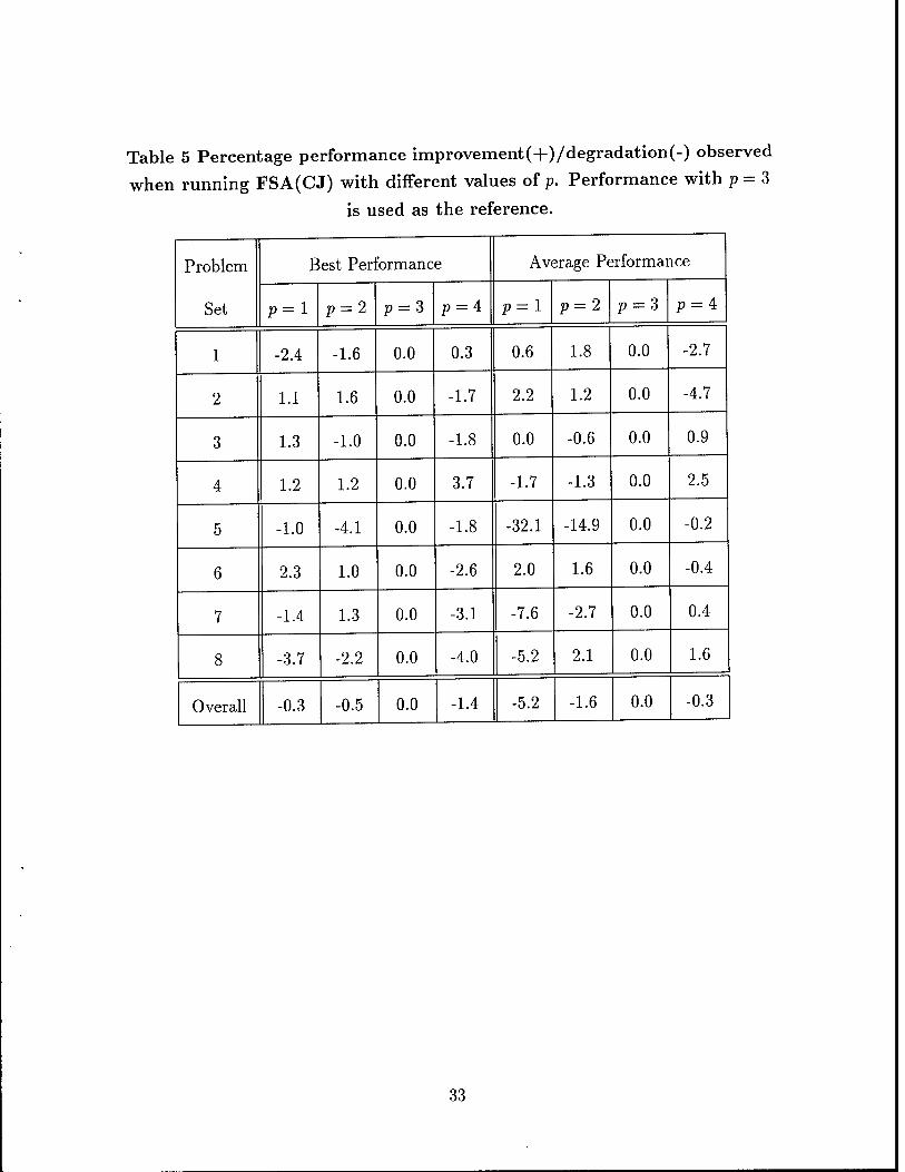
Table 5 Percentage performance improvement(+)/degradation(-) observed
when running FSA(CJ) with different values of p. Performance with p = 3
is used as the reference.
Problem
Set
Best Performance Average Performance
p = l p = 2 p = 3 p = 4 p=l p = 2 p = 3 p = 4
1 -2.4 -1.6 0.0 0.3 0.6 1.8 0.0 -2.7
2 1.1 1.6 0.0 -1.7 2.2 1.2 0.0 -4.7
3 1.3 -1.0 0.0 -1.8 0.0 -0.6 0.0 0.9
4 1.2 1.2 0.0 3.7 -1.7 -1.3 0.0 2.5
5 -1.0 -4.1 0.0 -1.8 -32.1 -14.9 0.0 -0.2
6 2.3 1.0 0.0 -2.6 2.0 1.6 0.0 -0.4
7 -1.4 1.3 0.0 -3.1 -7.6 -2.7 0.0 0.4
8 -3.7 -2.2 0.0 -4.0 -5.2 2.1 0.0 1.6
Overall -0.3 -0.5 0.0 -1.4 -5.2 -1.6 0.0 -0.3
33
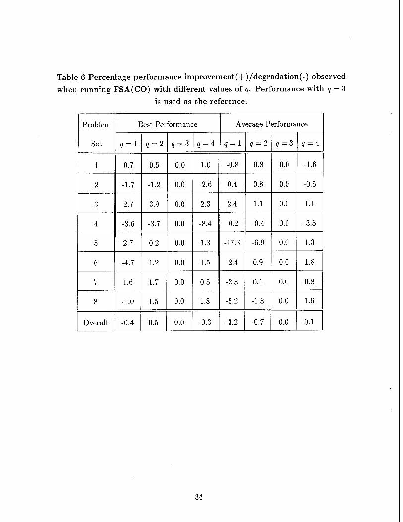
Table 6 Percentage performance improvement(+)/degradation(-) observed
when running FSA(CO) with different values of q. Performance with q = 3
is used as the reference.
Problem
Set
Best Performance Average Performance
q = l q = 2 q = 3 q = A q = l q = 2 q = 3 q = 4
1 0.7 0.5 0.0 1.0 -0.8 0.8 0.0 -1.6
2 -1.7 -1.2 0.0 -2.6 0.4 0.8 0.0 -0.5
3 2.7 3.9 0.0 2.3 2.4 1.1 0.0 1.1
4 -3.6 -3.7 0.0 -8.4 -0.2 -0.4 0.0 -3.5
5 2.7 0.2 0.0 1.3 -17.3 -6.9 0.0 1.3
6 -4.7 1.2 0.0 1.5 -2.4 0.9 0.0 1.8
7 1.6 1.7 0.0 0.5 -2.8 0.1 0.0 0.8
8 -1.0 1.5 0.0 1.8 -5.2 -1.8 0.0 1.6
Overall -0.4 0.5 0.0 -0.3 -3.2 -0.7 0.0 0.1
34