NTIA Report 83-134

FM SPECTRAL MODELING ANDFDM/FM SIMULATION PROGRAMS

CESAR A. FILIPPI

u.s. DEPARTMENT OF. COMMERCEMalcolm Baldrige, Secretary

David J. Markey, Assistant Secretaryfor Communications and Information

OCTOBER 1983

TABLE OF CONTENTS

Page

ABSTRACT.

SECTION 1 GENERAL INTRODUCTION •

SECTION 2 FM SPECTRAL MODELING AND GAUSSIAN REPRESENTATIONS.GAUSSIAN SPECTRAL APPROXIMATION PRINCIPLES •••••

Analysis of the Series Expansion Representation.Analysis of the 'Gaussian Spectral Approximation.

vi

1

3347

SECTION 3 RECTANGLE CONVOLIJTION PROGRAM FORFMSPECTRUM' SIMULATION • 11RECTANGLE CONVOLUTION PROGRAM PRINCIPLES • •• • • • •• 11RECTANGLE CONVOLUTION PROGRAM' RESULTS.. • • • • • • 14

SECTION 4 GENERALIZED FM SPECTRUM GENERATION PROGRAM • • 36DISCRETE FOURIER TRANSFORMS. • • • •• • .\ • • 38NUMBER OF. SAMPLES. • •• • • • • • • • • • 39BUTTERWORTH BASEBAND SPECTRUM SIMULATION. • 43PREEMPHASIS AND FM/PM CONVERSION SIMULATIONS • 50FDM/FM SPECTRAL SIMULATION RESULTS • • • • •

SECTION 5 SUMMARY AND DISCIJSSION OF RESULTS.

REFERENCES. . . . . . . . . .. . . . . . . . . . .66

71

APPENDIX A FM BANDWIDTH AND POWER DISTORTION • • •

APPENDIX B COMPARISON OF FDM/FM SPECTRAL SIMULATIONS • •

LIST OF TABLES

Table

72

77

1

2

Significant Terms (·Values of, n) vs" RMS Phase Deviation(S:>for Various Power Percentages • •• • • • • • • •

Residual Carrier Magnitudes in FM Spectra • •

iii

6

68

Figure

1

23(a)3(b)3(c)3(d)3(e)3(f)4(a)4(b)4(c)4(d)4(e)4(f)5(a)5(b)6(a)6(b)7(a)7(b)7(c)7(d)7(e)7(f)7(g)7(h)7(1)7(j)7(k)7(1)8(a)8(b)8(c)8(d)8(e)8(£)8(g)8(h)8(i)8(j)8(k)8(1 )9

10(a)10(b)

TABLE OF CONTENTS· (CONTINUED)

LIST OF FIGURES

Page

The Gaussian Envelope Approximation to the Poisson WeightingCoefficients • . • • • • • • • • • • • • • • • • • •• 8

Decomposition of Fn (f) into Fn (K) (f) segments 12Sum of N=5Weighted COIlvolutfons for S =0.2. • • • • • 15Sum of N=5 Weighted Convolutions for (3=0 .. 5. • • • • 15Sum of N=5 Weighted' Convolutiohsfor (3 =0. 7 • • • • • • • • • 16Sum of N=5 We-ig-ht::ed Convolutions for (3=1. O. • • • • .. .. • • 16Sum of N=9 Weighted Convolutions for S =2.0. • • • • •• 17Sum of N=17 Weighted Convolutions for (3=3.0 • • • • .. 17Case of N=5 'Weighted Convolutions for S =0.'2 • • 18Case of N=5 Weighted Convolutions for S =0.5 • • 18Case of N=5 Weighted Convolutions for S =0. 7. 19Case of N=5 Weighted' Convolutions .fors =1.'0. • • • • • 19Case of N=9 Weighted Convolutions for (3 '=2. O. • • • • • • • .. 20Case of N=17 Weighted Convolutions for S=3.0 • • • • • • • • 20Sum of Various Convolutions for S =2.0 • • • .. • • • • 21Sum of Various Convolutions for (3 =3.0 • • • • 21Case of Various Convolutions forS =2.0. • • • • • 22Case of Various Convolutions for (3 ==3.0. • • • • • • .. ••• 22Sum of N=5 Weighted Convolutions for ,(3=1.0 • • • ,,' '.. 24Sum of N=6 Weighted Convolutions for S=I.1 .. • • • • 24Sum of N=6 Weighted Convolutions forS ==1.2 • • • 25Sum of N=6 Weighted Convolutions for (3=1.3 • • • • • • • • •• 25Sum of N=6 Weighted Convolutions"' forS=I. 4 • • • • • • • •• 26Sum of N=8 Weighted Convolutions for S=I.5 • • • •• 26Sum of N=8 Weighted' "Convolutions for S =1.6'. • • .. .' • • 27Sum of N=8 Weighted Convolutions for S=1. 7 .. .. 27Sum of N=9 Weighted Convolutions for S =1.8 • • • •• 28Sum of N=9 Weighted Convolutions for S=1.9. • • • • •• 28Sum of N=9 Weighted Convolutions for (3 =2.0 • 29Sum of N=17 Weighted Convolutions forS=3.0 • ••• • • 29Case of N= 5 Weighted Convolutions for [3 =1. O. 30Case of N= 6 Weighted Convolutions for S=1.1. • • •• 30Case of N= '6 ,W'eighted Convolutions for S =1.2 .. .. 31Case of N= 6 Weighted Convolutions forS =1.3 • • • • • 31Case of N= 6 Weighted Convolutions for S =1 •.4 32Case of N= 8 Weighted Convolutions for (3'=1• .5 • • • •• 32Case of N= 8 Weighted Convolutions forS =1.6 • .. • • • • • • • •• 33Case of N= 8 Weighted Convolutions forS =1. 7 • • •• 33Case of N= 9 Weighted Convolutions for S ::1.8 • • • • 34Case of N= 9 Weighted Convolutions for S =1. 9 • • • • • • • 34Case of N= 9 Weighted Convolutions for S =2.0 • 35Case of N= 17 Weighted Convolutions for S=3.0 • • • • 35Generalized FM Spectrum Generation. • • • • • 37Inverse DFT Realization via Direct DFT. • • • • • • • •• 40Inverse DFT Realization for Real Even Symmetry.. • •• 40

iv

11(a)11(b)1213(a)13(b)13(c)13(d)13(e)13(f)13(g)13(h)141516(a)

16(b)

17(a)17(b)17(c)17(d)17(e)17(f)17(g)17(h)18(a)18(b)18(c)18(d)18(e)18(f)18(g)18(h)18(i)18(j)18(k)18(1)19

TABLE OF CONTENTS(CONTINUED)

LIST OF FIGURES

Inverse Transform Simulation with Dimensional Analogy • • • • •Direct Transform Simulation with Dimensional Analogy.Butterworth Powe,r Density Spectra • • • • • • • • •.• • • • •Central Butterworth Correlation Function:' 'First Case. • • • •Central Butterworth Correlation Function: Se'condCase ••• '.Central Butterworth Correlation Function: Third Case.Central Butterworth Correlation Function: Fourth Case • '. • •Noncentral Butterworth Correlation Function: First Case •Noncentral Butterworth Correlation·Function: Second Case.Noncentral Butterwort'h Correlation Function: Third Case • •Noncentral Butterwort'h Correlation Function: Fourth Case.Preemphasized Baseband Spectrum with Rectangle Input •••Equivalent Phase Modulating Spectrum with Rectangle Input • • • • •Equivalent Phase, Modulating Spectrum with P=50 and P=100

Butterworth Inputs • ••••••••••••••••••Equivalent Phase~ Modulating Spectrum with P=10 and P=20

Butterworth Inputs • • • • •• • • • • • • • • • • • • • • • • •FDM/FM Spectrum for m=O.10•••••••••••FDM/FM Spectrum for m=O.33. • • • • • • • •FDM/FM Spectrum for m=O.5 •FDM/FM Spectrum for m=1.0FDM/FM Spectrum for m=2.0 • • • • •FDM/FM Spectrum for m=J.O • • • •FDM/FM Spectrum for m=4.0 ••••••FDM/FM Spectrum for m=5.0 •••• • •FDM/FM Spectrum of 1800-Channel Bell TD2 System •FDM/FM Spectrum of 2400-Channel Bell TH System.FDM/FM Spectrum of 1500-Channel Bell TD2 SystemFDM/FM Spectrum of 1500-Channel AT&T System •FDM/FM Spectrum of 1800-Channel AT&T System • •FDM/FM Spectrum of 1200-Channel AT&T System •FDM/FM Spectrum of 360-Channel AT&T System.FDM/FM Spectrum of 600-Channel AT&T System.FDM/FM Spectrum of 360-Channel Western Union SystemFDM/FM Spectrum of 420-Channel Western Union System •FDM/FM Spectrum of 180-Channel Western Union SystemFDM/FM Spectrum of 120-Channel Western Union System • •Conversion Factor (S/m) as a Function of Baseband Parameter ( ) • •

v

Page

41414546464747484849495252

53

535555565657575858595960606161626263 .63646469

ABSTRACT

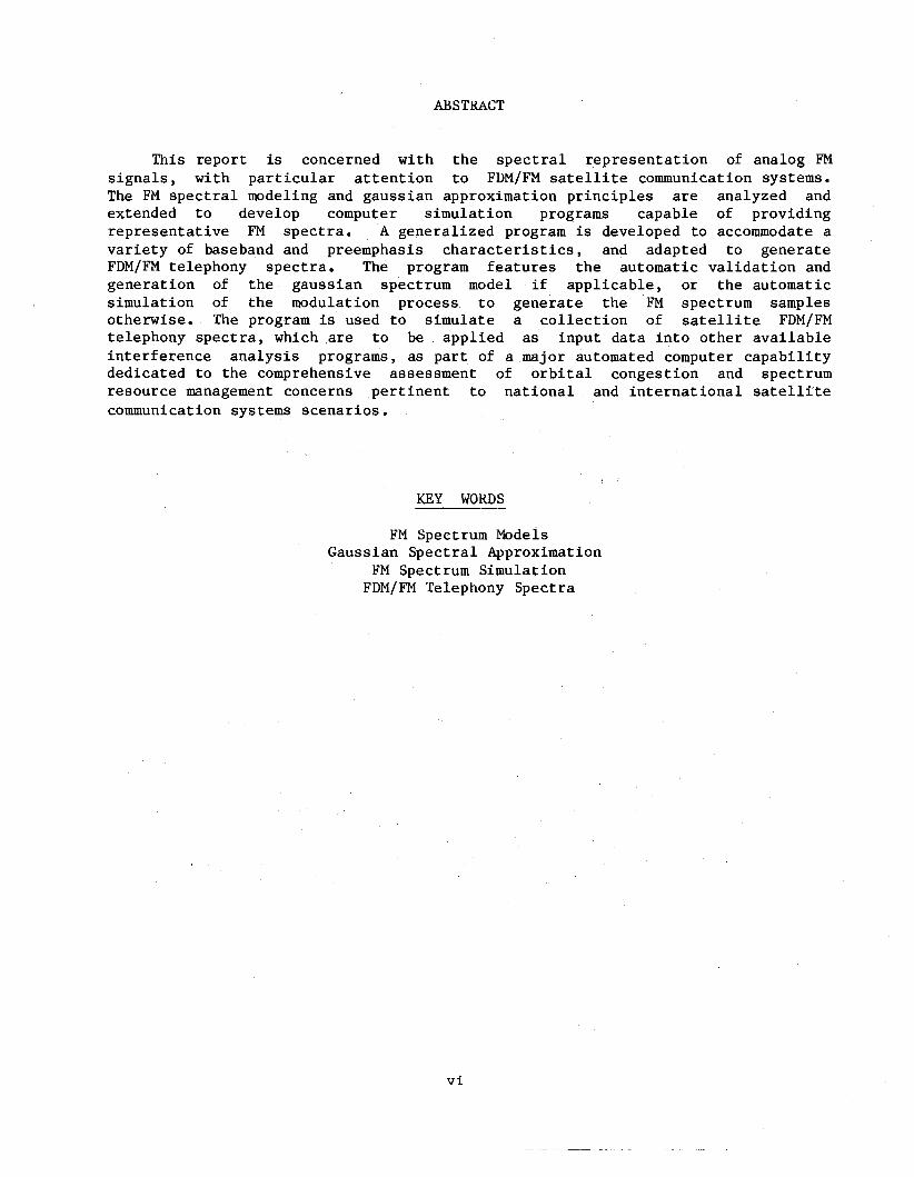
This report is concerned with the spectral representation of analog FMsignals, with particular attention to FDM/FM satellite communication systems.The FM spectral modeling and gaussian approximation principles are analyzed andextended to develop computer simulation programs capable of providingrepresentative FM spectra. A generalized program is developed to accommodate avariety of baseband and preemphasis characteristics, and adapted to generateFDM/FM telephony spectra. The program features the automatic validation andgeneration of the gaussian spectrum model if applicable, or the automaticsimulation of the modulation process to generate the FM spectrum samplesotherwise. The program is used to simulate a collection of satellite FDM/FMtelephony spectra, which .are to be applied as input data into other availableinterference analysis programs, as part of a major automated computer capabilitydedicated to the comprehensive assessment of orbital congestion and spectrumresource management concerns pertinent to national and international satellitecommunication systems scenarios.

KEY WORDS

FM Spectrum ModelsGaussian Spectral Approximation

FM Spectrum SimulationFDM/FM Telephony Spectra

vi

SECTION 1

GENERAL INTRODUCTION

The National Telecommunications and Information Administration (NTIA) isresponsible for managing the radio spectrum allocated to the U.S. FederalGovernment. Part of :NTIA' s responsibility is to: .....establish policiesconcerning spectrum assignment, allocation and use, and provide the variousDepartments and agencies wittl guidance to assure that their conduct oftelecommunications activities is consistent with these policies" (Department ofCommerce, 1980). In support of these requirements, I'lTIA performs spectrumresource assessments to identify existing or potential spectrum utilization andcompatibility problems among the' telecommunication systems of various departmentsand agencies. NTIA also provides recommendations to resolve any spectrum usageor allocation conflicts, and to improve the spectrum management functions andprocedures.

NTIA is engaged in the development of an automated computer capability to beused by the Federal Government for the comprehensive assessment of ~national andinternational satellite communication systelus. The program will feature bothinterference evaluation and logical optimization of a varying systems population,thus supporting ttle orbit and spectrum resource management functions. Theeffective coexistence of multiple satellite systems and service signaltransmissions represents a critical concern from the orbital congestion,communications interference and service reliability standpoints.

The orbital and spectrum congestion introduces unwanted signals into theantennas and receivers of dedicated satellites and earth stations. Theinterfering signals processed by the satellite transponder and earth stationreceiver equipment ultimately appear as degradation effects on the desired outputinformation, whether it be analog messages or digital symbols. The linkgeometries and power budgets of the various satellite systems establish desiredand interference signal levels at tIle receiving station inputs, which need to beconverted into output degradation effects so as to guide the logical assessmentof the operational scenarios.

The development of receiver transfer characteristics to evaluate theinterference degradation effects requires accurate spectral representations ofthe signals involved (Jeruchim and Kane, 1970; Pontano, et aI, 1973; Das andSharp, 1975). Many existing models and formulations contain simplE~ qualitativeassumptions or restricted parametric conditions as validity constra-ints, withmore accurate spectral representations needed to employ the available results ordevelop new ones as required. For example, the compact forluulations availablefor analog FM applications are - conditioned on extreme 11igh or low modulationindices, with representation uncertainties hindering their usage in intermediateindex situations.

The sections tllat follow 'are concerned with the spectral representation foranalog FM applications. The spectral modeling and gaussian approximationprinciples are first identified in Section 2, and then extended to developeffective F~I spectrum simulation programs capable of resolving the modelil1gconcerns and providing representative FM spectra. The programs developed consistof a specific one dedicated to a particular baseband modulation, plus a

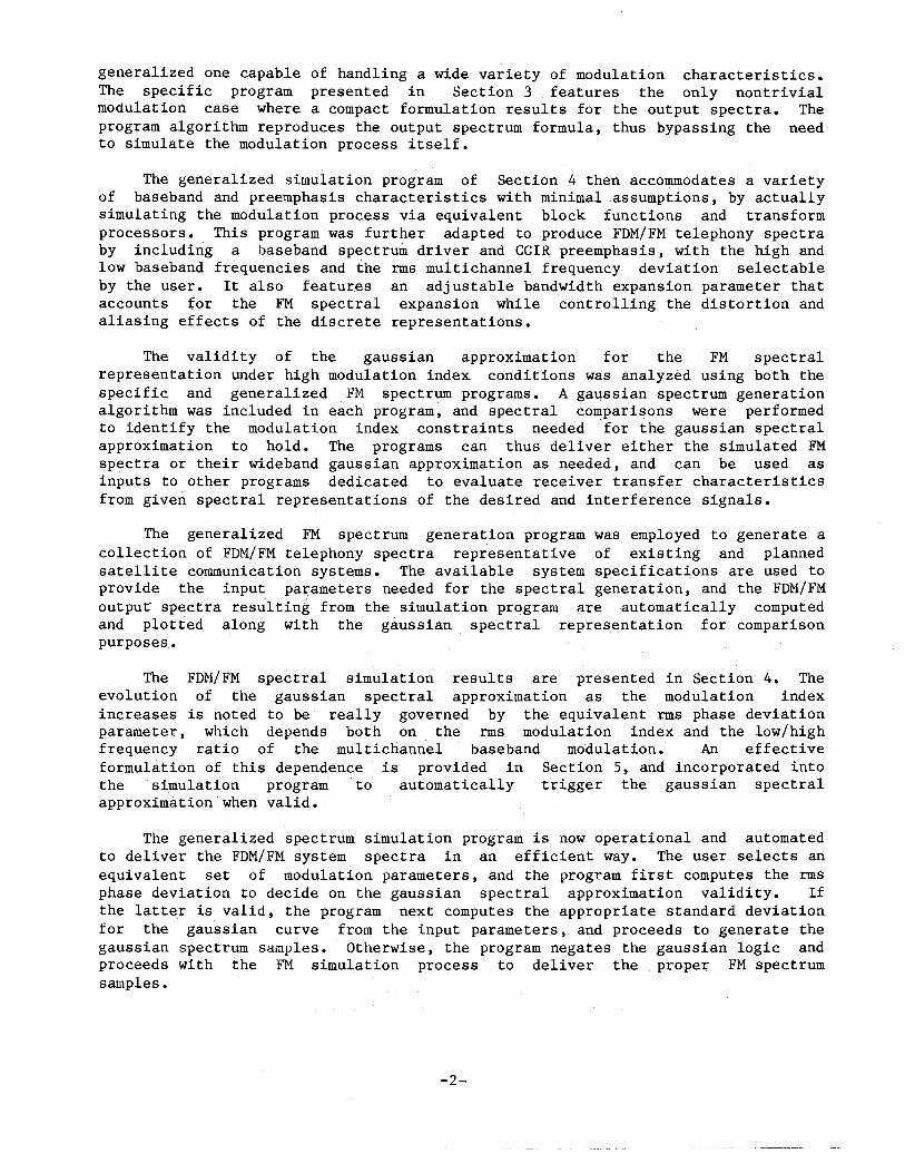
generalized one capable of handling a wide variety of modulation characteristics.The specific program presented in Section 3 ,features the only nontrivialmodulation case where a compact formulation results for the output spectra. Theprogram algorithm reproduces the output spectrum formula, thus bypassing the needto simulate thetn0dulation process itself.

The generalized simulation program of Section 4 then accommodates a varietyof baseband and preemphasis c"haracteristics with minimal assumptions , by actuallysimulating the modulation process via equivalent block functions and transformprocessors. Tllis program was further adCipted to produce FDM/FM telephony spectraby including a baseband spectrum driver and CCIR preemphasis, with the high andlow baseband frequencies and the rms multichannel frequency deviation selectableby the user. It also featur,es an adjustableband,widthexpansion parameter thataccounts for the EM spectral expansion while controlling the·distortion andaliasing effects of the discrete representations.

The validity of the gaussian approximation for the FM spectralrepresentation under high modulation index conditions was analyzed using both thespecific and generalized Frvl spectrum programs. A gaussian spectrum generationalgorithm was included in each program, and spectral comparisons were performedto identify the modulation index constraints needed" for the gaussian spectralapproximation to hold. The programs can thus deliver either the simulated FMspectra or their wideband gaussian approximation as needed, and can be used asinputs to other programs dedicated to evaluate receiver transfer characteristicsfrom given spectral representations of the c;lesired and interference signals.

The generalized FM spectrum generation program was. employed to generate acollection ofFDM/FM telephony spectra representative of existing and plannedsatellite communication systems. The available system specifications are used toprovide the input pat;ameters needed for the spectral generation, and the FDM/FMoutput" spectra resulting from the simulation 'prqgram are automatically computedand plotted along with the gaussian spectral repres~ntation for comparisonpurposes.

The FDM/FM spectral simulation results are pI:"esented in Section 4. Theevolution of the gaussian spectral approximation as the modulation indexincreases is noted to be really governed by t'he equivalentrms phase deviationparameter, which depends both on the rms modulation index and thelow/highfrequ'ency ratio of the multichannel baseband modulation. An effectiveformulation of this dependence is provided in Section 5,andincorporated intothe simulation program to automatically trigger the gaussian spectralapproximation when valid.

The generalized spectrum simulation program is now operational and automatedto deliver the FDM/FM system spectra in an efficient way. The user selects anequivalent set of modulation parameters, and t-he program first computes the rmsphase deviation to decide on the gaussian spectral approximation validity. Ifthe latte,r is valid, the program next computes the appropriate standard deviationfor the gaussian curve from the input parameters, and proceeds to generate thegaussian spectrum saulples. Otherwise) the program negates the gaussian logic andproceeds with the 'Fr.1 simulation 'process to deliver the proper FM spectrumsanlples.

-2-

SECTIQN.2

FM SPECTRAL MODELING AND GAUSSIAN REPRESENTATI,ONS

The FM signal spectrum models presently employed only have a compactformulation in certain cases. At low modulation. ,indices, the FM output spectrumis effectively approximated by a discrete carrier ,component plus adouble-sideband continuous spectrum. The latter has the same shape as theequivalentlowpass spectrum that phase modulates the carrier under low indexconditions. In parti'cular~ such' lowpass spectrum will be identical to the inputbaseband spectrum when i.deal FM preemphasis (parabolic power weighting) isemployed.

At hig'h modulation indices, the FM output spectrum is. characterized by asmall discrete carrier component plus a predominant continuous gaussian spectrumcentered around the carrier component. The relative power distribution betweenthese discrete and continuous components is uniquely specified by the rms phasedeviation. The only other information needed to specify the FM output spectrum isthen the gaussian standard deviation or variance parameter, which controls theeffective width of the continuous gaussian portion of the spectrum. Thisparameter has been formulated in terms of the rms phase or frequency deviationemployed, and' renders the FM spectrum model charac~erization under high indexconditions.

The gaussian spectrum, model is assumed to hold regardless of the inputbaseband spectrum or preemphasis characteristic, as long as the hi,gh modulationindex exists. However, the identification of what represents a 'high indexcondition remains somewhat arbitrary. Also, the variety of baseband spectra,preemphasis characteristics,modulation indices and frequency deviations employedin the different FMsignals of interest spans a considerable range of spectralshapes and parameter values, which hinders the spectral approximation evaluation.Hence, the FM spectral modeling issue should be given due attention to assureaccurate signal characterizatiolD.s and permit reliable interference an,alyses.

Another pertinent issue consists of the parametric value assignment in thegaussian spectrum model. The standard deviation param~ter in the gaussianformula is sometimes specified from the rms phase deviation ina PM formulation,and sometimes from the rms frequency, deviation in an FMformulation, as discussedin what follows. The conversion is tractable in most baseband cases withoutpreemphasis, but the pr1eemphasized baseband cases can lead to computationaldifficulties. The preemphasis network can be designed to preserve the rms phaseor frequency deviation but' not both in general, and the evaluation of the one notbeing preserved may be difficult yet required if, the gaussian spectralrepresentation is to be employed.

GAUSSIAN SPECTRAL APPROXIl~TION PRINCIPLES

The original principl4~ supporting the gauasian spectral approximation underhigh index conditions is based on Woodward's theorem (Blackman and McAlpine,1969). It states that the limiting form of the FM power density spectrum as theindex increases is given by the probability distribution of the instantaneous

-3-

modulating frequency. Hence, the assumption of gaussian statistics in thebaseband modulating signal (with arbitrary spectrum) dir~ctly induces a limitinggaussian FM spectrum for high in'dices under the theorem, with the gaussianstandard deviation given by the rms frequency deviation,.

The modulation index magnitude needed for an effecti"e representation by thegaussian spectrum was riot resolved in Woodward's theorem. The identification ofcrossover index bounds is ,hindered by the fact that they may vary ~ith themodulating signal spectrum, since all Woodward's theorem provides is for agaussian spectrum convergence in the l~mit. There have been some theoreticalextensions of the theorem, with the maIn results consisting of autocorrelation orspectrum error estimates or bounds as a function of the rms index or frequencydeviation, as well as some spectral simulation results for specific basebandspectra. However, the error performance and criteria ,were found to vary inprediction accu'racy capability with the modulatiQo index ,value and the basebandspectral shaping involved (Blackman and McAlpine, ,1969;; Algazi, 1968)'.

Another princIple supporting the gaussian spectral approximation under highindex conditions relies on a pow~r series expansion (Middleton's expansion) ofthe autocorrelation function of the modulated signal, again assuming basebandgaussian statistics but arbitrary spectrum (Abramson, 1963). The series termsare each characterized by a different power of the autocorrelation function ofthe equivalent baseband phase modulation including any preemphasis effects. Theautocorrelation function of the frequency modulated signal becomes a weigh,tedsuperposition of these powers of the autocorrelation function of the phasemodulating signal.

The power density spectrum <?f the modulated signal becomes a weig'htedsuperposition of spectral terms obtained from the series ~xpansion. Each spectralterm consists of an n-th order convolution of the baseband phase modulatingspectrum, with the number of cQnvolutions· varying .with the series terms. Eachspectral convolution is then weighted by a different coeff,icient and superposedto yield the resultant FM spectrum. The gaussian spectral approximationessentially consists of motivating how the weighted superposition of differentspectral shapes cart be IIlanipulated under high index conditions to result in a.gaussian spectrum (Abramson,' 1963).

Analysis of the SeriesExpans~op Represen~ati<?n

The equivalent p'hase modulating signal is assumed to be a stationarygaussian process with zero mean and fixed standard deviation (6 radians). Itmodulates a' sinusoidal carrier of fixed amplitude (A) and frequency (w c radiansper second), so that the correlation function ~(t) of the modulated signal y(t)can be expressed in terms of the correlation function Rx(t) of the modulatingsignal x(t) as (Abramson, 1963):

- [R{o) ...R (t) ]• e x x • cos 4.\.c t

-4-

(1)

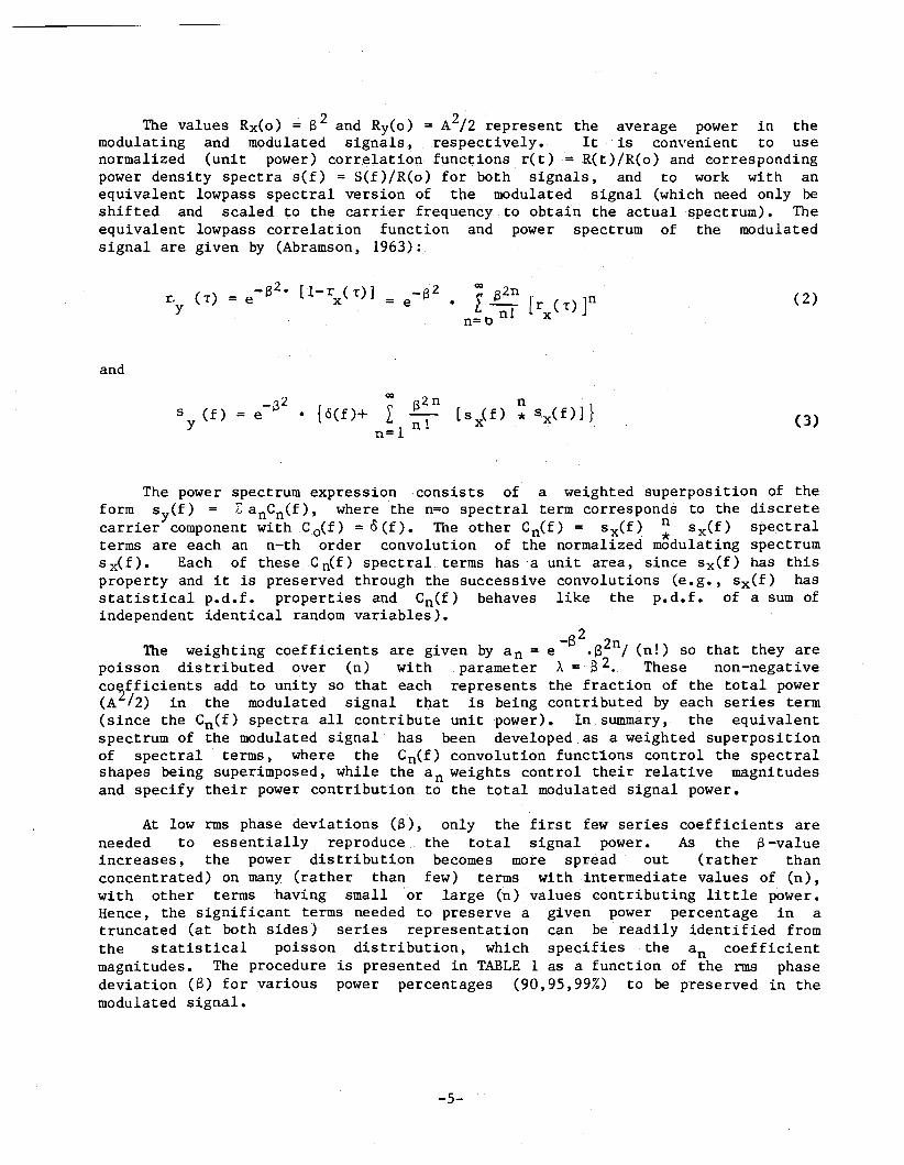
The values R){(o) = f3 2 and Ry(o) = A2/2 represent the average power in themodulating and modulated signals, respect1v~ly. It is con~renient to usenormalized (unit power) correJ..ationfunc~ionsr(t)'=R( t) /R(o) and correspondingpower density spectra s(f) = S(f)/R(o) for both signals, and to work with anequivalent lowpass spectral version of the modulated signal (which need only beshifted and scaled to the carrier. frequency to obtain t:he actual '-spectrum). Theequivalent lowpass correlatio'n function and power spectrum of the modulatedsignal are given by (Abramson, 1963):,

(2)

and

(3)

At low rms phase de'viations (a), only the first few series coefficients areneeded to essentially reproduce the total signal power. As the a-valueincreases, the power distribution becomes more spread out (rather thanconcentrated) on many (rather than few) terms with intermediate values of (n),with other terms having small or large (n) values contributing little power.Hence, the significant terms .. needed.to preserve a given power percentage in atruncated (at both sides) series representation' can be readily identified fromthe statistical poisson distribution, which specifies the an coefficientmagnitudes. The procedure is presented in TABLE 1 as a function of the rms phasedeviation (a) for various power percentages (90,95,99%) to be preserved in themodulated signal.

-5-

TABLE 1

SIGNIFICANT TERMS (VALUES OF n) VS RMS PHASE DEVIATION ( (3)

FOR VARIOUS POWER PERCENTAGES

A= 82

f3 n(90%} n(95%) n(99%)

1 1.000 0-2 0-4 0-4

2 1.414 0-5 0-5 0-6

3 1.732 1-6 0-6 0-8

4 2.000 1-7 1-8 0-9

5 2.236 2-9 1-9 0-11

6 2.449 2-10 2-11 1-13

7 2.646 3-11 2-12 1-14

8 2.828 4-13 3-13 2-16

9 3.000 4-13 4-15 2-17

10 3.162 5-15 4-16 3-18

11 3.317 6-16 5-17 4-20

12 3.464 7-18 6-19 4-21

13 3.606 7-18 6-20 5-23

14 3.742 8-20 7-21 5-24

15 3.873 9-21 8-23 6-25

16 4.000 10-23 9-24 7-27

17 4.123 10-.23 9-25 7-28

18 4.243 11-24 10-26 8-29

19 4.359 12-.26 11-27 9-31

20 4.472 13-27 12-29 10-32

-6-

These results can be directly used for the selection of the number of seriesterms and spectral convolutions needed in a truncated repr,esentation orsimulation of ,the modulated signal spectrum. The entries in TABLE 1 show that upto nine terms besides the carrier component may be needed for S<2 radians ,withthe number reaching 17, 27, 32 terms as the index increases to 3, 4, 5 radians.Some spectral simulation:s of FDMjFM .telephony are available in the openIiterature for S= 1 to 5 iradians; but ' etllploying only ten series terms in thetruncated representation (Ferri.s,' 1968). The results of TABLE 1 illustrate thatnot only more terms are actually needed for such range, but that the first tenterms have a negligible or secondary contribut.ion once the rms phase deviation

exceeds four radians.

Analysis of thei·.Gaussia:n Spectral Approximation

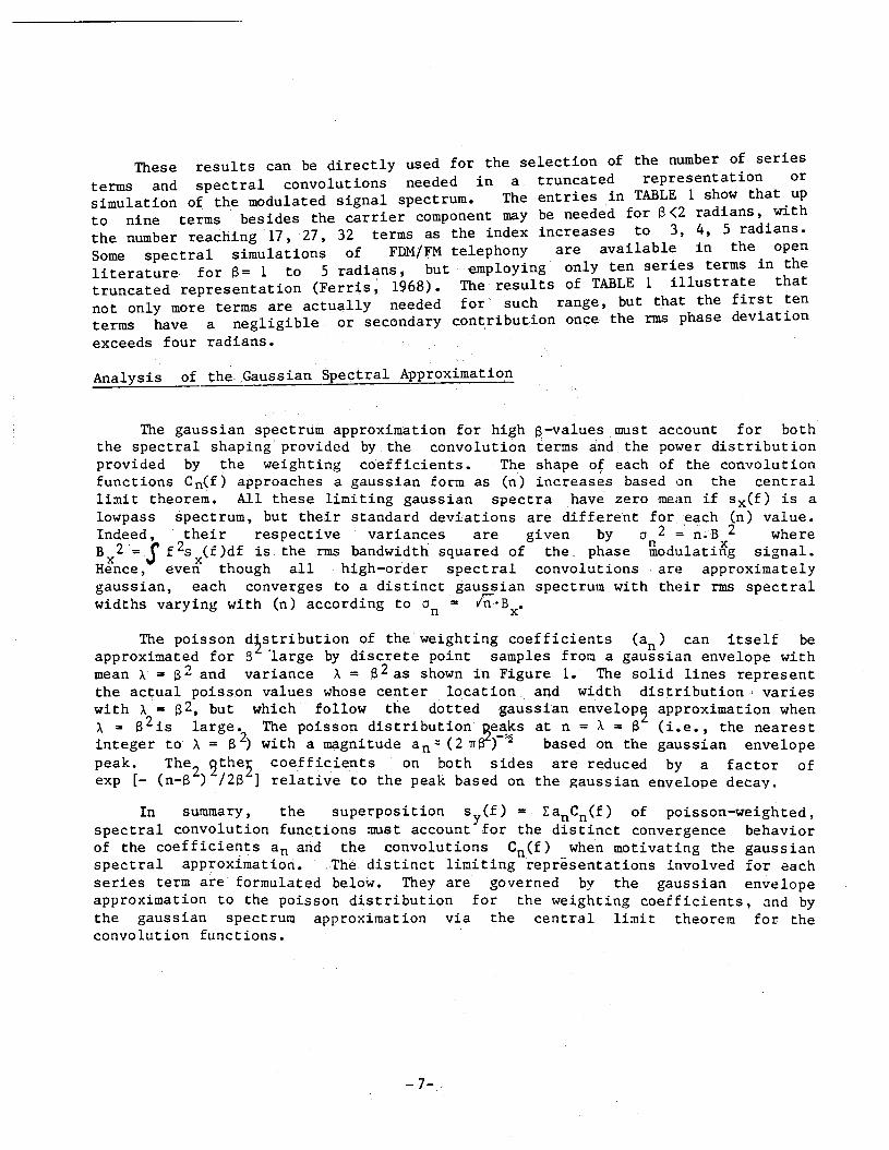
The gaussian,spectrum approximation for high a-values ;must aceount for boththe spectral shaping'provided by the convolution term.sand the power distributionprovided by the weighting co'efficients. The shape of each of the convolutionfunctions Cn(f) approaches a gaussian form as (n) increas.esbased on the centrallimit theoreni. All t,heselimitinggaussian spectra have zero 'mean if sx{f) is alowpass spectrum, but their standard deviations are different for ,each (n) value.Indeed, their respec~tive ,variances are given by 0 2 =' n;B 2 whereB .. Z = S f 2s (f )df is . the rms bandwidth squared of the phase lftod\llatiHg signal.Hince ,e,ve~ though' all high-order spectral convolutions arE! approximatelygaussian~ each converges to a distinctgallssian spectrum with thE!ir rInS spectralwidths varying with (n) according to a = /tr,. B •n x

The poisson d~stribution of the weighting coefficients ,(an) can itself beapproximated for B 'large by discrete point samples from a gaussian envelope withmean A = 6 2 and variance A = B2 as shown in Figure 1. The solid lines representtile actual poisson values whose center .locat·ion and. width distribution! varieswith A = 82, but which ~ follow the dotted gaussian enveloP2 approximation whenA =- a2 is large. The poisson distribution ~e~ksat n = A = B (i.e., the nearestinteger to A = a2) with a magnitude an:: (2 lT8'~)-~ based on the gaussian envelopepeak. The2 ~the~ coefficie'nts '. on both sides are reduced by a factor ofexp [- (n-a ) /28 ] relative to the peak based on the gauss'ian envE!lope decay.

In summary, the superposition Sy{£) = ranCn(f) of poisson-weighted,spectral convolution functions must account for the distinct convergence behaviorof the coefficiellts an arid the:convolutions, Cn,(f) when motivating the gaussianspectral appro~imation. ~Th~.distinct limiting repr~sentations involved for eachseries "term are formul.atedbelow. They are governed by the gaus'sian envelopeapproximation to the poisson distributio,n for the weighting coefficients, and bythe gaussian spectrum approximation via the central limit theorem for theconvolution functions.

-7-

ContinuousGaussianEnvelope

Discret·ePoissontines

/

n=O

2n=S -1 2n=(3 +1

Figure 1. The Gaussian. Envelope Approxitnat~on to th~ PoissonlA]eighting Coefficients.

Poisson" Lines:

G~ussian·Envelope:

an

a zn

[ e-S:~s2n I ]

[e-t::::>12S

12for n ., a

and S2 large

-8-

a' C (f)n, n ' (4a)

(4b)

... ....

gaussian envelope gau~sian spectrum

approximation to approximation to

poisson-distributed n-th order

weighting coefficients convolution function2(for a large) (for n large)

The fact that each c:onvolutionfuncti'on Cn(£) -a.pproaches a distinct gaussianshape does not imply that their weighted superposition can also 'be assumed to begaussian., .The following rationale is al'so -involved in motivating the gaussiansp.ectral representation:

(a) Only those series termscoefficients and need be kept.

with?nZS-'will ha'1e' signific~antweighting

(b) Their associated Cn(f) functions can all be approximated by the samecurve by letting n = .(32 for all terms kept, which removes the spectral widthvariation with n.

(c) ~e series has now been reduced to (Ean).C(f), where C(f) = C (f) withn = (3 , and the sum of coefficients can be approximated by unity si8'ce onlysignificant terms were kept.,

(d) The series has nowfunction with standardan = F· Bx •

become 'just Cff), which is a gaussian speCtraldeviation a =(3·B as obtained by setting n = (3 in

x

(e) The equivalent lowpass powe-r spectrum of the modulated signal is thusapproximated by

sy(f)

-9-

(5)

This development emphasizes that the gauss1anspectral representation of themodulated signal under high rms phase deviation conditions is not astraightforward approximati'on. It not only requires that~ each convolution termCn(f) be gaussian approximated, but also that the weighting coefficientsa n selectively cooperate to remove the sp'ectral width variations with Ii andapproximate a single gauss1ap spectrum from the superposition of distinctapproximately gaussian spectra. Also, the; stal1ciard deviation a =13 • Bx of thegaussian spectral approximation can be noted to bea function of the rmsphasedeviation (13) and the rmsbandwidth (~x) of the equivalent phase modulatingsignal.

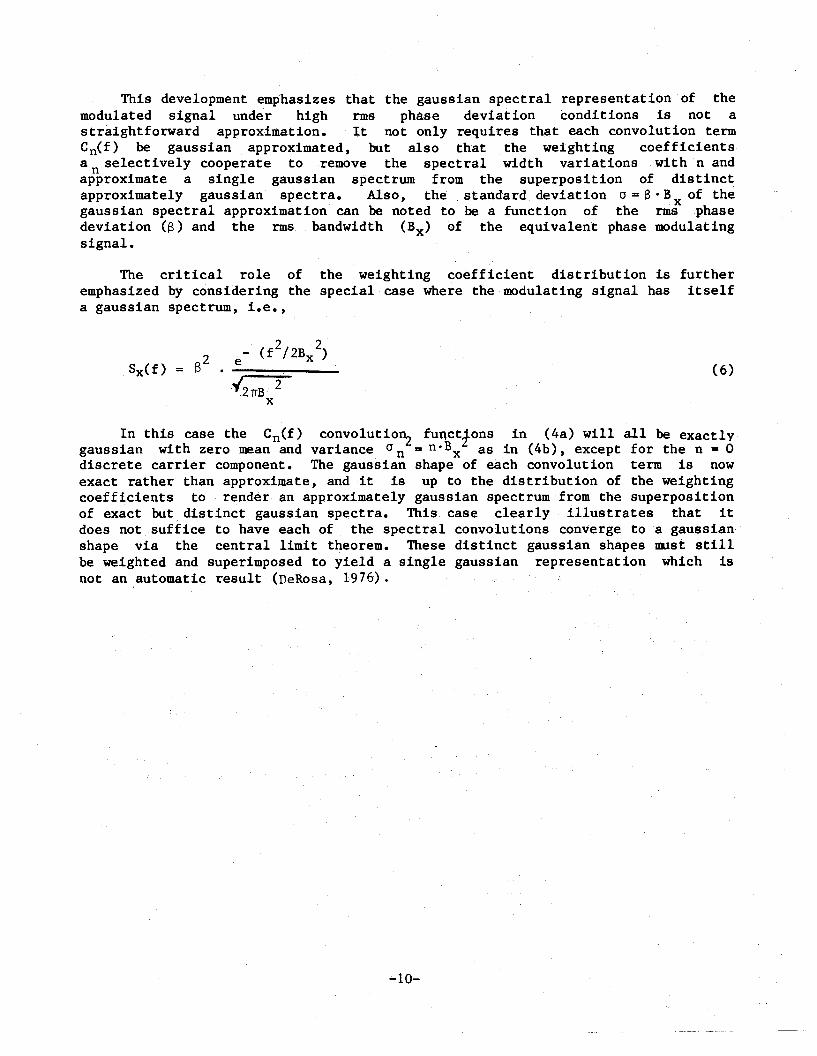
The critical role of the weighting coefficient distribution is furtheremphasized by considering the special case where the modulating signal has itselfa gaussian spectrum, i.e.,

Sx(f)- (f2/2B 2)e x

"ZTrB Zx

(6)

In this case the Cn(f) corivolutio~ fUt\ctfons 1n (4a) will all be exactlygaussian with zero me,an 'and variance an = n.Bx as in (4b), ,except for the n = 0discrete carrier component. The gaussian shape of each convolution term is nowexact rather than approximate, and it is up to the distribution of the weightingcoefficients to render, an approximately' gaus'sian spec.trum .from the superpositionof exact but distinct gaussian spectra. This case clearly illustrates that itdoes not suffice to have each of the spectral convolutions converge to' 'a gaussian·shape via the central limit theorem. These distinct gaussian shapes DI.lst stillbe weighted and superimposed to yield a single gaussian representation which isnot an ,automati~ result (DeRosa" 1976) •

...10-

SECTION 3

RECTANGLE CONVOLUTION PROGRAM FOR FM SPECTRUM SIMULATION

The previous sections h.ave shown that the gaussian spectral approximationfor FM signals remains to be" validated insofar as the modulation indexconstraints and the baseband sp'ectrum dependence is concerned. A possibleapproach consists of comparing the gauss~an spectrum to the actual FM spectrumobtained from theoretica~·i· siniulati.on or empirical results. l

• One tractable casethat features a -compact theoretical formulation, compatible with computersimulation i~pleme~tation is cons~dered in' this section,4t

The case in question ,consists of a lowpass rectangular baseband spectrumthat phase modulates the sinusoidal carrier. This case corresponds to aparabolic frequency modulating spectrum; so that it can represent a rectangularbaseband spectrum followed by a parabolic preemphasis characteristic in PMapP11·Cjt1·ons, The nor........a11·zed ......'h~"'" ........od.·· 1n ... ;n·,.,. """."'."t-u"- ;,... ..... ;'TT"'"""' .....'TT """,'+:\ - ,/T.T• W . PUQi:)C W u..J..Q .. ..J..15 i:)pc\" L W ..J..i:) 5..J..VCU uy i:),A\.L J - .J./ n

for If ~ \'112, and the interes t is to derive the n-th order convolutions en (f) ofthis spectrunl, so as to forrl1 their weighted superposition with fhe coefficientdistribution governed by the rms phase deviation assumed.

A computer program W(1~; developed at NTI...AA. to simulate the compactmathematical formulatiol1 representing the n-th order spec.tral convolutions Cn (f).There is no need to simulate the actual convolution operations, as exactexpressions for Cn(f) are avaj~lable in an iterative form for any (n) "'lalue. Thecomputer simulation only requires the development of effective algorithms toimplement the iterations involved, and to generate the (an) weightingcoefficients so as to form the LanCn(f) superposition representing the FM signalspectrum. The gaussiaIl spectral approximation of (5) was also implemented so asto compare it to the actual FM spectrum obtained.

THE RECTANGLE CONVOLUTION PROGRAM PRINCIPLES

A transformation to a uni,t' width ;rectangle (W == 1) defined over the unitinterval (0, 1) is convenie.nf to exploit available theoretical results. If then-th order convolution '£unc.tion obtained under these conditions is denoted byFn(f), with n=l corresponding to ~he initial rectangle, then the transformation

(7)

yields the convolution functions of interest. The argument shift by n/2 centersall the Fn(f/W) functions at the origin, and the scaling of the frequencyvariable and the function magnitude removes the unit width premise.

\-

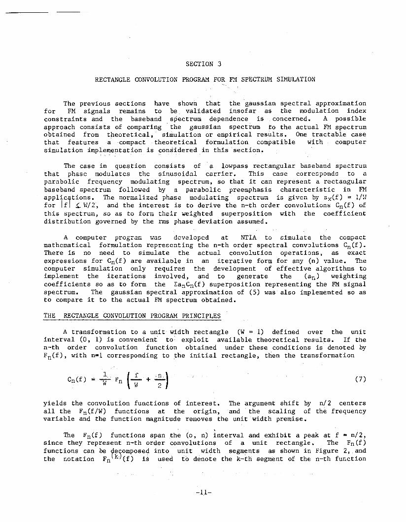
The Fn(f) functions span the (0, n) interval and exhibit a peak at f = n/2,since they represent n-th order convolutions of a unit rectangle. The Fn(f)functions can be de~ompose~ into unit ,width.' segments as shown in Figure 2, andthe notation Fn~k)(f) is used to denote the k-th segment of the~ n-th function

~11-

F (f)n

o 1 2 3

n-12

n2

n+12

n-2 n-1 n (f)

F (f)n

Case ofn-odd: Peak Occurs at Middle of Midsegment

o 1 2 3 n-2 n-1 n (f)

n-12

n2

n+12

Figure 2.

Case of n-even: PeakOcclJ.rsat Boundary 'of Midsegments

Decomposition of F (f) into F (k) (£) segments.n n

-12-

wherel ~ k ~n. The' mot:ivatfon for th'is decomposition is that there existcompact express"ions for the 'Fn (k) (f) segments, with an fterative formulationover (k)' and (n) that caIibe exploit~din,a computer "simulation to' generate anentire function from on'e' segmel1t ' (k' itera'ti'ori) -'and 'to superpose the weightedfunctions to oqtain the spectr\lIll. (n iteration).

~The general express:ion for' an a;rbitrary" k-th, s~gment (1 ~k ~n) of anar1?itrary n-th function (n 2. 1)' is given by (Cramer, '1945).:

I

(n-l)!

k-l

I:j=O

(f-j )n-l k-1 < f < k- (8)

and the segment iteration over(k) follows as

F(k+l}(f) = F(k) (f) +n 'n (n-I)t

(f - k)n-l (9)

The validity of these formulas was verified by independently evaluating thefirst' few convolution functions to match" and th~~ performing induction proofsover (k) and(n) to ,check the general expressions. The formulas reproduced theconvolution functions in'que~tion, and the induction relation was verified usingbinom~~l coefficient properti~s (Feller, 1968).

The Fn (f) functions are. symmetric about their peak at f = nl 2, so there isonly ne~d to ev,aluate the. s~gments on one side of the peak to generate thefunction. The evaluation was performed bydevelopirtg a digital computer programthat simulated the formulas alid produced point 'samples of one-'half of eachfunction. The program also included the appropriate shifting of these samples toboth sides of the origin, sQas to deliver thesylnnietric left and right samplesnee4ed to generate the en (f) functions centered" at the origin.

The weighted superposition of the Cn(f) functions as shifted v~rsions of the,Fifi(f) fUIlctionscatl beaccompli~he~ ,in two ,ways. "One approach consists of firstgenerating the, entire shift~d functions and then adding them on a weighted pointl.?a.sis..P1ismethod requir,es cCl~e,tul sele~ti()n of 'the sampling ,points in theup-shifted Fn (f), functions to as'sure the overlap of the shifted samples fromdiffe'rent 'funct'ions.. Al10ther apptoacl), co,nsists of first fixing the shiftedsample points and only adding the specific weighted sampl~s needed from eachunshifted function.

Both methods were investigated for computer simul~tion, and the first onewas implemented in the prograDl. An effective overlap of the shifted samples fromdifferent functions was provided by taking an even, number of samples per segmentin the unshifted functions. The peak of the unshifted functions lies at the

-13-

middle .of ~hemidsegmentif{n)i$oddandat the boundary between two symmetricmidsegments if (n) is even., The use of an even sampling rate per segment assuresthe peak .coveragerega~,d~ess, 0,£" whether(n) is . odd or 'even, and the shi'ftedsample overlaps b~9ome'assuredw~en the ,pea~: ove~lapsare provi,d~d.

The weighting coefficients an were generated by the program for a given rmsphase deviation (a ) using, the poisson distribution .formula. The number ofcoefficients needed wasestablisl,1ed according to TABLE 1 as a function of8for agiven ~ower preservation criterion. The n = o carrier component with magnitudeexp (-8 ) was independently evaluated, since the weighted superposition algorithmexcluded such discrete component to avoid the impulse simulation. A dBtransformation of the discrete and continuous ~pectral magnitudes was alsoimplemented.

THE RECTANGLE CONVOLUTION PROGRAM RESULTS

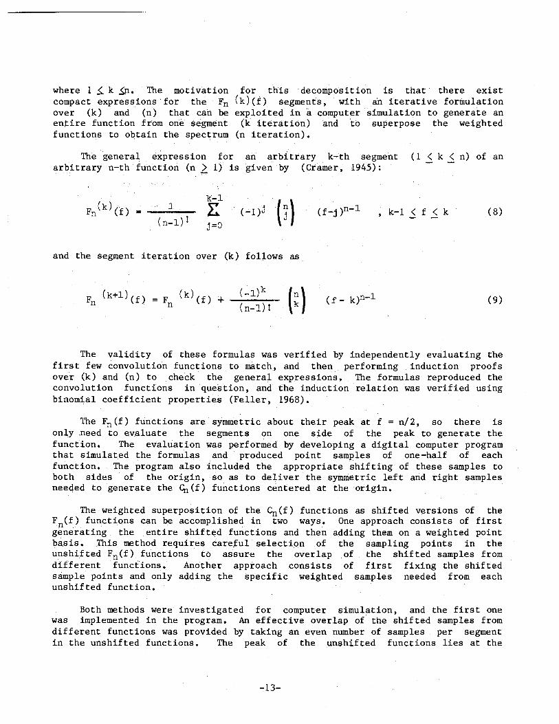
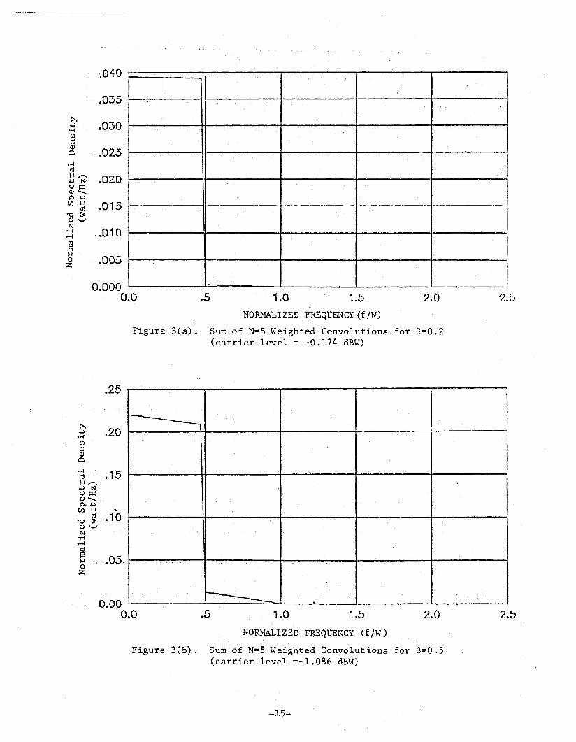
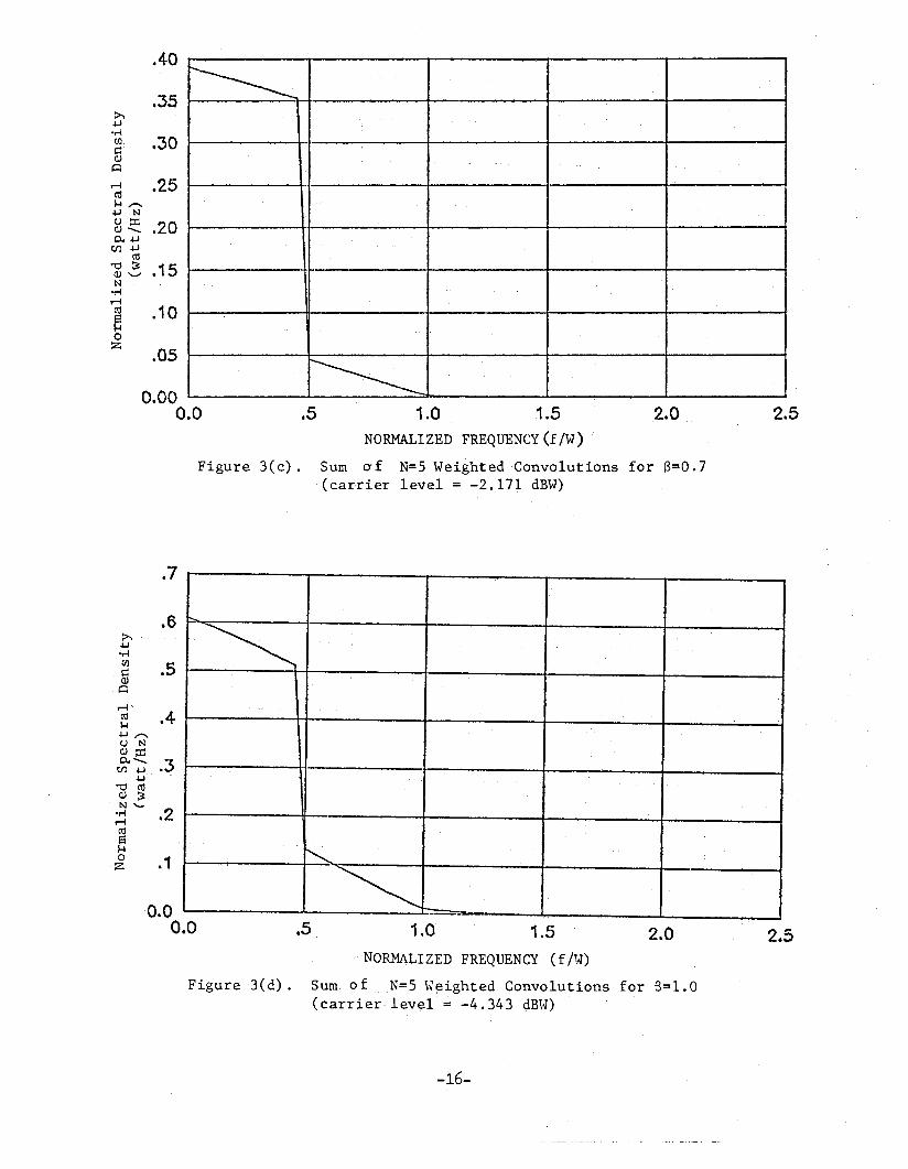
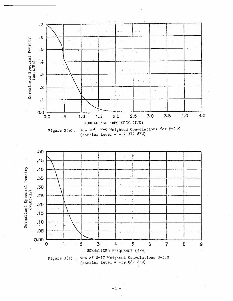
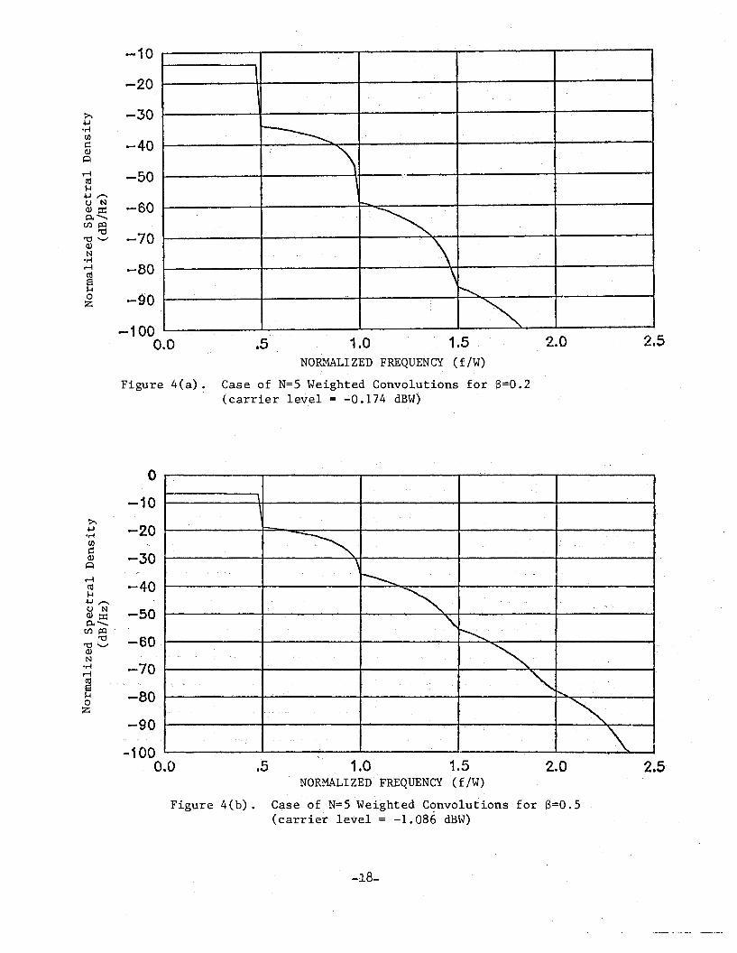
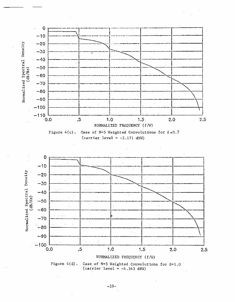
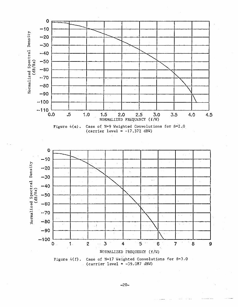
The results of the simulation program just described are presented in thissection. The normalized FM spectral densities for various a-values are shown 1nFigures 3( a) to 3( f ) with linear scale and in Figures 4( a) to 4( f) in dB scale.The first set of figures illustrates' the ,variation of the FM spectrum fromrectangular to gaussian shape as B increases, while the second set serves todiscriminate the spectral tail magnitudes obtained. The'rms phase deviation,isgiven by 13 radians, and the carrier component magnitude of - 132 log10e dB isindicated in all plots.

The number of spectral convolutions (series ter,ms) employed wa~ selectedaccording to ,TABLE 1 to provide., a .'. 99 perce'nt pow~r ,preservation in theFM spectrum. A minimum of five convolu~ions was perforllled for those cases whereless would have sufficed. The effectiveness of the procedure was also verifiedby performing more and less convolutions than required, and verifying that nosignificant differences were .. obtained with: the extra convolutions.

Some typical verification results are pr~sented in Figures, 5(a) and S(b),where the nom~nal number of convolutions required is indicated in the legend. Asmaller number of convolutions proves to be insufficient for the nominalreproduction, whereas a iar'ger number match'es the nominal reproduction in ,thesignificant spectral region. The differential effects of the extra convolutionsappear in the spectral tail regions as eVidenc'ed by the dB plots' of Figures 6(a)and 6(b).

The i,nterest is to compare the gaussian spectr,umapproximationto the FMs.,ilectrum obtained .,via the spectral convol,ution ... series. 'The baseband phasemodulatingspec~rum'.has;the normalized form·sx(f)"= l/W fori fl.::.w/2, .from whichthe rms bandwidth follows as Bx= wl:m.' 'Hence,the' gaussian spectrumapproximation has a standard' "deviaton given by ...e1=.~ ~ Bx =t3WI'v'~ so that thegaussian formula (5) becomes

s (f) =y -1T

-14-

( 10)

.04-0

.035 ~------++--------+--------+-------t-------i

.030

.025

.015

.010

.005

2.52.0.5 1.0 1.5NORMALIZED FREQ-UENCY (f /W)

Figure 3(a). Sum of N=5Weighted Convolutions for 8=0.2(carrier level = -0.174 dBW)

0.0000.0

...

.25

~

.20~.~

en

~~

M .15(1j,....;-..+-J Nc.J ::x::Q)~p..~

Cf.) +J ...(1j .10

~ ~Q) '-"N

.,-4

M(1j

s .0-5-,....0z

0.000.0 .5 1.0 1.5 2.0 2.5

NORMALIZED FREQUENCY (f/W)

Figure 3(b).. Sunl of N=-S Weighted Convol.ut ions for 8=0,,5(carrier level =-1.086dBW)

-1C)-

2.52.0i.S 1.01.5NORMALIZED FREQUENCY(f!W)

Figure 3(c). Sum 0'£ N=S Weighted 'C'onvolutions for S=0.7(carrier level:::; -2.171 dBW)

~

--

I,

~0.000.0

.40

.35~

+J-,-4en .30S::'(1)

~

~ .25roJ-I,-..+J N(J p:: .20(1) ..........p..+JU)+J

roPtj ~ .15(1),-,N

-r-f~ro .10sJ-I0z

.05

"""'-

~

:

-~

~~~

.7

.6~+J-,-4en .5s::(1)~

Hro .4~

+J "'"'"'t.) N(1) p::p... .......... .3CI) +J..

+JPtj

&(1)

N'-.2-I""'f

~

roS~0 .1z

'0.00.0 .5 1.0 1.5 2.0 2.5

NORMALIZED FREQUENCY (f/W)

Figure '3(d). Sum· of N=5 W~ightedConvolutions for e=1.0(carrier,level,= -4.343 dB~.J)

-16-

-- I

-' .

.......-- -------

,~ ".-,. .--

.--..... --

'\.

I~

~~.I4.54.03.5.5 1.0 1.5 2.0 2.-5 3.0

NORMALIZED FREQUENCY (f!W)

Figure 3( e). SumO f N=9 W'eighted Convolutions for S=2.'0(c·arrier level = -17.372dBW)

·7

0.00.0

1'\

'\'\\\,

\

\,. \

,'" \'"~

9871 2' "3 4 56NOltl1ALIZED .FREQUENCY (f!W)

Figure 3(f). Sum, ofN=17We~ghtedConvolutions 6=3.0(car:r;ie~ level := ~39.087 dBW)

-17-

2.52.0.5

\\

~

\ ,---~

\\

,', ~

~1.0 1.5

NORMALI ZED FREQUENCY ( f /W)

Figure 4(a) ~ Case of N=5 Weighted Convolutions for S=O.2(carrier level = ~O.174 dBW)

-1000.0

--10

--20

~ .-30+oJ-r-t

CJ)

t:: -40QJ0

M ....50co~+oJ ".......U N -60QJ::dp..""'"C/)~

"0-70"0 '-'

QJN

-r-tM -80cos~0 -90z

t-._.-..~,-~.,~

~

"~~

;'$>.. "",.~

\.

Figure 4(b) .

2.52.01.0 1.5NORMALIZED' FREQUENCY (f/W)

Case ofN=5'Weighted Cqnvolutions for 8=0 .. 5(carrier level = -1.086 dBW)

.5-100,

0.0

0

-10~

-20+J-,-4CJlt::

-30QJ0

M-40co

~+J~

U N -50QJp::p.. .........

cnP=l'-cj -60'-cj '-'

4JN

-,-4 -70M

~-80,...

0z-90

-18-

2.0.5---------_.. -"-",.'..-....- ._--~-..._-

1.0 1.5NORMALIZED FREQUENCY (f/W)

Figure 4(c). Case of N=5Weighted Convolutions for S=O.7(carrier level = -2.171·dBW)

~------

t·_-_ _-..-,.---' _.'-''-'_ ~.--. ..-...:. ..:... ..:.... ----._ -------t..

t--_ ..- --'..••...--..._ ..----.. ~ .-._.---... ..~ _-- -.-. ----------t

....--....~~~~-=-~= =--.~_----~ ~:~~~.~~.-~~~~== ~-_··~~~_-~J~~,-~It-----t-------·'.' '-' -----""""--+___ ~~~I

--1_-~---------------+o-------t-----

----------;--1__.. ,~ l

2.5

-100

-1100.0

0

-10.~ -20+J

-,..-4C/)

-30~~

M -40cd~

'-,50+J~(J N<1J::t:p.. ""'-- . -60CJ)~

"0~ '-'

-70;<1JN

-,..-4M -80cds

$-f

-900z

2.52.0

t-------. -----------.1

1.51.0.5

t---...----.....--.--.--'... -_......-_._"""--'- t------- -~-..-.-""--"~

~_---..~ --'~ ..-.......-.. '.._ -- ~ - _.-.-... _-----~~

t--------.........- .......----.-,.--+-----~..'f-------~-----....0....1.~ ...t-------..--.-.....-.----- . ......-------t---------4.

t-------.f.---,----t----__--t-------

..----_._~...... ..--....-._-_.... . -- ---.-...-.._'-',~-..-,..-... ..._ - - .....

.....----_..._...._-- ...---_..__ .._--- ...-.__.._---Q

-10~+J

~20-"'"C/)

d<1J -30,~

r-fcd -40$-f+J ,-...(J N<1J ::c -50p.. ...........

CJ) ~"tj

-60~ '-'<1JN

.•-,..-4 -1'0McdS$-f -80'0z

....90

-100'·0.0

NOP~LIZED FREQUENCY (f/W)

Figure 4(d). Case ofN=5Weighted Convolutions forS=l.O(carrier level = -4.343 dBW)

-19-

'-- --.....~.-~~

~~

,.~

'-~'-

'",

"""'\'\

4.54.03.51.0.5 1.5 2.0 2.5 3.0NQRMALIZED Fru:QUENCY (f/W)

Figure 4(e). Case of N=9Weighted Convolutions for 6=2.0(carrier lev'el = -17.372 dBW)

,0

.... 10

-20

-30

-40

-50

-60

/-70

-80

-90

>-100

-1100.0

~~

'"'-'~

"

""""""'\,... '\..

\ ."

!

f\1 2 3 4 5 7 8' 9

NORM..t\LIZED FREQUENCY (f /W)

Figure 4(f). Case of N=17 Weighted Convolutions for 8=3.0(carrier level ~ -39. 087 t1Bl-1)

-20-

i\r\\'-' N=9 and 1.2r

'<..

,\\i N=5~

,~ f\

~1 3 ·4 5 6

NORMALIZED FREQUENCY (f/W)

Figure 5(a). Various Convolutions for S=2. 0 .(Note: 9 is the nominal numberof convolutions)

r\.

\\~ N=17 and 20"' \~

\\\\\\\1 'N=lO\~

\\~ \\, ~N:;:5

"-~~2 6 8 10

NORMALIZEp FREQUENCY (f/~l)

Figure·S(b)'. VariousCbnvolutions for S =3.0(Note~ 17 is the nominal num~er

of convolutions)

-21-

I.-

~

f~,

~"'-~~

"K."~\ ~~/ ' N=12

\ ~~

~\ ) ~~~5 \ N=~ '\ '"\ \ '"I\.

:\ '"

0

-10~+J

-20er-fU)

s::OJ -30Q

r-1

~ ~ -4·0+J N~ ~

~:; -50U)+J

t"d] ~ -60N

er-fr-1 -70~~ -80

-90

-1000.0 .5 1.0 1.5 2.0 2.5 3.0, ,3.5 4.0 4.5 5.0

NORMALIZED FREQUENCY ( Eltv)

Figure 6(a). Various Convolutions for S=2.0(Note: 9 is the nominal numberof convolutions)

NOR}1ALIZED FREQUENCY (f /W)

Figure 6(b). Various Convolutions for S=3.0(Note: 17 is the nominal numberof convolutions)

-22-

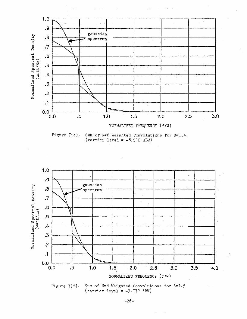
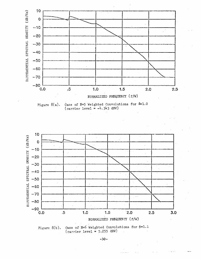
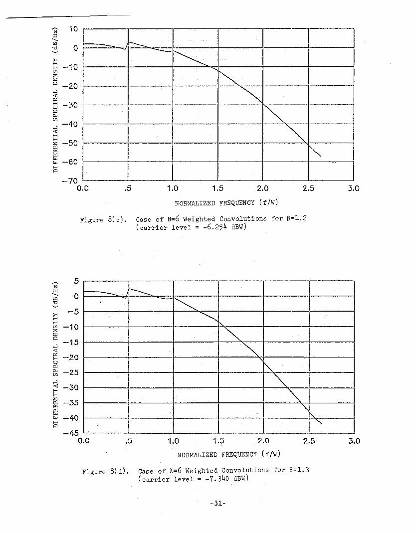
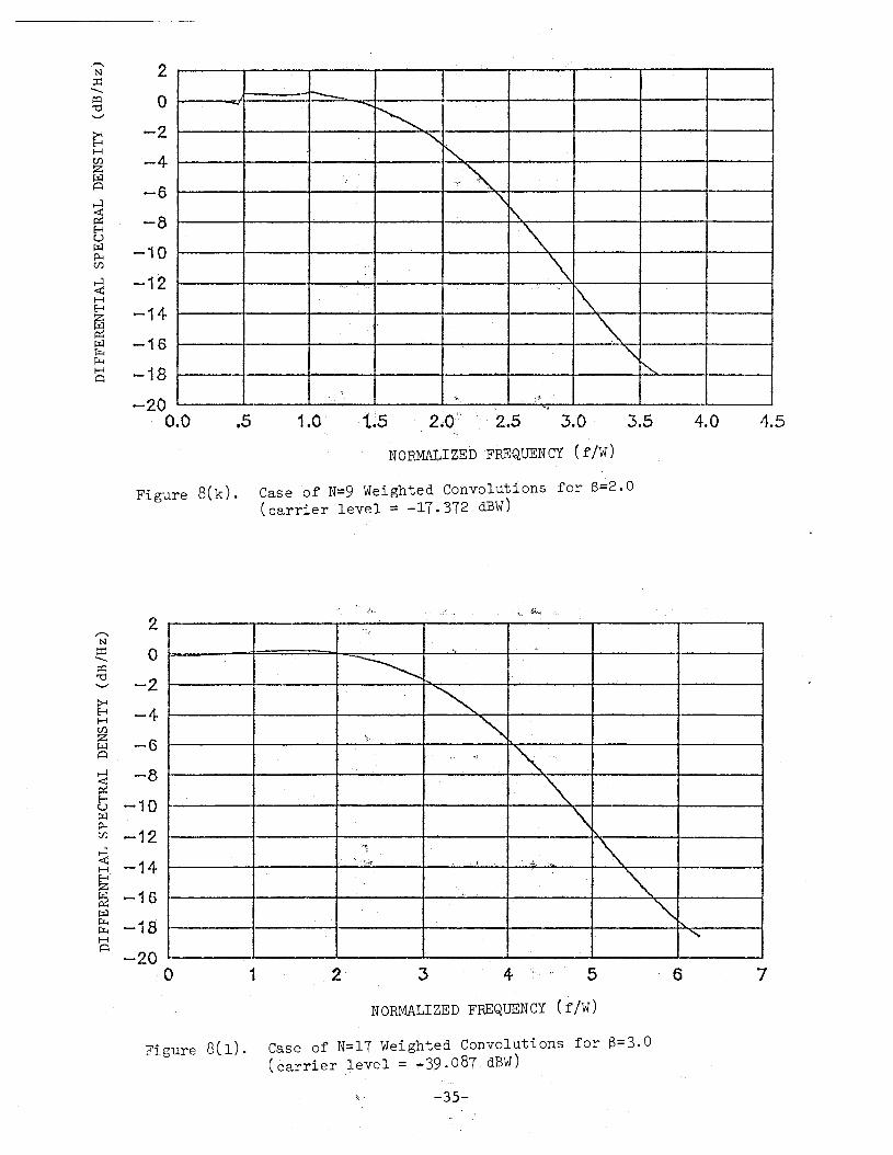
This e~presSion can. be compare~ tq the spectral convolution seriessimulation by setting W==l. The comparison resul~s are presented ,in Figures 7(a)to 7( 1), which show tha't thegau$sianapproximation is still poor at S = 1 buthas become effective beforeS, =:,,'2 is reached'. The cor:r~sponding db differentialbetween each pair is also presented in Figures 8(a) to 8(1), where the plots show10 log (Yl/Y2) with (Y1) as the gaussian spectrum approximation and (Y2) as thespectral convolution series • Hence " a negative dB ,differential in chese plotsimplies that the series spectrum exceeds the gaussian spectrum by that amount.

-23-

1.4

~ 1.2~.~

(J)

~<JJ 1.0~

r-f(1j

J-4""""~ N .8upj<JJ ...........p..~

CJ)~(1j

.6ro )<JJ'-"N.~

r-f(1j .4sJ-40z

.2

0.00.0 .5 1.0 1.5 2.0 "2.5

NORMALIZED FREQUENCY (f /W)

Figure 7(a). Sum of N=S Weighted Convolutions for 8=1.0(carrier level = -4.343 dBW)

f'-

\\.- gaussian

.. spectrum

r----\~

\~~

1.4

~ 1.2~.~

(J)

~ 1.0<JJ~

r-f(1j

~"""" .8~·N

up::<JJ ...........o..~CJ)~

.6(1jro )<JJ'-"N

.r-tH .4euSJ-40z

.2

0.00.0 .5 1.0 1.5 2.0

NORMALIZED FREQUENCY (f/W)

2.5 3.0

Figure 7(b). Sum ofN=6 Weighted Convolutions for 6~1.1

(carrier level = -5.255 dBW)-24-

~\~ gaussian

'\ speetrum

N~

~~~

1.2

~+JeM 1.0CI)

s::(1)~

M.8Cd,...,......

+J NCJ~(1) ............o..+Jtf.)+J .6Cd"C ~(1),-"N

eMM

.4Cds,...0z

.2

0.00.0 .5 1.0 1.5 2.0 2.5 3.0

NORMALIZED FREQUENCY (f/W)

Figure 7( c). Sum ofN=5 'Weig1)ted Convolutions for 6=1.2(carrier level = -6.254 dEW)

"

~

\- gaussian

'~-~', spe~ctru1n

N~

~

: ~\ ,f

1

X~

1.2

~1.0

oI-JeMCI)

s::(1) .80

,....eu~'"'

+J N .6CJ::o(1) .........o..oI-J

C/)oI-JCd

"0 :3.4w'-"

Ne..-f,....CdS~ .20z

0.0'0.0 .5, 1.0 1.5 2.0 2.5 3.0

NORMALIZEDFREQUEN CY (f!W)

Figure 7(d). ~ Sum ofN=6 'Weighted.Convolutions for e=1.3(carrier level = -7.340 dBW)

-25-

'"\ gaqssian

\.-~ spectrum

'"~~

i\

\"'\

",~

1.0

.9~

.8+JeM(/)

~ .7Q)~

r-f .6Cd~~+J Nu::r:: .5Q)""""o..+JCJ)+J

Cd .4~ :3Q),-,N

eM .3r-fCds

.2~0z

.1

0.00.0 .5 1.0 1.5 2.0 2.5 3.0

NORMALIZED FREQUENCY (f/W)

Figure 7(e). Sum of N=6 Weighted Convolutions for 8=1.4(carrier level = -8.512 dBW)

" \I

gaussian

",\..,-~ spectrum

~~

\,\

...-...._-~'\

"~

1.0

.9~+J .8eM(/)

~

.7Q)~

r-fCd .6,...~

+J Nu::r:: .5Q) ..........p..+J

CJ)+JCd .4~ ~

Q)'-'N

eM .3r-fCdS,... .20z

.1

0.00.0 .5 1.0 1.5 2.0 2.5 3.0 3.5 4.0

NORMALIZED FREQUENCY (r/w)

Figure 7(f). SumofN=8 Weighted Convolutions for 8=1.5(carrier level = -9.772 dBW)

-26-

'""'\ gallssian----"'- spE~ctrum

~

~

~\ i

~~._.,

'~

.9

>-. .8+J-,-4en .7~(1)~

r-I .6Cd,...,,-..+J N

.5tJ~(1)"",,-o..+Jtn+J

Cd .4"tj ~(1),-"N

-,-4 .3r-ICdS,...,

.20z

.1

0.00.0 .5 1.5 2.0 2.5 3.0

NORMALIZED FREQUENCY (f/W)

31.5 4.0

Figure 7(g). Sum of N=8 Weighted Convolutions for B=~.6(carrier level =-11.118 dBW)

~

K\~gaussian

~spectrum

."\~I~

~\ :."," i,

.~~

.5 1.0 t·~5 2.0 2.53.0

NORMALIZED FREQUENCY (r/w)

3.5 4.0

Figure 7(h). Sum ofN=8 Weighted Convolutions for 6=1.7(carrier level = ~12.551dBW)

-27-

~

'\\

\\ gaussian~spectrum

~.

'\\\~~

.8

~ .7~-rotenc:: .6QJ~

r-ftU .5~~~ N'CJ::cQJ ...........

.4p..a.JCJ)~

ctSP(j ~QJ'-' .3N.,..

r-ftUe .2~0z

•.1

0.00.0 .5 1.0 1.5 2.0 2.5 3.0 3.5 4.0 4.5

NORMALIZED FREQUENCY (f/W)

Figure 7(i). Sum of N=9 Weighted Convolutions for"S=1.8(ca-rrier level = -14.071 dBW)

~

\\l~gaussian

....----- spectrum

~,'.

"I

'\\L.~

~ >

0.00.0 .5 1.0 1.5 2.0 2.5 3.5 4.0 4.5

NORMALIZED FREQUENCY (r/w)

Figure 7( j ) . SUIIl of N==9 Weighted Convolutions for 8=1.9(carrier level = -15.678 dBW)

-.28-

".,' ..... ...,".. 'k ,"

i'\ I', ",' : <",

\ i

,~,"

,~\ gaussian"", spEac trulll

\ I

I

:r ,~

~~'"

.7

.1

0.00.0 .5 1.0 2.0 2.5 3.0 3.5 4.0 4.5

NORMALIZED FREQUENCY ( f/W)

Figure 7(k). Sum of 1~=9Weighted Convolutions for 8=2.0(carrier level = -17.372 dBW)

.:

~

\\\\ gaussian'Vspectrum

\." \

\ "

"~

.50

.45

.40

.35

.30

.25

.20

.15

.10

.05""

0.00o .1 2 4 5: 6 7 8 9

, NoRMALIZED FREQUENCY (r/w)

Figure 7( 1). Sum 6f"N=I7 'Weighted Cor(volutions for 8=3.0(c,arrier level = '-39. 087a:BW)

-29-

,..--- .. --l- ------......-.. J~

--.;J

~~

~~

"- --~

" "-~

~ 10N::c

--.......~ 0'"d'-"

~ -10HenZ -20~A

~ -30Hu~ -40~en

H -50<HHz -60~~~~~ -70HA

-800.0 .5 1.0 1.5 2.0 2.5

NORMALIZED FREQUENCY (r/w)

Figure B( a). Case of N=5 Weighted Convolutions for 8=1. 0(carrie'r level·: -4.343dBW)

_.I...-...... ----- J~...,.

~

~~

'-.

~~",.

~'\.'"

~ 10N

::c--....... 0~"'d'-"

~-10

H-20en

ZJ:x.lA -30

~ -4-0Hu~~ -50en

H< -60HHz

-70~~~ -80~

HQ

-900.0 .5 1.0 1.5 2.0

NORMALIZED FREQUENCY (flw)

2.5 3.0

Figure B(b). Case of N=6 Weighted Convolutions for S=l.l(carrier level = 5.255 dBW)

...30-

~ 10N~

...........J:Q

0'"(j'-'

~ -10HCf.)

Z~c:::l -20~

~E-t -30u~~Cf.)

~-40

HE-t -50z~~~ -60~Hc:::l

-- [ '-'---"---

----=---.Jr--....., '-~"

i~"'-

K~

.-. ~~~

-700.0 .5 1.0 1.5 2.0 2.5 3.0

NORMALIZED FREQUENCY (r/w)

Figure 8(c). Case of N=6 Weighted Convolutions for 6=1.2(carrier level = -6.254 dEW)

~ I~~~.

~ ..::-.........: ..

~~

'"~~

'\~

"""""~

"

~ 5N

::c........... 0~'"(j""-'

~:-5

HCf.) -10z~c:::l

-15~

~ -20E-tu~~ -25Cf.)

~ -30HE-tz

-35~~

-4-0~Hc:::l

-450.0 .5 1.0 1.5 2.0 2.5 3.0

NORMALIZED FREQUENCY (f /W)

Figure 8(d). Case of- N=6Weighted Convolutions for (3=1.3(ca.rrier level = -7.340 dBW)

-31-

--~~

R_.

~K

~. '"~

.~,,~

5

~ -5E-!HU)

gj -10A

~ -15~u~

~ -20U)

-25

-30

-350.0 .5 1.0 1.5 2.0 2.5 3.0

NORMALIZED FREQUENCY (f/W)

Figure 8(e). Case of N=6 Weighted Convolutions for 6=1.4(carrier level ~ -8.5l2 dBW)

- r----.

~

~""~

". ~

~ -

""~.

~ 10N

::r:"'"""~"'C 0'-'

~H -10U)

z~A

~ -20~~u~ -30~U)

~<t:

-40H~Z~~~ -50~~HA

-600.0 .5 1.0 1.5 2.0 2.5 3.0

NORMALIZED FREQUENCY (f/W)

3.5 4.0

Figure 8(r). Case of N=8 Weighted Convolutions for B=1.5(carrier level = -9.772 dBW)

-32-

- 1:----"-'

~~

~~

""'""""~'"'"

,,-.. 5N::c:

..........~ 0"'d'-"

~ -5Hen

-10z~~

~-15

~ -20u~P-len -25H<H -30E-tz~

~ -35~~~

H -400

-450.0 .5 1.5 2.0 2.5 3.0 3.5 4.0

NORMALIZED FREQUENCY (r!w)

Figure 8( g). Case of N=8 Weighted Convolutions for (3=1.6(carrier 'level = -ll.118 dEW)

~- ~

~I "I '"~

~

'"~~

,,-.. 5N

::c............

~ 0"'d'-"

~ ~5HenZ~0 -10H

~ -15Hu~~Cf) -20~HH -25z~~~ -30~

H0

-350.0' .5 1.0 1.5 2.0 2.5 3.0 3.5 4.0

Figure 8(b).

NORMALIZED FREQUENCY (r!w)

Case of N=8 W~ighted Convolutions for 8=1.7(carrier level = -12.551dBW)

-33-

~

~

~

~~

"~'"""~

5

-5~H

~ -10~~

H -15~~ -20.~

~

CJ) -25~H

~ -30~~ -35~

H

~ -400.0 .5 1.0 1.5 2.0 2.5 3.0 3.5 4.0 4.5

NORMALIZED FREQUENCY (f/W)

Figure 8(i). Case of N=9 Weighted Convolutions for f3=1.8(carrier level = -l4.071 dEW)

-. --......

~'"~

~'\

",

'"".......

"...... 5N~

"~0"'d

'-'

~H -5CJ)

z~~

H -10~E-!U~ =-15~CJ)

~~'-20H

E-!Zga~ -25~~

H~

-300.0 .5 1.0 1.5 2.0 2.5 3.03.5

NORMALIZED FREQUENCY ( f/W)

4.0 4.5

Figure 8( j ) . Case of N=~Weighted Convolutions for a=1.9(carrier level::: -15.678 dBW)

-34-

4.54.03.53.02.52.O:~:t~51.0•5

",

l- -----., -........ .~

"~.~

":..' ~

"\.';.,1 ~- '\.

'\~

''i'., ,,)'

";".', ,~./"i;.;

2

o-2

-4

-6

-8

-10

-12

-14

-16

-18

-200.0

NORMALIZED FREQUENCY (r/w)

Figure 8(k). Case of N=9 Weighted Gonvolutions for 8=2. 0(carrier level = -l7.~72 dBW)

2

o-2

-4

"'j,:

"~, ....

~

~.;~. ~

'" .:.

'""", ';'I),!" J I ,.;~, :'",,_ ~t, '""'.~,

1 2 3 4 5

NORMALIZED FREQUENCY (f/W)

6 7

Figure 8(1). Case ofN=17 Weighted Convolutions for 8=3.0(carrier level = -39.087 dBW)

-35-

SECTION 4

GENERALIZED ···FM SPECTRUM GENERATION PROGRAM

The rectangle ,c()nvolution .program results are limited to the basebandmodulation case considered. The existence of a wider variety of baseband spectraand preemphasis characteristics in practical applications motivates a moregeneralized FM spectrum simulation capability. The interest is to provide forbaseband spectral shaping and parametric assignmen't control by the user, and thecompromise is that a compact mathematical formulation of the spectral convolutionterms is no longer available. The computer program must now simulate the FMspectrum generation process itself, rather than implement available expressionsas done in the rectangle convolution program.

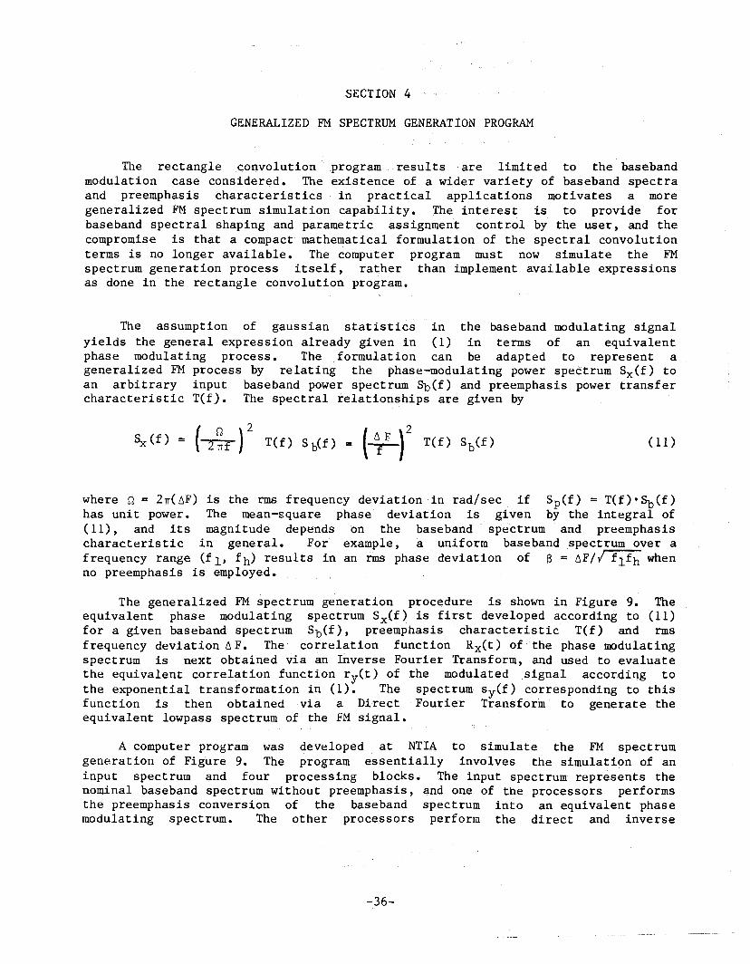
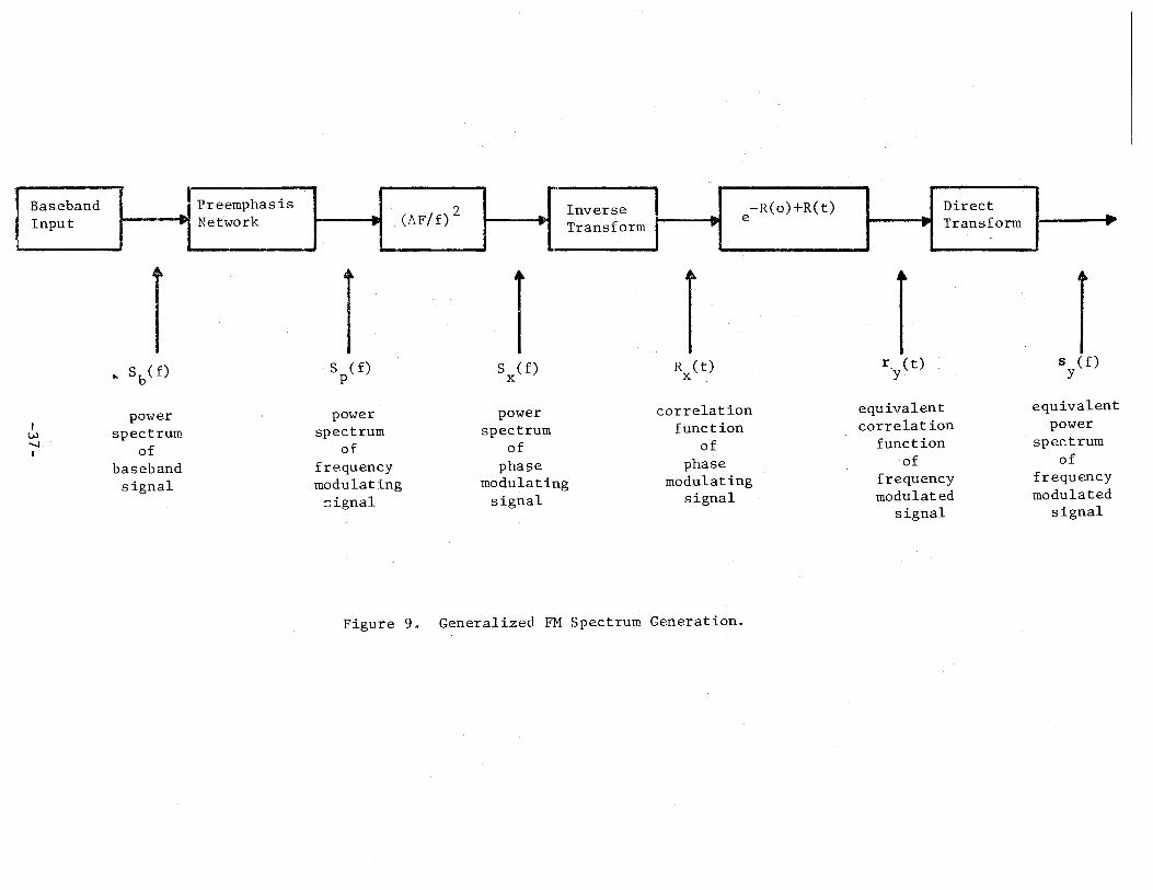
The assumption of gaussian statistics in the baseband modulating signalyields the general expression already given in (1) in terms of an equivalentphase modulating process. The formulation can be adapted to represent ageneralized FM process by relating the phase-modulating power spectrum Sx(f) toan arbitrary input baseband power spectrum Sb(f) and preemphasis power transfercharacteristic T(f). The spectral relationships are given by

(11)

where n = 27T(~F) is the rms frequency deviation'in'rad/sec if Sp(f) = T(f)· ~(f)has unit power. The mean-square phase deviation is given by the integral of(11), and its magnitude depends on the baseband spectrum and preemphasischaracteristic in general. For' example, a uniform baf)eband ,spectrum over afrequency range (f l' fh)' results in an rms phase deviation of f3 = ~FII f1fhwhenno preemphasis is employed.

The generalized FM spectrum generation procedure is shown in Figure 9. Theequivalent phase modulating spectrum Sx(f) is first developed according to (11)for a given baseband spectrum Sb(f), preetnphasis characteristic T(f) and rmsfrequency deviation ~ F. The correlation function Rx(t) of the phase modulatingspectrum is next obtained via an Inverse Fourier Transform, and used to evaluatethe equivalent correlation function ry(t) of the modulated signal according tothe exponential. transformation in (1). The spectrum sy(f) corresponding to thisfunction is then obtained via a Direct 'Fourier Ttan~form to generate theequivalent lowpass spectrum of the EM signal.

A computer program was developed at NTIA to simulate the FM spectrumgeneration of Figure 9. The program essentially involves the simulation of aninput spectruln and four processing blocks. The 'input spectrum represents thenominal baseband spectrum without preemphasis, and one of the processors performsthe preemphasis conversion of the baseband spectrum into an equivalent phasemodulating spectrum. The other processors perform the direct and inverse

-36-

IInverse -R(o) +R( t) Direct- e -, Transform I ... Transform .......

...

Baseband Preemphasis(~F/f) 2 ~

Inverse.... Network -..Input .. r po Transform

L· I ~.

~ Sb(f) S{f) S(f) R (t) 'r_ (t) s (f)p x x Y Y

power power power correlation equivalent equivalentI

VJ spectrum spectrum spectrum function correlation power'-J of of of of function spectrumI

baseband frequency phase phase of of

signal modulating modulating modulating frequency frequency

~ignal signal signal modulated modulatedsignal signal

Figure 9_ Generalized FM Spectrum Generation.

transforms involved, as well as the exponential transformation that simulates themodulation effect.

The continuous Fourier Transforms must be replaced by their discreteversions for computer implementation. This implies that a time-limited plusband-limited signal modeling is being provided, which represents a departure fromthe continuous case and requires careful accounting of distortion and aliasingeffects. A systematic procedure was developed to select the number of samplesfor an effective discrete representation in either time or frequency domain. Theprocedure can handle general unknown functions where only pulse width andbandwidth measures are provided, as well as typical test functions where specificparametric formulations are available.

A Fast Fourier Transform algorithm was employed for the Discrete FourierTransform realization. An existing in-house subroutine was analyzed and adaptedby the addition of a special purpose driver dedicated to deliver the inputsamples in a manner convenient for spectral analysis purposes. A menu of testsignals with their corresponding discrete formulations was developed to validatethe transform computation under various pertinent conditions (e.g., lowpass andbandpass spectra, finite or infinite pulse widths and bandwidths). Thetheoretical results were reproduced accurately in all cases, with only the idealretangular shapes requiring careful handling to accommodate the instantaneousdiscontinuity effects. The use of weighted mixtures of the test functions wasalso employed to simulate arbitrary spectral conditions and further validate thetransform algori~hms, by verifying that the mixture output corresponds to thewe:~ghted" supJer'position of the individual output results.

DISCRETE FOURIER TRANSFORMS

The Discrete Fourier Transform (DFT) consists of a direct and inversetransform pair employed to relate the discrete-time and discrete-frequency domainrepresentations of signal waveforms. The DFT provides for an accurateapproximation to the continuous Fourier Transform pair, and permits its practicalcomputation via digital computer algorithms. The Fast Fourier Transform (FFT)represents a modern efficient algorithm employed to compute the DFT.

A finite number (N) of samples is involved in the discrete time andfrequency representations of the DFT. This implies that a time-limited plusband-limited signal characterization is always provided. This represents adeparture from the continuous fourier transform, where a signal cannot be limitedin both the time and frequency domains simultaneously. The number of samplesemployed must be carefully selected to assure an adequate representation whensignals with an infinite domain in time or frequency are under consideration.

and

The direct and inverse DFT pair is specified by the formulas:N-l N-l nk

S(n) = t R(k) exp [-j (21T /N)nk] = r R(k) WN (direct)k=o K=O

-38-

(12a)

R(k) = 1N

N=l

1:n=o

8(n) exp [+j (2n/N) nk] = 1N

N=l8.(n)W -nkE N (inverse) (12b)

n=o

where R(k) represents the discrete-time samples, 8(n) represents thediscrete-frequency samples, and WN = exp [-j (2TI/N)] is noted to vary with thesample size (N). The same number of samples is employed in both the time andfrequency domain representations.

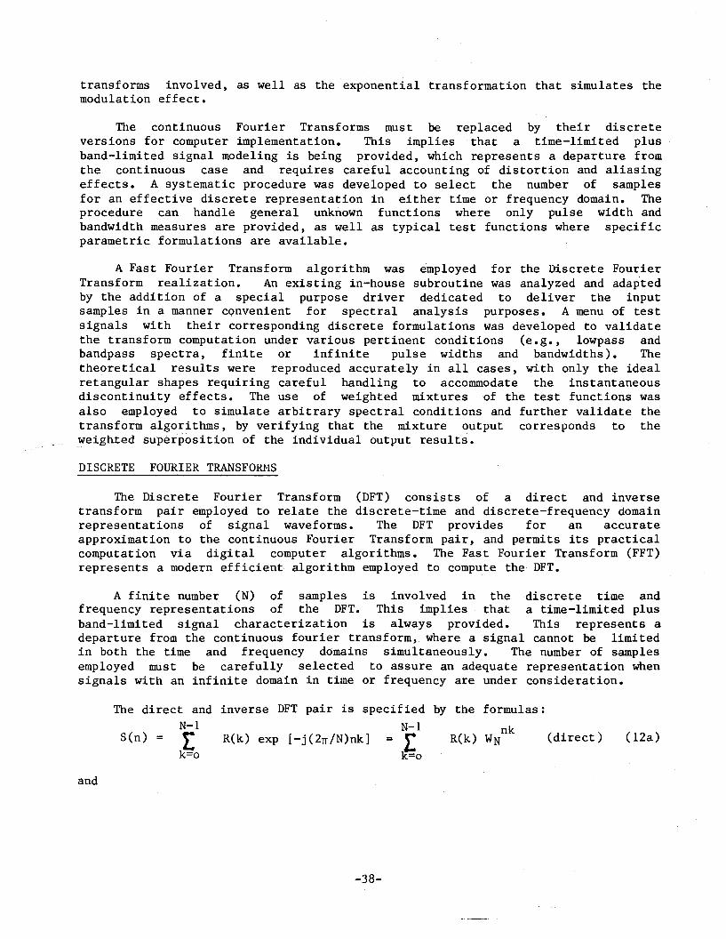
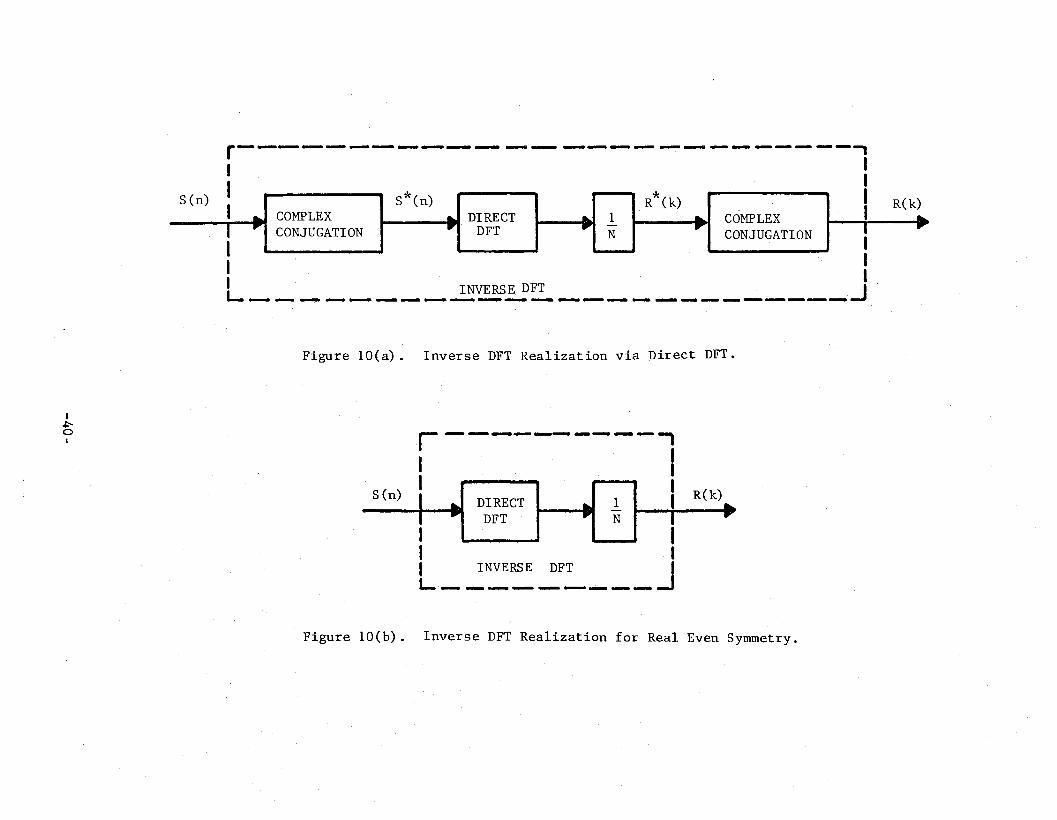
The time samples R(k) and the frequency samples Sen) can in general becomplex valued. The complex conjugate R*(k) of the time domain sequence can beverified to be identical to the direct OFT of the complex conjugate S*(n) of thefrequency domain sequence, except for the presence of a (liN) scaling factor.This permits the evaluation of the inverse DFT as a directDFT with simplemodifications as shown in Figure 10(a). The last conjugation can obviously beomitted for the case of real s~~ples in time. Moreover, a real even symmetry intime implies a real even symmetry in frequency, and then the inverse DFT reducesto a direct DFT with (liN) scaling as shown in Figure lOeb). This last case isof particular interest when evaluating autocorrelation and power spectral densityfunctions of real signals, since these functions exhibit a real even symmetryabout the origin in both time and frequency domains.

An inverse OFT is employed in Figure 9 to obtain the discrete correlationfunction Rx(k) from the di.screte power spectrum 8x(n). The latter represents thesamples from its continuous counterpart Sx(f), but the correlatioll values Rx(k)obtained via (12b) must be multiplied by N· ~f to represent sarnples from thecontinuous correlation function Rx(t). This effect is a consequence of theincremental spacings being implicit in the DFT summat'ion versus explicit in thecontinuous transform integr.al.

A similar effect occurs when using the direct DFT in Figure 9 to obtain theediscrete power ~~ectrum sy(n) from the discrete correlation function ry(k). Thelatter represents the sam,ples from its continuous counterpart ry(t), but thespectral values sy(n) obtained via (12a) must be divided by N·~f to representsamples from the continuous power spectrum sy(f). Notice that this division byN·~f does not cancel the above multiplication by N·~f since there is thenonlinear exponential transformation separating these effects in Figure 9.

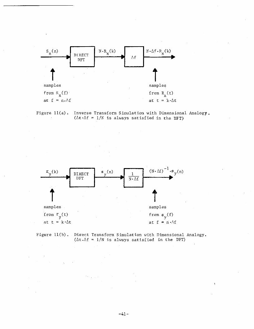
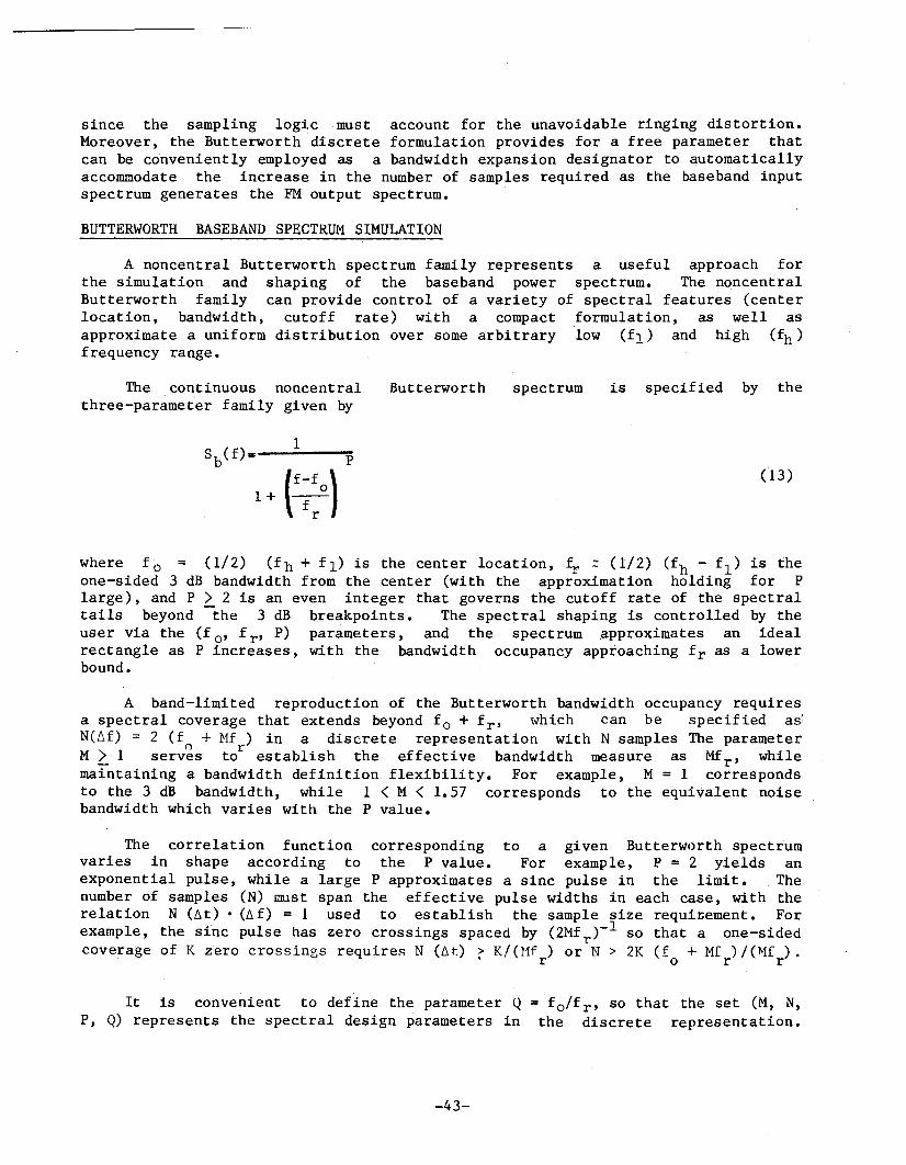
The inclusion of these scaling factors is 'necessary to maintai.'n dimensionalanalogy with the continuous signal representation. The net effect irlsofar as thesimulation logic is concerned is shown in Figures Il(a) and ll(b)., The inversecontinuous trarlsform is realized by a direct DFT plus a tJ.f multiplier, whichcorresponds to the inverse DFT with a N.~f multiplier. The direct continuoustransform is realized by a direct OFT with a N·~f divider, and the generation ofdBIHz spectral units only requires taking 10 log (e) of the DFT output data andsubtracting the constant 10 log (N·~f).

Nill1BER OF SAMPLES

The number of samples (N) employed in the DFT must be sufficient to providean effective representation of the continuous time and frequency functions

-39-

r--------·------------------,I I

II

I IIL .INVERSED:!._- .J

I S*(n) R*(k)S (n)I .... COMPLEX ... DIRECT .... 1 .... COMPLEXI .... -r DFT r - .,

CONJUGATION N CONJUGATIONI

Figure 10(a). Inverse DFT Realization via Direct DFT.

t,I::"­oI r -------------,

III .•.... . .. I

S(n) 1-1-. D.lREC.T I U]1:.. I R(k)DFT N I ..

I .... .... . .. ..... II IL_ ~NVE~ ~F:' J

Figure lOeb). Inverse DFT Realization for Real Even Symmetry.

S (n)x

tsamples

from S (f)x

at f = n.llf

DIRECTDFT

l~ItR (k)x

N·llf.R (k)x

samples

from R (t)x

at t = k·llt

Figure ll(a). Inverse Transform Simulation with Dimensional An,alogy.(~t ·llf =llN is always satisfied in the DFT)

r~ (k)y

samples

from r (t)y

at t = k·llt

DIRECTDFT

s (n)y

tsamples

from s (f)y

at f = ri·~f

Figure ll(b). Direct Tral1sform Simulation with Dimensional Analogy.(llt.~f, = l/N is always satisfied in th~ DFT)

-41-

involved. The fact that the same number of samples is used in both domainrepresentations implies that the selection rationale must jointly provide enoughtime spread and spectral occupancy to cover the effective pulse widths andbandwidths involved.

A standardized procedure was developed to log'ically select the number ofsamples (N), and is applicable'regardless of whether the direct or inverse llFT isbeing computed. The procedure can handle general unknown time or frequencyfunctions where pulse width or bandwidth measures are the only availableinformatioTh, as well as specific functions where detailed para"metric formulationsare assumed as models. In particular, the procedure was designed to handleeven-symmetric functions (autocorrelation~. power density) based on the immediateapplication of interest here.

Consider an even-symmetric input function wi,th a one-sided effective widthmeasure (Win). The input function will be assumed in the time domain forformulation purposes, without loss of generality since we only need tointerchange the time (t) and frequency (f) variables otherwise. The number ofinput samples (N) needed to cover the input with a uniform incremental spacing(~t) then satisfies N(~t) = 2 Win. The re'lation (~t) • (~f) = liN is inherent inthe DFT definition, and relates the input and output incremental spacings.Hence, a given number of samples (N) corresponds to input and output incrementsof ~t = 2Win/N and ~f = 1/2Win , and the net output width coverage capability isgiven by N(~t)/2 = 1/2Win (one-sided). This last amount must exceed the(one-sided) effective output width measure (Wout ), which yields the :requirementof N ~ 4 (Wen) (Wout ) for the sample number selection. Note this condition issymmetric In its joint accounting of the time and frequency domains (pulsewidths, bandwidths) as should be the case.

The selection of a baseband input spectrum is first used to establish alower bound on the number of samples required. An input bandwidth measure isavailable from the spectral shape, and the associated pulse width measure can beobtained from its corresponding correlation function. This minimum number ofsamples is obviously insufficient for the ultimate FM output spectrumrepresentation, since the bandwidth expansion effect must be accounted for. Thebandwidth expansion can be estimated using Carson's Rule or other FM bandwidthmeasure selected, and the corresponding increase in the number of samplesrequired becomes specified.

The baseband inp~t spectrum Sb(f) of Figure 9 was simulated to approximate arectangular shape with selectable low and high cutoff frequencies. A noncentralButterworth spectrum family was employed for this purpose, with the cutoff rate(spectral tail decay) carefully selected to assure that an effectiveapproximation to the ideal rectangle effects are preserved through the spectraltransformations of (11) leading to the equivalent phase modulating spectrum S (f)in Figure 9. x

The selection of a Butterworth spectrum instead of an ideal rectangle forsimulation purposes was motivated by practical DFT representation considerations.The step discontinuities of an ideal rectangle hinder a discrete simulation,

-42-

since the sampling logi.c must account for the unavoidable ringing distortion.Moreover, the Butterworth discrete formulation provides for a free parameter thatcan be co'nveniently emplo~red as a bandwidth expansion designator to automaticallyaccommodate the increase in the number of samples required as the baseband inputspectrum generates the FM output spectrum.

BUTTERWORTH BASEBAND SPECTRUM SIMULATION

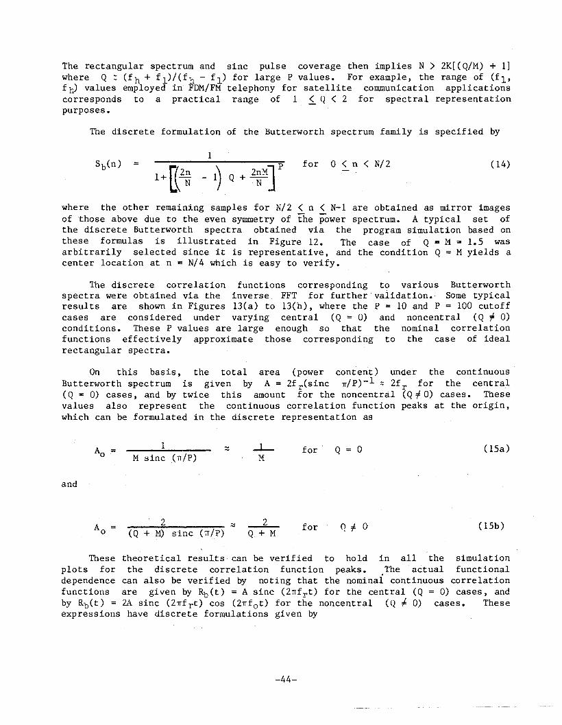
A noncentral Butterworth spectrum family represents a useful approach forthe simulation and shaping of the baseband power spectrum. The noncentralButterworth family can provide control of a variety of spectral features (centerlocation, bandwidth, cutoff rate) with a compact formulation, as well asapproximate a uniform distribution over some arbitrary low (f1) and high (fh )frequency range.

The continuous noncentralthree-parameter family given by

Butterworth spectrum is specified by the

1+

1p

(f~:o)(13)

where f o = (1/2) (fh + f1) is the center location, 4 :; (1/2) (fh - f 1 ) is theone-sided 3 dB bandwidth from the center (with the approximation holding for Plarge), and P > 2 is an even integer that governs the cutoff rate of the spectraltails beyond -the 3 dB breakpoints. The spectral shaping is controlled by theuser via the (f 0' f r' P) parameters, and the spectrum approximates an idealrectangle as P increases, with the bandwidth occupancy approaching f r as a lowerbound.

A band-limited reproduction of the Butterworth bandwidth occupancy requiresa spectral coverage that extends beyond f o + f r , which can be specified asf

N(~f) = 2 (f + Mf) in a discrete representation with N samples The parameterM > 1 serv~s tor establish the effective bandwidth measure as Mf r , whilemaintaining a bandwidth definition flexibility. For example, M = 1 correspondsto the 3 dB bandwidth, while 1 < M < 1.57 corresponds to the equivalent noisebandwidth which varies with the P value.

The correlation function corresponding to a given Butterworth spectrumvaries in shape according to the P value. For example, P = 2 yields anexponential pulse, while a large P approximates a sine pulse in the limit. Thenumber of samples (N) must span the effective pulse widths in each case, with therelation N (~t) • (~f) = 1 used to establish the sample size requi:r;ement. Forexample, the sinc pulse has zero crossings spaced by (2Mf r)-l so that a one-sidedcoverage of K zero crossings requires N (~t) > K!(Mf ) or N > 2K (f + Mf )/(Mf ).

'r 0 r r

It is convenient to define the parameter Q = fo/f r , so that the set (M, N,P, Q) represents the spectral design parameters in the discrete representation.

-43-

The rectangular spectrum and sinc pulse coverage then implies N > 2K[ (Q/11) + 1]where Q: (f h + f 1)/(f h - f 1) for large P values. For example, the range of (fl'fh) values employed in FDM/FM telephony for satellite communication applicationscorresponds to a practical range of 1 ~ Q < 2 for spectral representationpurposes.

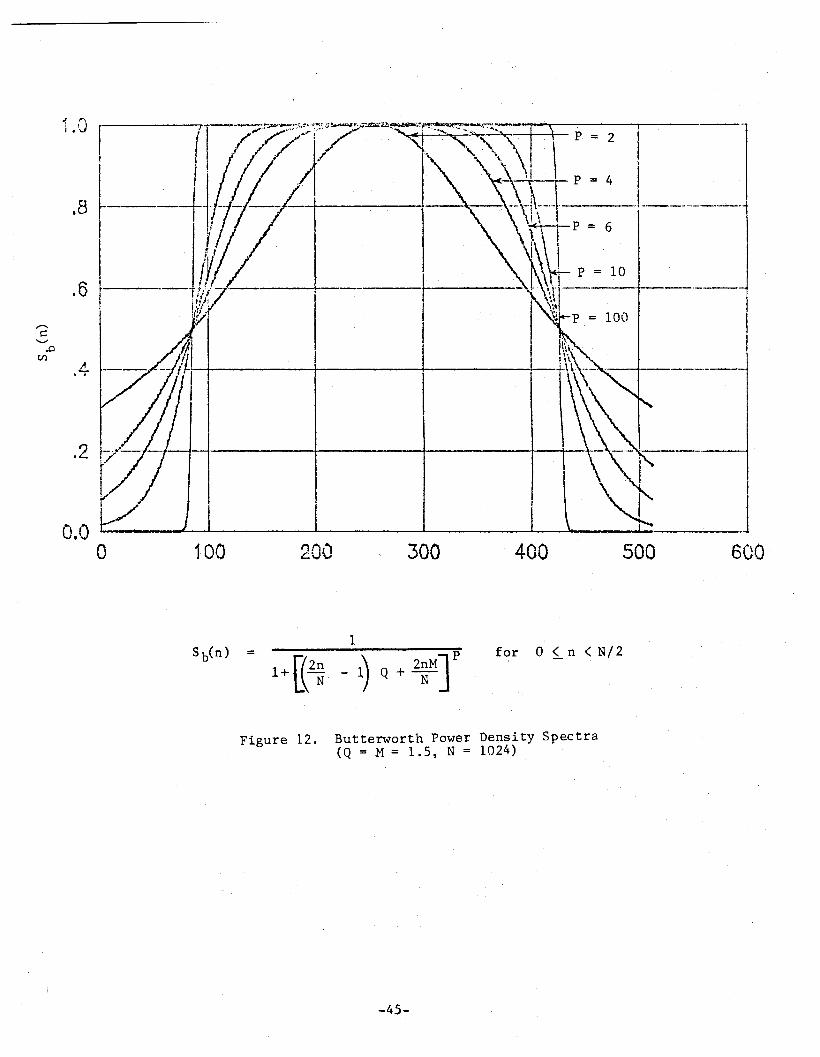
The discrete formulation of the But·terworth spectrum family is specified· by

1for 0 <n < N/2 ( 14)

where the other rema1nl.ng samples for N/2 < n < N-l are obtained as mirror imagesof those above due to the even symmetry of the Power spectrum. A typical set ofthe discrete Butterworth spectra obtained via the program simulation based onthese formulas is illustrated in Figure 12. The case of Q = M 1.5 wasarbitrarily selected since it is representative, and the condition Q = M yields acenter location at n = N/4 which is easy to verify.

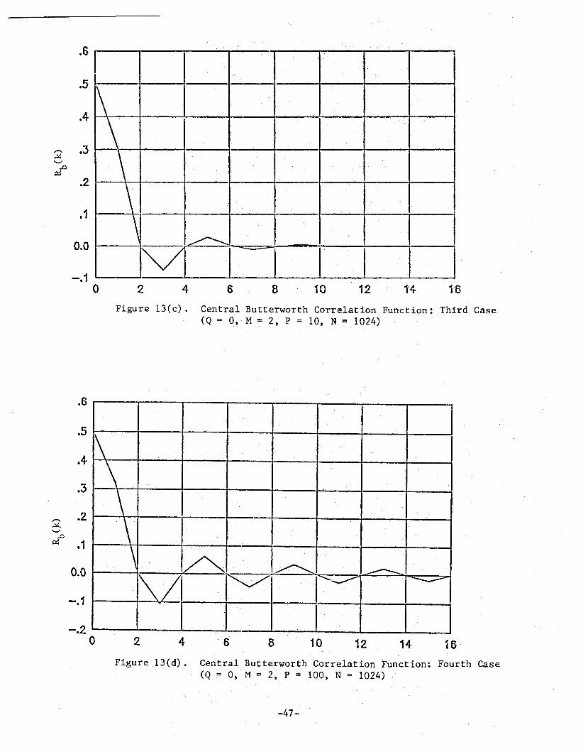
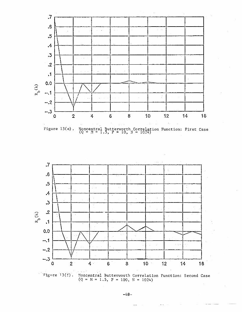
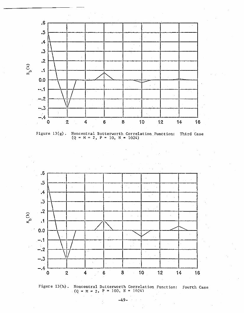
The discrete correlation functions corresponding to various Butterworthspectra were obtained via the inverse FFT for further validation.- Some typicalresults are shown in Figures 13(a) to 13(h), where the P = 10 and P = 100 cutoffcases are considered under varying central (Q = 0) and noncentral (Q ~ 0)conditions. These P values are large enough so that the nominal correlationfunctions effectively approximate those corresponding to the case of idealrectangular spectra.

On this basis, the total area (power content) under the continuousButterworth spectrum is given by A = 2f r (sinc 7T/p)-l z 2f r for the central(Q = 0) cases, and by twice this amount for the noncentral (Q:f 0) cases. Thesevalues also represent the continuous correlation function peaks at the origin,whieh can be formulated in the discrete representation as

and

A =o

1M sine (TIfp)

2(Q + M) sine ( nip)

2Q + M

for

for

Q o

Q f O'

(I5a)

(ISh)

These theoretical results can be verified to hold in all the simulationplots for the discrete correlation function peaks. .The actual functionaldependence can also be verified by noting that the nominal continuous correlationfunctions are given by Rb(t) = A sine (27Tf r t) for the central (Q = 0) cases, andby Rb(t) = 2A sine (2TIf r t) cos (2TIfot) for the noncentral (Q ~ 0) cases. Theseexpressions have discrete formulations given by

-44-

600500400300200100

n-~i('lJ:7~~~~S::\Ff P .~ 2 I·.··.. 1

y/ ... fi I P ~ 6

.6 ._-t({j --- ,. -S\\h1

o .~ ~ 10-+-- .'ld7~ \l~~\

l. 11 I ~ P ~ 100

·4 I-- --.- JI- ~._--_._-

1.0 I

.8~-

1=

1+[(2~ _l) Q + 2~M] P

forO ~ n <N/2

Figur4~ 12. Butterworth Power Density Spectra(Q = M = 1.5, N = 1024)

-45-

~

\\ .

\ -.

\\\ ~f"'-.

\j/ I ~I II

·7

.6

.5

.4

.3,........

.2~'-'

..c~

.1

0.0

-.1

--.2o 2 4 6 8 10 12 14 16

Figure 13(a). ,Cen.tral Butterworth Correlation Function: First:: Case.(Q=O, 1.1=1.5, P=10, N= 1024)

\

\\ -\ -

\ -\ I\ /K _~ I . -:---"'" ....----......- ----.\ I I Y ~ ........... ---

,~

~.

.7

.6

.5

.4

.3,........

.2~'-'

~.1

0.0

....1

-.2o 2 4 6 8 10 12 14 16

Figure 13(b). Central Butterworth Correlation Function: Second Case(Q = 0, M = 1.5, P = 100, N = 1024)

-46·~

.1 I10 12 1'4 1'6

.5

1

\

.4~\~~~~~~'

~.3 \

.2 J.-l~\~'J--~-+----------i--------t------t

.1 \. ~<··.I

:: ~~-~~~j~~~

02468

Figure 13(c). Central Butterworth Correlation Function: Third Case(Q = O,M = 2, P= 10, N= 1024)

.6 ,.....----r---..,..--'""---~......-.--..,.......-------,- __.........-----o....--..._--_.

'161412108642-.2 "----....A----...r.-.---~~ .._-L........------"-....I-__......._......L_------.....1. ___J

oFigure 13(d). Central Butterworth Correlation Function: Fourth Case

(Q= 0, M = 2~ P = 100,N ~ 1024)

-47-

·7

.6

.5

.4

•3

.2

.1

,......... 0.0~'-'"

,.c -.1~

-.2

~ I\\ .". ....

\ ..

\\ ~ I I\

1.-\-- /'\./y.----=m

I! -\1/

, r2 6 8 10 12 14 16

Figure 13( e) . Noncentral Butt'erworth Correlation Function: First Case(Q = M = 1.5,P = 10, N ~ 1024)

.7

.6

.5

A-...3

,......... .2~~

,.c.1~

0.0

....1

-.2

1\

\\

\ I\V

\1,/

161412108642

-.3 a.-~~...L-__.....................~~~_--..ll..- -""-__-",,__-,,

o

'Fig'llre J3(f). !'1oncentralButter~vorthCorrelation Function: Second Case(Q ~. M= 1.5, P = iOO, N = 1024)

-48-

1\

\\ ..

\\ / K --\ / ~~ I\ / --

1/ I2 4 6 8 1'0 12 14 16

Figure 13(g). Noncentral Butterworth Correlation Function: Third Case(Q = M ~ 2, P = lOJ N = 1024)

[\\

I.·· ·..1---\\ b~ I\ I / ~,

\ / I '"V

\ I/ ~\1/ I .

.6

.5

.4

.3

"'"".2

~'-'

..c .1~

" 0.0

-.,1

-.2

-.3

....4o 2 4 6 8 10 12 14 16

Figure 13(h). Noncentral Butterworth Correlation Function~ Fourth Case(Q = M= 2, P = 100. N = 1(24)

~49-

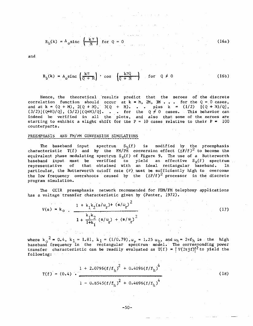
(16a)

and

(Q k7fQ

+ M ) for Q:/= 0 (16b)

Hence, the theoretical results predict that the zeroes of the discretecorrelation function should occur at k = M, 2M, 3M ~.~. for the, Q == O.cases,and at k = (Q +M),2(Q +M};'3(Q + M). plus k (1/2) [(Q + M)/Q],(3/2) [(Q+M)/Q], (5/2)[(Q+M)/Q]. for the Qf. 0 cases. .This behavior canindeed be verified in all the plots, and also that some of the.zeroes arestarting to exhibit a slight shift for the P = 10 cases relative to their P = 100counterparts.

PREE1~PHASIS ANDFM/PM CONVERSION SIMULATIONS:

The baseband input spectrum Sb(f) is modified by the preemphasischaracteristic T(f) and by the FM/PM conversion effect (~F/f)2 to become theequivalent phase modulating spectrum Sx(f) of Figure 9. The use of a Butterworthbaseband input must be verified to yield an effective Sx(f) spectrumrepresentative of that obtained with an ideal rectangular baseband. Inparticular, the Butterworth cutoff rate (P} falUSt be.. s,uffici.ently high to overcomethe low frequency overshoots caused by the (~F/f)2 processor in the discreteprogram simulation.

(17)V(s) = k o •

The CCIR preemphasis networkre~ontn;lendedfor.FDM/FM telephony, applicationshas a voltage transfer characteristic given by (Panter, 1972).

,,, . ··21 + k

1k

2(s/Wr )+ (s/wr )

where k o 2= 0.4,. kl = 1~81, kl = (l/O.79)~w = 1.2S.wh' and wh= 21Tfhis the highbaseband frequency, 'in the re'ctangular sp~ctrum·model.',: ThecorreRDonding powertransfer characteristic can be readily evalua!=edas T(f) ""IV(21TJnrito yield thefollowing:

1 + 2.0796(f/fh )2 + O.4096(f/fh )4T(f) -- (O;~ 4) . (l~)

1 - O.8545(f/fh

)2 + O.4096(f/fh

)4

-50-

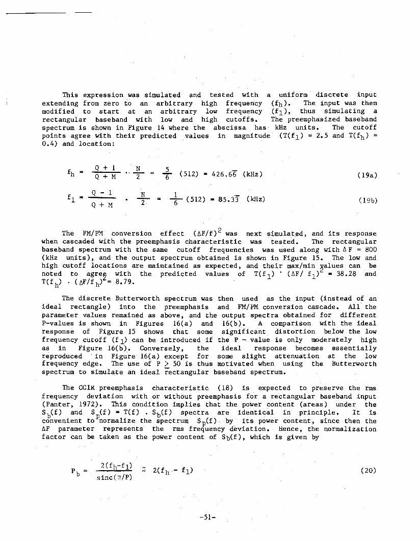
This expression was simulated and tested with a uniform d.iscrete inputextending from zero to an arbitrary high frequency (fh). The input was thenmodified to start at an arbitrary low frequency (f1)' thus simulating arectangular baseband wi.th low and high cutoffs. The preemphasized basebandspectrum is shown in Figure 14 where the abscissa has kHz units. The cutoffpoints agree with their predicted .values in magnitude (T(f1) = 2.5 and T(fh ) =0.4) and location:

fhQ + 1 N 5= ·'T = 6 (512) 426.66 (kHz) (19a)Q + M

Q - 1 :N + (512)f l = 2 85.33 (kHz) ( 19b)Q + M

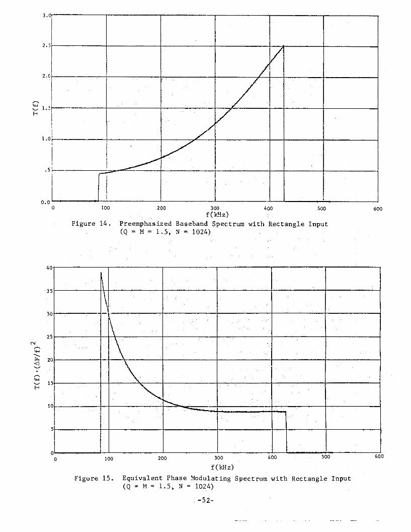
The FM/Pr.1 conversion effect (~F/f)2 was next s!mulat.ed, and its responsewhen cascaded with thepr,eemphasis characteristic was tested. The rectangularbaseband spectrum with the same cutoff frequencies was used along with ~ F = 800(kHz units), and the output spectrum obtained is shown in Figure 15. The low andhigh cutoff locations are maintained as expected, and their max/min ~alues can benoted to agre2 with the predicted valu~s of T(f 1) · (~F/ f 1 ) = 38.28 andT(f h) · (~F/fh)'= 8.79.

The discrete Butterworth spectrum was then used as the input (instead of anideal rectangle) into the preemphcisis and FM/PM conversion cascade. All" theparameter values remained as above, and the output spectra obtained for differentP-values is shown in Figures 16(a) and 16(b). A comparison with the idealresponse of Figure 15 shows that some significant distortion below the lowfrequency cutoff (f 1) can be introduced if the l? .... value is only moderately highas in Figure 16(b). Conversely, the ideal resp9nse becomes essentiallyreproduced 'in Figure 16(a) except' for some slight attenuation at the lowfrequency edge. The use of P > 50 is thus motivated when using th,e Butterworthspectrum to simulate an ideal ~ectangular baseband spectrum.

The Cell{ preemphasis characteristic (18) is, expected to preserve the rmsfrequency deviation witll or without preemp,hasisfor a rectangular baseband input(Panter, 1972). This condition implies that the power content (areas) under theSb(f) and Sp(f) = T(f) • Sb(f) spectra are identical in principle. It isconve,nient to normalizetllespectrum ,Sp(f) .by . t-ts power content, since then the6F parameter represents' the rms frequency deviation. Hence, the normalizationfactor can be taken as the power content of Sb(f), which is given by

2(fh- f l)

sinc(7fjp)

-51-

(20)

600200 300 400 500f(k:.tIz)

Preem.phasized Baseband Spectrum with'Rectangle Input(Q =M = 1.5, N=,1024)

Figure 14.

2. ~ r----'-----+-------....--+------~-_+_----~":__._+-~-__-~__+------~

3·°1

I2. 5i-' -------+-------+--------.+-------4---..-----4------~

'"' I~l.~r

I

1.0 1i---------+----.-----f----..,;c:--.--+--~------__+-_+__---___+_-----___fI

I.Sr-0.0 ~~......---......-_-...--------~I'-----------~-----..--......~_---..i

a 100

600500400200100 300

f(kHz)

Figure 15. Equivalent Phase Modulating Spectrum with Rectangle Input(Q = M = 1.5, N = 1024)

·

~

\"

'." ·

~\

,

·

\~ '" ;

~~ 'c, i

I

·

5

aa

30

10

40

25

-52-

600

100

500

50 arid P

400200100 300f(kHz)

Figure 16(a). Equivalent Phase Modulating Spectrum with PButterworth Inputs (Q = 'M = 1.5, N =' 1024)

~I P=100

I \~ -- P=50

\\\~~1

r

~i

II~

I 11)) ~ I

Joo

25

5

10

15

20

30

35

35

30P=lQ

25

C 20'-'~

CJ)

15

10

5

aa 100 200 300 400

f(kHz)

Figure 16(b). Equivale~nt Phase Modulating Spectrum with PButterworth Inputs (Q=·M = 1.5. N = 1024)

500

10 .1nd P 20

600

-53-

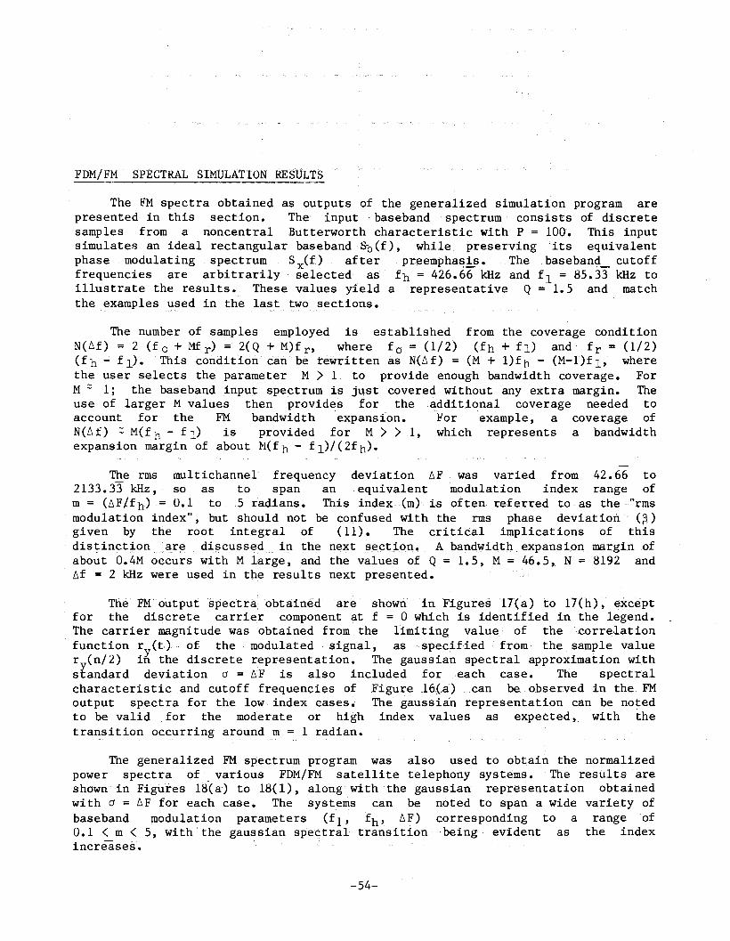
FDM/FM SPECTRAL SIMIJLATION RESULTS

The FM spectra obtained as outputs of the generalized simulation program arepresented in ,this secL'ion. Th'e input "baseb'and spec-trum 'consists of discretesamples from a noncentral Butterworth characteristicwit'h P = 100,. This inputsimulates an ideal rectangular baseband Sb(f), while, preserving its equivalentphase modulating spe,ctrum Sx(f.) after preempha~is. The baseband cutofffrequencies are arbitrarily selecte-d' as' fh= 426.66 kHz and f 1 = 85.33 kHz toillustrate the results. These values yield a representative Q ='1.5 and matchthe examples uS,ed in the la~c,t two sec~ions.

The number of samples employed is established from the coverage conditionN(~f) = 2 (f 0 + Mf r) = 2(Q + M)f r, where f o = (1/2) (fh + f1) and' f r = (1/2)(fh - f 1); Thiscondftidncari";' be rewritten as N(~f)= (M'-f l)fh- (M-l)f1' wherethe user selects the parameter M > 1 to provide enough bandwidth coverage. ForM z 1; th~ baseband input spect,rumis jq.st covered without any extra margin. Theuse of largerM values ~hen provides for the a'dditional coverage needed toaccount for the FM bandwidth expansion. For example, a coverage ofN(~f) :: M(fh - f1) is provided for M > > 1, which represents a bandwidthexpansion margin of about :tvl(fh - f1)/(2fh).

The rms multichannel frequency deviation ~F was varied from 42.66 to2133.33 kHz, so as to span an ,equivalent modulation index range ofm= (~Fifh')='0.1 to 5 radians. Thisindex·,,(m) is often" re,ferred to as the ;"rmsmodulation index", but should not be confused with the rms phase deviatidii,' (~)

given by the root integral of (11). The critical implications of thisdis~inc~~()n '. are d.;i.~cusse'd.,.. ;i.~ th~ next:~~ct~,q!!.. 1)., band.W'i4tb.,expan~iQnmarginofabout O.4M occurs with M l:arge, and the values of Q = 1.5, M = 46.5,: N' = 8192 and~f = 2 kHz were used in the results next presented.

;

The'FM"QutPl.it'spectta,6btB:ined 'are shown III Figures"'17'(a) to, 17{h) , exceptfor the discrete carrie,r component ~t f = a which is identified in the legend.The carrier magnitude was'obtained from the limiting value of the' '.correlationfunctionry(t) of the modulated signal, as spec1fiedfrom the sample valuer y (n/2) in the discre·te r\epresentat1,·on. The gaUSSian" spectral approximation wlthstandard deviation cr = ~F is also included for~ach case~ The spectralcnarCiC1:eristic ,and, c\ltofffrequencie,s of ,Figurf:.:16,(.a) ".can be. observed in.. the'FMoutput spectra for the lowinde:xea'ses. The' gaussian representation can be no~ed

to be valid ,for the moderate or high index values as expected, with thetransition occurring around m ~, 1 radian.

The generalized FM sp,ectrum program was also used to obtain the normalizedpower spectra of ,,' various FDM/FM satellite telephony systems. The results' areshown ,in Figures "18(a) to' 18(1) ,alongwith t'he" gaussian' representation obtainedwith cr = ~F for each case. The systems can be noted to span a wide variety ofbaseband modulation parameters (fl,fh , ~F) corresponding, to a range ,of0.1 ~m ~ 5, with I the gB:ussianspe·~t:ral transition being evident as the indexincreases.

-54-

~gaussian

".,---- spectrum,simulated

l"-t\. 7 rum

"y~

I~.. ' ,

\l

l.....- I \----..,;

\ ~

I~~

\ ~

. 1"-

-30~

N

~ -40~"t'-'-'

~ -50HCIlz -60~,~:

~:

~ -70~u~

~ -80Cf.),

~~

~ -90~

~-100oz

-110o 100 200 300 ~·oo 500 600 700 800 900

f(kHz)

Figure 17(a). FDM/FM Spectrum for m = 0.10(residual carrier ~ -0.157 dB)

~·I140012001000800400 '600

f(kHz)

Figure 17(b). FDM/FMSpectrum for rn = 0.33(~esidual carrier = ~1.749dB)

200

-55~

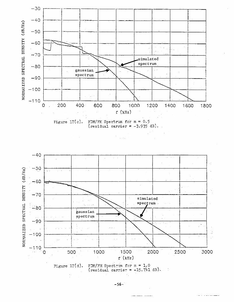
i

J

600400

--- ~~~-....---I----'---,'-'-'--',.~---t_---:---_i.---.;..---+-----__4

200

I~~____:_~~~~---....a-_----....-..i-~...........-.----..;,;;..;...;",;:.;,,-L--ao.- __- ------"'----.L-~_ __..J

800 1000 1200 1400 160'0 1800f (kHz)

--_. ----I----, ------, -----r------r------r------,.----..-_-30

"'"'""-40

N::r:

..........r=Q -5,Q,'"C'-'

~E-t '-60HCf.)

Z~~0

~70

~E-t

~80u~~Cf.)

~ -90,~NH

~ -1000z -110

0

Figure 17(c). FDM/FM Spectrum for m = 0.5(residual carrier = -3.935 dB).

3000

. I

25002000

simulatedspectrum

I

1000 150'0f" (kHz)

FDM/FM SpectrUm for m= 1.0Cresidu&l car:tier;: -15. 741 :dB) .',

. 500

Figure 17( d).

-40

",","", -50N::r:

..........~"'d'-'

~HCf.) "-70z~~

~ -=80'E-tu~~(J) -90Q~NH

-100~

~0z -110

0

-56-

-60,....N ~65::c

..........~

-70"0'-'

~ -75Htf.)

ffi -80~

~ -85E-tC,)~ -90~tf.)

~ -95~NH

~-100

0 -105z

"

--- -~ --.....-...

~i~

.'-

I ~ II ~

~!

~~~imulated Igaussian spectrum

spectrum -K'", ,'... I

"\ ~ II "\ ~~

"\ '"500 1000 1500 20002500 3000 3500 4000 4500 5000f (kHz)

Figure 17(e). FDM/FM Spectrum form = 2.0(residual carrier, = -62.964 dB).

1000 2000 30004000f (kHz)

5000 6000 '7000

Figure 17( r). FD:M/FM Spectrum for m = 3.0·(r,esidual carrier = -141. 669 dB).

-57-

~65:'

".......N ':;:'70-::r::

""""~"'d'-" -75~H

-80(J)

z~~

~-85

E-t-90u

~~(J)

~ -95J:;t:INH

-100

~0 -105z

-1100 1000 2000 3000 4000 5000 6000 7000 8000 9000

f (kHz)

Figure 17(g) . FDM/FM Spectrum fQr m = 4.0(residual carrier = -251.857 dB).

·2000 30f)O 40()O 5000 60007000 800b 9000

" f (kHz)Figure 17(h). FDM!FMSpectrum'f'or m':: 5.0

·(residual·····carrier· ,'< .... 390 . dB) ·

-58-

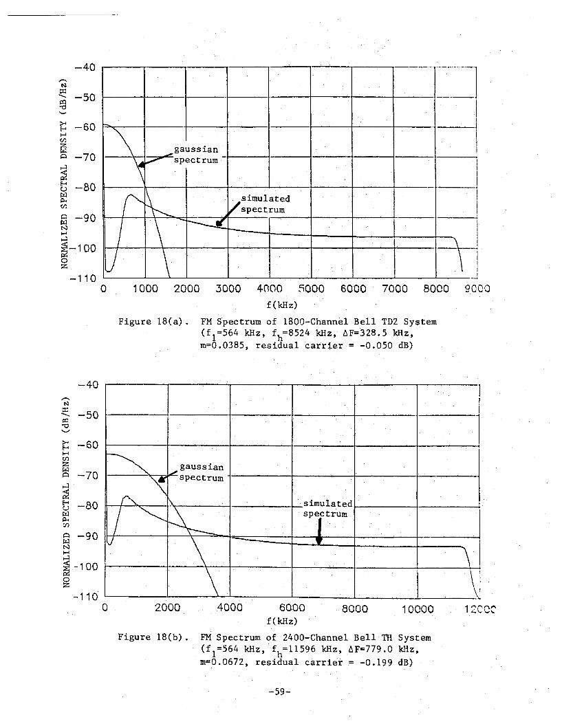
-40 ,--...;,..--- .-.--;..------~~~..._"""-------_._. -----_._---

+-------~- .....-- ----...--4

~ -60HCJ)

Z~

~~ -70

~.~ -80~P-4'CJ)

~ -90NH~

!-100oz

-110o

simulatedspectrum

1000 2000 3000 4000 ~OOO 6000 7000 8000 9000f(kHz)

Figure 18(a). FM S'pectrum of 1800-Channel Bell TD2 SystE~m

(f1 =564 kHz, fh

=8524 kHz, t.F=3·28.5 kHz,m=O.0385,residualcarrier = -0.050 dB)

1

j

1ZCOClOOO()8000.40002000 6000·f(kHz)

Figure 18(b). FM Spectrum of 2400-ChannelBell TIl Systenl(f

1==564 kHz, f

h=11596 kHz, !J.F=779.0 kHz,

Ill=O.0672, residual carrier=-O.199 dB)

".....N~ -50............~"'0~

~ ~60E-tHCJ)

Z~

-70~

~

~E-t -80u~P-4:I.l

-40

-59-

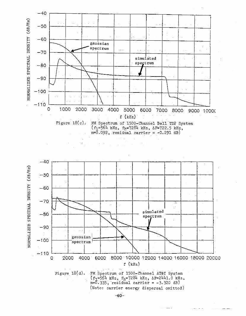
3:000 4000 5000 6000 7000 8000 9000 1aooe'; f(kHz)

FMSpectrum of1500-Channel Bell'"TD2 System(fl=564 kHz, fh=7284 kHz, ~F=722.5 kHz,m=O .09~, \re~idual ;carrier =-0.291 dB)

-40,-....N

::x::-50..........

~"tJ'-'

~ -60E-4HCJ)

Z~

-70A

~E-4 -80u~p...CJ)

0 -90~NH~

~ ·-1000z

-1100 1000 2000

.I

Figure 18( c) •

~110

o

-40

-50

-60

-70

~80

-90

~100gaussian 'Il_--Jl-------t--.~,

~--~~spectrum

2000 4000' 6000 8000 '1 0000 l2·000 14000 1'6000 18000 20000r{kHz)

Figur~h18(d) •• ,FM S:p~,ct.rum: of 1500:..Gh~nel AT&T System(hf5p4 .. fHz, t'h=7284 kHz. ,~F=2441. 0 kHz,m=O~335,'residual carrier = -3.320 dB)(Note: carrier energy dispersal omitted)

-60-

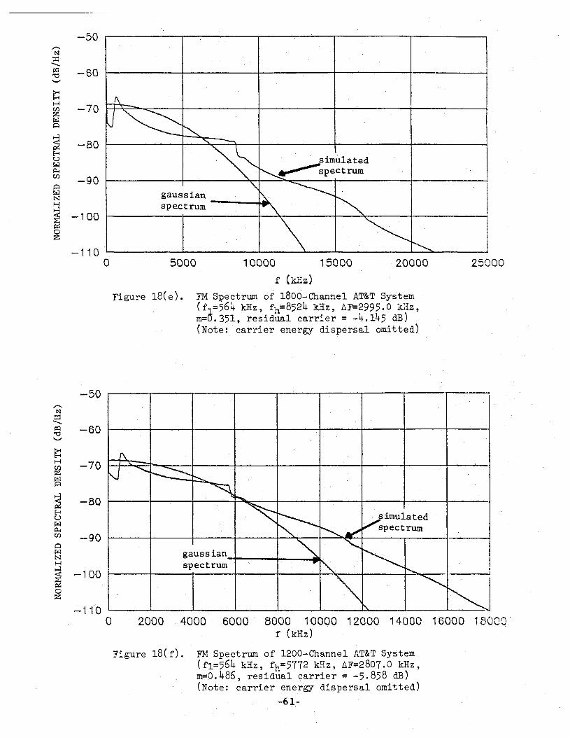
250002000015000

simulated~spectrum

10000

gaussi.snspectrum --~--~.

-50r".N

::c.........~ -60"0'-'

~H

-70tJ)

zI:i:t~

~ -80E-tuI:i:tP-4tJ)

-90~I::rJNH~

i -1000z

-1100

f (kHz)

Figure l8(e).. FM Spectrwnof laaO-Channel AT&T System(:£'1=564 kHz, fh=8524 kHz, t:.F=2995. 0 kHz,m=O.351, residual carrier = -4.145 dB)(Note: carrier energy dispersal omitted)

-50

-60

-80

-70

gaussial1....,..-----......------11...spe,ctrum

-90

~HU~P-4tJ)

~~NH

~ -100oz

2000 4000 6000 8000 10000 12000 14000 t6000 18000'f (kHz)

Figure l8(r). FM Spectrum of 1200-Channel AT&T 'System(f1=564 kHz,fh=5772 kHz,~F=2807.0 kHz,m=O.486, residual carrier = .... 5.858 dB)(Note;: carrier energy dispersal omitted)

-61·

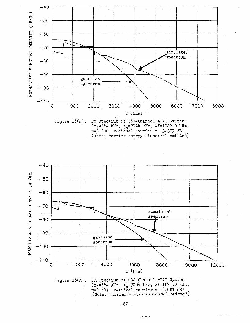
-40

-50

gaussian .....- .......---., •...spectrum

80007000Sooo20001000 3000" 4obof (kHz)

Figure l8( g) . FM S~ectrum of 360-Channel AT&T System(fl~56'4 kHz" fh=2044kHz,.~F=1022.0 kHz,m=O. 500, residual carrier = -3. 379 dB)(Note:car'r'ier energy-dispersal omitted)

1000060,00

f (kHz)

gauss ian'~.,f....---.............lI\".

spectr'um

'2000

Figure 18(h). FM Spectrumof:600-Channel AT&T System(fl =564 ,kHz', f h=3084 kHz', LiF=187l. 0 kHz,m=O.607,residualcarrier = -6.081 dB)(Note: carrier energy dispersal omitted)

-62-

.j

I,

80007000

~--+------_.

5000

_ ...._- _._-,·simulated .-.- .----,

spectrum...- ..~ . '_..- .__.--.4

I,

3000' 4000f(~-qz)

20001000

gaussian ................... ....11"1

-_. --------- -'- spectrum·-

..__... .i- ~__,.

--_ -..,_... . -.-_..... ..-,..-.---- -.. .~ -. ---'.~" - ,- --- __..---------- ----.- ~-. . -·--1.. _-- .._ -.~.- .'. --.-•..__ . - ,.. _ ~, ..,.,-..•~.~.-.'._----.,--_. -_.__ . _---_..

-~~~~_ ..__~_._._.-.-- ..~-- ~~-~~~--~._ .---"""'--"-.. -~ ... ~~.•. ~;-=_-=~~.~~···~-l

L.-.-__•.__

-60

-65

-70

-75

-80

-85

-90

--95

-100

-105

-110o

Figure 18( i). FM SpectrUtIl of 360-Channel Western Union System( f·=60. 'kHz, f .=1550 kHz,' LlF= 1250.0 kHz,m==~.806, resi&ual carrier == -36.108 dB)

-65"......N

::c -70...........~"'(j'-' -75~H

-80Cf)

z~~

~ -85~

.E-4 -90U~p..Cf)

-95~~NH -100~

~ -105'0z

-110 '0 1000 2000 3000 4000 5000 6000 7000 8000 9000

r(kHz)

Figure 18(j). FMSpectrumof 420-ChannelWestern Union System(f1=6okHz, fh=1796 kHz, ~F=1645.6 kHz,m=O. 916, . residualcarrier=> --55.200 dB)

-63-

.--------'----_. ---_.-,.-----.------- -----

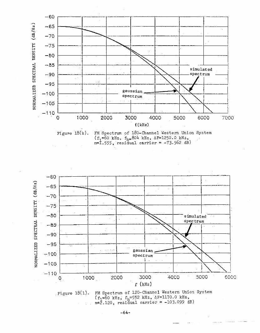
I

~Ii

---100----- ,_, ' .--__~

t----------. -----

gauss :ian _---t---.......---~spectrum

..-_---"-------- . --------_.._- ------_........_-- ._-----'--........---_.~----- .-.._--

1-----...... --,--'--t--------t-------+-~--""~~--

-"-' ,---,-,---1--.~

7000600050002000,1000 3000 4000f(kHz)

Figure l8(k). FM Spectrum of 180-Channel Western Union System(f1=60 kI~z, f p=804 kHz, . A.F=1250. 0 kHz,m=I.555~' residual carrier = ..73'. 562 dB)

EOOO50004000

'.--.----~------.------~

3000f (kHz)

2000

._---,---------...----------.--- .--------,.;...-------

1000

,......... ---..-..;,,;.-::-~--.- __._------4

');-_---- , ' --', ----.'' 'J---,---~---

-60,,-...N

::c: -65...........~"d

-70'-'

~, -75H(/)

Z~ -80A

~ -~85'HiU:~' -90~(/)

A -95~,

NH

~:~100

-1050z

-1 100

Figl).re· 18(1). FM Spectrum of 120-Channel Western Union System(fl =60 kHz, fh=552 kHz, ·~F=1170.0 kHz,m~2.120,res'idual carrier = -103.099 dB)

-64-

The normalized power spectra of· some of' theseFDM!FM systems hcive also beenpresented in a recent FCCdocu.ment (Sharp, to be pUblished). They were obtainedvia different simulation principles' and procedures than those used here, and theresul ts are included in Appendix: B for comparison purposes. The cases presentedhave the following counterparts in this report:

COMSTAll 360 corresponds to Figure 18(g)COMSTAR 600 corresponds to Figure 18(h)COMSTAR 1200 corresponds to Figure 18{f)TELSTAR 1800 corresponds .toFigure 18(e)WESTAR 120 corresponds to" Figure. 18(1)WESTAR 180 corresponds to Figure18(k)

The first four cases all represent low--index modulations, and there isnotable agreement with their counterparts in this report. The only distinctionappears in the low-frequency peak Defng slightly higlter in the FCC simulation,which is attributed to the higher peak inthepreemp'hasized baseband spectrumwhen using an ideal rectangle instead of a Butterworth baseband as previouslydiscussed. The last two cases represent higher-index~dulations, and there isagain general agreement between the two simulation results though the referencespectra are somewhat lower than their counterparts in this re~port. Thediscrepancies can be attri.b.uted to a higher spectrum arising from aliasingeffects in the NTIA model, or to a lower·spectrulD. arising from convolution seriestruncation in the FCC model. The distinction becomes academic, sinc.e the samegaussian spectral approxi'mation holds well and is to be used 1n thesehigher-index cases.

-65-

SECTION ,5

SUMMARY ••. AND· ···DISCUSSION OERES:ULT,S

The gaussian spectral approximation for high-index FM signals can bemotivated in two ways ,witha,gaussian'baseband modulat~on process of· arbitraryspectrum being always ass··umed. One approach reli,es, on Woodward's theorem, andidentifies the limiting spectrum 'to the statistical distribution of the frequencymodulating signal thus ind,Ucing the gaussian representatIon. The other approachuses Middleton's expansion. to ,.·develop a we:ighted superposition of spectralconvolution terms, which is maJlipulated into a gaussian approximation under highmodulation index conditions.

The ~tandard deviation (0), ,of the gaussian' spectral approximation representsthe rms bandwidth'of the modulated s,igpal,and:must be specified lnte-rms of themodulation parameters for the spectral representation., The fi'rst approach(Woodward.'s theorem) yields a = ~ F in terms of therms frequency deviation(~F),

while the second. approach· (Middleton's expansion)' yields· 0 ;:: s. Bx in terms of therms phase deviation (13) and the rms bandwidth (B x ) of the eqUivalent phasemodulating signal. These two formulas are not always ,'easily interchangeable,with the selection between them governed by the.capability to quantitativelyidentify the parameters involved in each case.

The inclusion of a preemphasisnetwork becomes :a critical consideration,since it can be designed to preserve the rms phase (13) or frequency' (~F)

deviation but not both in general (and perhaps neither in a given application).For example, an ideal preemphasis characteristic (parabolic power transfer) makesthe preemphasized FM baseband behave like aPM baseband so that 0 = I3.Bx becomesthe natural approach. Conversely, the CCIR preemphasis for FDM/FM telephonypreserves the rms frequency deviation and motivates using 0 = ~F to specify thegaussian spectrum parameter (Panter, 1972).

The rectangle convolution program was developed 'to analyze the gaussianspectral representation based on Middleton's expansion. The case of arectangular baseband spectrum (down to zero frequency) and ideal preemphasisyields compact iterative expressions for the spectral convolution terms, thusbypassing the need to actually simulate the multiple convolution operations.These expressions were logically programmed along with the weighting coefficientdistribution to generate the FM spectra as a function of the rms phase deviation(13). The number of spectral convolutions accounted is user selectable to provideany desired power preservation percentage. The results concluded that thegaussian spectral representation with 0 = B-Bx becomes effective beyond 13::::· 1.5radians for the baseband modulation under consideration.

The generalized FM spectrum program was developed to analyze the gaussianspectral approximation based on Woodward's theorem. A rectangular basebandspectrum with low (£1) and high (fh ) cutoffs was simulated via a noncentralButterworth family that provides user selection of the location frequencies andcutoff rates, plus a spectral coverage parameter that accommodates the FMbandwidth expansion and controls the discrete representation aliasing. The

-66-

program again bypasses the multiple convolutions simulation by exploitingcorrelation function dependencE~sand in~luding discrete spectral transforms asneeded. The gaussian representation with a' =~F was found to be become effectivebeyond m = 6. F/f h Z o. 7 :in both controlled parameter tests and existing systemssimulations.

The normalized carrier component is always given by -e2< 10 log e) dB, interms of the rms phase deviation (S), so that the latter must be specified for acompact formulation (except for the~a values where the carrier component becomeSnegligible). The rectangular baseballd sp'ectrum with low and high cutoffs yieldsa= ml v'Ewithout preemphasis, where' t = f1/f h < 1 so that a )In always. The

CCIR preemphasls case does not yield an exact compact result, but an effectivefunctional approximation to the preemphasis characteristic has been used todevelop the approximate relation (CClR~ ~978);

O.63m

1£(1-£)[1+2 .89e:'-3.17c2"0. 72£4] 1/2 (21)

A comparison between the normalized carrier component de'rived from this lastexpression and those obtained via the generalized FM simulation program ispresented in TABLE 2. There is close agreement between the two results in allcases, including the 18(g) case where a large (m)relative to 18(e) or 18(f) isnot accompanied by a larger (8)aIld the. carrier magpltudesincrease accordinglyin both results. The f'unctional approximation to the preemphasis characteristi~

was also compared to the actual characteristic (18) and found to overlap evenunder extreme (f l' f 'h) conditions represen~ati.ve of existing systemspecifications.

The ratio elm' obtained from (21) represents the conversion factor needed todetermine the rms phase deviation (8) from the indexm = tJ.F/fh. This convers,ionfactor is shown in Figure 19 as a function ofe:= fl/fh • The paraIneter E: spans,the range of 0.001 < £ < 0.275 in eXisting system specifications, whichcorresponds to a range-of --20 ) aim> 1.75 for the conversion factor. The latterremains around 8 Im'~ 2 for € > O. T, butincreasessignificarttly for € < 0.05 asshown, in the figure.

The conversion factor elm can be used to directly formulate the residualcarrier component via -S2(lO log e) dB, instead of deriving it from thecorrelation function measurement. The formula approach is preferable since the'extreme baseband cases (£«1) can introduce a simulation compromise betweenincremental resolution (fj,£ small) and aliasing control (N·6.f lar'ge} that canaffect the carrier measu:rement accuracy. The gerteralizedspectrum, prog'ram hasnow been modified to compute the carrier magnitude directly from the rms phasedeviation (f3), after such parameter is computed via (21) from the input ba$ebandcutoffs (£1' fh) and the rms frequency deviation (liF).

The following procedure has now been implemented to generate the FM spectrumfor given modulation parameters (f1 , f h , 6. F). The values of m ,- F/fh and'

£ = f Ilf h are first computed to obtain the nus phase deviation (8) from the

-67-

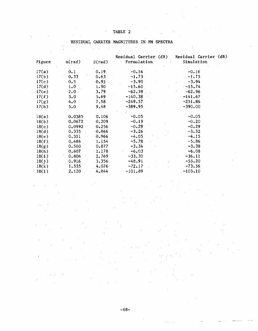
Figure

17(a)17(b)17(c)17(d)17(e)17(f)17(g)17(h)

18(a)18(b)18(c)1~(d)

18(e)18(f)18(g)18(h)18(i)18(j)18(k)18(1)

'RESIDUAL eAJmIER MJ\GNITUDES IN 'FM SPECTRA

Residual Carrier (dB) Residual Carrier (dB)m(rad ) S(rad) Formulation .' Simulation

0.1 0.19 -0.16 ....0.160.33 0.63 ~1.73 -1.750.5 0.95 -3.90 -3.941.0 1.90 -15.60 -15.742.0 3.79 -62.39 -62.963.0' 5.69 --140.38 -141.674.0 7.58 -249.57 -251.865.0 9.48 ";'389.95 -390.00

0.0385 0.106 -0.05 -0.050.0672 0.209 -0.19 -0.200.0992 0.256 -0.29 -0.290.335 0.866 ....3.26 -3.320.351 0.966 -4.05 ~4.15

0.486 1.154 -5.78 -5-.860.500 0.877 -3.34 -3.380.607 1.178 -6.03 -6.080.806 2.769 -33,.30 -36.110.916 3.356 -48.91 -55.201.555 4.076 -72.17 -73.562.120 4.844 -101.89 -103.10

-68-

20

18

16

14.

12

s 10·"'-en.

8

6

4

2

\\\~~~

o0.00 ..05 .10 .15, .20 .25 .30

e::=f1/fh

£: J.~ e:: S/m0.001 19.961 0 .. '10 2.3550.005 8.996 0.15 2,,3550.010 6 .. 422 0.20 1.8970.050 3.082 0.25 1.795

Figure 19. Conversion Factor (S/m) as a Functionof Baseband Parameter (e::)

-69-

expression (21). If S>1.5 (or any other bound selected) , the gaussian spectralapproximation with a =~ F is used to generate the continuous portion of thespectrum. If S<1.5, th~n~he generaliz;,ed ,spectrum program is used to generatethe continuous portion of the spectrum. In either case, the residual carriercomponent is gene~rat.e4 .. a§ ,~S2(lOlog ,e) ,from the"rms, phasedeviatio'n (S) alreadycomputed.

The generalized spectrum simulation program is now operational and automatedto deliver the FDM/FM system spectra from' a set of equivalent modulation inputparameters selected by the user. The program first decides on the gaussianspectral.approximat.ionvalidity, computes the gaussian:standarddeviation if suchapproximation is indeed valid, and ge,nerates the appropriate gaussian spectrumsamples. Otherwise, theprogram"'negates thegsussi'atf spectralrep'resentation andprocee,ds to deliver the proper spectral samples as generated by the generalizedFM simulation··process.

The ..·FDM/FM .simulation pr-ogramrta's alsobeeri.·~'iDatchtidto drive another existinginterference analysis program for FDM/~~M telephony. The interference programcomputes the output NPR pet' telephony 'channel" 'for' a given ~DMIFM input spectrumas the desired signal and a given arbitra.ry interferen'c~,spectr9mselected by theuser. The, FDM/FM simulation program repo~ted here provides for the desiredsignal spectrum, and a set of interference ~pectrCll simulations are beingdeveloped to supplement those alrea;4Y aval1ablefrom the interference programmenu.

-70-

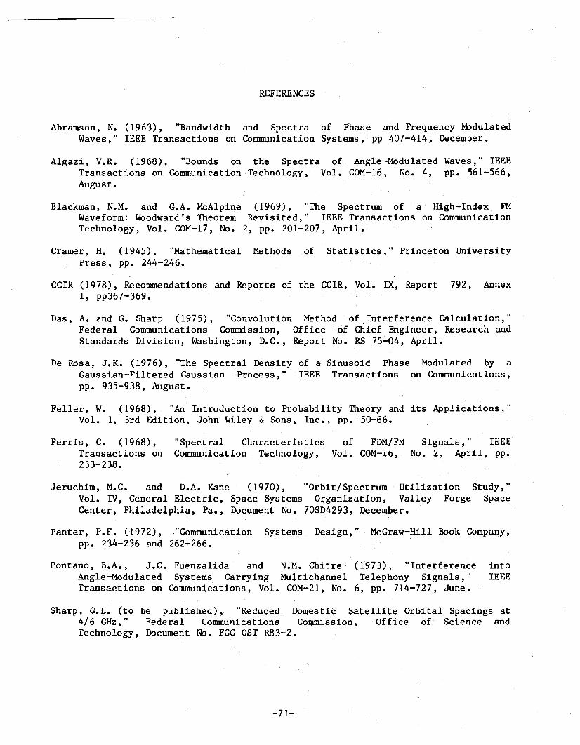
REFERENCES

Abramson, N. (1963), "Bandwidt1h and Spectra of Phase artd Frequency ModulatedWaves," IEEE Transactions on Communication Systems, PP 407-414, December.

Algazi, V.R. (1968), "Bo'unds on the Spectra of Angle-Modulated Waves," IEEETransactions on, Commu'nication· Technology, Vol. COM-16, No.4, pp. 561-566,August.

Blackman,N.M. and G.A.McAlpine (1969), "The Spectrum of a High-Index FMWaveform: Woodward's Theorem Revisited," IEEE Transactions on CommunicationTechnolo:gy, Vol. COM-I]', No.2, pp. 201-207, April.

Cramer, H. (1945), "Mathematieal Methods of Statistics," Princeton UniversityPress, pp. 244-246.

CCIR (1978), Recommendations and Reports of the CCIR, Vol. IX, Report 792, AnnexI, pp367-369.

Das, A. and G. Sharp (1975), ·'Convolution Method of Interference Calculation,"Federal Communications Commission, Office of Chief Engineer, Research andStandards Division, Washington, D.C., Report No. RS 75-04, April. .

De Rosa, J.K. (1976), "The Spectral Density of a Sinusoid Phase Modulated by aGaussian-Filtered Gaussian Process," IEEE Transactions on' Colnmunications,pp. 935-938, August.

Feller, W. (1968), "An Introdu.ction to Probability Theory and its Applications,"Vol. It 3rd Edition, John Wiley & Sons, Inc., pp. 50....66.

Ferris, C. (1968),Transactions on233-238.

"Spectral CharacteristicsCommunication Technology,

of FDM/FMVol. COM-16,

Signals," IEEENo.2, April,pp.

Jeruchim, M.C. and D~A.Kane (1970), "Orbit/Spectrum Utilization Study,"Vol. IV, General Electric, Space Systems Organization, Valley Forge SpaceCenter, Philadelphia, Pa.,Document No. 70SD4293, December.

Panter, P.F. (1972), "Comm.unicati,on Syst~ems Design," McGraw-Hill Book Company,pp. 234-236, and 262-266.

Pantano, B.A., J.C. Fuenzalida and N.M. Chitre (1973), "Interference intoAngle-Modulated Systems Carrying Multichannel Telephony Sign,als, It IEEETransactions on Communications, Vol. COM-21, No.6, pp. 714-727, June.

Sharp, G. L. (to be published) ,. "Reduced Domes tic Satellite .Orbital Spacings at4/6 GHz," Federal Communications Co~ssion, Office of, Science andTechnology, Document No • FCC OSTR83-2.

-71-

APPENDIX A

FM BAN,OOIDtHANDPOWER DISTORTION

The identification of a finite bandwidth measure for the FM signal spectraimplies a spectral tail truncation and a power preservation compromise. Theeffectiveness of a bandwidth measure to accommodate the FM signal spectrum isalso critical from an analytical simulation standpoint. The' number of pointsamples involved' in discrete' representations is necessarily finite" so that itinduces aliasing and distortion effects that limit the sp~ctral analysisaccuracy.

The approach usually employed for analog FM bandwidth assignment has beenCarson's Rule. TheFM bandwidth is given by B = +(~Fp+ f m) = 2(a+l)fm, where fJFis the peak frequency deviation, a, is the peak modulation index 'and fm is thepeak modulating frequency. This rule represents an additive combination of thebandwidth expressions for. extreme high (B~. 2~Fp= 2afm) and low (B ~ 2fm) indexconditions. One of these two' expressions prevails over the other for a» 1 ora« 1, so.that their linear superposition always yields the bandwidth measure forextreme index conditions.

The distortion implications of Carson's Rule as a' function of the modulationindex remains an open issue. There is no distortion measure or criterion that isgenerally accepted for evaluation purposes, with the difficulties arising fromthe variety of modulating signal characteristics and models that occur inpractice~ The discussion that follows concentrates on power preservation as adistortion measure for a deterministic (single sinewave) and random (uniformspectrum) baseband modulation cases.

One ·,distortion criterion is based on the magnitude of the sidebandspreserved or rejected when band-limiting the modulated signal spectrum. In thecase of single sinusoidal modulation, the number ~. (a ),?f sig.nificant sidebandpairs .~o.·.bepreservedcan be established as a function of the index (a) for agiven· significance level (v) from the condition ,IJM(a.)I2. u w~ere J(.) is theBessel function of the first kind. The FM bandwidth measure is then given byBu(a) = 2Mu(a)fm, and varies with the level (u) selected be,sides the index (a).This bandwidth allocation procedu·re has been compared to Carson's ,Rule to showt'hat the latter represents an FM bandwidth assignment with a significance levelin the 0.01 <u< 0.1 range for all practical modulation indices when themodulation is a single sinusbid.

Another distortion criterion corisists of the power percentagepreserved or rejected when band-limiting the modulated signal spectrum.singl,e .~sinusoidalmodula,tion,thepower percentage preserved is given by

PM(a) = J o2(a) + 2 r I n 2(a)

n=l

beingFora

(A-I) .

when n 1 to M sideband pairs are maintained. The number of pairs Mp(a) needed

-72-

for a given power :'percentage (p) can be found from this relation,and the FMbandwidth measure is then given by B (a) = 2M (a)f m• The normalized bandwidth2M p<a) can be evaluated independently of~the modufating frequency (fm).

The normalized bandwidth is shown in Figure A-I for va,rious powerpercentages to be preserved. Each step function corresponds to a fixed powerpercentage (p), with the solid step function representing p = 99% powerpreserved. The normalized bandwidth assignment based on Carson 's RU.Ie is givenby 2( a + 1), which is represented in the figure. by the solid straight line. Therule is noted to essentially follow the p = 99% curve steps for i.ndices in the0.9 < a < 4.3 range. It also preserves more power at lower indices, but fallsprogressively below the 99 percent power curve at higher indices outside thisrange.

The case of a random modlllating signal With a uniform baseband spectrum hasalso been analyzed using preserved power as the band ....limiting distortioncriterion. A peak to rms load ratio of 11 dB has been assumed to simulaterepresentative conditions of FDM/FM telephony, and the resultant bandwidthmeasure B q(a) = 2Mq(a)f m is obtained from the folloWing relation

(A-2)

where q = 1 - (p/lOO) represents the powerf'ractionrejected. This iexpression isan effective approximation to a complicated integral fo~mulation :for moderateindex values (1 < a < 5). The normalized .bandwidth 2Mq (a) is shown 1n Figure A-2for various (q) values, alon.g with the bandwidth assignment corresponding toCarson's Rule. 8 The latter can be noted to represent a power rejection in the10 -10< q < 10 - range, which is negligible.

The two modulation cases analyzed here correspond to extreme distributionconditions, in that one has all .the· baseband energy concentrated ona slnglefrequency while the other llas it spread uniformly over a frequency band. Theimplication of Figures A-I and A-2 is that Carson's Rule represents a rathereffective approach to the analog 'FM bandwidth assignment from a powerpreservation standpoint when modulation indices below five radians areconsidered. The results also indicate that Carson's Rule preserves considerablymore power when the baseband modulation has a spread rather than concentratedspectral characteristic.

References

(A.l) Carlson, A.B. (196~), "Communication Systems," McGraw-Hill Book Company,pp. 239-243.

(A.2) Plotkin, S.C. (1967),Modulation ,Index," IEEE46i-470 (June).

"FM BandwidthTransactions on

-73-

as a FunctionCommunications

of Distortion andTechnology, pp.

p=99.99%r._._ ..,..... 0

i.Ir._.....; ........_....L p=99.9%. . .' .

I ·i• . : p=g9%r. - ......~...... ··.1. • .... • • • • • • • • ]II. : I

! : II ·• p~9-0%;-r· ·--·_·· r----

. : I

I : I· · II : I

.-~-.~ 1.. :..... •• · r--- ~-~--_.J-I· : I. • I1 : I· I".-._.__ t- ..J

! : II · I. II ~~~_~_--_~

21·~ I .. J J

12

14

16

,,-.. 104-4

8...........P=l"-'

is 8~H

2SI ~

'-JJ:'

~

I 6~I::t.lNH

~ 40z

oMODULATION INDEX

Figure A-i. FMBandwidth Occupanc:y and Power Preservation with Sinusoidal Modulation.

(:Note: 'Carson's Rule is the Straight Line)

(Legend: P is the Power Percentage P~~serve~)

14

12

;e10~'-'

~E-tAH

g 8<~

~~l

NH....:l

~ ~ 6oz

4

1.5 2.0 2.5 3.0MODULATION INDEX (a)

3.5 4.0

. Q=10-2

4.5 5.0

Figure A-2. FM Bandwidth Occupancy and Power Preservation with Band-Limited ltlhiteModulation.

(Note: Carson's Rule is the Dotted Line)

(Legend: q is the Power Fraction Rejected)

(A.3) Medhurst ,R.G. and Plotkin, S.C. (1968),Functio,n of Distortion and ModulationCommuni'cat~on,Technolog.y" ."p. 500 (June).,

-76-

"Colnments' on FM Bandwidth as aIndex," IEEE Transactions on

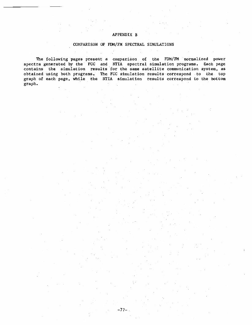
APPENDIX B

COMPARISON, OF FDM/FM SPECTRAL SIMULATIONS

The following pages pres~~t a comparison of the FDM/:FM normalized powerspectra generated by the FCC and NTIA spectral slmulatio.n progra.ms. Each pagecontains the simulation reslJlts for th'e same satellite communication ,system) asobtained using both programs. The FCC simulation reS,tilts correspond to the topgraph of each page, while the NTIA simulation results cor'respond to the bottomgraph.

~77-

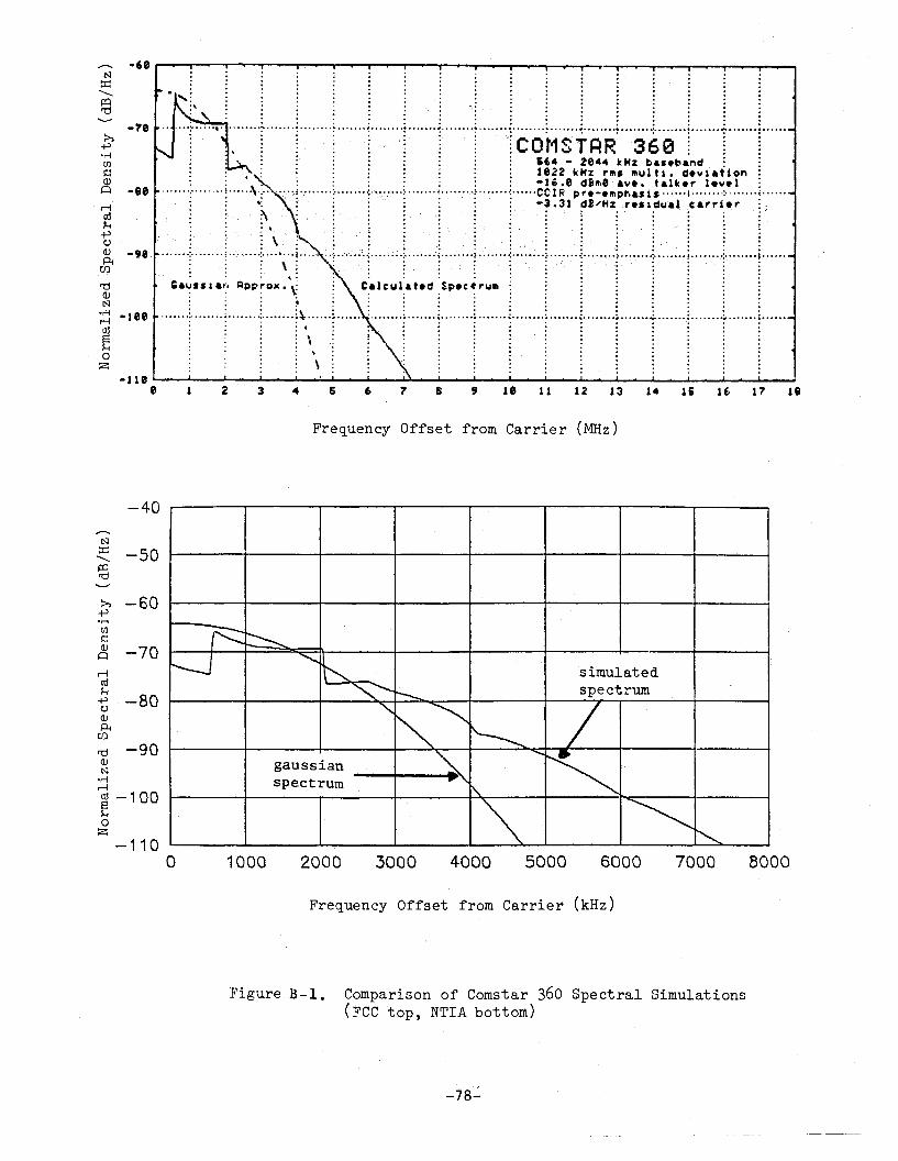
• 0 0. .. .....······.·1·· .. ···~········[···· ..·Tc·6't1·S+·A~(··i6·e ..T·······f···· ..· ......

. .: ..:: '£4 -2e44 k HZ. t>~••band .: . .: :: ::: :1822 kHz ,."'. Irtul ti. d.viation

......L i :·,tN·~··~, ~.L ,L -=,' ; !.. ; ..:, .. .L ·c;MR"ep~:~:ftI" :~:; i :~.~~.~i~•••l.~.~~ .1•••••••••••~ ~ .: ,',. ;. ~ ~ . ~ ~ ~ ~ - ~ .31~ J "~z~,r•• l.dua~.Ca,. r i.• ,.: :'.\ "'C,,: ;", : :.:.: :: : : : : :

. ~ . ~ ~ \:' 1 j ~ ~ ~ ~ j ~ '~ ~ j ~. '. ~"'.. ',: .' . ~ . ::. - ., ,'.: '. ',. . ., -'. - , '. ...... ." . ...•.•••:~ .•••.•• : ~ ...•"...... -:•.•.•. ~" .•,i···· .,.. ,e••.::- - ...."'•.•• '~ .: •••• '.; •• :-:". ~~'". ~ ;,- ~. ~ ~ .'•• : ••••••• •:· ••••••• i .•..••• .:•••..•,.•:.• e,: •••••:•••••••• ! ...•' ...•.•:•.....•

: : ; \: ; :: .. ': . : ~ : ! :

'a~"U~1 AP~~O)(. \ C"lCloIl;at.d :SP.C~,.Utll ~ . :.:

...... I····· .. !······· .~ f\···J : ! 1········!··.. ··· i·· ~ ····~··· ..·..t·· ..···I··· ~ I· ·· ..:: :: ': : :

~ ~ \ ~ : ~ ; ;11 11 12 13 14 15 1£ 17 18,876s32

-11 e .....................---_....a.-..............-...;~.................--......................._. ......._._.""'__'"""_....... __r_......................__......--..---.........----~.......

e

Frequency Offset from Carrier (MHz)

-40

N~ -50..........,:Qrd

>:, -60-+JoMens::Q) -70A

--~~N '"~ simulated

~spectrum

~

~~ /~~ "'"'

~gaussianspectrum r,

"~ ~

~

1000 2000 3000 4000 5000 6000 7000 8000

Frequency Offset from Carrier (kHz)

Figure B-1. Comparison of Comstar 360 Spectral Simulations(FCC top, NTIA bottom)

-78-

181116:1614131211II

· . . . .· ,.. ." '" . . ." .•. , •. , •••• ~ •• _. - ~ •••. ' •••••• _._ •••••••••• ~ •••• t ••••••••••••••••· . . . ., .· . . .. .., .. .· ..· .· .· .· .· .· .

,

· . .. ., ......:.. '"~.." : : ~ : .....•:.,': '...•. : : : : '.•' ! ...•..· . . . . . . . . ..· . . .. .. .· . .,.· .· .· .,.· .,.· .

... . .. .. ·······i········:·······:········:·······1"·······:···· ···r·C'()M·S·T·RR····6·~i0··1·······r·· ..···j······

: : ~~: ....: 16'4 - 3884 kHz bas.band; :: :. . :'.: : : : :. 1811 kHz, rms' MU 1 t.i '. d.,,· i a,t 1on :: . :': .~.~....:, : : :. :-16.edB"'e,."•• talk.r It,,.l;.....··r oo

1' f····· \,~'" C'" 'T'00.'.1"' T' 00 1' "Si~;5"d;~~;P~::: :~~i!' ~.~.; '~:i'~';" T' ... ... .. .· ,. . .'· .

......~ i ) i ~ ~ ~..· . . . . . , .: ~ ~ : ~,,\ ~

'::;aussian ~ppro~i,.ation ~

: : : , : ' : :..... . ~ 'f······ ':' ": ','x,' ..: e •• '~."

, :

-8e

-ree

Frequency Offset 'from Carrier (MHz)

-40

,2000 6000 1000'C) 12000

Frequency Offset from Carrier (kHz)

Figure B-2.. Conlparison of Comstar600 Spectral Simulations(FCC ~op, NTIA bottom)

-79-

1£

r-fro~

+>~ -,e~

tf)

rd(1)N

e,-; -seer-Iro~o~

-11 e '--~.&.i-"""'- ~~....,.. ~~~~ ~~ ""'-''''''''''''~~'''''''''''''''''''''''''''''''''''''''-''e·'·~:~lal·3

-6'",-....

N~""-..

~-11

:>:>+>e,-;en~(1) -Ie~

Frequf;l1 CY Offs~t fro!Il Garrier(MHz)

--70

--90

80QO 10000 1200Q 14000 16000 1~OCO60002000

.-eo

-110o

r-fro~

+>()(1)

PICJ:)

rd(1)N

e,-;r-fro~ ~100o~

-60

-50

Fr~q~~ncy Offset from Carrier (kHz)

figure B-3. Comparison of Comstar 1200 Spectr~l Simt1,lations(FCC top ,NTIA bott9ril)

-80-

FreqllencyOffset from Carrier (MHz)

25000.2000015000

simulated~spec·trum

100005000

gaussianspectrum ~--~~~~

-50

t:'I~ -60............~ro

~ -70+J.,-iens::(1)A

....-f -80cd~

+Jt>(1) -90~

(f)

ro(J)t:'I

.,-i -100....-fcdS~0z ..... 1.10

'0

FrequencyO~fset from C~rrier (kHz)

Figure :3-4. Comparison of Telstar 1800 Spectral Simulations(~CCtop, ~TIAbottom)

-81-

.: .

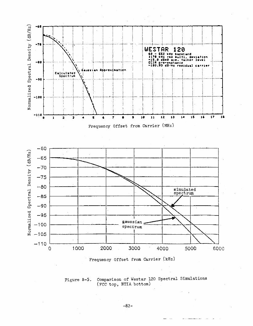
IWESTRR 120· 60 -5S2 kHz ba•• t 6nd

Il1ekHz r•••~J~j. ~.vj.~j~n-l£~e dl.e av•• talk., l.y.lCCIR ~'.-.~~~ar1'-180.93 d)'H~ , •• ~~wal car,t.r

1. 11 12 13 14 15 16 11 11

. . . . .: •.•••• ~ •••••• '. '~" ••••• ' ~ •••• tl ••• : .••••••••: •••••••• ~ •••••••

,•,432

. .•. ',: .':" .• . e:, _'., •',." ···T.;········· .. ,···;·······,1········f···· ... ~.....

• • 0· ..

~: ••• • • f • i' :- •.••• " •.: ~ . . . . .. .:.... . •..:· .· .· .· .. .-..: : ;., ;a...... i·an ApI'rcxi ••tion : :: C.l c,-,Iii t .d I: ::":: :: Sc:·~c t r~",:\; : : : : . : . . : : . .

·······r·······~·········:······· ·········j·······r·····r·····~········~·······~········r ·· ..··r....T......·:....···r..·..r....·T....·. .. . .. .. . ... .o' •.' 0

.' 0.., ..••••• • : ••••••• ; ••••••• 0:.0 •• 00 •• ; •••••• ~ •••• o' ~~••• o .f •• : ••••••••••••••••~... • .~••••••••~.••••.••• ~ •• 0 ••• o.~ ••••••••~ ••••••• : 0 •••••••: •••••••• : ••••••.. . ... ... .· . .. .

• t" •· . . .· . . .· . . .· . . .· . . .· . . .· . . .-11 e '--- .--.....-.....-. -- .-.. ......- _ .......

e

~ -6' .--....- ....-..,.-...-...,... ...,.. -.... -... --. ~ ,.-..- ....- -.- ~~

::q.............

~

Frequency Offset from Carrier (MHz)

~-60

N::q

-65.............

~

>: -70+'.r-f

-75ens::(J)

~ -80.--iro~ -85+'()(1)

~ -90enI'd(J) -95N

er-f..-1

@ -1000

-105z

-l100 1000 2000 3000 4000 5000

Frequency Offset from Carrier (kHz)

Figure B-5 .. Comparison of Westar120 Spectral Simulations(FCC top,NTIA bottom)

~82-

18

...••. : .; ! :......•.......

11 1, 13 14 16 16 11

WESTRR "18068 - 8e~ kHz ba••ba~d12SB kHz r •• -ulti. d.viatlon-1£.8 dJ~e av•• talk.r l.v.1CCI~ ~r.-.~~~a.j.-11.4& dl/Hz r.slGual carrl.r

. "

....... ~ ~ ~ ~ ~ ';' : .• • • • II •· . . . ., .· . . . " ... ..,... ".•• o.•• 0

•• 1I.. "•• II

•• t).. "

9 Je

....... ;. .

81,32J

,,: ....;\':.~.~~~.~.;~~;.~~~~.~~~.~.~~~.~~ .

· :, : : : : :· . .. . . . .: : \ : : : :

......+ ! :\l.~~ ~ ~ ~ .· . . . . . .• • • 1\. • • •

~ ; ~ .~ ~ : ; ~

~ ~ ~ . ~ ~ ~.......~ ~ ~ ···i· , ~ : ~ .

: :: : ::: ~ : .

-11>:+'·n(f)

s::(lJ

~ -Ie.-;m1-;

+'CJ(lJ ·,ep

U)

rod(lJN

~ -leecO

~o~

-III '--~.a.-........-__..........--.__......-L..- .-.-........ .-.........-.-..--.........__......-_.......~............-.....&-........-........--.t_................;

•

,,-... -6e r--.-.,.........-..,.............,.........--r-......,-....-,...........,--......-r-........,..~--r'-.....,-,..--r--....--r--.........,.--.--r--......................-,.......N

::c:'-.....

~

F'requency Offset from Carrier (MHz)

700060005000

---~----,----- ._-_...0.--4

300()

gaus s ian __~-----...."-J

spectrum

2000

..----.---- --------- .---._---t------I-.------. -_._--

9------- -----..-------.,..-----__----_ ------,

1000

t-----------_+_

~-----------f------+------+-~:___~-_+--..;;...I;;...;::...;;~1~·----

t------ ---',---;------·J-----4

-60N

::c: -65'-.....

~-70

:>,+'·n -75(f)

s::(lJ

~ -80.-;m

-851-;+'CJ(lJ

-90P..Cf)

"d -95(lJN

·n.-; -100cOs1-;0 -105~

-1100

Frequency Offset from Carrier (kHz)

Figure B-6. COTIlparison of Westar 180 Spectral Simulations(FCC top, NTIA bottom)

-83-

FORM NTIA-29(4-80)

U.S. DEPARTMENT OF COMMERCENAT'L. TELECOMMUNICATIONS AND INFORMATION ADMINISTRATION

BIBLIOGRAPHIC DATA SHEET

1. PUBLICATION NO. 2. Gov't Accession No. 3. Recipient's Accession No.

NTIA REPORI' 83-134

4. TITLE AND SUBTITLE 5. Publication Date

FM SPECTRUM MODELING AND FDM/FMSIMULATION PROGRAMS

September, 19836. Performing Organization Code

7. AUTHOR(S)

Cesar A. Filippi8. PERFORMING ORGANIZATION NAME AND ADDRESS

National Telecommunications andInformation Administration

179 Admiral Cochrane DriveAnnapolis, Maryland 21401

9. Project/Task/Work Unit No.

9014101

10. Contract/Grant No.

11. Sponsoring Organization Name and Address

U.S. Dept. of Commerce/NTIA179 Admiral Cochrane DriveAnnapolis, Maryland 21401

12. Type of Report and Period Covered

Technical

13.

14.--StjPPl::EMENTARY NOTES

16. Key Words (Alphabetical order, separated by semicolons)

15. ABSTRACT (A 200-word or less factual summary of most significant information. If document includes a significant bibliography or literaturesurveYnl!1ention it here.l •

Ln1S repOrL 1S concerned with the spectral representation of analog FMsignals, with particular attention to FDM/FM satellite communication systems.The FM spectral modeling and ga.ussian approximation principles are analyzed andextended to develop computer simulation programs capable of providingrepresentative FM spectra. A generalized program is developed to accommodate avariety of baseband and preemphasis characteristics, and adapted to generateFDM/FM telephony spectra. Th,e program features the automatic validation andgeneration of the gaussian spectrum model if applicable, or the automaticsimulation of the modulation process to generate the FM spectrum samplesotherwise. The program is used to simulate a collection of satellite FDM/FMtelephony spectra, which are to be applied as input data into other availableinterference analysis programs, as part of a major automated computer capabilitydedicated to the comprehensive assessment of orbital congestion and spectrumresource management concerns pertinent to national and international satellitecOrnmtlojcation systems scenarios.

FM Spectrum Models; Gaussian Spectral Approximation; FM Spectrum Simulation;

FDM/FM Telephony Spectra

17, AVAILABILITY STATEMENT 18. Security Class. (This report) 20. Number of pages

lli! UNLIMITED. UNCLASSIFIED 92

o FOR OFFICIAL DISTRIBUTION.

19. Security Class. (This page)

UNCLASSIFIED

2'1, Price: