Fm Sem - Inventory RSP

8/12/2019 Fm Sem - Inventory RSP

http://slidepdf.com/reader/full/fm-sem-inventory-rsp 1/17

5 - 1

Copyright © 2009 by R. S. Pradhan. All rights reserved.

Welcome to the sessionon

Estimates of Inventory Demandby Nepalese Corporations

Research in Nepalese Finance



5 - 2


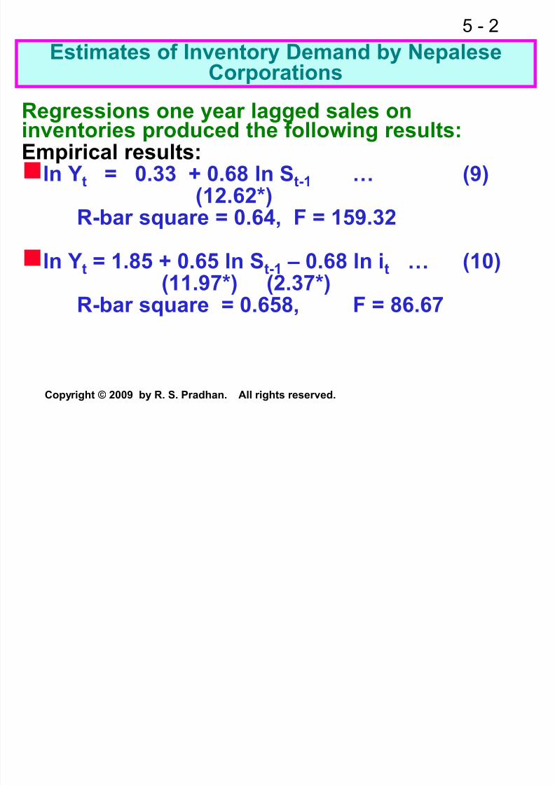
Estimates of Inventory Demand by NepaleseCorporations

Regressions one year lagged sales oninventories produced the following results:Empirical results: ln Yt = 0.33 + 0.68 ln St-1 … (9)

(12.62*)R-bar square = 0.64, F = 159.32

ln Yt = 1.85 + 0.65 ln St-1 – 0.68 ln it … (10)

(11.97*) (2.37*)R-bar square = 0.658, F = 86.67



5 - 3


Regressions of current year sales on inventoriesproduced the following results:

ln Yt = 0.33 + 0.69 ln St … (11)(12.57*)

R-bar square = 0.638, F = 157.98

ln Yt = 1.99 + 0.65 ln S

t – 0.76 ln i

t … (12)

(12.07*) (2.67*)

R-bar square = 0.662, F = 88.07

The partial adjustment model results:

ln Yt= –0.78+0.08 ln St-1 –0.43 ln it+0.85 ln Yt-1 (13)

(2.62*) (2.27*) (15.23*)

R-bar square = 0.889, F = 238.55

xxx



5 - 4


Estimates of Inventory Demand by Nepalese

Corporations

Statement of the problem

There is no controversy as to the fact that

target inventory level is a function of expectedsales as indicated by almost all the earlierstudies on the demand for inventories by firms.

The controversy arises as to the presence of

economies of scale in inventory holdings, thecost of capital and other effects on inventorydemand, and the adjustment speed of actualinventory level with target inventory level.



5 - 5


Among others, Irvine (1981 May, 1981September) and Akhtar (1983) clearly indicated

economies of scale in inventory holding.

However, some of the inventory demandfunctions of Lieberman (1980) showeddiseconomies of scale.

Much of the controversies, however, exist withthe cost of capital effect on inventory demand.

Theoretically, the level of inventories of a firm

would depend on the costs associated withholding inventories.

However, the earlier studies on the demand forinventories did not present unanimous findings.



5 - 6


Liu (1963, 1969), Kuznets (1964), Lieberman, Irvin and Akhtar reported statistically significant

effect of capital costs on the demand forinventories.

However, Robinson (1959), Lovell (1961, 1964),Burrows (1971), Joyce (1973), and Maccini and

Rossana (1981) did not report the same.Controversy also exists with respect tocoefficients of adjustment.

Among others, Burrows, Maccini and Rossanaand Irvine observed faster adjustment betweenactual inventories and target inventories.

While Lovell and Grossman (1973) observedslow speed of adjustment.



5 - 7


Thus, there is no unanimous finding withrespect to:

- economies of scale in inventory holdings,

- capital costs effect on inventory demand, &

- adjustment coefficient of actual inventories to

desired inventories.

It has therefore become difficult to support one view or another as there exists no suchstudies in the context of Nepal.



5 - 8


I. The ModelThe decision about the aggregate level ofinventories to be held may be regarded as

subject to the constraint of wealth and the cost ofholding inventories.

As a first approximation to the theory, thefunction may be written as,

Y* = f (S, i) ... (1)Where, “Y*” is real desired level of inventories,“S” is the real desired wealth defined in terms ofsales, and “i” is the holding cost.

In an empirical investigation, expression (1)takes the form.

Y* = k S b1 i b2 eu … (2)

Where, the error terms eu is assumed to beindependently and normally distributed.



5 - 9


Taking the natural logarithm of the expression(2) gives,

ln Y* = ln k + b1 ln S + b2 ln i + Ui … (3)

It is assumed that the desired level ofinventories (Y*) is equal to its actual level (Y).Thus, the equation to be estimated is,

ln Y = b0 + b1 ln S + b2 ln i + Ui … (4)

Where, b0 is constant, b1 and b2 are elasticitiesof Y with respect to sales and holding costs

respectively.The above model assumes the followingreasonable a priori hypothesis:

δy/δs > 0, & δy/δi < 0 … (5)



5 - 10


While estimating the above equations,inventories and sales have been deflated by usinga deflator.

The empirical analysis also takes into account apartial adjustment or flexible accelerator model ofinventory behaviour.

This model hypothesizes that each corporationhas a desired target level of inventories, and that

each corporation, finding its actual level ofinventories not equal to its desired level, attemptsonly a partial adjustment towards the desired

level within any one period.The partial adjustment model is used toindicate the speed with which corporations adjusttheir actual level to desired level of inventories.



5 - 11


The partial adjustment model is stated as,

ln Yt=c0+c1 ln St+c2 ln it+(1 – θ) ln Yt-1+Ut … (7)

Where, θ=rate of adjustment coefficient, c1 & c2 are the short run elasticities of inventories withrespect to sales & interest costs respectively.

Long run elasticities with respect to sales &

interest costs are b1 and b2.Since c1 = θb1 and c2 = θb2,

b1 = c1 /θ & b2 = c2 /θ … (8)

Short-term interest rate of commercial bankshas been used as a proxy for holding cost of

funds invested in inventories.



5 - 12


Empirical ResultsThe regression of inventories on salesproduced the following result:

ln Yt = 0.33 + 0.68 ln St-1 … (9)(12.62*)

R-bar square = 0.64, F = 159.32

The elasticity of sales with respect toinventories is less than unity showing evidence ofeconomies of scaleIt thus supports the findings of Akhtar and

Irvine and contradicts unitary or more thanunitary sales elasticities noticed in some of theequations of Lieberman.Equation (9) ignores the opportunity cost offunds invested in inventories.



5 - 13


The regression of inventories on sales andcapital cost produced the following:

ln Yt = 1.85 + 0.65 ln St-1 – 0.68 ln it … (10)(11.97*) (2.37*)

R-bar square = 0.658, F = 86.67

Interest rate coefficient is statistically

significant with a theoretically correct sign.Previously, this coefficient used to be eitherpositive or not significant in many of the studieson the demand for inventories by firms.

The highly significant coefficient of sales isconsistently less than unity in equation (10).

It shows evidence suggesting economies ofscale in inventory holding.



5 - 14


This finding supports the conclusions of Liu,Kuznets, Lieberman, Irvine and Akhtar.

And contradicts with the results of Robinson,Lovell, Jon Joyce, Burrows, and Maccini and

Rossana.

Holding the sales constant, it indicates that a

one percentage point increase in capital costleads on an average to about a 0.68 percentdecline in inventory investment.

Similarly, holding the capital cost constant, a

one percentage point increase in sales leads onan average to about 0.65 percent increase ininventory investment.



5 - 15


So far the estimated results are based onprevious year sales (St-1).

These results may not be directly comparableto results of some of the earlier studies whichused current year sales (St) as an explanatoryvariable so long as the results are similar.Hence, it is felt necessary to use St instead of

St-1.The regressions of Yt on St, and on St and it produced the following results:ln Yt = 0.33 + 0.69 ln St … (11)

(12.57*)R-bar square = 0.638, F = 157.98ln Yt = 1.99 + 0.65 ln St – 0.76 ln it … (12)

(12.07*) (2.67*)R-bar square = 0.662, F = 88.07



5 - 16


The use of St-1 or St produced similar results.

After assessing the scale effect and cost of

capital effect on inventory demand, we nowestimate the partial adjustment model ofinventory demand.

The pooled estimate of the partial adjustmentmodel is as follows:

ln Yt = –0.78 + 0.08 ln St-1 – 0.43 ln it + 0.85 ln Yt-1 …(13)

(2.62*) (2.27*) (15.23*)

R-bar square = 0.889, F = 238.55

In equation (13), the coefficient of the laggeddependent variable has been observed to be 0.85.

Since the coefficient of lag ln Yt is equal to 1minus the adjustment coefficient (1-φ), theadjustment coefficient is equal to 0.15.



5 - 17


The speed of adjustment between desired andactual inventories as implied by this value ismuch slower, about 15 percent.

The result therefore contradicts the high speedof adjustment observed by Burrows, Maccini andRossana, and Irvine.In the partial adjustment model, the estimated

coefficients of the independent variables areequal to the elasticities of these variable times theadjustment coefficient, e.g., c1= θb1 & c2= θb2,b1=c1 /θ & b2=c2 /θ. These coefficients are thus.08/.15=0.53 for sales & .43/.15=2.87 for interest

rate which again support the conclusions drawnearlier.The capacity utilization as a significant variableaffecting the demand for inventories is doubtful.

THANKING YOU

Documents

Fm Sem - Inventory RSP