FLUOROSNNAP! - Penn Engineeringmolneuro/FluoroSNNAP/user_guide.pdfFLUOROSNNAP! UserGuide! ©2015! FluorescenceSingleNeuronandNetworkAnalysis! Package! Tapan!Patel,!PhD! University!of!Pennsylvania!

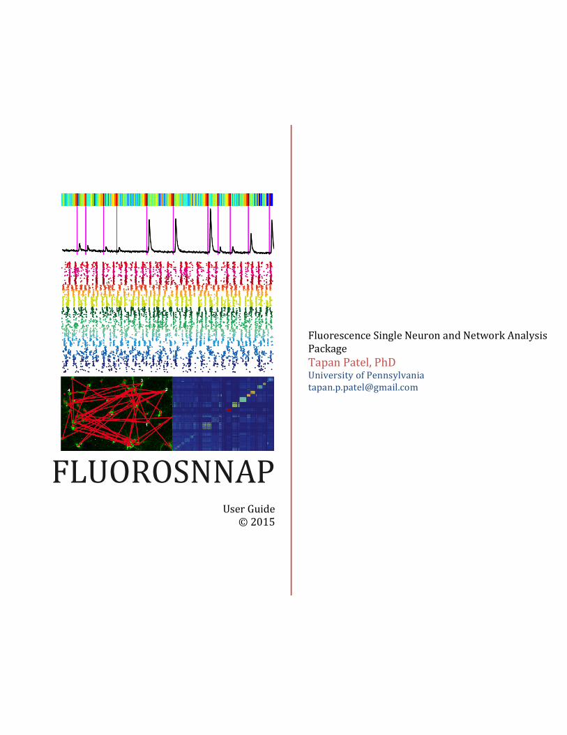
FLUOROSNNAP User Guide

© 2015

Fluorescence Single Neuron and Network Analysis Package Tapan Patel, PhD University of Pennsylvania [email protected]

FluoroSNNAP user guide

1

Table of Contents

GETTING STARTED 3

General comments 3

Installation 3

Sample Pipeline 4

Detailed descriptions of each menubar item 4 File menubar: 5 Batch segmentation pushbutton: 6 Pre-‐processing menubar 8 View image stack 8 Remove bad frames: 8 Motion correction 8 Check for motion artifact: 8 View correlation matrix 9 Overlay pair-‐wise frames: 9 Align pair-‐wise frames 10 Align all frames to a template 11 View corrected stack 11 Save image stack 11 Preferences 11

Segmentation GUI. 11 File menubar (in the Segmentation GUI) 12 Edit menubar (in the Segmentation GUI) 12 Tools menubar (in Segmentation GUI) 13

View Segmentation 15 Batch segmentation 15 Time-‐averaged image 15 Maximum projection 15

Analysis menubar 16 Preferences 16 Choose analysis modules 16 Parallel computing 16 Acquisition frame rate 16 Baseline fluorescence (F0) 16 Calcium event detection 17 Synchronization Analysis 17 Functional connectivity 17 Spike Inference 18 Network Ensemble 18 Revert to default 18

Process single file 18 Batch single and network-‐analysis 18 Template library 19 View calcium waveforms: 19 Add a calcium waveform to library: 19 Delete a waveform from library 19

Recompute synchronization and functional connectivity 19 View menubar: 21


2

Fluorescence traces: 21 deltaF/F0 traces 21 Raster plot (calcium): 21 Raster plot (calcium, grouped by activity) 21 Calcium event inspector: 22 Tools 23 Remove calcium event: 23 Add calcium event: 23 Set a new threshold and apply to selected ROI 23 Set a new threshold and apply to all ROIs 23

Synchronization matrix: 23 Summary figure: 25 Functional Connectivity 25 Cross-‐correlation 25 Partial correlation 26 Instantaneous phase 26 Granger causality 27 Transfer entropy 27

Fast spike inference 28 View spikes 28 Inferred activity raster 28

Network ensembles 28 Controllability 30 Single cell summary 31

ADVANCED USE 31

Segmentation 31

CaSignal 32

Analysis 32 Synchronization 34 Functional connectivity 35 Single-‐cell descriptors 38 Network ensembles 40

HOW TO CITE: 40

REFERENCES: 41


3

Getting Started

General comments We created a set of MATLAB routines and graphical user interfaces to facilitate the analysis of calcium fluorescence imaging experiments of neuronal activity. The Fluorescence Single Neuron and Network Analysis Package (FluoroSNNAP) directly accepts .tif stacks of image activity or pre-‐processed .csv files containing fluorescence vs. time data. The main steps of the analysis are segmentation, event detection, and network inference. Segmentation is the process of identifying individual neurons in the field of view. Event detection includes methods to detect when each neuron displays a calcium transient that is distinct from noise fluctuations in fluorescence. The network inference is an assortment of techniques to estimate several network connectivity metrics from a video segment. All of these tasks are automated and the user can interactively work on different steps of the pipeline with the GUI. The only software requirement is MATLAB 2013b or MATLAB 2014a (no additional toolboxes other than the basic toolboxes are required). Note: GUI layout maybe different and unusable in MATLAB 2014b. Image processing is inherently memory intensive and we recommend having at least 8GB RAM (ideally >16GB). To date, we have tested this software on Mac OS/X (10.9), Windows 7 (64bit) and Linux (Ubuntu 14.04) machines. If MATLAB is running correctly on these machines (full install, including the available analysis packs), the software should run through the example data without any problems. If there is motion artifact in your experiments, use ImageJ plugins prior to using this software to help correct for motion artifacts. We provide a set of rigid image registration routines that prove to be useful for small motion artifacts and sudden stage shift. We have not tested these algorithms on in vivo dataset with cardiac/pulmonary motion artifacts however. We provide sample experiments as a .tif stack and a .csv file for you to try the software (available on www.seas.upenn.edu/~molneuro/fluorosnnap.html). Download the baseline.tif file or baseline.csv file and place them in separate folders. We recommend placing all .tif files in one folder and all .csv files in another folder. For questions or comments for improvement, please email [email protected] and refer to the accompanying manuscript.

Installation -‐ Download the calcium image analysis software source code FluoroSNNAP from

http://www.seas.upenn.edu/~molneuro/fluorosnnap.html -‐ Unzip the FluoroSNNAP.zip package and navigate to FluoroSNNAP folder in

MATLAB. -‐ The software package has been tested on MATLAB 2013b and MATLAB 2014a.


4

Sample Pipeline Follow these overall steps to process your .tif image stack of calcium activity. Details for each tool option are provided in later sections.

1. Run “FluoroSNNAP” at the MATLAB command prompt from FluoroSNNAP directory. 2. Add folders containing .tif stacks or .csv files. 3. Batch segmentation (Pre-‐processing menubar). 4. Set Preferences for analysis. 5. Launch Segmentation GUI and load the segmented image. Modify it as needed and

save to return to the CalciumAnalysis GUI. 6. Process either the single file or batch process all files (Analysis menubar). 7. View results – raster plot, calcium events, network structure etc. (View menubar).

Detailed descriptions of each menubar item -‐ Run MATLAB and change the working directory to FluoroSNNAP -‐ Enter the command FluoroSNNAP at the MATLAB command prompt. -‐ We recommend placing all the image files for a given experiment in one folder. This

software can process multiple folders in batch mode. -‐ You will be prompted whether to use parallel processing routines. Select “Enable” if

parallel processing toolbox is properly installed on your computer, otherwise select “Disable”.

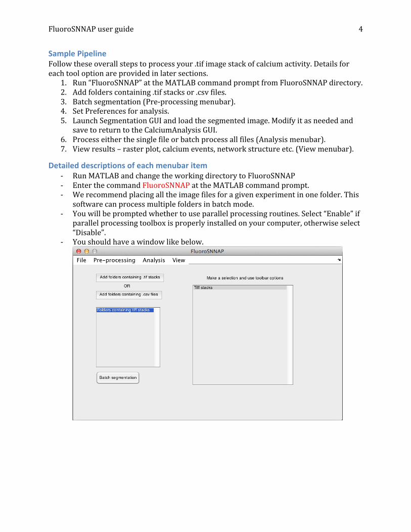
-‐ You should have a window like below.


5

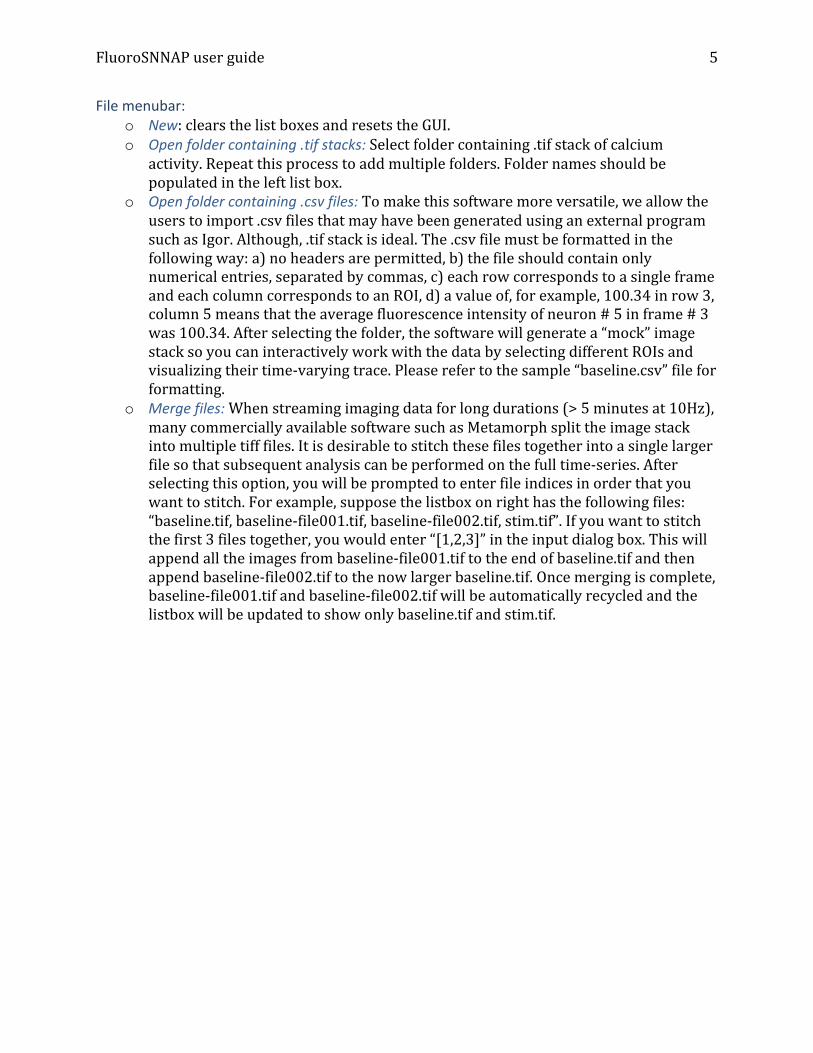
File menubar: o New: clears the list boxes and resets the GUI. o Open folder containing .tif stacks: Select folder containing .tif stack of calcium

activity. Repeat this process to add multiple folders. Folder names should be populated in the left list box.

o Open folder containing .csv files: To make this software more versatile, we allow the users to import .csv files that may have been generated using an external program such as Igor. Although, .tif stack is ideal. The .csv file must be formatted in the following way: a) no headers are permitted, b) the file should contain only numerical entries, separated by commas, c) each row corresponds to a single frame and each column corresponds to an ROI, d) a value of, for example, 100.34 in row 3, column 5 means that the average fluorescence intensity of neuron # 5 in frame # 3 was 100.34. After selecting the folder, the software will generate a “mock” image stack so you can interactively work with the data by selecting different ROIs and visualizing their time-‐varying trace. Please refer to the sample “baseline.csv” file for formatting.

o Merge files: When streaming imaging data for long durations (> 5 minutes at 10Hz), many commercially available software such as Metamorph split the image stack into multiple tiff files. It is desirable to stitch these files together into a single larger file so that subsequent analysis can be performed on the full time-‐series. After selecting this option, you will be prompted to enter file indices in order that you want to stitch. For example, suppose the listbox on right has the following files: “baseline.tif, baseline-‐file001.tif, baseline-‐file002.tif, stim.tif”. If you want to stitch the first 3 files together, you would enter “[1,2,3]” in the input dialog box. This will append all the images from baseline-‐file001.tif to the end of baseline.tif and then append baseline-‐file002.tif to the now larger baseline.tif. Once merging is complete, baseline-‐file001.tif and baseline-‐file002.tif will be automatically recycled and the listbox will be updated to show only baseline.tif and stim.tif.


6

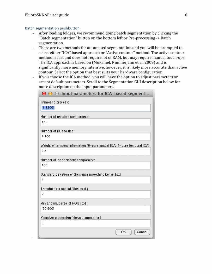
Batch segmentation pushbutton: -‐ After loading folders, we recommend doing batch segmentation by clicking the

“Batch segmentation” button on the bottom left or Pre-‐processing -‐> Batch segmentation.

-‐ There are two methods for automated segmentation and you will be prompted to select either “ICA” based approach or “Active contour” method. The active contour method is fast and does not require lot of RAM, but may require manual touch-‐ups. The ICA approach is based on (Mukamel, Nimmerjahn et al. 2009) and is significantly more memory intensive, however, it is likely more accurate than active contour. Select the option that best suits your hardware configuration.

-‐ If you choose the ICA method, you will have the option to adjust parameters or accept default parameters. Scroll to the Segmentation GUI description below for more description on the input parameters.

-‐


7

-‐ Once batch segmentation is complete, proceed by making a folder selection on the left listbox. The right listbox will be populated with .tif files from the selected folder. Make a file selection in the right listbox.


8

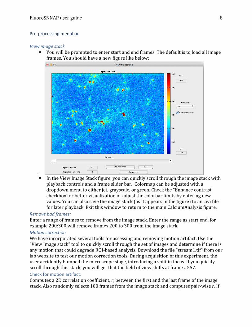
Pre-‐processing menubar View image stack

§ You will be prompted to enter start and end frames. The default is to load all image frames. You should have a new figure like below:

-‐ § In the View Image Stack figure, you can quickly scroll through the image stack with

playback controls and a frame slider bar. Colormap can be adjusted with a dropdown menu to either jet, grayscale, or green. Check the “Enhance contrast” checkbox for better visualization or adjust the colorbar limits by entering new values. You can also save the image stack (as it appears in the figure) to an .avi file for later playback. Exit this window to return to the main CalciumAnalysis figure.

Remove bad frames: Enter a range of frames to remove from the image stack. Enter the range as start:end, for example 200:300 will remove frames 200 to 300 from the image stack. Motion correction We have incorporated several tools for assessing and removing motion artifact. Use the “View Image stack” tool to quickly scroll through the set of images and determine if there is any motion that could degrade ROI-‐based analysis. Download the file “stream1.tif” from our lab website to test our motion correction tools. During acquisition of this experiment, the user accidently bumped the microscope stage, introducing a shift in focus. If you quickly scroll through this stack, you will get that the field of view shifts at frame #557. Check for motion artifact: Computes a 2D correlation coefficient, r, between the first and the last frame of the image stack. Also randomly selects 100 frames from the image stack and computes pair-‐wise r. If


9

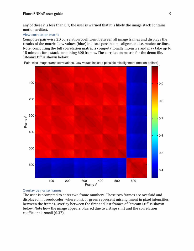
any of these r is less than 0.7, the user is warned that it is likely the image stack contains motion artifact. View correlation matrix Computes pair-‐wise 2D correlation coefficient between all image frames and displays the results of the matrix. Low values (blue) indicate possible misalignment, i.e. motion artifact. Note: computing the full correlation matrix is computationally intensive and may take up to 15 minutes for a stack containing 600 frames. The correlation matrix for the demo file, “steam1.tif” is shown below:

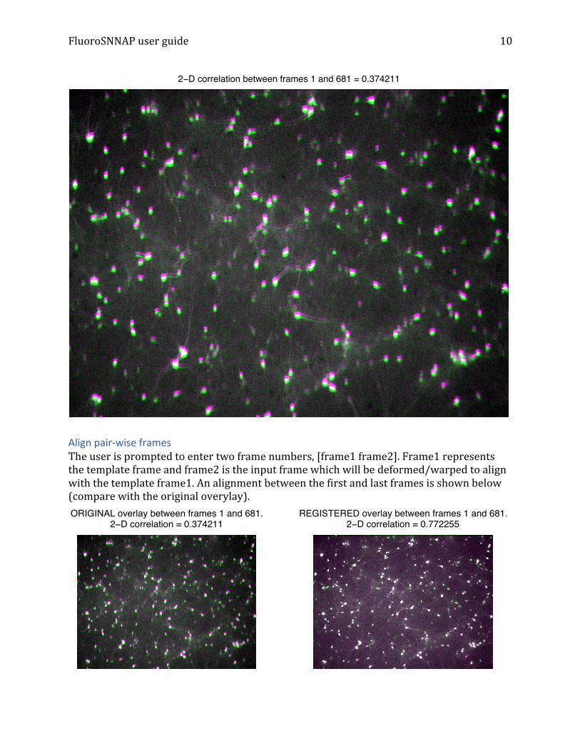
Overlay pair-‐wise frames: The user is prompted to enter two frame numbers. These two frames are overlaid and displayed in pseudocolor, where pink or green represent misalignment in pixel intensities between the frames. Overlay between the first and last frames of “stream1.tif” is shown below. Note how the image appears blurred due to a stage shift and the correlation coefficient is small (0.37).

Frame #

Fram

e #

Pair−wise image frame correlations. Low values indicate possible misalignment (motion artifact)

100 200 300 400 500 600

100

200

300

400

500

600

0.4

0.5

0.6

0.7

0.8

0.9

1


10

Align pair-‐wise frames The user is prompted to enter two frame numbers, [frame1 frame2]. Frame1 represents the template frame and frame2 is the input frame which will be deformed/warped to align with the template frame1. An alignment between the first and last frames is shown below (compare with the original overylay).

2−D correlation between frames 1 and 681 = 0.374211

ORIGINAL overlay between frames 1 and 681.2−D correlation = 0.374211

REGISTERED overlay between frames 1 and 681.2−D correlation = 0.772255


11

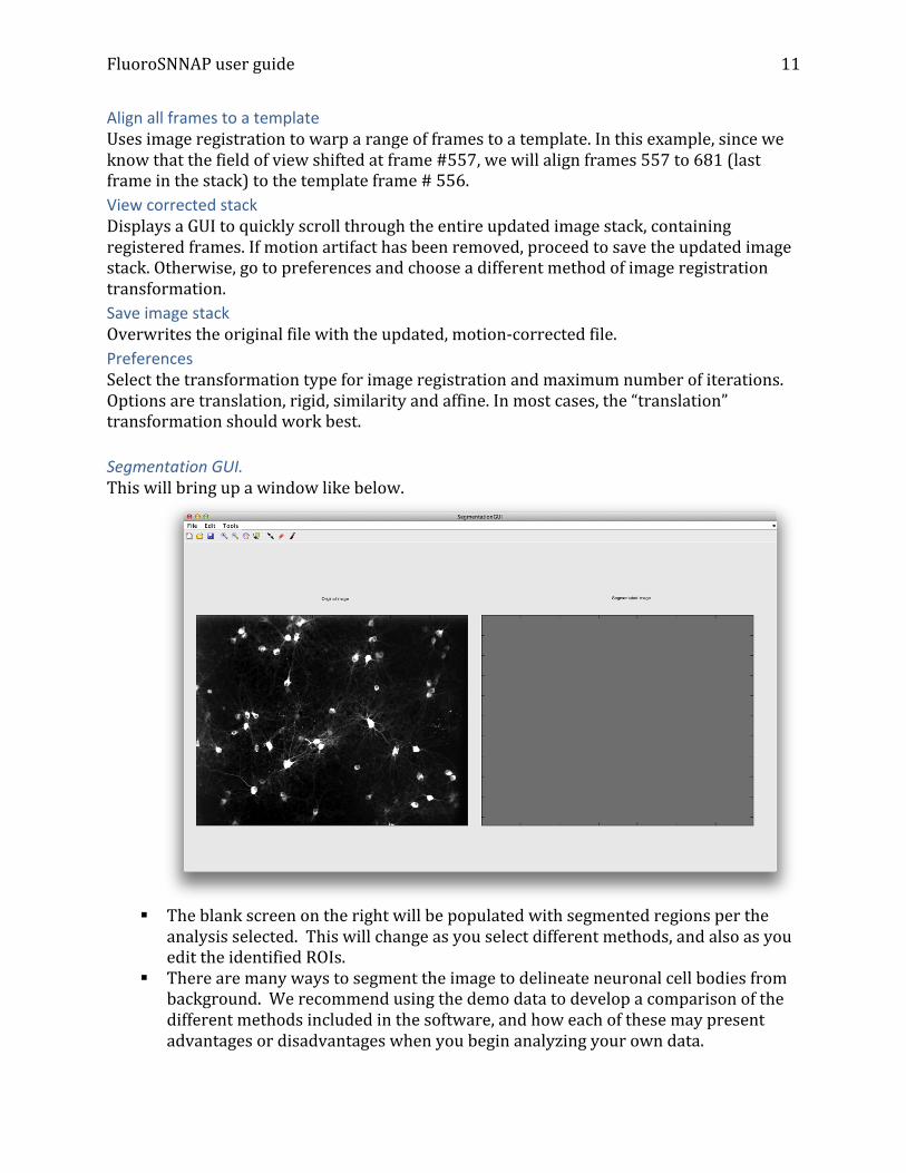
Align all frames to a template Uses image registration to warp a range of frames to a template. In this example, since we know that the field of view shifted at frame #557, we will align frames 557 to 681 (last frame in the stack) to the template frame # 556. View corrected stack Displays a GUI to quickly scroll through the entire updated image stack, containing registered frames. If motion artifact has been removed, proceed to save the updated image stack. Otherwise, go to preferences and choose a different method of image registration transformation. Save image stack Overwrites the original file with the updated, motion-‐corrected file. Preferences Select the transformation type for image registration and maximum number of iterations. Options are translation, rigid, similarity and affine. In most cases, the “translation” transformation should work best. Segmentation GUI. This will bring up a window like below.

§ The blank screen on the right will be populated with segmented regions per the

analysis selected. This will change as you select different methods, and also as you edit the identified ROIs.

§ There are many ways to segment the image to delineate neuronal cell bodies from background. We recommend using the demo data to develop a comparison of the different methods included in the software, and how each of these may present advantages or disadvantages when you begin analyzing your own data.


12

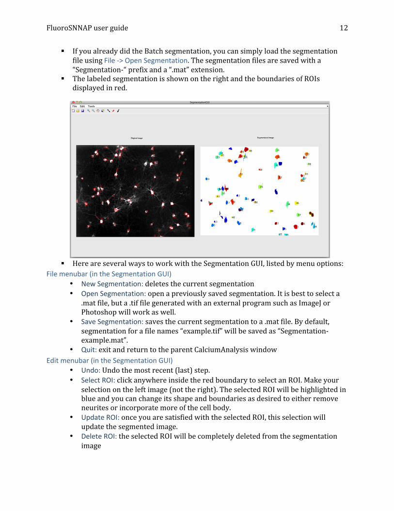
§ If you already did the Batch segmentation, you can simply load the segmentation file using File -‐> Open Segmentation. The segmentation files are saved with a “Segmentation-‐“ prefix and a “.mat” extension.

§ The labeled segmentation is shown on the right and the boundaries of ROIs displayed in red.

§ Here are several ways to work with the Segmentation GUI, listed by menu options:

File menubar (in the Segmentation GUI) • New Segmentation: deletes the current segmentation • Open Segmentation: open a previously saved segmentation. It is best to select a

.mat file, but a .tif file generated with an external program such as ImageJ or Photoshop will work as well.

• Save Segmentation: saves the current segmentation to a .mat file. By default, segmentation for a file names “example.tif” will be saved as “Segmentation-‐example.mat”.

• Quit: exit and return to the parent CalciumAnalysis window Edit menubar (in the Segmentation GUI)

• Undo: Undo the most recent (last) step. • Select ROI: click anywhere inside the red boundary to select an ROI. Make your

selection on the left image (not the right). The selected ROI will be highlighted in blue and you can change its shape and boundaries as desired to either remove neurites or incorporate more of the cell body.

• Update ROI: once you are satisfied with the selected ROI, this selection will update the segmented image.

• Delete ROI: the selected ROI will be completely deleted from the segmentation image


13

• Freehand delete: Select a region in the left image via freehand draw. Any objects within the freehand region will be removed from the segmented image. This is a great way to remove neurites without entirely deleting an ROI or to remove large portions of erroneously labeled segments.

• Remove neurites: As the name suggests, this option will remove neurites from the segmented image. For each labeled ROI, we compute a circularity factor, defined as 4*pi*area/perimeter^2. A perfectly circular ROI will have circularity factor = 1 and non-‐circles < 1. The user is prompted for a threshold value, default is 0.2. Any ROI whose circularity factor is less than 0.2 will be removed from the segmented image.

Tools menubar (in Segmentation GUI) • Threshold: Use the datatip to estimate backgroup intensity. Then enter a pixel

intensity threshold such that values > threshold are part of the foreground. Enter limits on minimum and maximum area of segmented objects. This is a very crude method of segmentation and will likely be a good start, although not the final product.

• Active contours Active contour segmentation is based on a method where you select a “seed” point within the ROI that you would like to segment. This seed point then grows until there is no further change in the image gradient at the contour. o Seed points: To use this tool, simply click anywhere within the cell body. You

can keep clicking as many cell bodies as you want. This function is in a continuous while loop.

o Stop: Once you are done, go to Tools -‐> Active contours -‐> Stop to exit out of the while loop and return.

• ICA: Automated segmentation using independent component analysis. This is the serial equivalent of “Batch segmentation” in the CalciumAnalysis figure. If you did not choose the Batch segmentation option, you can choose to do an ICA based segmentation using this tool. You will be prompted with a set of parameters. The default should work well in most cases. To enumerate the parameters: o Frames to process: range of frames to process. Default is to process all

frames in the image stack. Enter as [start_frame end_frame] o Number of principle components: The number of principle components to

derive. This value should be greater than the expected number of neurons in the field of view

o Number of PCs to use: Provide a list of principle components to retain for further analysis. This should be equal to or less than the number of principle components.

o Weight of temporal information: Enter a number between 0 and 1. 0 = pure spatial ICA, 1 = pure temporal ICA

o Number of independent components: This should be roughly the number of neurons in the field of view. More ICs will in general generate a better segmentation but will be slower in computation.


14

o Standard deviation of Gaussian smoothing kernel: Enter a value for smoothing the independent component filters.

o Threshold: Number of standard deviations above mean to threshold an object

o Min and max area: Enter as two element array, the minimum and maximum area of segmented objects

o Visualize processing: 0 = no, 1=yes. • Manual

o Set radius: enter a radius (in pixels) of neuronal cell body. This information will be used in the Tools -‐> Manual -‐> Ellipse callback.

o Ellipse: Click on the center of a neuronal cell body. This will place a circle of a preset radius (above tool) centered at the point selected. Continue to click and select more ROIs. To stop, select Tools -‐> Manual -‐> Stop.

o Freehand: Freehand draw an ROI. Use the zoom tools to better visualize the image.


15

View Segmentation § Displays the segmented image in separate figures.

Batch segmentation

§ Performs either active contour or ICA-‐based segmentation on each file within each folder listed in the left list box. ICA segmentation will take some time (15-‐ 30 minutes). This is equivalent to pressing the “Batch segmentation” button in the GUI.

Time-‐averaged image § Working file is the one selected in the right list box. This option will load the image

stack and compute the mean fluorescence of each pixel across time. Maximum projection

§ Working file is the one selected in the right list box. This option will load the image stack and compute the maximum projection image across time. That is, in the final image, a pixel at (i,j) will be the maximum of the set {(i,j) from frame 1, (i,j) from frame 2, …(i,j) from frame N}.


16

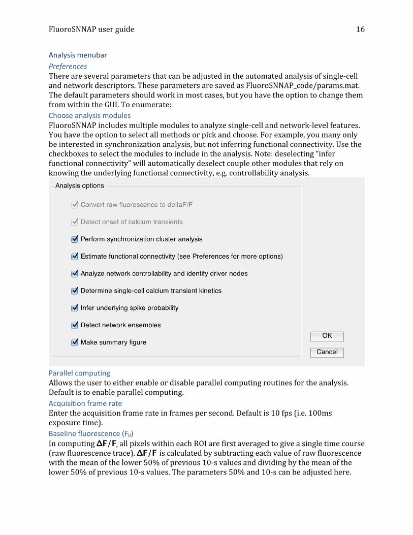
Analysis menubar Preferences There are several parameters that can be adjusted in the automated analysis of single-‐cell and network descriptors. These parameters are saved as FluoroSNNAP_code/params.mat. The default parameters should work in most cases, but you have the option to change them from within the GUI. To enumerate: Choose analysis modules FluoroSNNAP includes multiple modules to analyze single-‐cell and network-‐level features. You have the option to select all methods or pick and choose. For example, you many only be interested in synchronization analysis, but not inferring functional connectivity. Use the checkboxes to select the modules to include in the analysis. Note: deselecting “infer functional connectivity” will automatically deselect couple other modules that rely on knowing the underlying functional connectivity, e.g. controllability analysis.

Parallel computing Allows the user to either enable or disable parallel computing routines for the analysis. Default is to enable parallel computing. Acquisition frame rate Enter the acquisition frame rate in frames per second. Default is 10 fps (i.e. 100ms exposure time). Baseline fluorescence (F0) In computing ΔF/F, all pixels within each ROI are first averaged to give a single time course (raw fluorescence trace). ΔF/F is calculated by subtracting each value of raw fluorescence with the mean of the lower 50% of previous 10-‐s values and dividing by the mean of the lower 50% of previous 10-‐s values. The parameters 50% and 10-‐s can be adjusted here.


17

Calcium event detection • Template-‐based method is the default. This method compares a short moving

window of input fluorescence trace again a library of calcium transient waveforms. (provided with the source-‐code, spikes.mat) A similarity metric is computed and thresholded to determine whether the short input window “matches” a waveform in the library. Alternative option is based on fast spike deconvolution method.

• Calcium event detection threshold: threshold value above which a calcium event is detected. For template-‐based method, the threshold is a normalized correlation coefficient between a short input window and a calcium waveform from the library.

• Minimum deltaF/F0: The minimum change in fluorescence above baseline required for a putative event to be detected as a calcium transient.

Synchronization Analysis • Synchronization cluster analysis method: Several ways to determine

synchronization exist. Default is to determine instantaneous phase for each fluorescence trace and compute circular variance across pair-‐wise neurons. Other options are event and equal-‐time correlation. See references in accompanying manuscript for description. Lastly, the mutual information between pair-‐wise neuronal calcium fluorescence trace is inversely related to synchronization.

• Minimum size of synchronization cluster: Minimum number of neurons that make up a synchronized assembly

• Number of surrogate resampling: For statistical comparison, we use surrogate data to resample the calcium fluorescence trace (amplitude adjusted fourier transform). The number of times surrogate resampling is performed affects accuracy of the synchronization cluster analysis.

• Significance level: An alpha-‐level to determine functional connectivity. Functional connectivity We have implemented 5 different methods for inferring functional connectivity. They are, cross-‐correlation, partial-‐correlation, instantaneous phase, Granger causality and transfer entropy. Select which method you would like to use for inferring function connectivity using the drop-‐down menu. The appropriate panel of parameters will be highlighted in red. Refer to the View -‐> Functional connectivity section for more description of these methods. Cross-‐correlation: N resampling = number of times to reshuffle the dataset for statistical significance. Max time lag = time lag for cross-‐correlation, default is to compute normalized cross-‐correlation between pair-‐wise fluorescence traces between -‐0.5 to 0.5s time lag. Partial-‐correlation: alpha-‐level for significance Instantaneous phase: N sampling: number of times to resample for statistical significance (default 100), alpha-‐level for significance (default 0.001)


18

Granger causality: Max model order (default 20), alpha-‐level for significance (default 0.05), number of iterations: manually enter a number (100 default) or automatically determine (will take a very long time). Transfer entropy: N resampling (default 100): number of times to reshuffle to statistical significance, lags: default 1:10 Spike Inference ΔF/F trace is used to infer spike probability using the algorithms described in (Vogelstein, Packer et al. 2010). Parameters for inferring underlying spikes can be changed here. Network Ensemble Groups of statistically significant co-‐active neurons are determined by binarizing spike probability trace at 3 standard deviations and reshuffling active neurons 1000 times per (Miller, Ayzenshtat et al. 2014). Revert to default Reset all parameters to default values Process single file

§ Working file is the one selected in the right list box. This option will load the segmentation for the selected file and compute the mean fluorescence intensity for each ROI at each frame. Results are stored in a new matlab file in the same folder as the selected file. The raw fluorescence intensities are stored in a file prefixed by “CaSignal-‐“. In addition, the raw data is output to a comma delimited text file, where each row is an ROI and commas separate the mean fluorescence across frames.

§ Next, it will determine the onset of calcium transients using parameters set in Analysis -‐> Preferences.

§ Next, it will determine single cell calcium transient descriptors such as the onset of calcium transient, amplitude, rise and fall time.

§ Next, it will determine the level of synchronization in the calcium activity and infer a functional connectivity matrix using the method selected in Preferences.

§ Next, determine network ensembles § The results of this analysis are stored as a matlab .mat file and plain text .txt file.

Prefix “analysis-‐“ denotes the matlab .mat file and post-‐script _summary.txt denotes the plain text file. Also a summary figure is generated as .eps and .tiff files and stored in the directory “Figures”.

Batch single and network-‐analysis § This option batch processes all the files within each of the folder that have been

added to the list box on left. § Note, a segmentation file needs to exist for each tiff file to be processed. Run “Batch

Segmentation” if you don’t have segmentation files. § See above for description of the analysis.


19

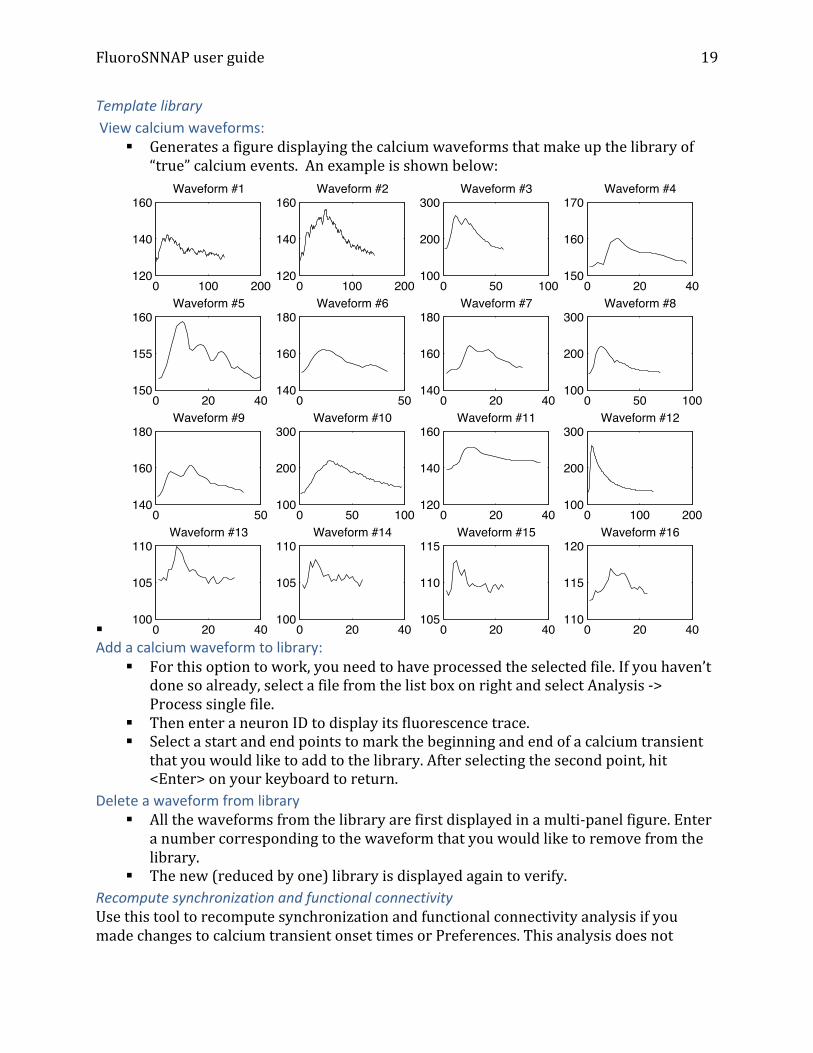
Template library View calcium waveforms:

§ Generates a figure displaying the calcium waveforms that make up the library of “true” calcium events. An example is shown below:

§ Add a calcium waveform to library:

§ For this option to work, you need to have processed the selected file. If you haven’t done so already, select a file from the list box on right and select Analysis -‐> Process single file.

§ Then enter a neuron ID to display its fluorescence trace. § Select a start and end points to mark the beginning and end of a calcium transient

that you would like to add to the library. After selecting the second point, hit <Enter> on your keyboard to return.

Delete a waveform from library § All the waveforms from the library are first displayed in a multi-‐panel figure. Enter

a number corresponding to the waveform that you would like to remove from the library.

§ The new (reduced by one) library is displayed again to verify. Recompute synchronization and functional connectivity Use this tool to recompute synchronization and functional connectivity analysis if you made changes to calcium transient onset times or Preferences. This analysis does not

0 100 200120

140

160Waveform #1

0 100 200120

140

160Waveform #2

0 50 100100

200

300Waveform #3

0 20 40150

160

170Waveform #4

0 20 40150

155

160Waveform #5

0 50140

160

180Waveform #6

0 20 40140

160

180Waveform #7

0 50 100100

200

300Waveform #8

0 50140

160

180Waveform #9

0 50 100100

200

300Waveform #10

0 20 40120

140

160Waveform #11

0 100 200100

200

300Waveform #12

0 20 40100

105

110Waveform #13

0 20 40100

105

110Waveform #14

0 20 40105

110

115Waveform #15

0 20 40110

115

120Waveform #16


20

require the use of original tiff stack so it can be useful to reanalyze or visualize pre-‐processed data.


21

View menubar: Use this menubar after you have done either single file or batch analysis. Make a filename selection before using this menubar.

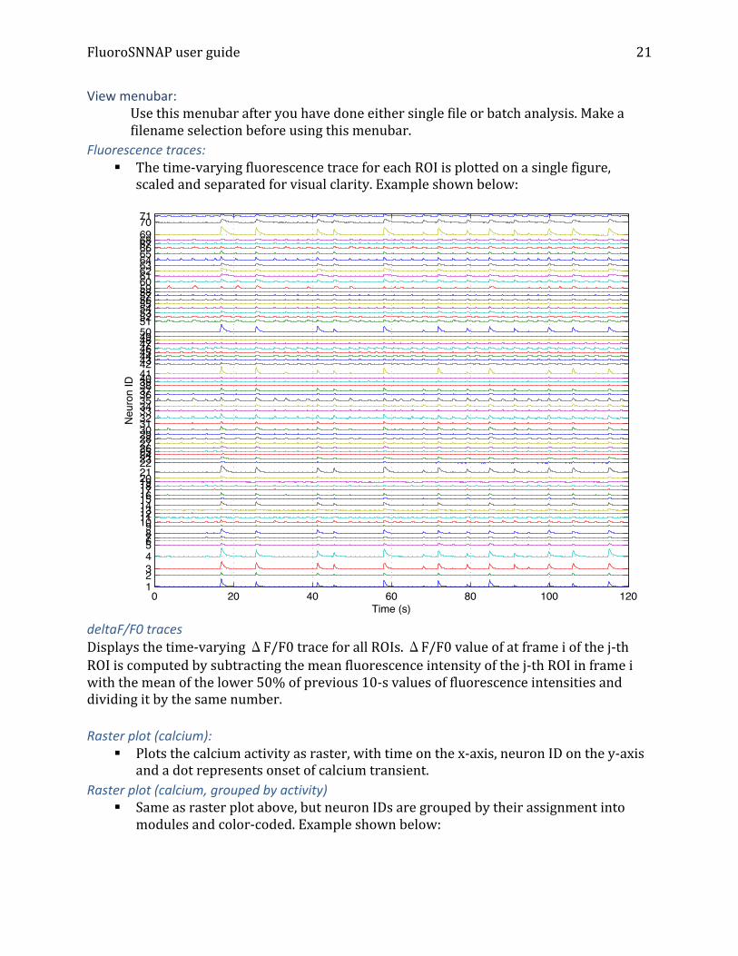
Fluorescence traces: § The time-‐varying fluorescence trace for each ROI is plotted on a single figure,

scaled and separated for visual clarity. Example shown below:

deltaF/F0 traces Displays the time-‐varying ΔF/F0 trace for all ROIs. ΔF/F0 value of at frame i of the j-‐th ROI is computed by subtracting the mean fluorescence intensity of the j-‐th ROI in frame i with the mean of the lower 50% of previous 10-‐s values of fluorescence intensities and dividing it by the same number. Raster plot (calcium):

§ Plots the calcium activity as raster, with time on the x-‐axis, neuron ID on the y-‐axis and a dot represents onset of calcium transient.

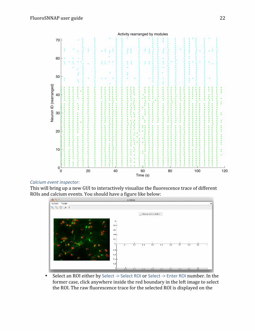
Raster plot (calcium, grouped by activity) § Same as raster plot above, but neuron IDs are grouped by their assignment into

modules and color-‐coded. Example shown below:

0 20 40 60 80 100 120123456789

1011121314151617181920212223242526272829303132333435363738394041424344454647484950515253545556575859606162636465666768697071

Time (s)

Neu

ron

ID


22

• Calcium event inspector: This will bring up a new GUI to interactively visualize the fluorescence trace of different ROIs and calcium events. You should have a figure like below:

• • Select an ROI either by Select -‐> Select ROI or Select -‐> Enter ROI number. In the

former case, click anywhere inside the red boundary in the left image to select the ROI. The raw fluorescence trace for the selected ROI is displayed on the

0 20 40 60 80 100 1200

10

20

30

40

50

60

70Activity rearranged by modules

Time (s)

Neu

ron

ID (r

earra

nged

)


23

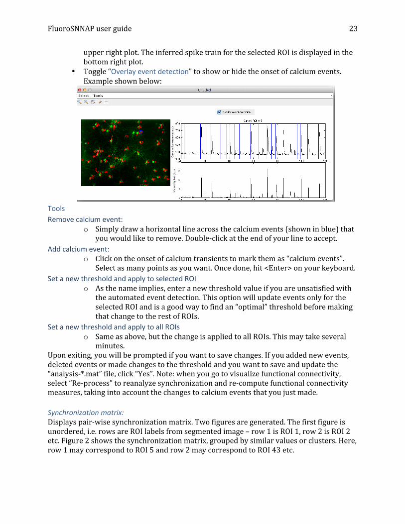
upper right plot. The inferred spike train for the selected ROI is displayed in the bottom right plot.

• Toggle “Overlay event detection” to show or hide the onset of calcium events. Example shown below:

• Tools Remove calcium event:

o Simply draw a horizontal line across the calcium events (shown in blue) that you would like to remove. Double-‐click at the end of your line to accept.

Add calcium event: o Click on the onset of calcium transients to mark them as “calcium events”.

Select as many points as you want. Once done, hit <Enter> on your keyboard. Set a new threshold and apply to selected ROI

o As the name implies, enter a new threshold value if you are unsatisfied with the automated event detection. This option will update events only for the selected ROI and is a good way to find an “optimal” threshold before making that change to the rest of ROIs.

Set a new threshold and apply to all ROIs o Same as above, but the change is applied to all ROIs. This may take several

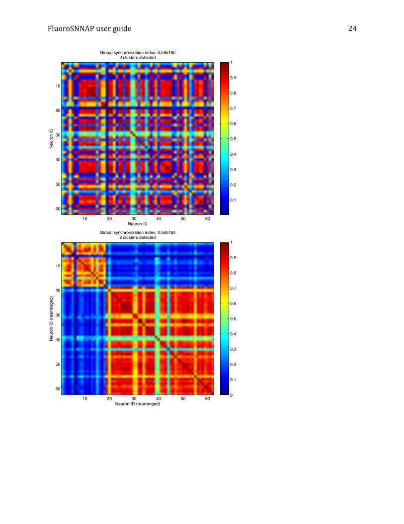
minutes. Upon exiting, you will be prompted if you want to save changes. If you added new events, deleted events or made changes to the threshold and you want to save and update the “analysis-‐*.mat” file, click “Yes”. Note: when you go to visualize functional connectivity, select “Re-‐process” to reanalyze synchronization and re-‐compute functional connectivity measures, taking into account the changes to calcium events that you just made. Synchronization matrix: Displays pair-‐wise synchronization matrix. Two figures are generated. The first figure is unordered, i.e. rows are ROI labels from segmented image – row 1 is ROI 1, row 2 is ROI 2 etc. Figure 2 shows the synchronization matrix, grouped by similar values or clusters. Here, row 1 may correspond to ROI 5 and row 2 may correspond to ROI 43 etc.


24

Neuron ID

Neu

ron

IDGlobal synchronization index: 0.565165

2 clusters detected

10 20 30 40 50 60

10

20

30

40

50

60

0.1

0.2

0.3

0.4

0.5

0.6

0.7

0.8

0.9

1

Neuron ID (rearranged)

Neu

ron

ID (r

earra

nged

)

Global synchronization index: 0.5651652 clusters detected

10 20 30 40 50 60

10

20

30

40

50

600

0.1

0.2

0.3

0.4

0.5

0.6

0.7

0.8

0.9

1


25

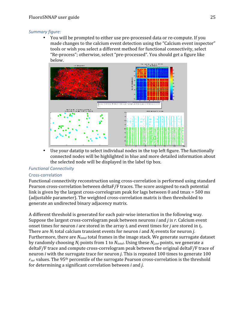
Summary figure: • You will be prompted to either use pre-‐processed data or re-‐compute. If you

made changes to the calcium event detection using the “Calcium event inspector” tools or wish you select a different method for functional connectivity, select “Re-‐process”; otherwise, select “pre-‐processed”. You should get a figure like below.

• • Use your datatip to select individual nodes in the top left figure. The functionally

connected nodes will be highlighted in blue and more detailed information about the selected node will be displayed in the label tip box.

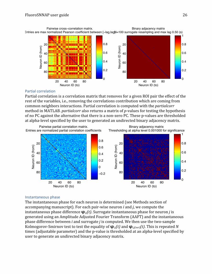
Functional Connectivity Cross-‐correlation Functional connectivity reconstruction using cross-‐correlation is performed using standard Pearson cross-‐correlation between deltaF/F traces. The score assigned to each potential link is given by the largest cross-‐correlogram peak for lags between 0 and tmax = 500 ms (adjustable parameter). The weighted cross-‐correlation matrix is then thresholded to generate an undirected binary adjacency matrix. A different threshold is generated for each pair-‐wise interaction in the following way. Suppose the largest cross-‐correlogram peak between neurons i and j is r. Calcium event onset times for neuron i are stored in the array ti and event times for j are stored in tj. There are Ni total calcium transient events for neuron i and Nj events for neuron j. Furthermore, there are Ntotal total frames in the image stack. We generate surrogate dataset by randomly choosing Nj points from 1 to Ntotal. Using these Nj,sur points, we generate a deltaF/F trace and compute cross-‐correlogram peak between the original deltaF/F trace of neuron i with the surrogate trace for neuron j. This is repeated 100 times to generate 100 rsur values. The 95th percentile of the surrogate Pearson cross-‐correlation is the threshold for determining a significant correlation between i and j.


26

Partial correlation Partial correlation is a correlation matrix that removes for a given ROI pair the effect of the rest of the variables, i.e., removing the correlations contribution which are coming from common neighbors interactions. Partial correlation is computed with the partialcorr method in MATLAB. partialcorr also returns a matrix of p-‐values for testing the hypothesis of no PC against the alternative that there is a non-‐zero PC. These p-‐values are thresholded at alpha-‐level specified by the user to generated an undirected binary adjacency matrix.

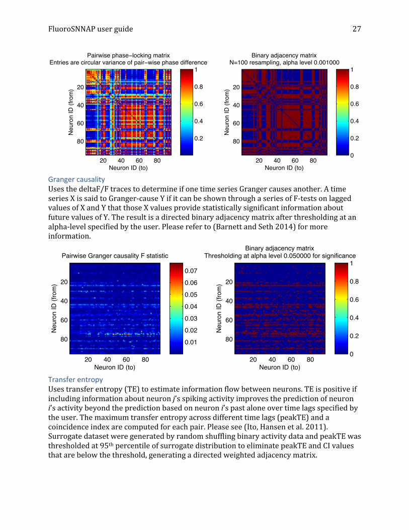
Instantaneous phase The instantaneous phase for each neuron is determined (see Methods section of accompanying manuscript). For each pair-‐wise neuron i and j, we compute the instantaneous phase difference φi,j(t). Surrogate instantaneous phase for neuron j is generated using an Amplitude Adjusted Fourier Transform (AAFT) and the instantaneous phase difference between i and surrogate j is computed. We then use the two-‐sample Kolmogorov-‐Smirnov test to test the equality of φi,j(t) and φi,j(sur)(t). This is repeated N times (adjustable parameter) and the p-‐value is thresholded at an alpha-‐level specified by user to generate an undirected binary adjacency matrix.

Neuron ID (to)

Ne

uro

n I

D (

fro

m)

Pairwise cross−correlation matrix.Entries are max normalized Pearson coefficient between [−lag,lag]

20 40 60 80

20

40

60

80

0

0.2

0.4

0.6

0.8

Neuron ID (to)

Ne

uro

n I

D (

fro

m)

Binary adjacency matrixN=100 surrogate resampling and max lag 0.50 (s)

20 40 60 80

20

40

60

80

0

0.2

0.4

0.6

0.8

1

Neuron ID (to)

Neu

ron

ID (f

rom

)

Pairwise partial correlation matrix.Entries are normalized partial correlation coefficients

20 40 60 80

20

40

60

80 −0.2

0

0.2

0.4

0.6

0.8

Neuron ID (to)

Neu

ron

ID (f

rom

)

Binary adjacency matrixThresholding at alpha level 0.001000 for significance

20 40 60 80

20

40

60

80

0

0.2

0.4

0.6

0.8

1


27

Granger causality Uses the deltaF/F traces to determine if one time series Granger causes another. A time series X is said to Granger-‐cause Y if it can be shown through a series of F-‐tests on lagged values of X and Y that those X values provide statistically significant information about future values of Y. The result is a directed binary adjacency matrix after thresholding at an alpha-‐level specified by the user. Please refer to (Barnett and Seth 2014) for more information.

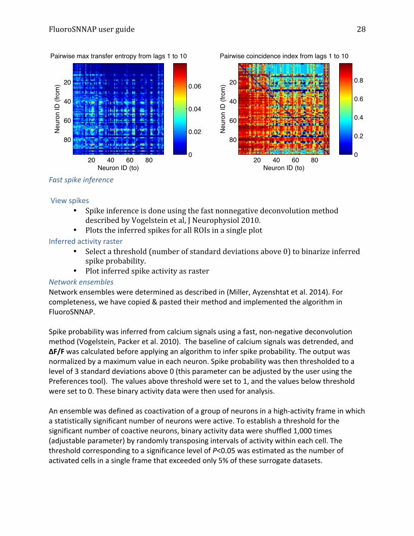
Transfer entropy Uses transfer entropy (TE) to estimate information flow between neurons. TE is positive if including information about neuron j’s spiking activity improves the prediction of neuron i’s activity beyond the prediction based on neuron i’s past alone over time lags specified by the user. The maximum transfer entropy across different time lags (peakTE) and a coincidence index are computed for each pair. Please see (Ito, Hansen et al. 2011). Surrogate dataset were generated by random shuffling binary activity data and peakTE was thresholded at 95th percentile of surrogate distribution to eliminate peakTE and CI values that are below the threshold, generating a directed weighted adjacency matrix.

Neuron ID (to)

Ne

uro

n I

D (

fro

m)

Pairwise phase−locking matrixEntries are circular variance of pair−wise phase difference

20 40 60 80

20

40

60

80 0.2

0.4

0.6

0.8

1

Neuron ID (to)

Ne

uro

n I

D (

fro

m)

Binary adjacency matrixN=100 resampling, alpha level 0.001000

20 40 60 80

20

40

60

80

0

0.2

0.4

0.6

0.8

1

Neuron ID (to)

Neu

ron

ID (f

rom

)

Pairwise Granger causality F statistic

20 40 60 80

20

40

60

80 0.01

0.02

0.03

0.04

0.05

0.06

0.07

Neuron ID (to)

Neu

ron

ID (f

rom

)

Binary adjacency matrixThresholding at alpha level 0.050000 for significance

20 40 60 80

20

40

60

80

0

0.2

0.4

0.6

0.8

1


28

Fast spike inference View spikes

• Spike inference is done using the fast nonnegative deconvolution method described by Vogelstein et al, J Neurophysiol 2010.

• Plots the inferred spikes for all ROIs in a single plot Inferred activity raster

• Select a threshold (number of standard deviations above 0) to binarize inferred spike probability.

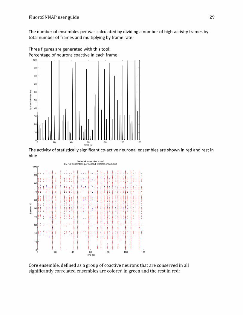
• Plot inferred spike activity as raster Network ensembles Network ensembles were determined as described in (Miller, Ayzenshtat et al. 2014). For completeness, we have copied & pasted their method and implemented the algorithm in FluoroSNNAP. Spike probability was inferred from calcium signals using a fast, non-‐negative deconvolution method (Vogelstein, Packer et al. 2010). The baseline of calcium signals was detrended, and ΔF/F was calculated before applying an algorithm to infer spike probability. The output was normalized by a maximum value in each neuron. Spike probability was then thresholded to a level of 3 standard deviations above 0 (this parameter can be adjusted by the user using the Preferences tool). The values above threshold were set to 1, and the values below threshold were set to 0. These binary activity data were then used for analysis. An ensemble was defined as coactivation of a group of neurons in a high-‐activity frame in which a statistically significant number of neurons were active. To establish a threshold for the significant number of coactive neurons, binary activity data were shuffled 1,000 times (adjustable parameter) by randomly transposing intervals of activity within each cell. The threshold corresponding to a significance level of P<0.05 was estimated as the number of activated cells in a single frame that exceeded only 5% of these surrogate datasets.

Neuron ID (to)

Neu

ron

ID (f

rom

)Pairwise max transfer entropy from lags 1 to 10

20 40 60 80

20

40

60

80

0

0.02

0.04

0.06

Neuron ID (to)

Neu

ron

ID (f

rom

)

Pairwise coincidence index from lags 1 to 10

20 40 60 80

20

40

60

80

0

0.2

0.4

0.6

0.8


29

The number of ensembles per was calculated by dividing a number of high-‐activity frames by total number of frames and multiplying by frame rate. Three figures are generated with this tool: Percentage of neurons coactive in each frame:

The activity of statistically significant co-‐active neuronal ensembles are shown in red and rest in blue.

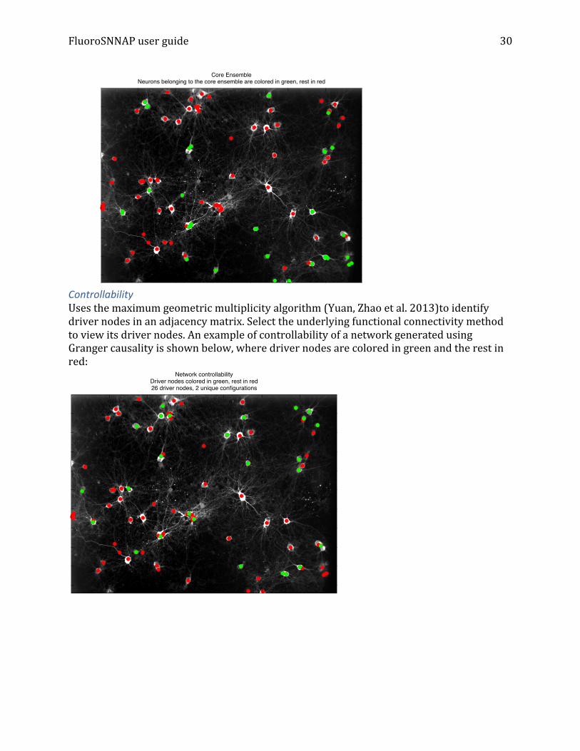
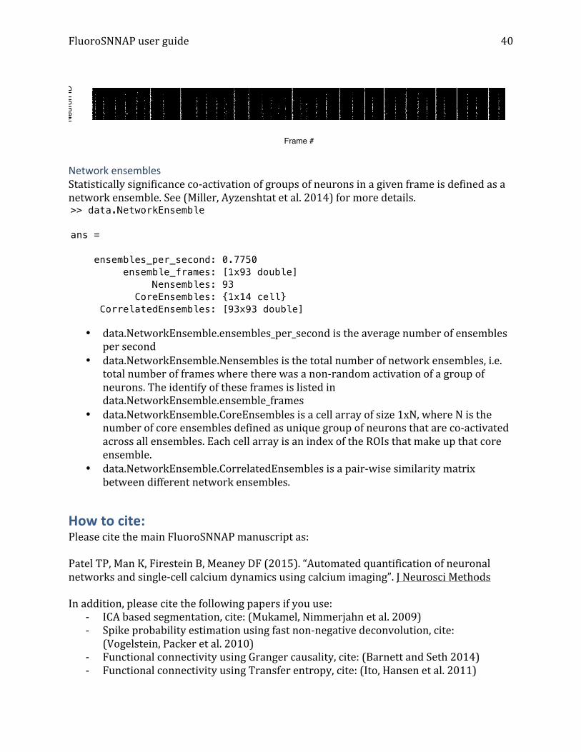
Core ensemble, defined as a group of coactive neurons that are conserved in all significantly correlated ensembles are colored in green and the rest in red:

0 20 40 60 80 100 1200

10

20

30

40

50

60

70

80

90

100

Time (s)

% o

f cel

ls c

o−ac

tive

0 20 40 60 80 100 1200

10

20

30

40

50

60

70

80

90

100

Time (s)

Neu

ron

ID

Network ensemles in red0.7750 ensembles per second, 93 total ensembles


30

Controllability Uses the maximum geometric multiplicity algorithm (Yuan, Zhao et al. 2013)to identify driver nodes in an adjacency matrix. Select the underlying functional connectivity method to view its driver nodes. An example of controllability of a network generated using Granger causality is shown below, where driver nodes are colored in green and the rest in red:

Core EnsembleNeurons belonging to the core ensemble are colored in green, rest in red

Network controllabilityDriver nodes colored in green, rest in red26 driver nodes, 2 unique configurations


31

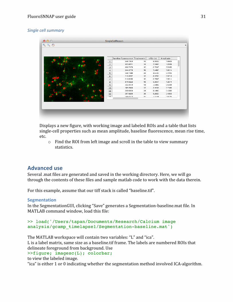
Single cell summary

Displays a new figure, with working image and labeled ROIs and a table that lists single-‐cell properties such as mean amplitude, baseline fluorescence, mean rise time, etc.

o Find the ROI from left image and scroll in the table to view summary statistics.

Advanced use Several .mat files are generated and saved in the working directory. Here, we will go through the contents of these files and sample matlab code to work with the data therein. For this example, assume that our tiff stack is called “baseline.tif”.

Segmentation In the SegmentationGUI, clicking “Save” generates a Segmentation-‐baseline.mat file. In MATLAB command window, load this file: >> load('/Users/tapan/Documents/Research/Calcium image analysis/gcamp_timelapse1/Segmentation-baseline.mat') The MATLAB workspace will contain two variables: “L” and “ica”. L is a label matrix, same size as a baseline.tif frame. The labels are numbered ROIs that delineate foreground from background. Use >>figure; imagesc(L); colorbar; to view the labeled image. “ica” is either 1 or 0 indicating whether the segmentation method involved ICA-‐algorithm.


32

To use your own segmentation file with the FluoroSNNAP GUI, for example a segmentation generated using ImageJ or Photoshop, simply load the segmented image into MATLAB. Suppose this image is called Mask.tif. >> I = imread(‘Mask.tif’); % load the image >> L = bwlabel(I~=0); % label the image >> ica = 0; % no ICA algorithm was used Save the workspace as Segmentation-‐baseline.mat

CaSignal A CaSignal-‐baseline.mat is generated which contains the raw fluorescence vs. frame data for each ROI. Load this file and you should have a variable “analysis”. This is a structure containing fields: >> analysis analysis = image: [520x696x3 uint16] filename: '/Users/tapan/Documents/Research/Calcium image analysis/gcamp_timelapse1/base...' F_cell: [95x1200 double] F_whole: [1200x1 double] L: [520x696 double] fps: 10 The dot operator references fields of a structure.

• analysis.image is the time-‐averaged image frame. To view it, >> figure; imshow(analysis.image,[]);

• analysis.F_cell is a matrix of size ROIs x frames. Entries are mean fluorescence

intensity within the ROI. To see the fluorescence trace for ROI 5, >> figure; plot(analysis.F_cell(5,:));

• analysis.F_whole is full frame mean fluorescence. • analysis.L is the label matrix. ROIs labeled in L index the rows in F_cell. To view the

labeled image, >> figure; imagesc(analysis.L);

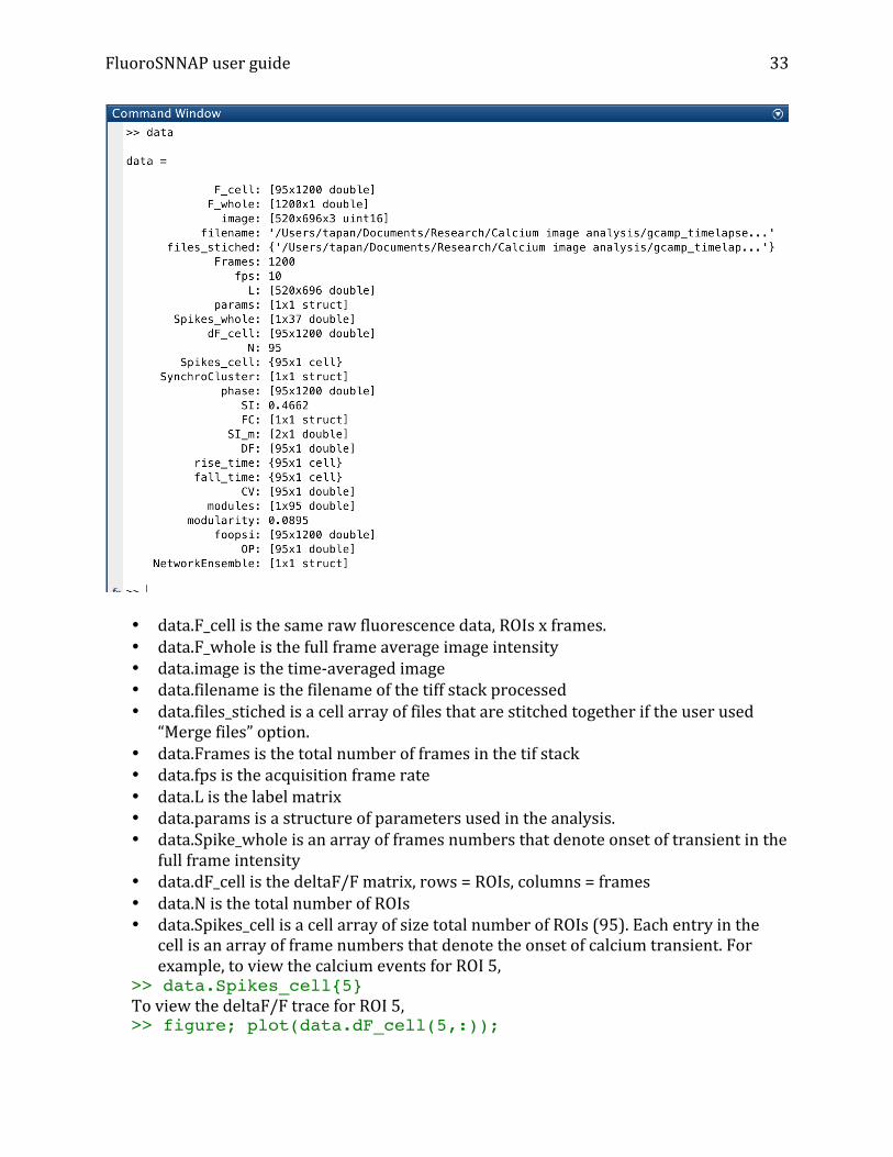
Analysis An analysis-‐baseline.mat is generated and contains all single-‐cell and network level analysis. Load this file and you should have a “data” variable in your workspace.


33

• data.F_cell is the same raw fluorescence data, ROIs x frames. • data.F_whole is the full frame average image intensity • data.image is the time-‐averaged image • data.filename is the filename of the tiff stack processed • data.files_stiched is a cell array of files that are stitched together if the user used

“Merge files” option. • data.Frames is the total number of frames in the tif stack • data.fps is the acquisition frame rate • data.L is the label matrix • data.params is a structure of parameters used in the analysis. • data.Spike_whole is an array of frames numbers that denote onset of transient in the

full frame intensity • data.dF_cell is the deltaF/F matrix, rows = ROIs, columns = frames • data.N is the total number of ROIs • data.Spikes_cell is a cell array of size total number of ROIs (95). Each entry in the

cell is an array of frame numbers that denote the onset of calcium transient. For example, to view the calcium events for ROI 5,

>> data.Spikes_cell{5} To view the deltaF/F trace for ROI 5, >> figure; plot(data.dF_cell(5,:));


34

To see the calcium events overlaid on the deltaF/F trace, >> OverlaySpikes(data.dF_cell(5,:), data.Spikes_cell{5});

Synchronization

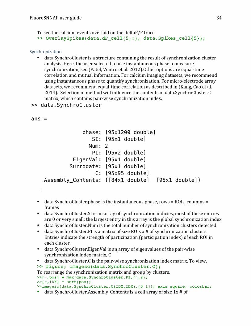
• data.SynchroCluster is a structure containing the result of synchronization cluster analysis. Here, the user selected to use instantaneous phase to measure synchronization, see (Patel, Ventre et al. 2012).Other options are equal-‐time correlation and mutual information. For calcium imaging datasets, we recommend using instantaneous phase to quantify synchronization. For micro-‐electrode array datasets, we recommend equal-‐time correlation as described in (Kang, Cao et al. 2014). Selection of method will influence the contents of data.SynchroCluster.C matrix, which contains pair-‐wise synchronization index.

• data.SynchroCluster.phase is the instantaneous phase, rows = ROIs, columns = frames

• data.SynchroCluster.SI is an array of synchronization indicies, most of these entries are 0 or very small; the largest entry in this array is the global synchronization index

• data.SynchroCluster.Num is the total number of synchronization clusters detected • data.SynchroCluster.PI is a matrix of size ROIs x # of synchronization clusters.

Entries indicate the strength of participation (participation index) of each ROI in each cluster.

• data.SynchroCluster.EigenVal is an array of eigenvalues of the pair-‐wise synchronization index matrix, C

• data.SynchroCluster.C is the pair-‐wise synchronization index matrix. To view, >> figure; imagesc(data.SynchroCluster.C); To rearrange the synchronization matrix and group by clusters, >>[~,pos] = max(data.SynchroCluster.PI,[],2); >>[~,IDX] = sort(pos); >>imagesc(data.SynchroCluster.C(IDX,IDX),[0 1]); axis square; colorbar; • data.SynchroCluster.Assembly_Contents is a cell array of size 1x # of


35

synchronization clusters. Contents of this cell array are the ROI numbers that participate in the synchronization cluster. One neuron may participate in more than 1 cluster

• data.phase is an instantaneous phase matrix of size ROIs x frames • data.SI is the global synchronization index. • data.SI_m is the synchronization index per module. The community structure

(modules) is determined from an underlying adjacency matrix (see below) and synchronization of neurons within each module is computed. If the user selects to compute functional connectivity using all 5 methods, this routine will default to using the adjacency matrix derived from instantaneous phase.

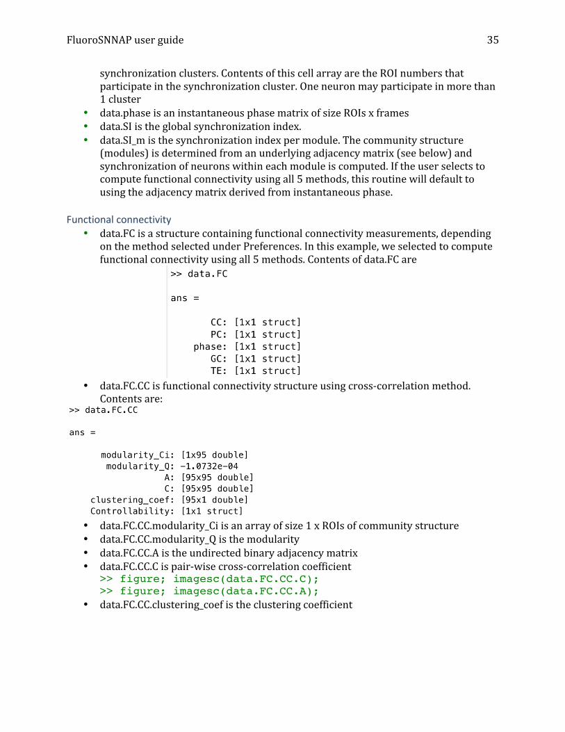
Functional connectivity

• data.FC is a structure containing functional connectivity measurements, depending on the method selected under Preferences. In this example, we selected to compute functional connectivity using all 5 methods. Contents of data.FC are

• data.FC.CC is functional connectivity structure using cross-‐correlation method.

Contents are:

• data.FC.CC.modularity_Ci is an array of size 1 x ROIs of community structure • data.FC.CC.modularity_Q is the modularity • data.FC.CC.A is the undirected binary adjacency matrix • data.FC.CC.C is pair-‐wise cross-‐correlation coefficient

>> figure; imagesc(data.FC.CC.C); >> figure; imagesc(data.FC.CC.A);

• data.FC.CC.clustering_coef is the clustering coefficient


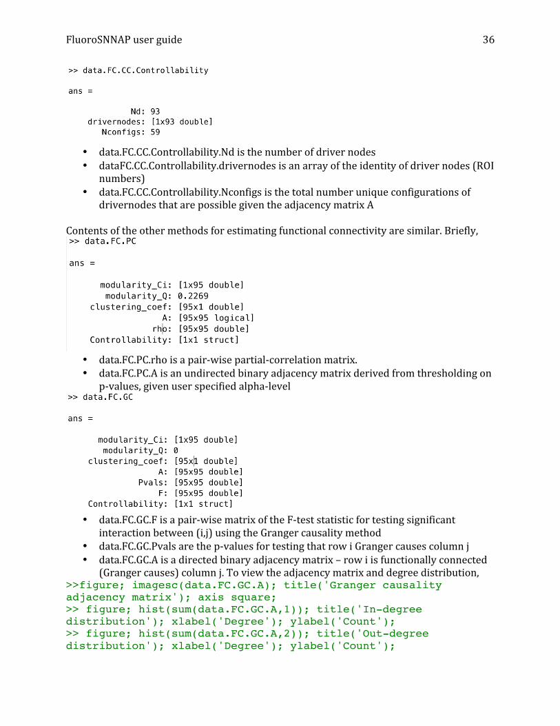
36

• data.FC.CC.Controllability.Nd is the number of driver nodes • dataFC.CC.Controllability.drivernodes is an array of the identity of driver nodes (ROI

numbers) • data.FC.CC.Controllability.Nconfigs is the total number unique configurations of

drivernodes that are possible given the adjacency matrix A Contents of the other methods for estimating functional connectivity are similar. Briefly,

• data.FC.PC.rho is a pair-‐wise partial-‐correlation matrix. • data.FC.PC.A is an undirected binary adjacency matrix derived from thresholding on

p-‐values, given user specified alpha-‐level

• data.FC.GC.F is a pair-‐wise matrix of the F-‐test statistic for testing significant

interaction between (i,j) using the Granger causality method • data.FC.GC.Pvals are the p-‐values for testing that row i Granger causes column j • data.FC.GC.A is a directed binary adjacency matrix – row i is functionally connected

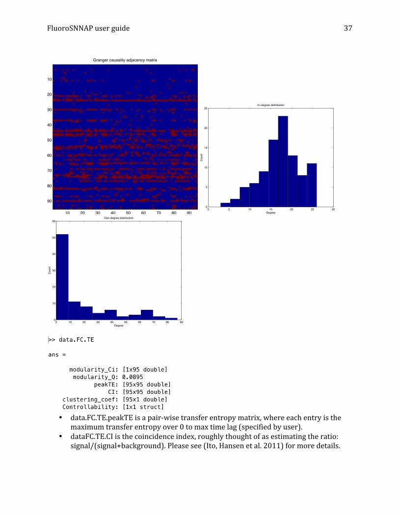
(Granger causes) column j. To view the adjacency matrix and degree distribution, >>figure; imagesc(data.FC.GC.A); title('Granger causality adjacency matrix'); axis square; >> figure; hist(sum(data.FC.GC.A,1)); title('In-degree distribution'); xlabel('Degree'); ylabel('Count'); >> figure; hist(sum(data.FC.GC.A,2)); title('Out-degree distribution'); xlabel('Degree'); ylabel('Count');


37

• data.FC.TE.peakTE is a pair-‐wise transfer entropy matrix, where each entry is the

maximum transfer entropy over 0 to max time lag (specified by user). • dataFC.TE.CI is the coincidence index, roughly thought of as estimating the ratio:

signal/(signal+background). Please see (Ito, Hansen et al. 2011) for more details.

Granger causality adjacency matrix

10 20 30 40 50 60 70 80 90

10

20

30

40

50

60

70

80

90

0 5 10 15 20 25 300

5

10

15

20

25In−degree distribution

Degree

Cou

nt

0 10 20 30 40 50 60 70 80 900

10

20

30

40

50

60Out−degree distribution

Degree

Cou

nt


38

Single-‐cell descriptors For each neuron, the kinetics of calcium transients (amplitude, rise time, fall time) are computed. And the average across all events in a given neuron is reported along with 95% confidence intervals.

• data.DF is an Nx1 array, where entries are the average amplitude (as ΔF/F) per neuron.

• data.CV is an Nx1 array, whose entries are the coefficient of variation in amplitude of calcium transients

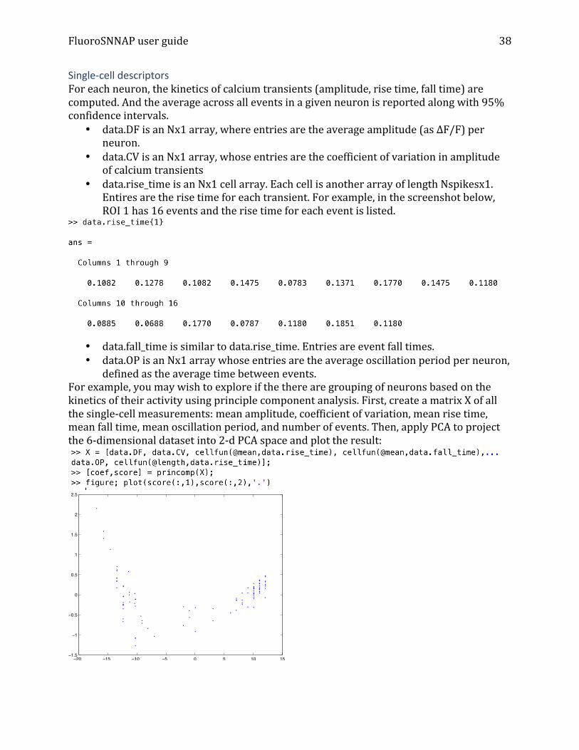
• data.rise_time is an Nx1 cell array. Each cell is another array of length Nspikesx1. Entires are the rise time for each transient. For example, in the screenshot below, ROI 1 has 16 events and the rise time for each event is listed.

• data.fall_time is similar to data.rise_time. Entries are event fall times. • data.OP is an Nx1 array whose entries are the average oscillation period per neuron,

defined as the average time between events. For example, you may wish to explore if the there are grouping of neurons based on the kinetics of their activity using principle component analysis. First, create a matrix X of all the single-‐cell measurements: mean amplitude, coefficient of variation, mean rise time, mean fall time, mean oscillation period, and number of events. Then, apply PCA to project the 6-‐dimensional dataset into 2-‐d PCA space and plot the result:

−20 −15 −10 −5 0 5 10 15

−1.5

−1

−0.5

0

0.5

1

1.5

2

2.5


39

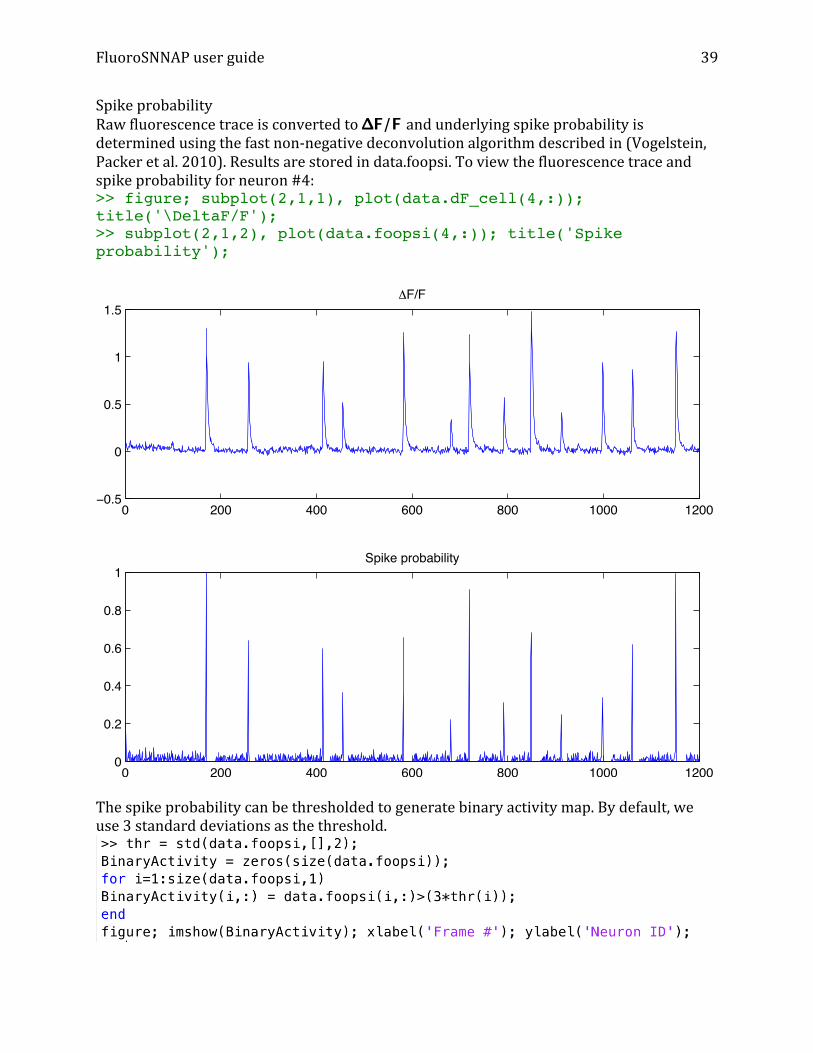
Spike probability Raw fluorescence trace is converted to ΔF/F and underlying spike probability is determined using the fast non-‐negative deconvolution algorithm described in (Vogelstein, Packer et al. 2010). Results are stored in data.foopsi. To view the fluorescence trace and spike probability for neuron #4: >> figure; subplot(2,1,1), plot(data.dF_cell(4,:)); title('\DeltaF/F'); >> subplot(2,1,2), plot(data.foopsi(4,:)); title('Spike probability');

The spike probability can be thresholded to generate binary activity map. By default, we use 3 standard deviations as the threshold.

0 200 400 600 800 1000 1200−0.5

0

0.5

1

1.56F/F

0 200 400 600 800 1000 12000

0.2

0.4

0.6

0.8

1Spike probability


40

Network ensembles Statistically significance co-‐activation of groups of neurons in a given frame is defined as a network ensemble. See (Miller, Ayzenshtat et al. 2014) for more details.

• data.NetworkEnsemble.ensembles_per_second is the average number of ensembles

per second • data.NetworkEnsemble.Nensembles is the total number of network ensembles, i.e.

total number of frames where there was a non-‐random activation of a group of neurons. The identify of these frames is listed in data.NetworkEnsemble.ensemble_frames

• data.NetworkEnsemble.CoreEnsembles is a cell array of size 1xN, where N is the number of core ensembles defined as unique group of neurons that are co-‐activated across all ensembles. Each cell array is an index of the ROIs that make up that core ensemble.

• data.NetworkEnsemble.CorrelatedEnsembles is a pair-‐wise similarity matrix between different network ensembles.

How to cite: Please cite the main FluoroSNNAP manuscript as: Patel TP, Man K, Firestein B, Meaney DF (2015). “Automated quantification of neuronal networks and single-‐cell calcium dynamics using calcium imaging”. J Neurosci Methods In addition, please cite the following papers if you use:

-‐ ICA based segmentation, cite: (Mukamel, Nimmerjahn et al. 2009) -‐ Spike probability estimation using fast non-‐negative deconvolution, cite:

(Vogelstein, Packer et al. 2010) -‐ Functional connectivity using Granger causality, cite: (Barnett and Seth 2014) -‐ Functional connectivity using Transfer entropy, cite: (Ito, Hansen et al. 2011)

Frame #

Neu

ron

ID


41

References:

Barnett, L. and A. K. Seth (2014). "The MVGC multivariate Granger causality toolbox: a new approach to Granger-‐causal inference." J Neurosci Methods 223: 50-‐68. Ito, S., M. E. Hansen, R. Heiland, A. Lumsdaine, A. M. Litke and J. M. Beggs (2011). "Extending transfer entropy improves identification of effective connectivity in a spiking cortical network model." PLoS One 6(11): e27431. Kang, W. H., W. Cao, O. Graudejus, T. Patel, S. Wagner, D. Meaney and B. Morrison Iii, 3rd (2014). "Alterations in Hippocampal Network Activity after In Vitro Traumatic Brain Injury." J Neurotrauma. Miller, J. E., I. Ayzenshtat, L. Carrillo-‐Reid and R. Yuste (2014). "Visual stimuli recruit intrinsically generated cortical ensembles." Proc Natl Acad Sci U S A 111(38): E4053-‐4061. Mukamel, E. A., A. Nimmerjahn and M. J. Schnitzer (2009). "Automated analysis of cellular signals from large-‐scale calcium imaging data." Neuron 63(6): 747-‐760. Patel, T. P., S. C. Ventre and D. F. Meaney (2012). "Dynamic changes in neural circuit topology following mild mechanical injury in vitro." Ann Biomed Eng 40(1): 23-‐36. Vogelstein, J. T., A. M. Packer, T. A. Machado, T. Sippy, B. Babadi, R. Yuste and L. Paninski (2010). "Fast nonnegative deconvolution for spike train inference from population calcium imaging." J Neurophysiol 104(6): 3691-‐3704. Yuan, Z., C. Zhao, Z. Di, W. X. Wang and Y. C. Lai (2013). "Exact controllability of complex networks." Nat Commun 4: 2447.