Journal of Propulsion and PowerVol. ??, No. ?, Month??–Month?? year??

Fluorescence visualisation of the hypersonic flowestablishment over a blunt fin

J. S. Fox∗, S. O’Byrne†, A. F. P. Houwing‡, A. Papinniemi§,P. M. Danehy¶, N. R. Mudford‖

Aerophysics and Laser-based Diagnostics Research LaboratoryDepartment of Physics and Theoretical Physics

Australian National UniversityActon, A.C.T. 0200, AUSTRALIA

Fluorescence imaging is used to investigate the separated flow upstream of a blunt fin in ahypersonic free-stream with a transitional boundary layer. Images are presented to show the flowdevelopment before, during and after the test time of the free-piston shock tunnel used to generatethe flow. These images indicate that the test time in this facility is long enough to achieve a steadyflow over the blunt fin. Thermocouple measurements are included to compare the surface heat fluxupstream of the fin with that for flow along a flat plate with the same free-stream conditions. Theheat flux results are consistent with separation in a transitional boundary layer and show that theseparated flow is oscillatory.

Nomenclaturea Sound speed, m.s−1

aδ Average sound speed in boundary layer, m.s−1

d Fin diameter, md1 Separation length, mh1 Verticle distance from plate to triple point, mh2 Vertical distance from plate to shear layer below triple point, mhe Specific enthalpy of free-stream, J.kg−1

hw Specific enthalpy at wall, J.kg−1

lsep. Separation length, mppitot,∞ Pitot pressure, Pap0 Nozzle reservoir pressure, Pa•qs(t) Surface heat flux, J.m−2.s−1

t Time, sue Velocity of freestream, m.s−1

x Distance from nozzle throat along nozzle axis, m

Cf Skin friction coefficientL Length of flat plate, mM Mach numberM∞ Mach number in freestreamPr Prandtl numberR Gas constant, J/(kg.K)Re Reynolds numberSt Stanton number based on free-stream conditionsT Temperature, KT∞ Temperature in freestream, KT ∗ Eckert reference temperature, KTw Temperature at wall, KU∞ Flow speed ahead of the bow shock, m.s−1

U Velocity, m.s−1

X Position at which ∆tNT is evaluated, m

∗Graduate Student, Student Member AIAA†Graduate Student, Student Member AIAA‡Associate Professor, Member AIAA§Graduate Student, Department of Aerospace and Mechanical En-

gineering, University College, University of New South Wales, Camp-bell, A.C.T. 2612, AUSTRALIA

¶Research Scientist, Member AIAA, Instrumentation Systems De-velopment Branch, MS 236, NASA Langley Research Center, Hamp-ton, VA 23681-2199, USA

‖Senior Lecturer, Member AIAA, Department of Aerospace andMechanical Engineering, University College, University of New SouthWales, Campbell, A.C.T. 2612, AUSTRALIA

Received Month. day, year; revision Month. day, year; accepted forpublication Month. day, year. Copyright c© year by the American Insti-tute of Aeronautics and Astronautics, Inc. No copyright is asserted inthe United States under Title 17, U.S. Code. The U.S. Government has aroyalty-free license to exercise all rights under the copyright claimed hereinfor Governmental Purposes. All other rights are reserved by the copyrightowner.

α1 Angle of separation shock with horizontal, degα2 Angle of shear layer with horizontal, degαλ Angle of lambda shock with horizontal, degγ Ratio of specific heatsγ∞ Ratio of specific heats in freestreamρ∞ Density ahead of bow shock, kg.m3

ρe Density of freestream, kg.m3

ρs Density behind bow shock, kg.m3

τb.l. Characteristic response time (boundary layer), sτsep. Characteristic response time (separated flow), sτb.s. Characteristic response time (bow shock), s

∆ Asymptotic value of shock stand-off distance, m∆′ Shock stand-off distance when established, m∆tnozzle Time to establish nozzle flow, s∆tE Time to establish overall flow, s∆tE,max Maximum time to establish overall flow, s∆tE,min Minimum time to establish overall flow, s∆tNT Time for sound waves to travel through nozzle, s

Introduction

AERODYNAMIC heating is one of the critical problemsin the design of high speed aerospace vehicles. High

thermal stresses occur in vehicles around the nose region, onleading edges and in corner regions, such as in the junctionsbetween wing and body, fin and body, pylon and wing, finand wing, and, flap and wing. In addition, the intake ductsof air-breathing engines can be subject to high thermal loadsresulting from shock-shock and shock-vortex interactions.A number of important viscous interaction problem regionshave been identified:1,2 leading-edge shock impingement; fininteraction; flap deflection; axial corner flows; and a numberof other shock-wave/boundary-layer interaction problems.This paper investigates one of these problems, the fin in-terference problem, in which a shock wave-boundary layerinteraction induces flow separation.

Figure 1 shows the main features of hypersonic flow over ablunt-fin on a flat plate. The bow shock upstream of the fingenerates a pressure rise which is communicated upstreamthrough the subsonic portion of the boundary layer, causingthe flow on the flat plate to separate and deflect away fromthe fin. Stollery2 has discussed the flow features in the three-dimensional flow-field near an unswept blunt-nosed strut (orblunt fin). The primary flow feature associated with the di-version of flow around the fin is a horseshoe vortex,3,4 whichforms upstream of the fin. Theory predicts the presence of

1

2 FOX ET AL: FLOW ESTABLISHMENT OVER A BLUNT FIN

������

����������������������������

����

��������������������������������������������

Supersonic jetimpinging on front face of

blunt fin. Regionof high

pressure and surface heat flux.

Inner vortex

Region of highpressure and

surface heat flux.

Horseshoe vortexSeparation

Line

Leading edge shockLaser sheetRegion imaged

by camera

To computer

ICCDCamera

��������

Separation shock

Lambda shock

Fig. 1 Schematic of the three-dimensional flow arounda blunt fin (after Stollery 1987).

∆

α1 α2

αλ

Fig. 2 Side-view schematic of the blunt fin attached to aflat plate with the expected flow features and positionsof the thermocouples. The blunt fin is 323 mm fromthe leading edge of the flat plate; thermocouples TC1,TC2, TC3 and TC4 are 113, 170, 274, and 307 mm,respectively from the leading edge.

two vortices in this model of the flow, but as many as sixvortices have been indicated by surface oil patterns in somecases.5 In experiments, maximum pressures and heat fluxrates occur near the reattachment lines associated with thesevortices.3

The problems associated with attempting to visualise thefin interaction flows are twofold. Firstly, optical accessfor traditional line-of-sight visualisation techniques, suchas shadowgraph, schlieren, or interferometry, is severelyrestricted by the presence of the surfaces that make upthe fin-body junction. Secondly, even if optical access isachieved, line-of-sight methods, which are strictly suitablefor two-dimensional flows only, will not be able to resolvethe highly three-dimensional features.

To date, the flow-field structure for this type of flowhas been inferred largely from surface gauge measurementsor surface visualisation techniques such as the sublimationmethod; oil flow techniques; the laser interferometer skinfriction technique; infra-red thermography; and liquid crys-tal thermography.6–10 Flow-field visualisation, other thanline-of-sight visualisation, has been restricted to the elec-tron beam method11 which is confined to low density flows,and planar laser scattering12 requiring seeding with parti-cles, which may lag behind fluid particles in their motion.

The restrictions of optical access and the problems associ-ated with the visualisation of a three-dimensional flow-fieldcan be overcome by using planar laser-induced fluorescence(PLIF). PLIF can provide comprehensive flow-field visu-alisation of the supersonic fin interaction flow as well asvaluable information against which theoretical models andcomputational fluid dynamics (CFD) calculations can betested.13 At present, CFD rarely predicts the complex flowscreated by the interaction between boundary layers, separa-tion shocks, reattachment shocks, free shear layers and otherflow features accurately.14–16 Using PLIF visualisation, theposition and shape of these flow features can be determinedexperimentally, thus providing simple parameters, such as

the location of the separation point and the angle of theseparation shock, which can be directly compared to CFDcalculations.

This paper describes a series of PLIF flow visualisationand heat flux measurements that determine whether the sep-arated flow upstream of a blunt-fin model geometry reachesa steady state during the test time available in a free-piston shock tunnel.17 Free-piston shock tunnels are pulsedfacilities that can be used to generate a wide range of hy-personic flow conditions. A major difficulty associated withtheir use is their extremely short flow duration. This prob-lem becomes particularly serious when examining separatedflows, such as in the blunt fin problem, because the timerequired for flow to establish in the separated region is sig-nificantly longer than the other flow features of interest suchas bow shocks and attached boundary layers. The steadyflow test-time in such a facility is the time interval betweenthe establishment of steady test-gas flow in the nozzle andthe arrival of the driver gas. Depending on the conditionsrequired in the test section, the test time can range from100 µs to 4 ms. Previous work using PLIF visualisation18

has shown that a steady flow in the near-wake of a conecan be achieved during the test time available to a smallfree-piston shock tunnel.

Flow establishmentFor the purposes of the following discussion, we define

∆tnozzle as the time taken to establish steady nozzle flow atthe model station together with time constants τb.l., τsep.,and τb.s., which are the characteristic times for response ofthe boundary layer, separated flow and bow shock on theblunt fin, respectively, to changes in the free stream flow.These characteristic times may be evaluated as the timestaken for each flow feature to reach its steady state afterimpulsive exposure of a body to a steady freestream flow.As will be discussed below, the literature contains empir-ical expressions for evaluating these times. The questionto be addressed, then, is at what time, ∆tE, after incidentprimary shock reflection, does the model flow become sta-tionary? Here, the term stationary is used in the same senseas in turbulence studies - that is, although flow quantitiesmay fluctuate over the short term, their long term meansare constant.

Mallinson et al.19 stated that a conservative estimate of∆tE in a compression corner may be obtained as the sumof ∆tnozzle, τb.l., and τsep.. This estimate assumes thatthe flow features develop serially. The conservative natureof this assumption derives from the fact that, in reality, allof the flow features will need to respond to flow changesthat occur while the nozzle flow is being established andthat interactions between the inviscid flow, boundary layerand separated region may continue sometime after the noz-zle flow has established. An additional contributor to theconservative margin is the division of the separated flow intoboundary layer, separated flow region and bow shock. Werethe combination to be considered as a single flow featurethen it would have a single characteristic time appropriateto the simultaneous development of the three individual fea-tures as discerned here. However, following Mallinson, wetake the sum of ∆tnozzle, τb.l., τsep., and τb.s. as a usefulupper limit for flow establishment time. That is,

∆tE,max = ∆tnozzle + τb.l. + τsep. + τb.s. (1)

In the case where all of τb.l., τsep., and τb.s. are much lessthan ∆tnozzle, we may argue that the boundary layer, sep-arated flow region and bow shock respond quickly enough tofreestream flow changes to allow us to make the approxima-tion that the nozzle establishment time is a useful minimumfor the flow establishment time. That is,

∆tE,min ≈ ∆tnozzle (2)

FOX ET AL: FLOW ESTABLISHMENT OVER A BLUNT FIN 3

Position in flow x ∆tNT ∆tnozzle τb.l. τb.s. τsep. ∆tE,min ∆tE,max(mm) (µs) (µs) (µs) (µs) (µs) (µs) (µs)

Leading edge of plate 870 305 1450 401 40 226 1450 2117

Exit of nozzle 1030 359 1500 404 40 228 1500 2172

Blunt fin model 1195 419 1560 399 40 230 1560 2229

Table 1 Calculated establishment times for flow processes, calculated for three different positions in the flow.

We now proceed to find approximations for ∆tnozzle,τb.l., τsep., and τb.s., for the present flow, in order to deter-mine values for ∆tE,max and ∆tE,min, plus examine thereasonableness of this last approximation.

Nozzle flow establishmentThe starting process in a supersonic nozzle has been stud-

ied extensively in previous work.20,21 It is initiated whenthe primary incident shock in the shock tube is reflected atthe shock tube end wall and the first test gas passes intothe nozzle. Much of the earlier work on nozzle flow es-tablishment deals with planar two-dimensional nozzle flows.However, the qualitative features of the axisymmetric caseare expected to be similar. From this early work, the nozzleflow evolution is known to be a complicated process involv-ing multiple shock and boundary layer interactions.21 Infact, it is so complicated, that it is well nigh impossible toquantify ∆tnozzle on the basis of fluid mechanical theory.Consequently, ∆tnozzle is determined experimentally here,as described below.

For a perfect gas flow, the test section flow can be con-sidered to be steady when the Mach number of the flowis constant. Boyce et al22 argue that the Mach number issteady in flows with changing nozzle reservoir pressure, p0,when the ratio of the free-stream pitot pressure ppitot,∞(t)at a time t to the nozzle reservoir pressure p0(t−∆tNT) atan earlier time t−∆tNT is constant. Here the nozzle transittime, ∆tNT, is the time taken for acoustic disturbances totravel from the nozzle reservoir to the test section:

∆tNT =

x=X∫x=0

dx

U + a(3)

Here x is the distance from the throat along the nozzle cen-treline, X is the position at which ∆tNT is evaluated, Uis the local flow velocity and is a the local speed of sound.The parameters U and a can be calculated using the one-dimensional non-equilibrium nozzle code STUBE.23

Additionally, in the case of steady nozzle flow of a perfectgas,

ppitot, ∞ (t)

p0(t−∆tNT

) =

[1 +

2γ

γ + 1

(M2 − 1

)] −1γ−1

[(γ + 1) M2

(γ − 1) M2 + 2

] γγ−1

(4)

where M is the Mach number of the flow just upstream ofthe pitot probe and γ is the ratio of the specific heats. Hencethe ratio of the pitot and nozzle reservoir pressures can alsobe used to give an indication of the Mach number of the flowat any given time after shock reflection, if γ is known. Thenozzle flow behaves as if γ is close to 1.4, consistent withthe fact that this is a low enthalpy flow condition. However,the bow shock generated around the pitot probe elevates thetemperature, which decreases the effective γ to about 1.33.Hence, γ = 1.33 is used in this equation.

Establishment of steady attached boundary layer flowDavies and Bernstein24 found that the characteristic time

to achieve a steady attached boundary layer on a flat plate,

τb.l., is given by

τb.l. =3.33L

U∞(5)

where L is the length of the flat plate and U∞ is the free-stream flow velocity.

Establishment of steady shear layer downstream ofseparation

The characteristic time to establish a separated flow on acompression corner, τsep., was calculated by Holden25 using

τsep. =lsep.aδ

=d1

aδ(6)

where lsep. is the separation length (d1 in our work), andaδ is the average sound speed in the boundary layer. Wewill assume that this equation can be also used for the char-acteristic time to establish the separated flow produced onthe blunt fin. The assumption underlying this formulationis that the dimensions and flow within the separated flowregion are set by means of an acoustic wave which emanatesfrom the fin and travels forward to the steady flow sepa-ration point. The average speed of sound in the boundarylayer, aδ, can be determined using an intermediate temper-ature such as the Eckert temperature T ∗,26 where

T ∗ = 0.5(Tw + T∞) + 0.11(Pr)1/2(γ∞ − 1)M2∞T∞ (7)

Here Tw is the wall temperature, assumed to be 300 K, T∞is the free-stream temperature, Pr is the Prandtl number,assumed to have a value of 0.72, γ∞ is the free-stream ra-tio of specific heats which, for these experiments, is closeto a value of 1.4, and is M the free-stream Mach number.Assuming ideal-gas behaviour, aδ can be written as:

aδ =√

γ∞RT ∗ (8)

where R is the gas constant.In this work, we estimate the length of the separation

region from the flow visualisation by extrapolating the sep-aration shock to the point at which it would intersect theflat plate and measuring the distance from that point to thecorner of the blunt fin. This method has been used in aprevious schlieren visualisation study of turbulent blunt finflow.27 Other flow parameters required for the calculationof are determined from the computer code STUBE,23 usedto calculate the steady nozzle flow.

Establishment time for bow shockMiles et al.28 derived the following equation for the time

to establish a bow shock at the front of a circular cylinder:

τb.s. =∆

U∞

(ρs

ρ∞− 1

)ln

(1− ∆′

∆

)−1

(9)

where U∞ is the flow speed ahead of the bow shock, ∆ is theasymptotic value of the shock stand-off distance, ∆′ is thevalue of the shock stand-off distance when the bow shock isconsidered to be established, ρ∞ is the density ahead of thebow shock, and ρs is the density behind the bow shock. Inour work, we will consider the bow shock to be established

4 FOX ET AL: FLOW ESTABLISHMENT OVER A BLUNT FIN

when the stand-off distance has reached 95 % of its asymp-totic value. That is, ∆′/∆ = 0.95. In the case of perfect gasflow over a cylinder of diameter d, mass flux considerationsand experimental data show that ∆ is given by the followingformula:29

∆d

= 1.16ρ∞ρS

(10)

Experimental methodFlow conditions

Experiments were performed in the T3 free-piston shocktunnel at the Australian National University.17 A 305-mmexit-diameter axi-symmetric conical nozzle with a 35-mmdiameter throat and 7.5-degree internal half-angle was usedto expand gas at a stagnation temperature and pressure of3480 K and 15.9 MPa, respectively, over a blunt fin modelmounted on the centreline of a flat plate. Because of theconical geometry of the nozzle, the free-stream flow can beapproximated as a source flow. A slight flow divergencecauses the Mach number of the free-stream to vary from avalue of approximately 6.1 at the leading edge of the flatplate to 6.9 at the location of the blunt fin.

The shock tube fill condition of 2% O2 in N2, selectedto generate the required amount of NO for good fluores-cence imaging, results in a test gas composition of 1.6% NO,1.2% O2, 0.06% O and 97.14% N2 by mole-fraction at thenozzle exit (calculated using the computer code STUBE23).The Mach number, temperature, and pressure of the free-stream were 6.4 ±0.1, 446 ±5 K, 7.2 ±0.4 kPa respectively;the stagnation enthalpy was 3.90 ±0.02 MJ/kg. The unitReynolds number at these conditions is 5.9 × 106 m−1.Based on previous work,30 we assume a transition Reynoldsnumber of 1.0 × 106, which indicates that transition shouldoccur approximately 170 mm from the leading edge of theflat plate, that is, 155 mm, or 3.9 fin diameters, upstreamof the fin.

Model and instrumentation

The flat plate is shown schematically in Fig. 2. It wasmounted on a sting positioned so that the top surface wasin the centre of the nozzle flow. The blunt fin was attachedperpendicularly to the flat plate; it was not swept and wasat a zero angle of attack. Before the experiment, the leadingedge of the flat plate was inserted 160 mm inside the nozzlesuch that the fin was 163 mm downstream of the nozzleexit. During the experiment, the shock tunnel recoils byabout 30 mm away from the model. The blunt fin is 38 mmthick with a hemi-cylindrical nose. The height of the bluntfin was 100 mm, which is high enough to be considered assemi-infinite, so that any increases in height of the blunt finwould not affect the flow.

Co-axial chromel-alumel thermocouples, of 2.3-mm outerdiameter, were used to obtain the heat flux measurements.Four of these were flush-mounted along the centre-line of theplate, at the positions indicated in Fig. 2. For the remain-der of the discussion, the thermocouples are labelled TC1through TC4, in order of increasing distance downstream ofthe leading edge of the plate. They were placed so that TC1was in the undisturbed flat plate boundary-layer flow, TC2was located near the separation point, while TC3 and TC4were within the separated region, and within the area illu-minated by the laser sheet. The blunt fin is 323 mm fromthe leading edge of the flat plate, whereas thermocouplesTC1, TC2, TC3 and TC4 are 113, 170, 274, and 307 mm,respectively from the leading edge.

The thermocouples were produced in-house and have beenused successfully in previous measurements performed for ahypersonic compression-corner flow.19 Although less sensi-tive than thin-film gauges, thermocouples are less suscep-tible to damage arising from diaphragm fragments or thehigh levels of heat flux that can occur just upstream of thefin. The thermocouple voltages were amplified using a 30-dB differential pre-amplifier and recorded by two Tektronix

TDS 310 digital oscilloscopes.

Pitot and nozzle reservoir pressure measurements

Prior to the blunt fin experiments, the flow conditionswere characterised by measuring the pitot pressure at theexit of the nozzle and comparing it with the nozzle reservoirpressure as described above. The pitot probe was placed atthe exit of the nozzle and along the centreline of the flow.

PLIF excitation and detection

The PLIF method is a well-established flow imaging tech-nique that can be used to measure static temperature,31pressure,32 perform species imaging,33,34 and for flow vi-sualisation.18 In the current work, we used the R2(13.5)transition in the A2Σ← X2Π(0, 0) band of NO, determinedfrom previous work35 to be a good transition for qualita-tively visualising the important flow features. A sheet oflaser light tuned to this transition illuminated the plane ofsymmetry illustrated in Figs 1 and 2. The resultant fluo-rescence from laser-excited NO molecules in the illuminatedplane was imaged by an intensified CCD camera as shownin Fig. 1. Luminosity from flow contaminants36 reduces thesignal to noise ratio and for that reason we used a shortcamera gate of approximately 100 ns. This gate was longenough to capture over 90% of the fluorescence while shortenough to reject the majority of the natural flow luminosity.A more detailed description of the optical setup is providedby Fox et al.33

ResultsThe results of the calculations for the establishment time

of different flow processes at the leading edge of the flatplate, the exit of the nozzle and at the blunt fin model areshown in Table 1. The characteristic times of the establish-ment of bow shock, separated region and boundary layerare, indeed, significantly smaller than ∆tnozzle, which in-dicates we may be justified in making the approximation∆tE = ∆tE,min = ∆tnozzle.

Determination of nozzle flow start up time

The result of the calculation for the ratio of pitot pressureto nozzle reservoir pressure is shown in Fig. 3 with thenozzle reservoir and pitot pressure traces. A constant valueis reached at about 1.5 ms, which agrees well with resultsfrom previous work,22 and is consistent with a perfect gasflow having a Mach number of 6.4 and an effective value of1.33 for the ratio of specific heats.

∆∞

∞

Fig. 3 Nozzle reservior pressure trace and free-streampitot pressure trace shown with the ratio of pitot toreservoir pressures at this 4 MJ/kg condition. The timewhen steady nozzle flow was established is the time whenthis pressure ratio first becomes constant.

FOX ET AL: FLOW ESTABLISHMENT OVER A BLUNT FIN 5

Fig. 4 Planar laser-induced fluorescence images of the flow development: a) 250 µs, b) 400 µs, c) 600 µs, d) 800 µs,e) 1400 µs, f) 1600 µs, g) 1800 µs, h) 3180 µs, and i) 4660 µs. Flow feature identified by letters: n.s.l. – nozzle shearlayer; b.s. – bow shock; s.l. – shear layer; l.s.s. – large-scale structure; s.s. – separation shock; e.s. – embedded shock;s.i. – shock-shock interaction; l.s. – lambda shock; and j. – jet produced by shock-shock interaction.

PLIF imaging of flow development

Figure 4 shows PLIF images, corrected for spatial varia-tion in the profile of the laser sheet, taken at different delaytimes and shows how the flow develops. Each image is ob-tained during successive runs of the tunnel and thereforethe images will be subject to some variation due to the non-repeatability of the turbulent structures. The datum for alltimes is the time of the reflection of the primary incidentshock in the shock tube. In all images the flow is from leftto right and the laser enters from the top of the image. Eachimage is 75 ±1 mm wide and 55 ±1 mm high. The rightedge of each image corresponds to the position of the bluntfin. The images are displayed in grayscale using a logarith-mic scale, with light shades corresponding to high signalsand dark shades to low signals.

Some features of the nozzle start-up processes are seenin Fig. 4 (a) at a time of 250 µs. The nozzle startingshock is apparent as a sudden change in intensity near thefin. This feature is similar to that reported in the schlierenimages of Smith.20 In this image, the nozzle shear layer(n.s.l.) is visible, indicating that the nozzle flow is not yetestablished. At a later time of 400 µs, as shown in Fig. 4(b), the flow begins to show the presence of the separationshock. However, the bow shock is still not properly formedand the shear layer appears laminar. At the top of theimage the nozzle shear layer is still visible. As seen by the

disturbance in the bow shock near the top of the blunt fin,the bow shock appears to interact with the nozzle shear layerin some way at a time of 600 µs (see Fig. 4 (c)). At thistime, turbulent structures become visible in the separatedregion. The separation-shock/bow-shock interaction is nowstrong enough to form a lambda shock. Between 400 and800 µs (see Figs. 4 (b) - (d)), the separation point movesdownstream until, by 800 µs, it is within the field of view.The bow shock appears to be steady from 800 µs onwardsbut the separated flow region does not reach a steady stateuntil much later.

The images in Figs 4(e)–(g) are typical of images observedin the time interval from 1.4 to 3.0 ms. They are charac-terised by a steady bow shock (b.s.), however the separationshock (s.s.) shape is slightly different from shot to shot.Variations in its shape are attributed to embedded shockwaves (e.s.), which are produced by supersonic flow deflectedby turbulent eddies in the shear layer (s.l.). The locationand size of these turbulent eddies vary from shot to shot,thereby varying the location and strength of the embeddedshocks. Consequently, the interaction of these shocks withthe separation shock result in shot-to-shot variations in itsshape. Figure 4(g) shows a particularly large scale structure(l.s.s.), which was observed at a delay time of 1800 µs. Theappearance of such structures occurs randomly at differentdelay times.

6 FOX ET AL: FLOW ESTABLISHMENT OVER A BLUNT FIN

After about 3.0 ms, the PLIF images become progres-sively darker with delay time as a result of diminishing NOconcentration due to contamination and thus dilution by thedriver gas. Further evidence of driver gas contaminationat these delay times is the increase in the shock standoffdistance, consistent with the accompanying increase in theratio of specific heats.

Figures 5 to 8 show the various parameters defined in Fig.2 measured from the PLIF images as a function of delaytime. All distances are normalised to the fin diameter, d,of 38 mm and all angles are measured in degrees from theplate surface.

Variation of the normalised bow shock stand-off distance,∆/d, with time is shown in Fig. 5. Both the minimumand maximum distance of the bow shock from the fin wererecorded. This was considered necessary because the bowshock was not perfectly vertical in some of the images takenat earlier delays (see, for example, the bow shock shape ata time of 400 µs). The inviscid flow associated with thebow shock above the interaction region appears to stabilisesafter about 800 µs. The bow-shock stand-off distance takesless time than other flow features to reach a steady valuebecause it is an inviscid feature of the flow. According toEq. 9, it takes only about 40 µs for the bow shock to es-tablish on the fin at these conditions. Furthermore, at highMach numbers, and in the absence of chemical effects, theshock stand-off distance is only a weak function of Machnumber. Hence, in the later stages of the nozzle flow estab-lishment, it is quite insensitive to Mach number changes.If we assume that the measurements of the pitot pressureprovide a good indication of the free-stream Mach numberduring these later stages, the Mach number changes fromabout 5.9 at 800 µs to about 6.4 at 1500 µs. Based onEq. 10 and the dependence of the density ratio on Machnumber, the normalised shock stand off distance ∆/d willchange by only a small amount. In fact, according to Eq. 10,it will change from 0.193 to 0.189 fin diameters over thisMach number range. The small change of 0.004 fin diam-eters is smaller than the uncertainty in our measurementsand hence we expect the stand-off distance to appear con-stant after 800 µs. This explains why the shock on the bluntfin appears to stabilise well before the flow at the exit of thenozzle has reached a constant Mach number. After about3 ms the bow shock stand-off distance slowly increases asthe gas composition of the flow changes due to the arrival ofthe driver gas. This increase in shock stand-off distance isconsistent with the dependence ∆/d of on the density ratioacross the shock. The density ratio in turn depends on γ,which increases when the monatonic driver gas arrives.

∆min

/d ∆max

/d∆

µ

Fig. 5 Minimum and maximum bow-shock stand-offdistances from the blunt fin normalised to blunt fin di-ameter. The shock stand-off distance appears to stabiliseat about 800 µs.

h1/d

α1

α

(µs)

(µs)

Fig. 6 a) The height from the flat plate to the point ofinteraction between the separation shock and the bowshock, and the angle of the separation shock to the flatplate, and b) the distance from the blunt fin to the pointof intersection of the separation shock on the flat plate.All these parameters appear steady from ≈ 1.5 – 3.0 msfrom shock reflection, giving some indication of when theinviscid interactions are stable.

Figure 6 (a) shows how the vertical distance, h1, from theplate to the point of interaction between the bow and sep-aration shocks and the angle of the separation shock, α1,changes with delay time. The point at which the separa-tion shock intersects the flat plate occurs just outside theregion of the PLIF images. An estimate of the separationlength d1, the distance from the blunt fin to the point wherethe boundary layer separates from the flat plate, can be ob-tained by extrapolating the separation shock to the pointwhere it would have intersected the flat plate. This esti-mated separation length d1, shown in Fig. 6 (b), settles toa value of approximately 4 fin diameters upstream of thefin during the steady flow time. This measurement assumesthat the separation shock remains straight. Computationalfluid dynamics37 indicates that near the point of separa-tion this shock curves towards the flat plate, so measuringthe value of d1 by this method is an overestimate by about10 % determined by measuring the same shock angle re-peatedly and averaging the results. However, in the imageat a time of 800 µs, where the complete separation shockcan be seen, there is no evidence of this curvature. Fromthese results, we see that the size of the separated region (ascharacterised by the value of h1) appears to stabilise after1.5 ms. This time is significantly less than the conserva-tive estimate of ∆tE, max. In fact, we can now say that∆tE ≈ ∆tnozzle = ∆tE, min. After approximately 3 ms,h1 and d1 increase and α1 decreases due to the thickening ofthe boundary layer, caused by the decrease in flow pressureand possibly the arrival of the driver gas.

FOX ET AL: FLOW ESTABLISHMENT OVER A BLUNT FIN 7

h

α

α

Time, t (µs)

Time, t µ

Fig. 7 a) The height from the flat plate to the point ofinteraction between the shear layer and the bow shock,and the angle of the shear layer shock to the flat plate,and b) the distance from the blunt fin to the point ofintersection of the shear layer on the flat plate. Again,the inviscid part of the flow appears to be steady from≈ 1.5 – 3.0 ms.

Previous schlieren and oil-flow measurements of d1 forturbulent approaching boundary layers27,38 have obtainedvalues of d1 which range between 2.5 and 3 fin diameters,while for fully laminar approaching boundary layers,39 d1was measured at between 9 and 12 fin diameters. Thusthe present value of 4.0 is indicative of a transitional ap-proaching boundary layer. This is consistent with the mea-surements of He and Morgan,30 which predict transition ona flat plate at a free-stream Reynolds’ number of approxi-mately 1 × 106, which, for this flow condition, occurs 170mm downstream of the leading edge, near the position ofTC2.

The results of our measurements of h2 and d2 are shownin Fig. 7. The distance d2 from the blunt fin to the point ofintersection of the shear layer with the flat plate is estimatedin the same way as the separation length d1 described above.The uncertainty in the average position of d2 is greater thanthat for d1 because of the turbulent nature of the shear layer.Figure 7 (a) shows h2 and the angle of the shear layer, α2, asa function of delay time. The measured value of d2, is shownin Fig. 7 (b). At early delays, d2 ≈ d1. Both values decreaseas the separation point moves slowly towards the blunt finbefore the steady flow time. They then both increase as itmoves away from the blunt fin again at later times. At theselater times, the values of d1 and d2 differ significantly fromeach other with d1 > d2. The value of h2 does not varymuch as a function of time and stays between about 0.4 and0.6 fin diameters throughout the flow time.

The angle of the lambda shock, αλ, shows an oscillatorybehaviour that persists even during the time when the sep-aration shock and shear layer appear to be steady as shown

α λ

µ

Fig. 8 The angle of the lambda shock to the horizon-tal. It oscillates, but increases in value until the steadyflow time, at which point the oscillation becomes moredramatic. After the steady flow time the value of thelambda shock angle increases.

in Fig. 8. Superimposed on the oscillatory behaviour, thevalue of αλ shows a tendency to increase with time.

In summary, the images show that the start of the steadyflow time is at approximately 1500 µs, which is consistentwith the value of ∆tE, min as discussed above.

Heat fluxFor comparison with the PLIF images and to further

increase our understanding of the flow establishment pro-cesses, surface temperature measurements were obtained forthree tunnel runs at the same flow condition as the PLIFimages. An additional measurement was obtained for flowalong the flat plate in the absence of the fin. The compar-ison between the two heat flux measurements indicates theeffect of the blunt fin upon the flow.

The surface heat flux time histories•qs(t) for the four

thermocouples are shown in Fig. 9. Each plot is for one ther-mocouple. The raw data from each thermocouple has beenanalysed in the manner described by Diller40 and Mallinsonet al19 to produce the heat flux measurements shown inthis figure. Two plots show the heat flux with and with-out the blunt fin. The plots show the effect of the fin onthe upstream heat flux. Each trace contains an initial heatflux spike, followed by a period of unsteady heat flux cor-responding to the initial shock and unsteady expansion inthe hypersonic nozzle starting shock system process, as de-scribed by Smith.20 This is followed by a period of decreas-ing heat flux as the boundary layer on the plate establishesitself. The heat flux maintains a roughly steady value from1.4 to 2.5 ms, followed by a roughly linear decrease in heatflux caused by decreasing nozzle-reservoir pressure and con-tamination of the test gas by the helium driver gas. (Onlythe first 1.7 ms are shown in Fig. 9, whereas the first 4.0ms of the surface heat flux history is shown in Fig. 11.)

Figure 9 (a) shows that the heat flux at TC1 is the samefor both the flat plate and the blunt fin flows during thesteady flow time. This indicates that the separation hasno measurable influence this far upstream. TC2, shown inFig. 9 (b), measures less heat flux for the blunt fin than forthe flat plate. This is due to the decrease in skin frictionimmediately upstream of separation, which is related to theheat flux via the Reynolds’ analogy

St =Cf

2(Pr)2/3

(11)

where St is the Stanton number based on free-stream con-ditions and Cf is the skin friction coefficient. Figure 6 (b)

8 FOX ET AL: FLOW ESTABLISHMENT OVER A BLUNT FIN

(a)

(c) (d)

Flat PlateBlunt Fin

(b) Flat PlateBlunt Fin

Flat PlateBlunt Fin

Flat PlateBlunt Fin

Fig. 9 Average time history of surface heat flux for a) TC1, b) TC2, c) TC3, and d) TC4. Shown for comparison isthe flat plate without the blunt fin present.

places the separation point at 4 fin diameters, or 152 mm,upstream of the fin. Because the measurement of d1 is alinear extrapolation of the separation shock, this may be aslight over-prediction, but should be close to the actual sep-aration point. TC2 is located 153 mm upstream of the fin,which should be less than 10 mm upstream of the point ofseparation.

Figure 9 (c) and (d), which display the heat flux tracesfor TC3 and TC4 respectively, show much higher heat fluxrates for the blunt fin than for the flat plate, due to surfaceheating caused by flow re-attachment in front of the fin.The general shape of the heat flux trace upstream of thefin is similar to that measured by Schuricht and Roberts41for the laminar boundary layer upstream of a blunt fin in ahypersonic free-stream.

The effect of the presence of the blunt fin on the heatflux can be readily seen in Fig. 10, which displays a plotof Stanton number against Reynolds number. The Stantonnumber, St, is calculated using

St =•qs(t)

ρeue(he + (Pr)0.5(0.5 · u2e)− hw)

(12)

where ρe, ue and he are the density, velocity and enthalpyof the free-stream outside the boundary layer, as calculatedby STUBE, and hw is the enthalpy at the wall. For theflat plate, the data fall on a straight line. For the bluntfin measurements, TC1 follows the flat plate heat flux, TC2decreases relative to the flat plate value as discussed above,

while there is an increase in heat flux over the flat platevalue of 4 to 5 times for TC3 and TC4.

Also included in Fig. 10 are the data from East et al.42for their condition G measurements made using a flat plateof identical dimensions to that used in this study and atsimilarly low stagnation enthalpy (2.79 MJ/kg). The dataobtained in this experiment have the same slope as thatmeasured by East et al. and the condition G results fallwithin the error bars for our measurement, but the Stantonnumber of the present result is measurably higher. Bothresults were obtained in the same facility, in perfect gasflows. The only difference between the heat flux measure-ments was that East et al. used thin film gauges ratherthan the thermocouples used in these experiments. Theremay be some small systematic difference between measure-ments using these two techniques. More data would need tobe acquired to reduce the uncertainty of the present seriesof measurements before we could be sure that the differ-ence is truly systematic. The measured Stanton number isalso higher than the theoretical relation quoted in East etal., which is a simple Blasius boundary layer and Reynoldsanalogy approximation that predicts St

√Re = 0.332. The

systematic difference between measured values and the the-oretical relationship is probably due to the theory not ac-counting for the pressure gradient along the plate or thedensity variation across the boundary layer.

The heat flux measured by TC2 also exhibited stronglyoscillatory behaviour in the presence of the blunt fin, whichwas not apparent in the flat plate flow. This is clearly shown

FOX ET AL: FLOW ESTABLISHMENT OVER A BLUNT FIN 9

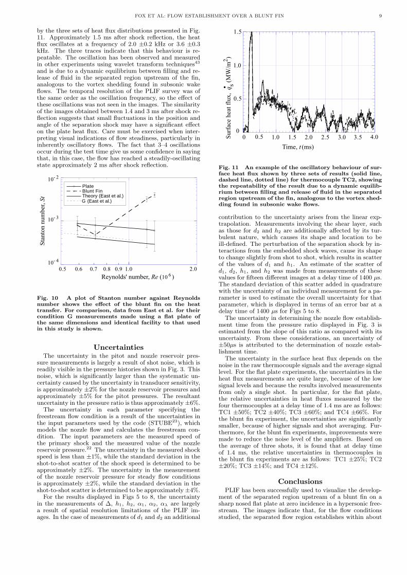
by the three sets of heat flux distributions presented in Fig.11. Approximately 1.5 ms after shock reflection, the heatflux oscillates at a frequency of 2.0 ±0.2 kHz or 3.6 ±0.3kHz. The three traces indicate that this behaviour is re-peatable. The oscillation has been observed and measuredin other experiments using wavelet transform techniques43and is due to a dynamic equilibrium between filling and re-lease of fluid in the separated region upstream of the fin,analogous to the vortex shedding found in subsonic wakeflows. The temporal resolution of the PLIF survey was ofthe same order as the oscillation frequency, so the effect ofthese oscillations was not seen in the images. The similarityof the images obtained between 1.4 and 3 ms after shock re-flection suggests that small fluctuations in the position andangle of the separation shock may have a significant effecton the plate heat flux. Care must be exercised when inter-preting visual indications of flow steadiness, particularly ininherently oscillatory flows. The fact that 3–4 oscillationsoccur during the test time give us some confidence in sayingthat, in this case, the flow has reached a steadily-oscillatingstate approximately 2 ms after shock reflection.

PlateBlunt FinTheory (East et al.)G (East et al.)

Fig. 10 A plot of Stanton number against Reynoldsnumber shows the effect of the blunt fin on the heattransfer. For comparison, data from East et al. for theircondition G measurements made using a flat plate ofthe same dimensions and identical facility to that usedin this study is shown.

UncertaintiesThe uncertainty in the pitot and nozzle reservoir pres-

sure measurements is largely a result of shot noise, which isreadily visible in the pressure histories shown in Fig. 3. Thisnoise, which is significantly larger than the systematic un-certainty caused by the uncertainty in transducer sensitivity,is approximately ±2% for the nozzle reservoir pressures andapproximately ±5% for the pitot pressures. The resultantuncertainty in the pressure ratio is thus approximately ±6%.

The uncertainty in each parameter specifying thefreestream flow condition is a result of the uncertainties inthe input parameters used by the code (STUBE23), whichmodels the nozzle flow and calculates the freestream con-dition. The input parameters are the measured speed ofthe primary shock and the measured value of the nozzlereservoir pressure.22 The uncertainty in the measured shockspeed is less than ±1%, while the standard deviation in theshot-to-shot scatter of the shock speed is determined to beapproximately ±2%. The uncertainty in the measurementof the nozzle reservoir pressure for steady flow conditionsis approximately ±2%, while the standard deviation in theshot-to-shot scatter is determined to be approximately±4%.

For the results displayed in Figs 5 to 8, the uncertaintyin the measurements of ∆, h1, h2, α1, α2, αλ are largelya result of spatial resolution limitations of the PLIF im-ages. In the case of measurements of d1 and d2 an additional

Fig. 11 An example of the oscillatory behaviour of sur-face heat flux shown by three sets of results (solid line,dashed line, dotted line) for thermocouple TC2, showingthe repeatability of the result due to a dynamic equilib-rium between filling and release of fluid in the separatedregion upstream of the fin, analogous to the vortex shed-ding found in subsonic wake flows.

contribution to the uncertainty arises from the linear exp-trapolation. Measurements involving the shear layer, suchas those for d2 and h2 are additionally affected by its tur-bulent nature, which causes its shape and location to beill-defined. The perturbation of the separation shock by in-teractions from the embedded shock waves, cause its shapeto change slightly from shot to shot, which results in scatterof the values of d1 and h1. An estimate of the scatter ofd1, d2, h1, and h2 was made from measurements of thesevalues for fifteen different images at a delay time of 1400 µs.The standard deviation of this scatter added in quadraturewith the uncertainty of an individual measurement for a pa-rameter is used to estimate the overall uncertainty for thatparameter, which is displayed in terms of an error bar at adelay time of 1400 µs for Figs 5 to 8.

The uncertainty in determining the nozzle flow establish-ment time from the pressure ratio displayed in Fig. 3 isestimated from the slope of this ratio as compared with itsuncertainty. From these considerations, an uncertainty of±50µs is attributed to the determination of nozzle estab-lishment time.

The uncertainty in the surface heat flux depends on thenoise in the raw thermocouple signals and the average signallevel. For the flat plate experiments, the uncertainties in theheat flux measurements are quite large, because of the lowsignal levels and because the results involved measurementsfrom only a single shot. In particular, for the flat plate,the relative uncertainties in heat fluxes measured by thefour thermocouples at a delay time of 1.4 ms are as follows:TC1 ±50%; TC2 ±40%; TC3 ±60%; and TC4 ±66%. Forthe blunt fin experiment, the uncertainties are significantlysmaller, because of higher signals and shot averaging. Fur-thermore, for the blunt fin experiments, improvements weremade to reduce the noise level of the amplifiers. Based onthe average of three shots, it is found that at delay timeof 1.4 ms, the relative uncertainties in thermocouples inthe blunt fin experiments are as follows: TC1 ±25%; TC2±20%; TC3 ±14%; and TC4 ±12%.

ConclusionsPLIF has been successfully used to visualize the develop-

ment of the separated region upstream of a blunt fin on asharp nosed flat plate at zero incidence in a hypersonic free-stream. The images indicate that, for the flow conditionsstudied, the separated flow region establishes within about

10 FOX ET AL: FLOW ESTABLISHMENT OVER A BLUNT FIN

1.5 ms, and that nominally steady flow conditions persistfor at least an additional 1.5 ms. Heat flux results indicatea similar starting time, but also exhibit oscillatory behaviorwhich continues throughout the test time. The test timeis sufficiently long-lived to allow 3-4 oscillations to occur.These results indicate that this type of quasi-steady viscousinteraction problem can be studied successfully despite thelimited test times of the free-piston shock tunnel.

The measured distance from the fin to the separationpoint is consistent with a transitional flow, situated betweenpreviously-measured values for flows having turbulent andlaminar approaching boundary layers. The heat flux dis-tribution during the test time shows undisturbed upstreamflow, a reduction in heat flux close to the separation pointand heat flux of 4-5 times the flat plate value downstreamof separation.

AcknowledgmentsThis study was carried out as part of a research program

supported by a Faculty Research Grant funded through theAustralian National University. The valuable discussionsof this work before and during experiments with CharlesHill and Matthew Gaston are gratefully acknowledged. Theauthors wish to thank Paul Walsh for the contribution ofhis technical expertise in this project.

References1Korkegi, R. H., “Survey of viscous interactions associated with

high Mach number flight,” AIAA Journal, Vol. 9, No. 5, May 1971,pp. 771–783.

2Stollery, J. L., “Some aspects of shock-wave boundary-layer in-teraction at hypersonic speed,” Proceedings of the 17th InternationalSymposium on Shock Waves and Shock Tunnels, Bethlehem, PA,American Institute of Physics, July 1989, pp. 12–22.

3Neumann, R. D. and Hayes, J. R., “Protuberance heating at highMach numbers - a critical review and extension of the data base,”AIAA Paper 81–0420, AIAA, Jan. 1981, St Louis, MO.

4McMaster, D. L. and Shang, J. S., “A numerical study of three-dimensional separated flows around a sweptback blunt fin,” AIAAPaper 88-0125, AIAA, Jan. 1988, In 26th Aerospace Sciences Meetingand Exhibit, Reno, NV.

5Stollery, J. L., “Some aspects of shock-wave boundary-layer in-teraction relevant to intake flows,” Paper 17, AGARD, Nov. 1987,AGARD Conference Proceedings, No. 428, Aerodynamics of hyper-sonic lifting vehicles.

6Kussoy, M. I. and Horstman, K. C., “Three-dimensional hyper-sonic shock wave / turbulent boundary-layer interactions,” AIAAJournal, Vol. 31, No. 1, Jan. 1993, pp. 8–9.

7Knight, D. D., Horstman, C. C., Shapey, B., and Bogdonoff,S., “Structure of supersonic turbulent flow past a sharp fin,” AIAAJournal, Vol. 25, No. 10, Oct. 1987, pp. 1331–1337.

8Settles, G. and Teng, H. Y., “Flow visualisation of separated 3-Dshock wave / turbulent boundary layer interactions,” AIAA Journal,Vol. 21, No. 3, March 1983, pp. 390–397.

9Roberts, G. T. and East, R. A., “Liquid crystal thermographyfor heat transfer measurement in hypersonic flows: a review,” J.Spacecraft and Rockets, Vol. 33, No. 6, Nov–Dec 1996, pp. 761–768.

10Roberts, G. T., Schuricht, P. H., and Mudford, N. R., “Heatingenhancement caused by a transverse control jet in hypersonic flow,”Shock Waves Journal, Vol. 8, No. 2, 1998, pp. 105–112.

11Watson, R. D. and Weinstein, L. M., “A study of hypersoniccorner flow interaction,” AIAA Journal, Vol. 9, No. 7, July 1971.

12Garrison, T. J., Settles, G. S., Narayanswami, N., and Knight,D. D., “Structure of crossing shock-wave / turbulent-boundary-layerinteractions,” AIAA Journal, Vol. 31, No. 12, Dec. 1993, pp. 2204–2211.

13Settles, G. S. and Dobson, L., “Supersonic and hypersonicshock/boundary layer interaction database,” AIAA Journal, Vol. 32,No. 7, July 1994, pp. 1377–1383.

14Olejniczak, J. and Candler, G. V., “Computation of hypersonicshock-interaction flow fields,” AIAA Paper 98–2446, AIAA, June1998, In 20th AIAA Advanced Measurement and Ground TestingTechnology Conference, Albuquerque, New Mexico, USA.

15Amaratunga, S. R., Tutty, O. R., and Roberts, G. T., “Compu-tations of laminar, high enthalpy air flow over a compression ramp,”SP 426, ESA, 1999, In 3rd European Symposium on Aerothermody-namics for Space Vehicles, ESA.

16Olejniczak, J., Candler, G. V., Wright, M. J., Hornung, H. G.,and Leyva, I. A., “High-enthalpy double-wedge experiments,” AIAAPaper 96–2238, AIAA, 1996, In AIAA Conference.

17Stalker, R. J., “Development of a hypervelocity wind tunnel,”Aeronautical Journal, Vol. 76, No. 738, June 1972, pp. 374–384.

18O’Byrne, S. B., Houwing, A. F. P., and Danehy, P. M., “Estab-lishment of the near-wake flow of a cone and wedge in a transienthypersonic freestream,” Proceedings of 22nd International Sympo-sium on Shock Waves, Imperial College, London, July 1999, pp.1583–1588.

19Mallinson, S. G., Gai, S. L., and Mudford, N. R., “The interac-tion of a shock wave with a laminar boundary layer at a compressioncorner in high-enthalpy flows including real-gas effects,” J. FluidMech., Vol. 342, No. 10, July 1997, pp. 1–35.

20Smith, C. E., “The starting process in a hypersonic nozzle,” J.Fluid Mech., Vol. 24, No. 4, 1966, pp. 625–640.

21Saito, T. and Takayama, K., “Numerical simulations of nozzlestarting process,” Shock Waves Journal, Vol. 9, No. 2, 1999, pp. 73–79.

22Boyce, R. R., Morton, J. W., Houwing, A. F. P., Mundt, C., andBone, D. J., “Computational fluid dynamics validation using multipleinterferometric views of a hypersonic flowfield,” Journal of Spacecraftand Rockets, Vol. 33, No. 3, 1996, pp. 319–325.

23Vardavas, I. M., “Modelling reactive gas flows within shock tun-nels,” Australian Journal of Physics, Vol. 37, No. 2, 1984, pp. 157–177.

24Davies, W. and Bernstein, J., “Heat Transfer and Transition toTurbulence in the Shock-Induced Boundary Layer on a Semi-InfiniteFlat Plate,” Journal of Fluid Mechanics, Vol. 36, No. 1, May 1969,pp. 87–112.

25Holden, M. S., “Establishment time of laminar separated flowswithin shock tunnels,” AIAA Journal, Vol. 9, No. 11, Nov. 1971,pp. 2296–2298.

26Eckert, E. R. G., “Engineering Relations for Friction and HeatTransfer to Surfaces in High Velocity Flow,” Journal of AeronauticalScience, Vol. 22, No. 8, Aug. 1955, pp. 585–587.

27Westkaemper, J. C., “Turbulent boundary layer separationahead of cylinders,” AIAA Journal, Vol. 6, No. 7, July 1968,pp. 1352–1355.

28Miles, J. W., Mirels, H., and Wang, H. E., “Time required forestablishing a detached bow shock,” AIAA Journal, Vol. 4, No. 6,June 1966, pp. 1127–1128.

29Hornung, H. G., “Non-equilibrium dissociating nitrogen flowover spheres and circular cylinders,” Journal of Fluid Mechanics,Vol. 53, No. 1, 1972, pp. 149–176.

30He, Y. and Morgan, R. G., “Transition of compressible high en-thalpy boundary layer flow over a flat plate,” Aeronautical Journal,Vol. 98, No. 2, 1994, pp. 25–33.

31Houwing, A. F. P., Palmer, J. L., Thurber, M. C., Wehe, S. D.,R. K, H., and Boyce, R. R., “Comparison of planar fluorescence mea-surements and computational modeling of a shock layer flow,” AIAAJournal, Vol. 34, No. 3, March 1996, pp. 470–477.

32Hiller, B. and Hanson, R. K., “Simultaneous planar measure-ments of velocity and pressure fields in gas flows using laser-inducedfluorescence,” Appl. Opt., Vol. 27, No. 1, Jan. 1988, pp. 33–48.

33Fox, J. S., Gaston, M. J., Houwing, A. F. P., Danehy, P. M.,Mudford, N. R., and Gai, S. L., “Instantaneous mole-fraction PLIFimaging of mixing layers behind hypermixing injectors,” AIAA paper99-0774, AIAA, 1999, In 37th AIAA Aerospace Sciences Meeting andExhibit, Reno, NV.

34McIntyre, T. J., Houwing, A. F. P., Palma, P. C., Rabbath, P.,and Fox, J. S., “Imaging of combustion in a supersonic combustionramjet,” Journal of Propulsion and Power , Vol. 13, No. 3, May 1997,pp. 388–394.

35Hill, C. D., Danehy, P. M., Fox, J. S., Houwing, A. F. P., andGaston, M. J., “Instantaneous temperature imaging in a free-pistonshock tunnel,” Proceedings of 2nd Australian Conference on LaserDiagnostics in Fluid Mechanics and Combustion, Melbourne, Aus-tralia, Dec. 1999, pp. 109–110.

36Palma, P. C., Houwing, A. F. P., and Sandeman, R. J., “Abso-lute intensity measurements of impurity emissions in a shock tunneland their consequences for laser induced fluorescence experiments,”Shock Waves Journal, Vol. 3, No. 1, 1993, pp. 49–53.

37Hung, C. M. and Buning, P., “Simulation of blunt-fin-inducedshock-wave and turbulent boundary layer interaction,” J. FluidMech., Vol. 154, May 1985, pp. 163–185.

38Dolling, D. S. and Bogdonoff, S. M., “Blunt fin-induced shockwave/turbulent boundary layer interaction,” AIAA Journal, Vol. 20,No. 12, Dec. 1978, pp. 1674–1680.

39Hung, F. T. and Clauss, J. M., “Three dimensional protuberanceinterference heating in high-speed flow,” AIAA Paper 80-0289, AIAA,1980, In AIAA Conference.

40Diller, T. E., “Advances in heat flux measurements,” Advancesin Heat Transfer , Vol. 23, 1993, pp. 279–368.

41Schuricht, P. H. and Roberts, G. T., “Hypersonic interferenceheating induced by a blunt fin,” AIAA Paper 98–1579, AIAA, 1998,In AIAA 8th International Space Planes and Hypersonic Systems andTechnologies Conference, Norfolk, Virginia.

42East, R. A., Stalker, R. J., and Baird, J. P., “Measurement ofheat transfer to a flat plate in a dissociated high-enthalpy laminar airflow,” J. Fluid Mech., Vol. 97, No. 4, 1980, pp. 673–699.

43Poggie, J. and Smits, A. J., “Wavelet analysis of wall-pressurefluctuations in a supersonic blunt-fin flow,” AIAA Journal, Vol. 35,No. 10, Oct. 1997, pp. 1597–1603.