Fluid Simulation for Video Games (part 3) - Intel® … · Fluid Simulation for Video Games (part 3) ... other fluid simulation techniques that ... how to discretize a continuum so

Fluid Simulation for Video Games (part 3) By Dr. Michael J. Gourlay

Vortex Particle Fluid Simulation

This article, the third in a series, presents a fluid simulation implemented in C++ that runs

in real time using modest and commonly available computer hardware. The first article

summarized fluid dynamics; the second surveyed fluid simulation techniques.

The simulation presented here uses vortex particles, called vortons by Novikov (1983), to

represent the flow field and solves for velocity at each time. This tactic of using vortons

preserves vorticity without obvious sources of diffusion, which allows the simulation to

retain fine-scaled details. In contrast, other fluid simulation techniques that use primitive

variables (velocity and pressure) or grids numerically diffuse vorticity, so the flow tends to

look thick and syrupy. When you see the results of this simulation, you will be surprised at

how much motion detail it preserves, considering how fast it runs.

This simulation also exploits the embarrassingly parallel nature of the algorithms and uses

Intel® Threading Building Blocks (TBB) to spread the work across multiple threads.

In the endeavor to achieve real-time fluid motion, some other fluid simulations exploit

general-purpose computing on graphics processing unit (GPGPU). However clever, such

approaches do not help with current gaming hardware, because in video games, the GPU

tends to be busy with rendering and has no time left over for simulation. So obtaining real-

time speeds using the GPU does not provide a viable solution for current video games. The

solution needs to run fast enough to execute in whatever time remains available on the

CPU.

Source code accompanies this article, which overviews the concepts behind the simulation,

but for the sake of brevity this article stops short of providing a line-by-line commentary of

2 Fluid Simulation for Video Games (part 3)

4 August 2009

the code. I did, however, strive to comment the code thoroughly, so please see the code for

further details.

The sections below describe the steps in implementing a fluid simulation: The first section

describes spatial partitioning and discretization, converting from an infinite continuum

into a finite discrete problem. The next section describes how to employ that discretization

to formulate the fluid dynamics equations into a form suitable for processing on a

computer. Finally, you get to see some results aimed at demonstrating the viability of this

simulation.

The next article explains two-way fluid-body interactions, and subsequent articles cover

performance analysis, optimization, further parallelization, and how to integrate this

simulation into a game engine.

Discretization

The second article introduced a taxonomy of simulation techniques that included grid-

based and mesh-free varieties. This simulation uses a mesh-free scheme for representing

vorticity and advecting (that is, moving) vortons and a grid-based scheme for interpolating

velocity between points, computing spatial derivatives, and searching for nearest

neighbors. That makes this simulation a hybrid: vortons (which carry vorticity) and other

particles (which facilitate visualization) can move anywhere, but this simulation ascribes

other fluid properties (like velocity) only at fixed locations on a uniform grid. In some ways,

this simulation resembles a vortex-in-cell simulation as described, for example, by Cottet

and Koumoutsakos (2000).

Mesh-free Vortex Particles (Vortons)

Using vortons to represent the flow field provides at least one major benefit over other

techniques, such as smoothed particle hydrodynamics (SPH) or Eulerian schemes: The

vortons have no obvious unintentional numerical diffusion of vorticity. The motion does

not artificially dampen, which allows the flow to have low viscosity and maintain fine-scale

details.

SPH and Eulerian schemes suffer dramatically from numerical viscosity, which arises either

explicitly (by cranking up viscosity) or implicitly (from the implicit solver), and is a

necessary evil that combats numerical instability. (See the discussion of stability in part 2.

Also note that those numerically dissipative schemes can use “vorticity confinement” to re-

inject motion at small scales, which sometimes yields interesting results. See Steinhoff and

Underhill (1994) for more information.)

As described in the part 2, vorticity could be discretized into points (particles, or vortons),

curves (filaments) or surfaces (sheets or panels). All have their merits, but this article has

Fluid Simulation for Video Games (part 3) 3

4 August 2009

room for only one, and particles are the simplest. But bear in mind that the other

discretizations also have benefits, including dodging numerical diffusion.

Using a Lagrangian (particle) approach also provides the benefit that vorticity can advect

outside the original domain, whereas with Eulerian (grid) approaches, allowing fluid to

flow out of a domain can be problematic. This means that you do not have to know in

advance where the fluid will flow; the vortons simply go where they need to, without any

complicated outflow (such as so-called continuative or radiation) boundary conditions or

temperamental regridding schemes.

In this simulation, the C++ class Vorton represents a vortex particle. Each vorton has a

position and a vorticity. (The Vorton class also has other members, explained below.)

Uniform Grid

Although this simulation uses vortex particles to carry information about the fluid flow and

those particles are free to move anywhere, the simulation also uses a uniform grid to

simplify and expedite certain calculations: calculating velocity from vorticity, interpolating

velocity values between grid point (or between vortons), and computing spatial

derivatives. (Details of those calculations appear in later sections.) This section describes

the uniform grid as a kind of container, not entirely unlike a Standard Template Library

container.

Most Eulerian simulations rely heavily on uniform grids for storing data and performing

computations on that data. Although the simulation presented in this article is primarily

Lagrangian, not Eulerian, some of the techniques that apply to Eulerian approaches could

also apply to this one. Future articles could explore some ways to hybridize these

approaches even further.

This simulation represents uniform grids as a C++ templated UniformGrid class, whose

template argument is, as is typical for container classes, the data type contained by the

class. The UniformGrid class inherits from a base class called UniformGridGeometry,

so let’s start there.

The UniformGridGeometry class (which is not a templated class—just a regular class)

contains information about the shape and size of the region that the uniform grid

represents. The constructor provides the means to decide the shape and size automatically

given corners of the axis-aligned bounding box and the number of items to be contained.

When creating a UniformGrid to contain particles, you first need to find the bounding

box that contains all particles, and you need to know the total number of particles. Both of

those are readily available, so you have what we need. The UniformGridGeometry

constructor and the DefineShape method use that information to create grid geometry

suitable to contain information about all the vortons.


4 August 2009

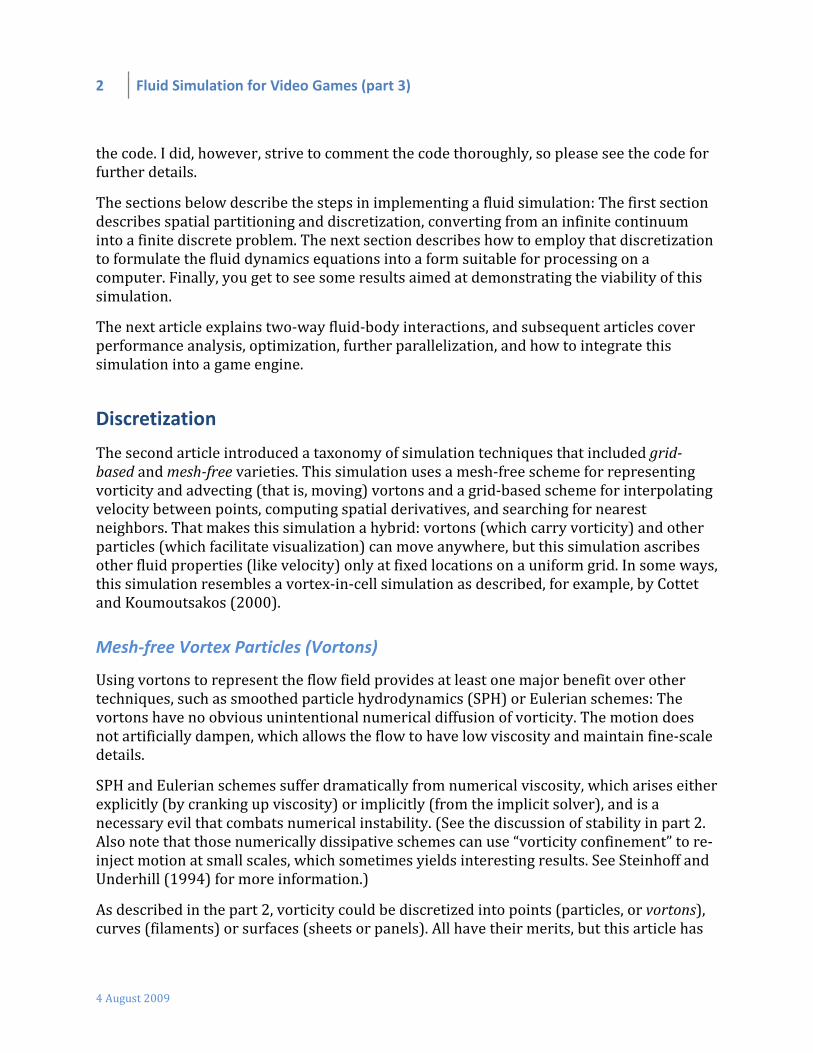
A uniform grid is a grid in which every cell has the same size as every other. This uniformity

makes spatial lookups computationally trivial, because, given a location ��, you can compute

the index {ix,iy,iz} of the cell that contains that location from

�� = (�� − ��)�

where �� is the minimum corner of the bounding box, � is the size of the bounding box, and

the subscript � indicates each of the directions x, y, or z. The routine

UniformGridGeometry::IndicesOfPosition computes these indices given a

position.

The UniformGrid extends UniformGridGeometry by associating data with each grid

point. Interpolating data values between grid points is straightforward. Given a position,

you can find the grid cell that contains it and therefore all grid points that surround that

grid cell. Figure 1 shows the relationship between grid points and grid cells. Knowing the

eight grid points (and their associated data) that surround a grid cell allows you to linearly

interpolate a data value anywhere inside the grid cell. (If you required higher accuracy, you

could use higher-order interpolation schemes such as tricubic or even spectral methods

that use data from the whole domain, not just adjacent grid points.) The method

UniformGrid::Interpolate performs this calculation.

Figure 1. Uniform grid spatial partition

Uniform grids also allow straightforward computation of spatial derivatives using either

finite differences or spectral methods. The simulation that accompanies this article uses a

Grid cell

…this

grid cell.

Grid

point

Minimal

grid point

This grid point…

Maximal

grid point

…“owns”…


4 August 2009

centered-difference scheme, as described in the second article, expressed as � �� ≈ (��)� (��)

�� .

It turns out that for this simulation, you need to compute all partial derivatives of all

components (x, y, and z) of velocity ��≡⟨�, �, �⟩. In other words, you need each of the

following:

�� !�� !�� ! "#

####$≡%(��)

This is called the Jacobian matrix, and the routine ComputeJacobian computes it for any

UniformGrid that contains a 3-vector quantity, such as velocity.

To compute velocity from vorticity, the simulation effectively integrates vorticity

everywhere in space (described in further detail below), but performing that computation

in the obvious way would cost too much time. So instead, you use an approximation that

relies on structuring data hierarchically. So, in addition to facilitating interpolation and

computation of spatial derivatives, UniformGrid serves as the basis for a set of nested

grids that represents this hierarchy.

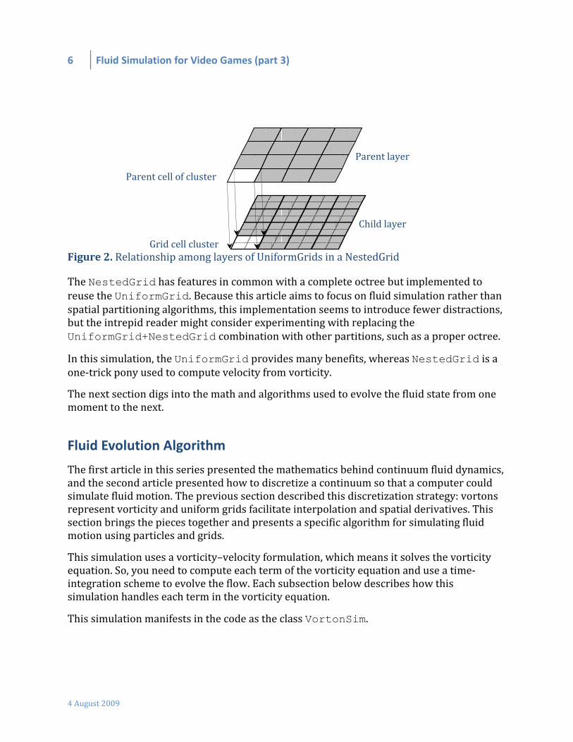
Nested Grid

The NestedGrid class is another C++ templated container class that builds upon the

UniformGrid container. This vorton simulation uses NestedGrid to aggregate vorticity

information to compute velocity from vorticity (as described further below). The concept is

straightforward but easier to explain with pictures than words, so look at Figure 2. Think of

a NestedGrid as a series of layers of UniformGrids, all with the same bounding box. At

the finest scale of the NestedGrid is the base layer, which is the UniformGrid that has

the largest number of cells and the highest resolution. Above that is another

UniformGrid that has fewer cells, which I will call the parent layer. Each cell in the parent

layer represents a cluster of constituent cells in the child layer. Likewise, the parent has

another layer above it (and I’ll resist the temptation to call it a grandparent, but you get the

idea), whose cells represent clusters of cells in this parent. Et cetera. The top layer in this

tree has a single cell, the root.


4 August 2009

Figure 2. Relationship among layers of UniformGrids in a NestedGrid

The NestedGrid has features in common with a complete octree but implemented to

reuse the UniformGrid. Because this article aims to focus on fluid simulation rather than

spatial partitioning algorithms, this implementation seems to introduce fewer distractions,

but the intrepid reader might consider experimenting with replacing the

UniformGrid+NestedGrid combination with other partitions, such as a proper octree.

In this simulation, the UniformGrid provides many benefits, whereas NestedGrid is a

one-trick pony used to compute velocity from vorticity.

The next section digs into the math and algorithms used to evolve the fluid state from one

moment to the next.

Fluid Evolution Algorithm

The first article in this series presented the mathematics behind continuum fluid dynamics,

and the second article presented how to discretize a continuum so that a computer could

simulate fluid motion. The previous section described this discretization strategy: vortons

represent vorticity and uniform grids facilitate interpolation and spatial derivatives. This

section brings the pieces together and presents a specific algorithm for simulating fluid

motion using particles and grids.

This simulation uses a vorticity–velocity formulation, which means it solves the vorticity

equation. So, you need to compute each term of the vorticity equation and use a time-

integration scheme to evolve the flow. Each subsection below describes how this

simulation handles each term in the vorticity equation.

This simulation manifests in the code as the class VortonSim.

Parent layer

Child layer

Grid cell cluster

Parent cell of cluster


4 August 2009

Velocity from Vorticity

Several terms in the vorticity equation require velocity. Recall from the first article that you

can compute flow velocity �� at position �� that is a distance &� = �� − ��′ from a volume

element (��′ with vorticity )�� by integrating over all space:

��(��) = 14, - )��(��′) × &�&/ (��′ If you represented vorticity only at N infinitesimal points (that is, the locations of the

vortons), the integral becomes a simple summation:

��(��) = 14, 0 )1�� × &1��&2/3

245

where the subscript i indicates the vorton index. The

VortonSim::ComputeVelocityBruteForce method implements this direct

summation algorithm. Computing this at every vorton requires O(N2) operations, which

would become excessively expensive for more than a very small number of vortons.

This formula has a problem: When the distance from a vorton ri is very small, the

contribution due to that vorton becomes very large, and as ri approaches zero, the

contribution approaches infinity. This is called a singularity, and it causes numerical

problems. To avoid those problems, give each vortex a tiny size, 6. Outside of that region,

vorticity is zero, and the velocity field acts as though it came from a point vorton,

resembling the simple formula above. Inside that region, however, vorticity drops so that

the velocity approaches zero linearly as the radius approaches zero:

�� = 14, 0 )1�� × &1��3

24572 8&2�/: & ≥ 662�/: & ≤ 6<

Here, 72 is the volume of the vortex element, which is a tiny blob instead of a zero-sized

point, but you still call it a vorton. This model resembles that of a so-called Rankine vortex.

The resulting vorticity is said to be mollified, and avoiding the singularity in this way is

called regularization. The Vorton::AccumulateVelocity method implements the

formula inside the summation. Problem solved.

To reduce the computational complexity of this direct summation, take advantage of the

fact that when “felt” from far away, the influence of a cluster of vortons “feels”

approximately the same as a single “supervorton” whose circulation is the same as the sum

of circulation of all the vortons in the cluster. Figure 3 offers a picture of this phenomenon.


4 August 2009

Figure 3. Clusters of distant vortons “feel” almost the same as a single supervorton.

You put this idea into practice by creating clusters of vortons, then creating clusters-of-

clusters, and so on, until the entire field of vortons is represented by a single cluster, as

depicted in Figure 4. I refer to this tree of vorton clusters as the influence tree, and this is

where the NestedGrid comes into play.

Figure 4. Vorton cluster influence tree. Each ancestor node represents its constituents as a

single supervorton.

The influence tree is a NestedGrid of vortons, and the VortonSim class contains a

member named mInfluenceTree that is exactly this. The method

CreateInfluenceTree constructs the influence tree in two phases: building the base

layer and aggregating clusters.

Each layer in the tree is a UniformGrid of information. Each grid cell contains a vorticity

and a position, stored as a representative “supervorton.” The vorticity of a supervorton is

the aggregate vorticity of all constituent vortons in that cell, and its position ��= is the

“center of vorticity,” which is the average position of all constituent vortons in the cluster,

where each vorton position ��2 is weighted by )2 , the magnitude of its vorticity:

��= = 0 )2��23

245 .

So, stronger constituent vortons have more influence over the position of the supervorton

that represents them.

Vortons

Supervortons

Vortices

approach

each other

Query about

their influence at

some distance

Query point is

far compared

to vortex

separation

Vortices

separated by a

small distance

? ?


4 August 2009

The method MakeBaseVortonGrid creates the base layer. It copies information from the

array of vortons into a UniformGrid, obeying the rules that apply to aggregation. This

routine effectively takes an array of vortons and turns them into a uniform grid of

supervortons.

The method AggregateClusters aggregates vorticity information of clusters of cells in

the child layer into cells in the parent layer that represent those clusters as a single

supervorton.

Note Astute readers might notice that each layer in the influence tree includes information that is not used, such

as the velocity of each cluster. It seems as though we should separate the vorton into two classes: one with

velocity and another without. The apparently extraneous velocity member will come in handy, however, in an

aggressive optimization that will appear in a future article.

The influence tree represents vortons and clusters of vortons, where each cell contains at

most one supervorton. You use that tree to compute velocity from vorticity. That process

entails a straightforward recursive tree traversal, making this algorithm a so-called tree

code, as described by Barnes and Hut (1986), although they formulated their algorithm for

gravitational problems like galaxy formation, and they constructed their tree in subtly

different ways.

To compute velocity at a given point, traverse the influence tree as follows (and as shown

in Figure 5): Start at the root of the influence tree. For each octant in the tree, if the octant

does not contain the query point (or if this is a leaf node), then compute the contribution to

velocity due to the sole supervorton in that octant as though it were an ordinary vorton.

Otherwise, if the octant does contain the query point, descend the tree at that octant. That’s

it!


4 August 2009

Figure 5. Influence tree traversal for obtaining velocity at query point Q

As a refinement, let us reconsider the descent criterion. The simplest is the one described

above: Only descent into octants that contain the query point. You can improve accuracy by

augmenting that criterion to be “descend into octants that are within a threshold distance

of the query point.” Then, you can tune that “threshold distance” to obtain the desired

accuracy. If you made the threshold distance very large, then the algorithm effectively

devolves into the O(N2) brute-force direct summation algorithm. For visual effects,

however, you can turn that threshold down to zero and obtain acceptable results.

Another detail remains—and this is where you depart from a purely Lagrangian treatment.

It would seem natural to evaluate velocity at each vorton and advect the vortons

accordingly. In fact, this is a traditional approach, and it works just fine. But this simulation

does something different.

The VortonSim::ComputeVelocityGrid method evaluates velocity at each point on a

grid, and then routines that need velocity interpolate values from the grid. At first glance,

this interpolation step might seem extraneous, not to mention that by interpolating you

reduce the precision of the velocity calculation. But having velocity on a grid turns out to

provide benefits that outweigh this drawback.

Interpolation on a uniform grid is much faster than computing velocity using the tree—

perhaps 10 times faster or more. The UniformGrid::Interpolate method performs

Start

here

root This octant does NOT contain query point Q.

Apply influence of whole cluster.

This octant DOES contain query point Q.

Recursively descend.

Q


4 August 2009

this computation. Because several routines need to compute velocity at specific locations,

using the grid as an intermediary speeds up access to velocity compared to computing it

using the influence tree.

Also, creating a velocity grid allows you to vary the resolution of the velocity grid

independently of the number of vortons. So if you wanted to, you could intentionally

reduce the resolution of the velocity grid to gain more speed at the cost of accuracy. Or vice

versa.

Finally, computing velocity on a grid simplifies the calculation of spatial derivatives, which

you need to compute other terms in the vorticity equation, such as vortex stretching and

tilting.

Vortex Stretching and Tilting

The stretching and tilting term of the vorticity equation (described in the first two articles

and expressed as @)�� ∙ B��C��) involves spatial derivatives—specifically, the gradients of

velocity. You can expand that term to obtain

)� DE��D� + )G DE��

DG + )H DE��DH =

��DE

D�DEDG

DEDHDI

D�DIDG

DIDHDJ

D�DJDG

DJDH "#

##$

K)�)G)HL = %(��))�� .

In other words, you transform the vorticity of every vorton by the Jacobian matrix of

velocity. You compute the Jacobian at every point on the velocity grid (using

ComputeJacobian), then interpolate the Jacobian at each vorton. Fortunately, because

you wrote UniformGrid as a template, the Interpolate method works identically for

both vectors and matrices, so you do not need to write additional code. You simply need to

evaluate the stretching and tilting formula at each vorton, and then update the vorticity of

each vorton accordingly using some time integration scheme such as the explicit Euler

method. The VortonSim::StretchAndTiltVortons method accomplishes this.

Note The stretching and tilting term can accumulate errors in vorticity in the form of an irrotational component;

vorticity can accumulate divergence. Mathematically, it is impossible for the curl of a field to have divergence.

Because vorticity is the curl of velocity, vorticity should not have divergence. But numerically, divergence occurs as

a result of round-off and truncation errors. This divergence turns out not to have an immediate impact on the

velocity, but it does affect the stretching and tilting term, so it would be nice to eliminate it. There are clever ways

to do this by modifying the stretching and tilting computation, and a future article will revisit this topic. For now,

suffice it to say that because the goal is to make eye candy, as long as the simulation does not explode, you can

squeak by with this inaccuracy—at least for one or two articles.


4 August 2009

Diffusion: Particle Strength Exchange

Viscous vortex diffusion effectively smears vorticity. Mathematically, it has the form MBN)��,

where M is viscosity and BN = DOD�O + DO

DGO + DODHO is the Laplacian operator, which is a second

spatial derivative. Computing this with finite differences would be problematic, but

fortunately there is another way. Effectively, this operator behaves like a blurring operator:

It spreads vorticity across space. So, you can implement this as an exchange of vorticity

between vortons.

The mathematical derivation, omitted for brevity, entails replacing the differential operator

with an integral one. Here, you drastically simplify the approach, boiling it down to its

qualitative essentials: Vortons exchange a fraction of their vorticity with other vortons in

their vicinity.

This process requires knowing the nearest neighbors for each vorton. A common solution

to that problem entails using a spatial partition such as an octree or kD tree and performing

a nearest-neighbor search, but that solution costs O(log N) time per search. In contrast, this

simulation simplifies and accelerates this search by reusing UniformGrid, where the

contained data at each grid point is an array of indices into the array of vortons—that is,

vector<int>. So, each grid cell can contain references to multiple vortons. After

populating the search grid with vorton references, each vorton finds its nearest neighbors

as depicted in Figure 6.

Figure 6. Nearest neighbors of a vorton

In a fluid with viscosity parameter M, each vorton p then exchanges a portion of its vorticity )��Pwith its N neighbors, indexed by i, using the formula

When looking for nearest neighbors, each

vorton only seeks other vortons either in its

own cell, or in adjacent cells “in front of” its

own cell.

This works out, because vortons “behind” it

seek it, and after a vorton finds its neighbors,

they talk to each other both ways.


4 August 2009

()��P(Q = M 0()��2 − )��P3

245)

The method VortonSim::DiffuseVorticityPSE implements this formula by

considering pairs of vortons, in which case you can rewrite the formula as �R��S = M()��N − )��5) �R��O�S = M()��5 − )��N) = − �R��S .

This form shows that this exchange preserves total circulation (assuming that the particles

have the same size, which, in this simulation, they do).

Note To the extent that you care about physical accuracy, note that this formulation oversimplifies the situation.

For example, it neglects the distance between vortons and also their size, which is related to the spacing between

them. Among other things, that effectively means that the parameter M is not exactly the same as kinematic

viscosity. Readers curious to know more should read a detailed treatment, including a derivation of this approach,

in Degond and Mas-Gallic (1989).

Advection

The vorticity equation includes an advective acceleration term, which the first article

describes in detail as the nonlinear term that accounts for the characteristic motion that

makes a fluid look like a fluid. In the Lagrangian form of the vorticity equation, this term

basically means that vortons follow the flow—that is, they move according to the velocity

of the fluid, local to their current location. So, you need to know the velocity at the location

of each vorton, and the velocity grid gives you that.

Using the velocity grid, the VortonSim::AdvectVortons method interpolates to obtain

velocity at each vorton and moves the vorton accordingly (for example, using explicit

Euler). Fast interpolation using the velocity uniform grid allows you to advect other

particles—call them passive tracers—with ease. Indeed, VortonSim::AdvectTracers

does just that. You can then populate the simulation with many of these passive tracers and

render them or use them for other purposes, such as approximating aerodynamic drag by

colliding them with rigid bodies, which the next article covers.

Parallelization

Many of the routines in this simulation are embarrassingly parallel, meaning that the

operations and data of the calculations are independent of each other. This begs for data

parallelism. This simulation code uses Intel® TBB to parallelize certain routines. The TBB

construct parallel-for is well suited to the kind of data parallelism that pervades this

simulation.


4 August 2009

The routines that have a good combination of independence and slow run times include

CreateVelocityGrid and FillVertexBuffer. Each of these therefore uses TBB’s

parallel_for to run across multiple threads. Each of those routines has an associated

helper routine that operates on a subset (which the code calls a slice) of the total data, and

then uses a function object, which is an object that overrides operator(), to inform TBB

how to execute the process.

In the case of CreateVelocityGrid, each slice includes a subset of the Z values in the

volume of the velocity grid. Because assigning each grid point of the velocity requires no

information from any other part of the velocity grid, no synchronization is required.

In the case of FillVertexBuffer, each slice includes a subset of the particles. Because this

simulation uses a large number of passive tracer particles, this turns out to be a natural fit

for data parallelism.

Ironically, the slowest portion of this simulation is rendering the particles, which takes

more than half the time. You could speed up this time using programmable shaders, point

sprites or vertex buffer objects, but rendering topics lie outside the scope of this article.

Results

It is customary to demonstrate the validity of a simulation algorithm by applying it to

various well-known problems and comparing the results to expected solutions. For the

sake of brevity and following the tradition established in the computer graphics and

animation community, this article forgoes rigorous analysis and instead relies on visual

inspection to validate the results.

You might think that because this simulation uses vorticity, you should specify the initial

conditions directly in the form of a vorticity field. Not so. The preferred way to establish

initial conditions for any simulation that uses a vorticity–velocity formulation is to

formulate the velocity field you want, then take the curl of that field and initialize vorticity

that way. The routines ComputeCurlFromJacobian and

VortonSim::AssignVortonsFromVorticity facilitate this approach. This extra step

prevents the initial vorticity field from having an irrotational component (that is, from

having divergence). Be aware, however, that some of the test cases presented here were

created by specifying vorticity directly, and the initial vorticity does have divergence. This

is intentional, because although I claim that you want to exclude divergence from the initial

conditions, the simulation ought to be able to handle its presence.

Let’s look at some scenarios:

• A vortex ring, which self-propagates


4 August 2009

• A pair of crossed vortex tubes, which causes drastic stretching, allowing you to see

stretching occur in the expected place and direction

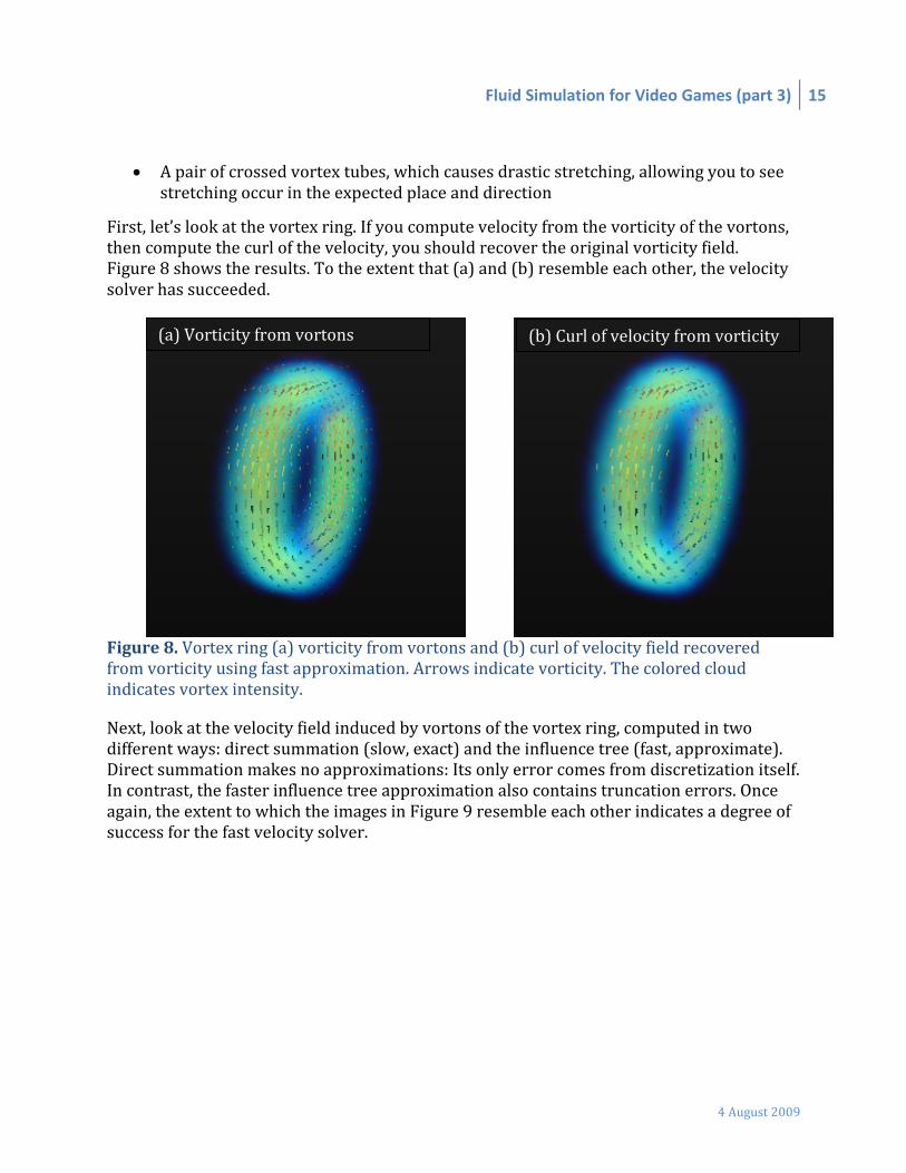
First, let’s look at the vortex ring. If you compute velocity from the vorticity of the vortons,

then compute the curl of the velocity, you should recover the original vorticity field.

Figure 8 shows the results. To the extent that (a) and (b) resemble each other, the velocity

solver has succeeded.

Figure 8. Vortex ring (a) vorticity from vortons and (b) curl of velocity field recovered

from vorticity using fast approximation. Arrows indicate vorticity. The colored cloud

indicates vortex intensity.

Next, look at the velocity field induced by vortons of the vortex ring, computed in two

different ways: direct summation (slow, exact) and the influence tree (fast, approximate).

Direct summation makes no approximations: Its only error comes from discretization itself.

In contrast, the faster influence tree approximation also contains truncation errors. Once

again, the extent to which the images in Figure 9 resemble each other indicates a degree of

success for the fast velocity solver.

(b) Curl of velocity from vorticity (a) Vorticity from vortons


4 August 2009

Figure 9. Velocity field recovered from vorticity of vortex ring using (a) direct summation

and (b) the influence tree approximation. Arrows indicate velocity flow field. The

orange/red cloud indicates velocity moving along +X, and the blue/green cloud indicates

velocity moving along –X. Lines indicate streamlines—that is, paths particles would take as

they follow the flow.

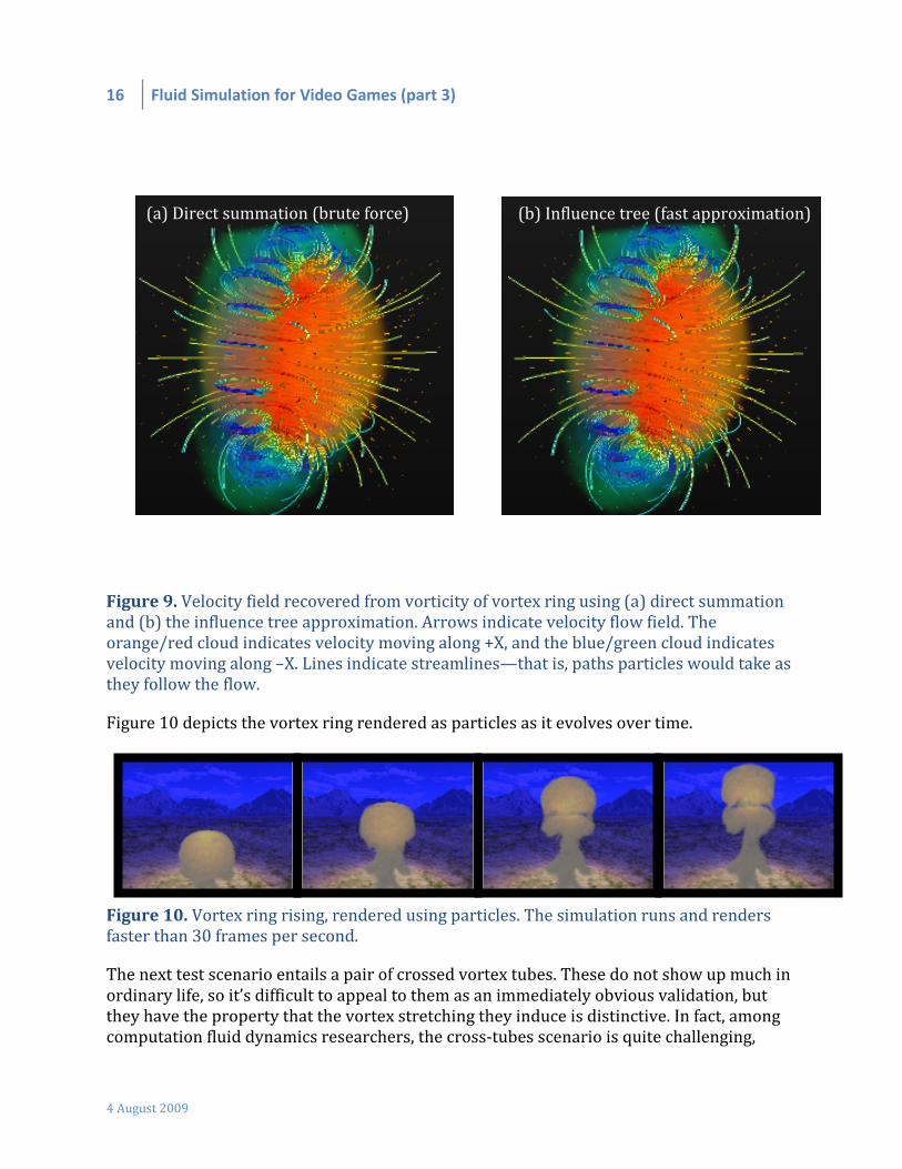
Figure 10 depicts the vortex ring rendered as particles as it evolves over time.

Figure 10. Vortex ring rising, rendered using particles. The simulation runs and renders

faster than 30 frames per second.

The next test scenario entails a pair of crossed vortex tubes. These do not show up much in

ordinary life, so it’s difficult to appeal to them as an immediately obvious validation, but

they have the property that the vortex stretching they induce is distinctive. In fact, among

computation fluid dynamics researchers, the cross-tubes scenario is quite challenging,

(b) Influence tree (fast approximation) (a) Direct summation (brute force)


4 August 2009

because it can result in creating a vortex of infinite strength, in finite time. It’s heady stuff,

and this article glosses over it, but to the scrutinizing observer, the images in Figure 11

indicate that stretching does indeed occur in the expected configuration.

Figure 11. Crossed vortex tubes (a) vorticity, (b) velocity, and (c) vortex stretching and

tilting

Although these results do not prove that this simulation is correct, they demonstrate that

the code produces plausible and appealing results at interactive speeds, and for visual

effects in video games, that can suffice. I encourage you to take a closer look at the routines

in the simulation code that compute and track quantities that should be conserved, such as

total circulation, hydrodynamic impulse, and angular impulse, and experiment with them.

It would be natural at this stage to report performance and compare that with other

techniques, and indeed future articles in this series will focus on performance analysis and

comparisons. For now, I simply report that these simulations run and render faster than 30

frames per second on a modest laptop using a single 2.5 GHz core of an Intel® Core™2 Duo

processor and faster than 60 frames per second—with only 35% CPU utilization—on a

machine with dual 2.33 GHz Quad-Core Intel® Xeon® processors. Most of that time is

spent waiting on the GPU to finish rendering, which has nothing to do with the algorithms

presented in this article. So, this simulation runs fast. And by the end of this series of

articles, it will run even faster.

Summary

This article presents a vortex particle treecode that uses a nested grid to compute velocity

from vorticity and uses uniform grids to compute spatial derivatives for stretching and

(a) Vorticity (b) Velocity (c) Stretching and tilting


4 August 2009

tilting. The uniform grid also expedites finding nearest neighbors to compute viscous

diffusion of vorticity using a particle strength exchange scheme. The simulation transports

vortex particles to account for advective acceleration, the nonlinear term that accounts for

the motion that makes a fluid move like a fluid. Finally, this simulation exploits the

embarrassingly data-parallel nature of the algorithms and uses Intel® TBB parallel-for

construct to spread the computational cost across multiple threads.

The resulting simulation runs and renders all of its demonstration cases faster than 30

frames per second on a modest laptop and faster than 60 frames per second on a multi-

core desktop computer.

This simulation code resembles a hybrid between a traditional tree code and a vortex-in-

cell scheme. You could modify this code to bridge that gap by using an off-the-shelf Poisson

solver to obtain velocity from vorticity. You can also explore using different stretching and

tilting formulae to mitigate problems that arise because of a spurious divergence in the

vorticity field.

The next article explains how to satisfy boundary conditions and support two-way fluid-

body interaction, and subsequent articles cover performance analysis, optimization and

integration into a game engine.

Further Reading

Novikov, E.A. 1983. Generalized dynamics of three-dimensional vortex singularities (vortons). Zhurnal

Eksperimental'noi i Teoreticheskoi Fiziki 84:975–81.

Beale, J.T. 1986. A convergent three-dimensional vortex method with grid-free stretching, Math Comp

46:401–24.

Degond, P., and S. Mas-Gallic. 1989. The weighted particle method for convection-diffusion equations, part 1:

the case of an isotropic viscosity. Math Comput 53(188):485–507.

Steinhoff, J., and D. Underhill. 1994. Modification of the Euler equations for “vorticity confinement”:

application to the computation of interacting vortex rings. Physics of Fluids 6(8):2738–44.

Cottet, GH., and P.D. Koumoutsakos. 2000. Vortex Methods: Theory and Practice. Cambridge: Cambridge UP.

Li, S., and W.K. Liu. 2004. Meshfree Particle Methods. New York: Springer-Verlag.

Bridson, R. 2008. Fluid Simulation for Computer Graphics. Wellesley, Mass.: A.K. Peters.

Froemke, Q. 2009. Multi-threaded fluid simulation for games. Gamasutra, June 17.

Documents

Fluid Simulation for Video Games (part 3) - Intel® … · Fluid Simulation for Video Games (part 3) ... other fluid simulation techniques that ... how to discretize a continuum so