Date : ____________

EXPERIMENT NO :

Name of the Experiment : To verify ‘ Bernoulli’s Theorem ’.

Apparatus : Bernoulli’s apparatus, Controlling valve at inlet and outlet,

Discharge Measuring Tank, Scale, Stopwatch etc.

Formula : P / W + V22 + 2 = constant

Where, P / W = Pressure energy V2 / 2g = Kinetic energy Z = Potential energy

Theory : The Bernoulli’s theorem states that the total energy / N of

flowing, non Viscous in compressible fluid in a steady state of flow, remains constant along a stream line Daniel Bernoulli’s enunciated in 1738 that is “ In any stream flowing steadily without friction, the total energy contained in a given mass is some at energy contained in a given mass is some at energy point in its path of flow.” This statement is called Bernoulli’s theorem with reference to section 1 – 1 and 2 – 2 along the length of steady flow in the stream tube shown in fig. The total energy at section 1 – 1 is equal to the total energy - at section 2 – 2 as stated in Bernoulli’s theorem. With usual notations, the expression for total energy contained in a unit wt of fluid at section 1 – 1 and 2 – 2 is given by

Total energy at Section 1 – 1 = P1 / W + V12 / 2g +Z1

Total energy at section 2 – 2 = P2 / W + V22 / 2g +Z2

Where, P1 / W = pressure energy at section 1 – 1 V1

2 / 2g = Kinetic energy at section 1 – 1 Z1 = Potential energy at section 1 – 1 P2 / W = Pressure energy at section 2 – 2 V2

2 / 2g = Kinetic energy at section 2 – 2 Z2 = Potential energy at section 2 – 2 Thus applying Bernoulli’s theorem between section 1 – 1 and 2 – 2 we find

P1 / W + V12 / 2g + Z1 = P2 / W + V2

2 / 2g + Z2

In MKS system the pressure energy, kinetic energy and potential energy measured in meter of fluid column per unit wt of fluid equation is modified by taking into loss of energy due to friction between section 1 – 1 and 2 – 2 is written as

P1 / W + V12 / 2g + Z1 = P2 / W + V2

2 / 2g + Z2 + ( ∆∆∆∆H )1 / 2

Where ( ∆H ) 1 / 2 represents the loss of energy between section 1 – 1 and 2 – 2

Procedure : Open the measuring tank valve fully, to keep the tank empty.

Close the outlet valve. Open the inlet valve and let water rise to some height ‘h’ in the inlet tank. Measure this height on the piezometer. Now open the outlet valve slightly. If water level in the tank falls, close the outlet valve slightly and vice-verse. Thus adjust the outlet valve fill the water level remains constant at ‘h’, and also readings on each of the piezometer. Check if reading is correctly written. Close the measuring tank valve. Measure the discharge, i.e. note rise in water level in 5 or 10 sec., write these and also measure and note length and breath of the tank. This completes on run. Take at least three runs by changing the discharge.

1) Note down the area of the conduit at various gauge points. 2) Open the supply valve and adjust the flow so that the water level

in the inlet tanks remains constant. 3) Measure the height of water level (above an arbitrarily selected

suitable plane) in different remains constant. 4) Measure the discharge of the conduit with the help of measuring

tank. 5) Repeat steps 2 to 4 for two more discharges. 6) Plot graph between total energy and distance of gauge points

starting from u/s side of conduit.

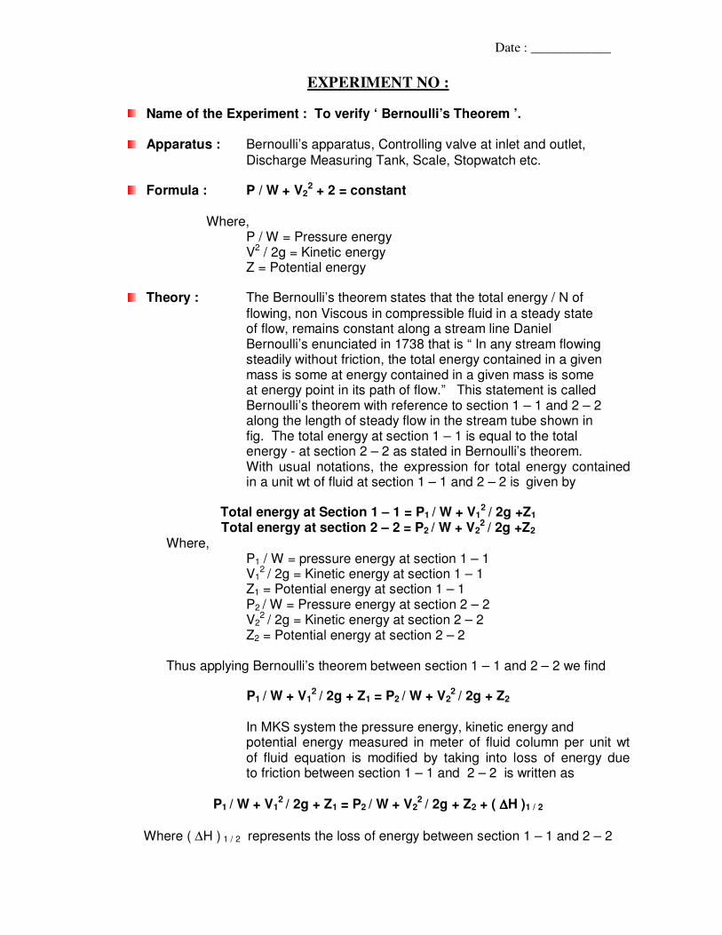
Observation : 1) Area of collecting tank = A = L x B = cm2

2) Difference in water level in collecting tank = ∆h

3) Time required for rise of water level by 10 cm = ∆t 4) Discharge = Qact = Volume of water cm3/sec

Time

Observation Table :

Sr. No.

Piezometric head = P/W+Z

Duct area (a)

cm.

Velocity- V = Q/a cm/sec

V2/2g cm P / W + V2/2G + Z

01. 02. 03. 04. 05.

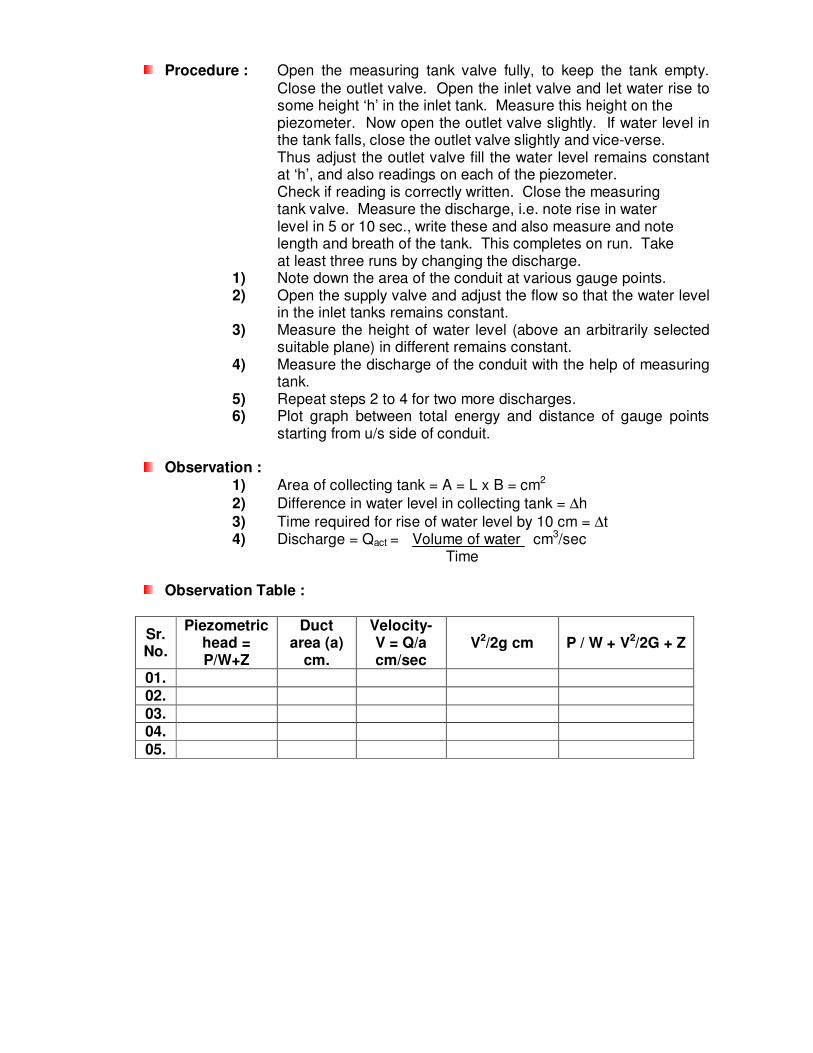
Sample Calculation : 1) Discharge = Qact = A x ∆∆∆∆h cm3/sec

∆∆∆∆t 2) Duct area = a = 4 x L cm2 3) Velocity = V = Q/a cm/sec 4) Velocity head = V2/2g cm 5) Total head = P / W + V2/2G + Z 6) Draw the graph - a) No. of tubes to –

P/W+Z b) No. of tubes to - V2/2g cm c) No. of tubes to - P / W + V2/2G + Z

Result : The total energy of a streamline, while the particle moves from one point to another. Bernoulli’s theorem for an incompressible fluid flow is verified.

Date : ____________

EXPERIMENT NO :

Name of the Experiment : To determine the Friction Factor ‘ F ’ for a pipe.

Apparatus : U – tube manometer connected across a pipe line, Stop

Watch, Collecting tank etc.

Formula : Head loss due to friction in pipe

hf = 4flv2 OR Flv2

2gd 2gd

Where : F = friction factor = (4f) l = length of pipe V = Velocity of flow through pipe. d = Diameter of pipe. g = Acceleration due to gravity. f = Coeff. of friction

Theory : The experimental set up consists of a large number of pipes

of different diameters. The pipes have tapping at certain distance so that a U – Tube manometer is connected in between them. The flow of water through a pipeline is regulated by operating a control valve which is provided in main supply line, for measuring the head loss. The length of the pipe is considered as a distance between the two pressure tapping, to which a U – Tube mercury manometer is fitted. Actual discharge through pipeline is calculated by collecting the water in collecting tank and by noting the time for collection. ∴ Velocity of flow = V = Q = ( A ���� H ) / t a a

Where : A = Area of tank. H = Depth of water collected in tank. t = Time required to collect the water up to a height “H” in the tank. a = Area of pipe. Q = Discharge through pipe. Now applying Bernoulli’s equation between two pressure tapping, we have.

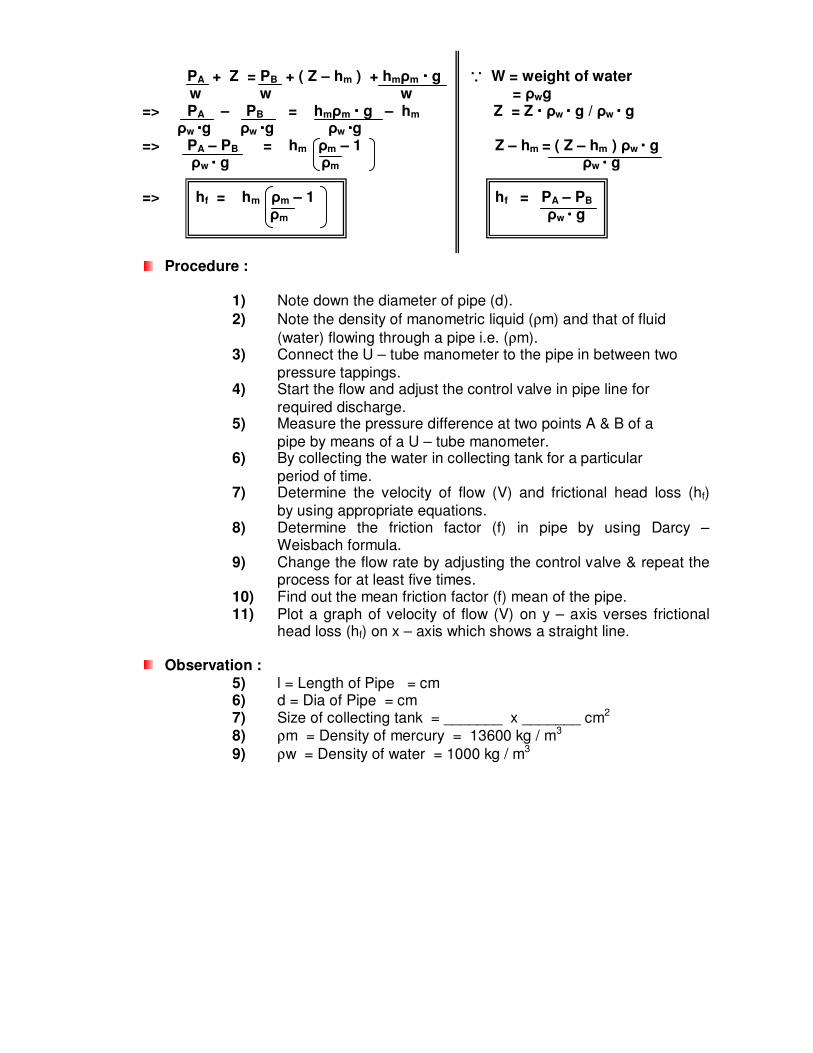
PA + Z = PB + ( Z – hm ) + hmρm ���� g ∵ ∵ ∵ ∵ W = weight of water w w w = ρwg => PA – PB = hmρm ���� g – hm Z = Z ���� ρw ���� g / ρw ���� g ρw ����g ρw ����g ρw ����g => PA – PB = hm ρm – 1 Z – hm = ( Z – hm ) ρw ���� g ρw ���� g ρm ρw ���� g => hf = hm ρm – 1 hf = PA – PB ρm ρw ���� g

Procedure : 1) Note down the diameter of pipe (d).

2) Note the density of manometric liquid (ρm) and that of fluid

(water) flowing through a pipe i.e. (ρm). 3) Connect the U – tube manometer to the pipe in between two

pressure tappings. 4) Start the flow and adjust the control valve in pipe line for

required discharge. 5) Measure the pressure difference at two points A & B of a

pipe by means of a U – tube manometer. 6) By collecting the water in collecting tank for a particular

period of time. 7) Determine the velocity of flow (V) and frictional head loss (hf)

by using appropriate equations. 8) Determine the friction factor (f) in pipe by using Darcy –

Weisbach formula. 9) Change the flow rate by adjusting the control valve & repeat the

process for at least five times. 10) Find out the mean friction factor (f) mean of the pipe. 11) Plot a graph of velocity of flow (V) on y – axis verses frictional

head loss (hf) on x – axis which shows a straight line.

Observation : 5) l = Length of Pipe = cm 6) d = Dia of Pipe = cm 7) Size of collecting tank = _______ x _______ cm2 8) ρm = Density of mercury = 13600 kg / m3

9) ρw = Density of water = 1000 kg / m3

Observation Table :

Sr. No.

Manometic Reading Tank Reading

Left Limb

Right Limb

Diff. (hB - hA)

Initial height

Final height

Diff H2-H1

HA cm

HB cm

hm cm

Frictional Head Loss

hf=hm ρm – 1

ρw

hf = PA – PB

ρw .g

Meter

H1 cm

H2 cm

H

cm

Time

t

Sec

Actual Discharge

Qac= AH t

M3/Sec

Velocity of flow

V = Qac a

M/Sec

frict-ion

factor F

fmean

01. 02.

03.

04. 05.

Sample Calculation : 1) a = c/s area of pipe

= π (d)2 = π ( )2 = ______ M2

4 4 7) A = Area of tank = _______ x _________

For Reading No. 1

Frictional head loss = hf = hm ρρρρm – 1

ρρρρw = ______ 13600 – 1 1000 Actual Discharge Qac = AH = ____x_____ t = ______ M3 / Sec Velocity of flow V = Qac / a = _____ = _____ m / Sec Friction factor F = 2hf.g.d lv2 OR Coeff. of friction f = 2hf.g.d = hf.gd 4.l.v2 2lv2 Mean friction factor fmean

Result : The friction factor “ F ” for the pipe is found to be ________.

Date : ____________

EXPERIMENT NO :

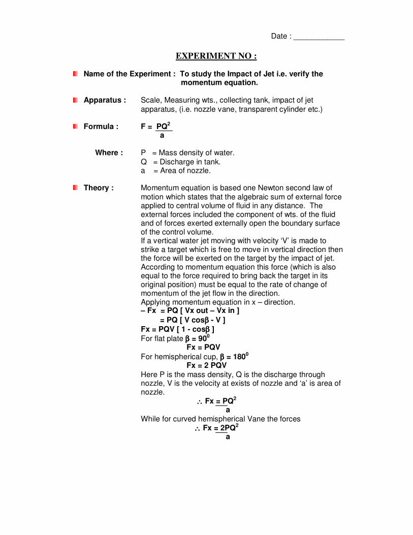
Name of the Experiment : To study the Impact of Jet i.e. verify the momentum equation.

Apparatus : Scale, Measuring wts., collecting tank, impact of jet

apparatus, (i.e. nozzle vane, transparent cylinder etc.)

Formula : F = PQ2 a

Where : P = Mass density of water.

Q = Discharge in tank. a = Area of nozzle.

Theory : Momentum equation is based one Newton second law of motion which states that the algebraic sum of external force applied to central volume of fluid in any distance. The external forces included the component of wts. of the fluid and of forces exerted externally open the boundary surface of the control volume. If a vertical water jet moving with velocity ‘V’ is made to strike a target which is free to move in vertical direction then the force will be exerted on the target by the impact of jet. According to momentum equation this force (which is also equal to the force required to bring back the target in its original position) must be equal to the rate of change of momentum of the jet flow in the direction. Applying momentum equation in x – direction. – Fx = PQ [ Vx out – Vx in ]

= PQ [ V cosββββ - V ]

Fx = PQV [ 1 - cosββββ ]

For flat plate ββββ = 900 Fx = PQV

For hemispherical cup, ββββ = 1800 Fx = 2 PQV

Here P is the mass density, Q is the discharge through nozzle, V is the velocity at exists of nozzle and ‘a’ is area of nozzle.

∴∴∴∴ Fx = PQ2 a

While for curved hemispherical Vane the forces ∴∴∴∴ Fx = 2PQ2

a

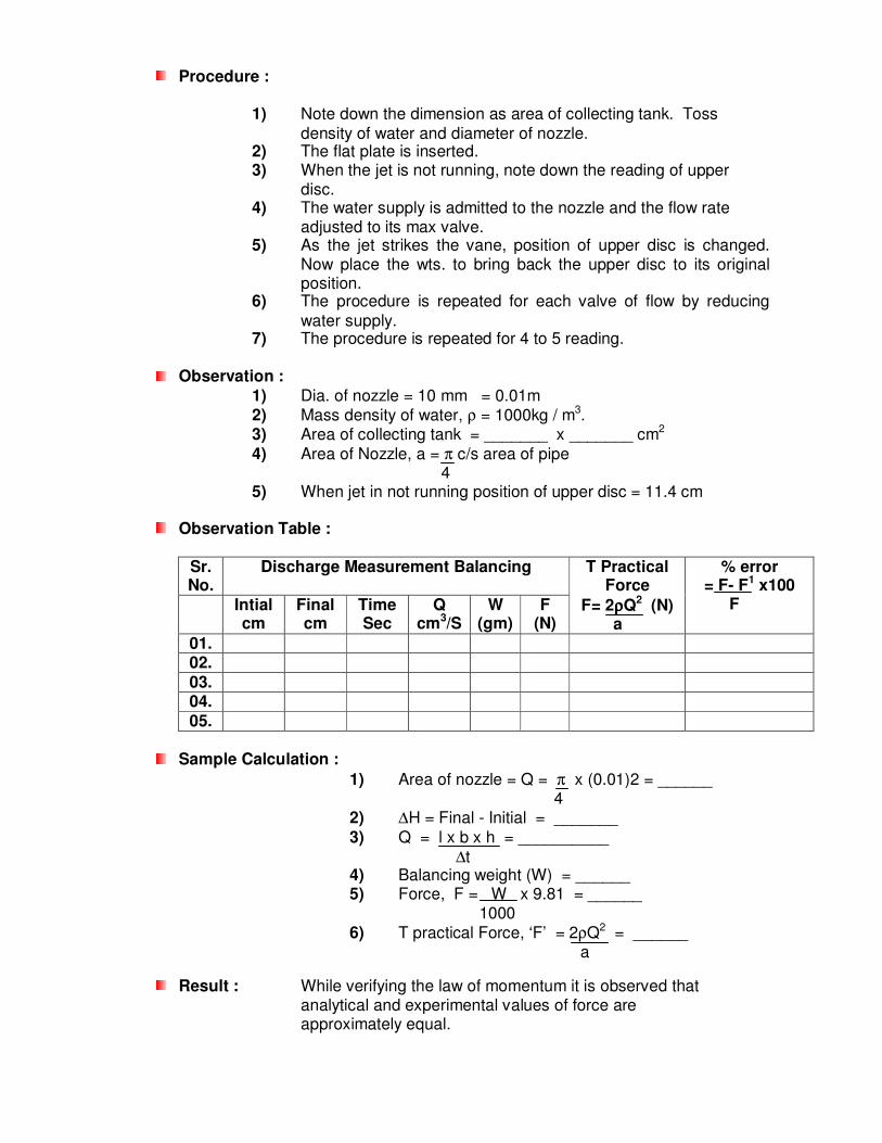
Procedure :

1) Note down the dimension as area of collecting tank. Toss

density of water and diameter of nozzle. 2) The flat plate is inserted. 3) When the jet is not running, note down the reading of upper disc. 4) The water supply is admitted to the nozzle and the flow rate adjusted to its max valve. 5) As the jet strikes the vane, position of upper disc is changed. Now place the wts. to bring back the upper disc to its original position. 6) The procedure is repeated for each valve of flow by reducing

water supply. 7) The procedure is repeated for 4 to 5 reading.

Observation :

1) Dia. of nozzle = 10 mm = 0.01m 2) Mass density of water, ρ = 1000kg / m3. 3) Area of collecting tank = _______ x _______ cm2

4) Area of Nozzle, a = π c/s area of pipe 4

5) When jet in not running position of upper disc = 11.4 cm

Observation Table :

Sr. No.

Discharge Measurement Balancing

Intial cm

Final cm

Time Sec

Q cm3/S

W (gm)

F (N)

T Practical Force

F= 2ρρρρQ2 (N) a

% error = F- F1 x100

F

01. 02.

03. 04.

05.

Sample Calculation :

1) Area of nozzle = Q = π x (0.01)2 = ______ 4 2) ∆H = Final - Initial = _______

3) Q = l x b x h = __________

∆t 4) Balancing weight (W) = ______ 5) Force, F = W x 9.81 = ______

1000

6) T practical Force, ‘F’ = 2ρQ2 = ______ a

Result : While verifying the law of momentum it is observed that analytical and experimental values of force are approximately equal.

Date : ____________

EXPERIMENT NO :

Name of the Experiment : Determination of coefficient of discharge, coefficient of contraction, coefficient of velocity on orifice.

Apparatus : Intel tank which is fed from on overhead tank through a pipe

network sharp edge orifice, hock gauge attached to the inlet tank, Stop watch, Scale etc.

Formula : Qtn = a x √√√√ 2gh

Qac = V = A . ∆∆∆∆H t t

Where : a = Area of orifice. Q = Constant head of water in inlet tank. V = Volume of water collected in tank.

A = C / S area of tank.

∆H = Depth of water collected in tank. t = Time require to collect the water in collecting tank.

Theory : Orifice is a small opening of any U / S such as circular,

triangular, rectangular, on a side or on the bottom of the tank, through which a fluid flows. Orifices are used for measuring he rate of flowing fluid. The water is allowed to flow through an orifice fitted to tank and a constant head ‘H’. The water is collected in measuring tank for known time ‘ t ‘. The height of water in the measuring tank is noted. Then the actual discharge through the orifice.

Qac = A x ∆∆∆∆H t

Qtn = a x √√√√ 2gh Cd = Qac

Qtn

Coefficient Velocity = Actual Velocity Theoretical Velocity

Consider a liquid particle which is at vena contract at any time status the position along the jet at P. Jet x = horizontal distance traveled by paticles y = vertical distance by particle. v = actual velocity of jet.

∴ Horizontal distance, x = v x t -- � Vertical distance g = ½ g t2 -- �

∴ from � and � g = ½ g x2 / V2

∴∴∴∴ = V2 = gx2 / 2g

∴∴∴∴ = V = gx2

2g

But theoretical velocity, Vtn = 2gh

∴∴∴∴ Cv = V Vtn

∴∴∴∴ Cv = gx2 x 1 = x2

2g 2g 4gH

Cc = Cd Cv

Procedure :

1) The dia of the orifice, dimension of measuring tank, and dia of pipeline were noted.

2) The x and y movement of the pointer was checked to be jerk free and smooth.

3) The inlet controlled valve was opened. The inlet tank was allowed to fill the over flow started. The inlet valve was from adjusted till the water level in the tank becomes constant as checked by piezometer reading.

4) After 3 to 5 min, when steady of flow acquired, it and valve of x and y were measured open pointer was kept at center of jet.

5) The discharge was measured and head ‘h’ was calculated again. The procedure was repeated for a set of 4 different reading.

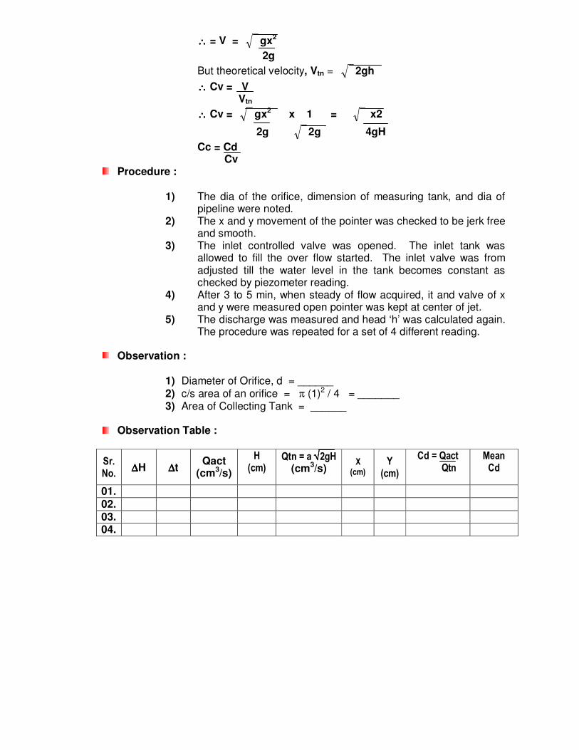
Observation :

1) Diameter of Orifice, d = ______ 2) c/s area of an orifice = π (1)2 / 4 = _______ 3) Area of Collecting Tank = ______

Observation Table :

Sr. No.

∆∆∆∆H ∆∆∆∆t Qact

(cm3/s)

H (cm)

Qtn = a √√√√2gH (cm3/s)

X (cm)

Y (cm)

Cd = Qact Qtn

Mean Cd

01.

02. 03. 04.

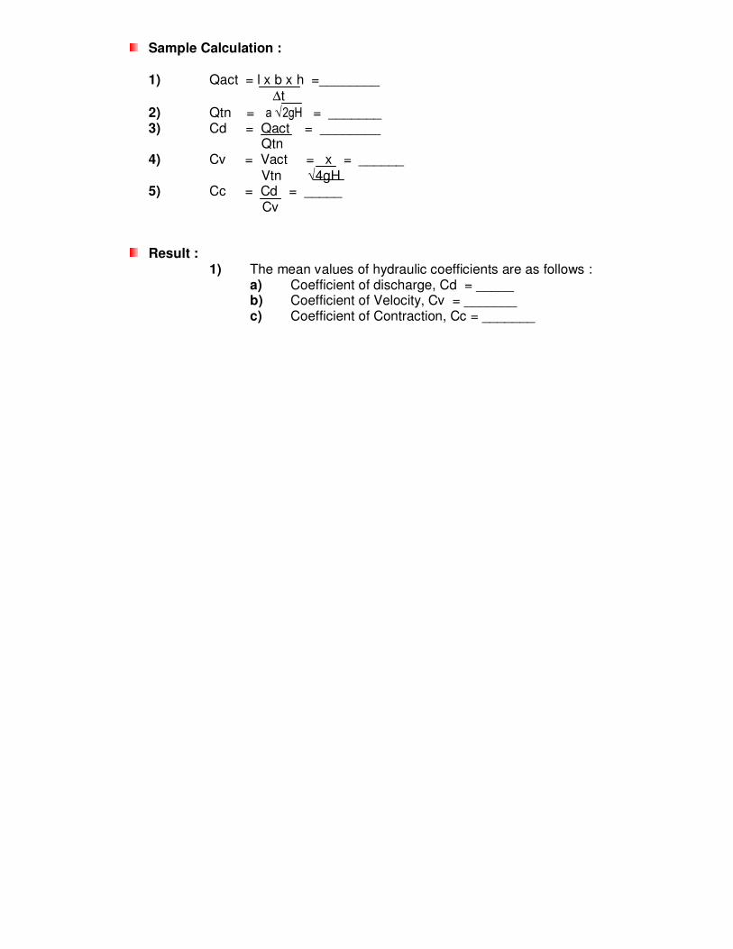
Sample Calculation :

1) Qact = l x b x h =________ ∆t

2) Qtn = a √2gH = _______ 3) Cd = Qact = ________ Qtn 4) Cv = Vact = x = ______

Vtn √4gH 5) Cc = Cd = _____ Cv

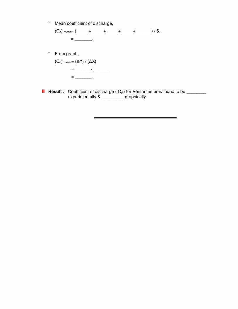
Result : 1) The mean values of hydraulic coefficients are as follows :

a) Coefficient of discharge, Cd = _____ b) Coefficient of Velocity, Cv = _______ c) Coefficient of Contraction, Cc = _______

Date :______________

EXPERIMENT NO :

Name of the Experiment : To determine the coefficient of discharge ( Cd )

for an Orificemeter.

Apparatus : An Orificemeter fitted across a pipeline leading to a collecting tank,

Stop Watch, U-Tube manometer etc.

Formula : Actual discharge through Orificemeter Q ac = C.a1.a0(2g.h)1/2 / [a1

2 – a02]1/2

Where: C : Constant i.e. Coefficient of Orificemeter. C = Cd .{1 – (a0

2 / a12)}1/2 / {1 – Cd

2(a02 / a1

2)}1/2 Cd : Coefficient of discharge for Orificemeter. a1 : Cross section area of pipe at inlet i.e. entry section. a0 : Cross section area of Orifice.

h : Pressure head difference in terms of fluid flowing through pipeline system.

Again, Actual discharge through Orificemeter Q ac = V / t = (A.∆H) / t

V : (A.∆H) i.e. Volume of water collected in collecting tank A : Cross section area of collecting tank. ∆H : (H2 – H1) i.e. Depth of water collected in collecting tank. t : Time required to collect the water up to a height ∆H in the collecting tank.

Theory : An Orificemeter is used to measure the discharge in a pipe. An Orificemeter in it’s simplest form consists of a plate having a sharp edged circular hole known as an orifice. The plate is fixed inside the pipe as shown in figure.

A mercury U-tube manometer is inserted to know the difference of pressure head between the two tapping. Orificemeter works on the same principle as that of Venturimeter i.e. by reducing the area of flow passage a pressure difference is developed between the two section and the measurement of pressure difference is used to find the discharge. By applying Bernoulli’s equation between inlet of pipe & throat i.e. orifice section.

(p1 / w) + (v12 / 2g) + z1 = (p2 / w) + (v2

2 / 2g) + z2

When Orificemeter is connected in horizontal pipe, then z1 = z2 Therefore (p1 - p2) / w = (v2

2 / 2g) - (v12 / 2g)

h = (v22 / 2g) - (v1

2 / 2g) -------------------------------------------- 1.

Further if a1 & a2 be the cross section area of Pipe at inlet & that of jet respectively, then by continuity equation

Q = a1v1 = a2v2

a2 = a1v1 / v2 ------------------------------------------------------- a

If Cc = Coefficient of contraction = a2 / a0

Cc = Area of jet at vena contracta / Area of orifice a2 = Cc a0 ------------------------------------------------------- b

v1 = Cc v2 (a0 / a1) From equation 1; v2 = ( 2gh + v1

2 )1/2 in this equation losses has not been considered and gives theoretical velocity. v2 = ( 2gh + v1

2 )1/2

If Cv= Coefficient of velocity = Actual velocity / Theorotical velocity ∴Actual velocity of jet at vena contracta i.e. at section 2 v2 = Cv ( 2gh + [Cc v2 (a0 / a1)]

2 )1/2

v2 = Cv {(2gh )1/2 /(1- [Cc Cv (a0 / a1)] 2 )1/2 }

But Coefficient of discharge Cd = Cc Cv By continuity equation Q = a2v2

Q = Cc a0 v2

Q = Cc Cv a0 {(2gh )1/2 /(1- [Cc Cv (a0 / a1)] 2 )1/2 }

Q = Cd a0 {(2gh )1/2 /(1- [Cd (a0 / a1)] 2 )1/2 }

If C= Constant of orificemeter, then

C = Cd {1 – (a02 / a1

2)}1/2 / {1 – Cd2(a0

2 / a12)}1/2

Q ac = C.a0(2g.h)1/2 / {1 – (a0

2 / a12)}1/2

Q ac = C.a1.a0(2g.h)1/2 / (a12 – a0

2)1/2

Procedure :

* Note the diameter at the inlet of pipe (d1) and the diameter of an orifice (do).

* Note the density of manometric liquid i.e. mercury (ρm) and that of fluid flowing

through pipeline i.e. water (ρw).

* Connect the U-tube manometer to the pressure toppings of orificemeter, one

end at the inlet section and the other end at the section where jet of water

leaves from orifice forming a vena contracta.

* Start the flow and adjust the control valve in pipeline to get the required

discharge.

* Measure the pressure difference (Hm) between two sections of orificemeter by

using U - tube mercury manometer.

* Convert the pressure head difference in meters of fluid flowing through

pipeline ( i.e. water ) by using the equation h = Hm [(ρm / ρw) -1]

* Measure flow rate i.e. actual discharge (Qac) through Venturimeter by means

collecting the water in collecting tank for a specified period of time.

Q ac = V / t = (A.∆H) / t

* Change the flow rate by adjusting the control valve and repeat the process or

at least five times.

* Determine the constant (C) of orificemeter and then calculate coefficient of

discharge (Cd) for each flow rate and find the mean value of coefficient of

discharge (Cd) mean.

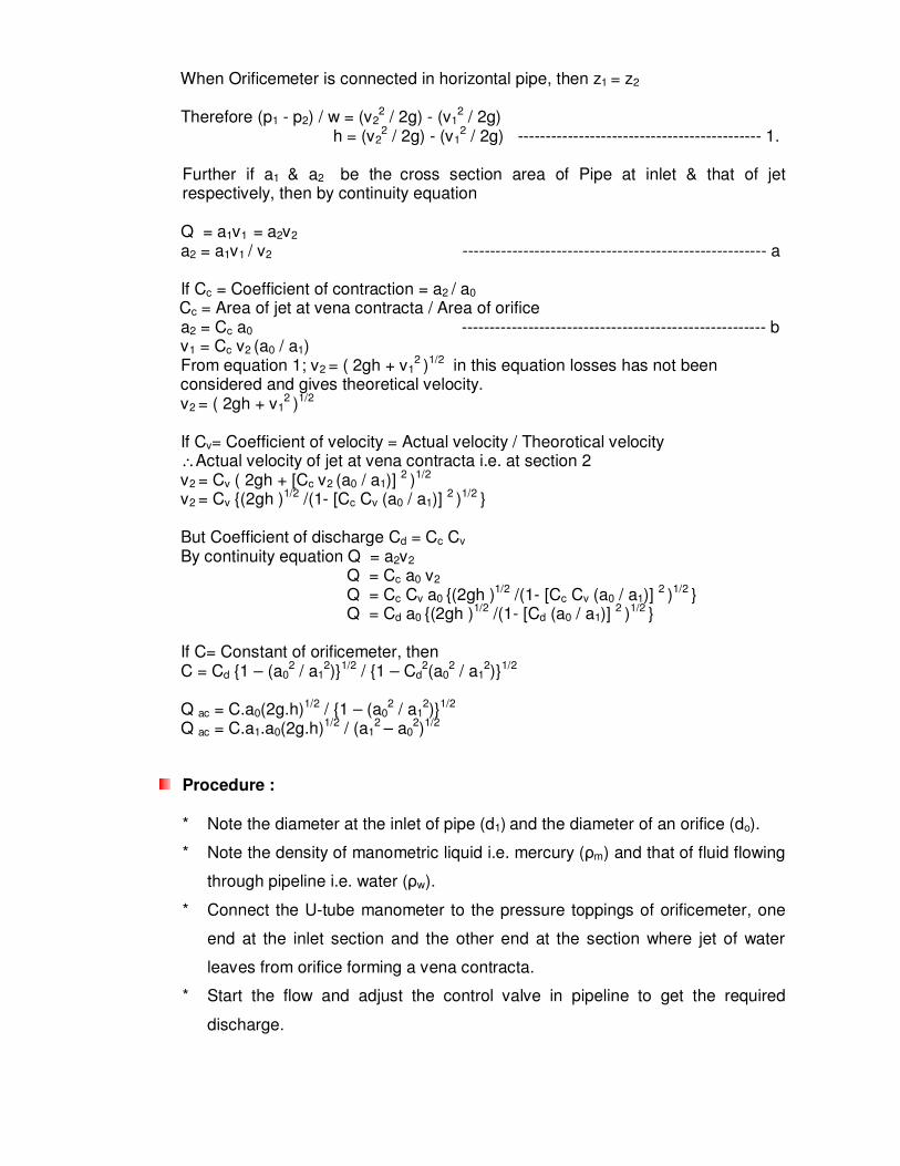
Observation :

Diameter of pipe, d1 = ______ m

Diameter of orifice, do = ______ m

Area of collecting tank, A = ______x______ = ________ m2

Area of pipe at entry, a1 = [(л/4) d12] = [(л/4) ( )2] = ________ m2.

Area of orifice, ao = [(л/4) do2] = [(л/4) ( )2] = ________ m2.

Density of mercury, ρm =13600 kg / m3.

Density of water, ρw =1000 kg / m3

Observation Table :

Manometric Reading

Pressure Head Diff.

Tank Reading

Actual Discharge

Left Limb

Right Limb

Diff. h2 - h1

h = Hm[(ρm/ρw) -1]

Initial

Final Diff. H2 - H1

Time t

Q ac = (A.∆H) / t

Sr. No.

h1 m

h2 m

Hm

m m

H1 m

H2

m ∆H m

sec m3 / sec

Constant of Orificemeter

C =

Qac [a12 – a02]1/2

[a1.a0( 2g.h )1/2]

Coefficient of

Discharge

Cd

1

2

3

4

5

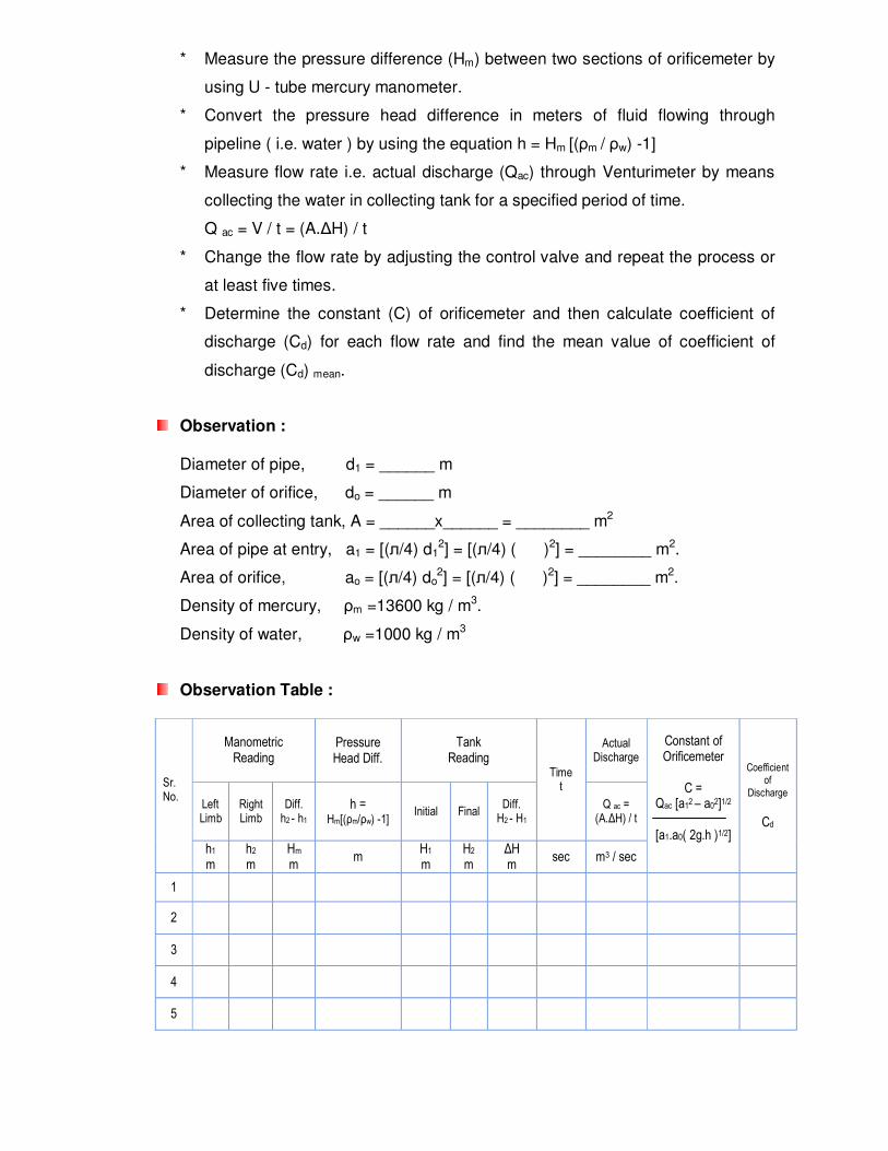
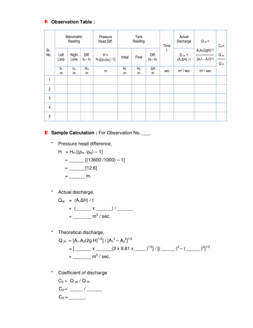
Sample Calculation : For Observation No. ___.

* Pressure head difference,

h = Hm [(ρm /ρw) – 1]

= ______ [(13600 /1000) – 1]

= ______ [12.6]

= ______ m.

* Actual discharge,

Qac = (A.∆H) / t

= (______ x ______) / ______

= _______ m3 / sec.

* Constant of Orificemeter, C = Qac [a1

2 – a02]1/2 / [a1.a0( 2g.h )1/2]

= ______ [ _____2 – _____2 ]1/2 / [ _____ x _____( 2 x 9.81 x ______ )1/2]

= ___________ / __________

= __________

* To Find Coefficient of Discharge (Cd),

By Using Relation

C = Cd .{1 – (a02 / a1

2)}1/2 / {1 – Cd2(a0

2 / a12)}1/2

_______ = Cd .{1 – ( _____2 / _____2)}1/2 / {1 – Cd2(______2 / _______2)}1/2

∴

Cd = _________

* Mean Constant of Orificemeter,

(C) mean = ( ____ +_____+_____+_____+______ ) / 5.

= _______.

* Mean Coefficient of Discharge for Orificemeter,

(Cd) mean = ( ____ +_____+_____+_____+______ ) / 5.

= _______.

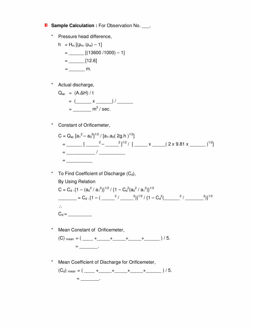
Result :

* Constant of orificemeter ( C ) is found to be ________ * Coefficient of discharge for orificemeter (Cd) is found to be ________

Date : ____________

EXPERIMENT NO :

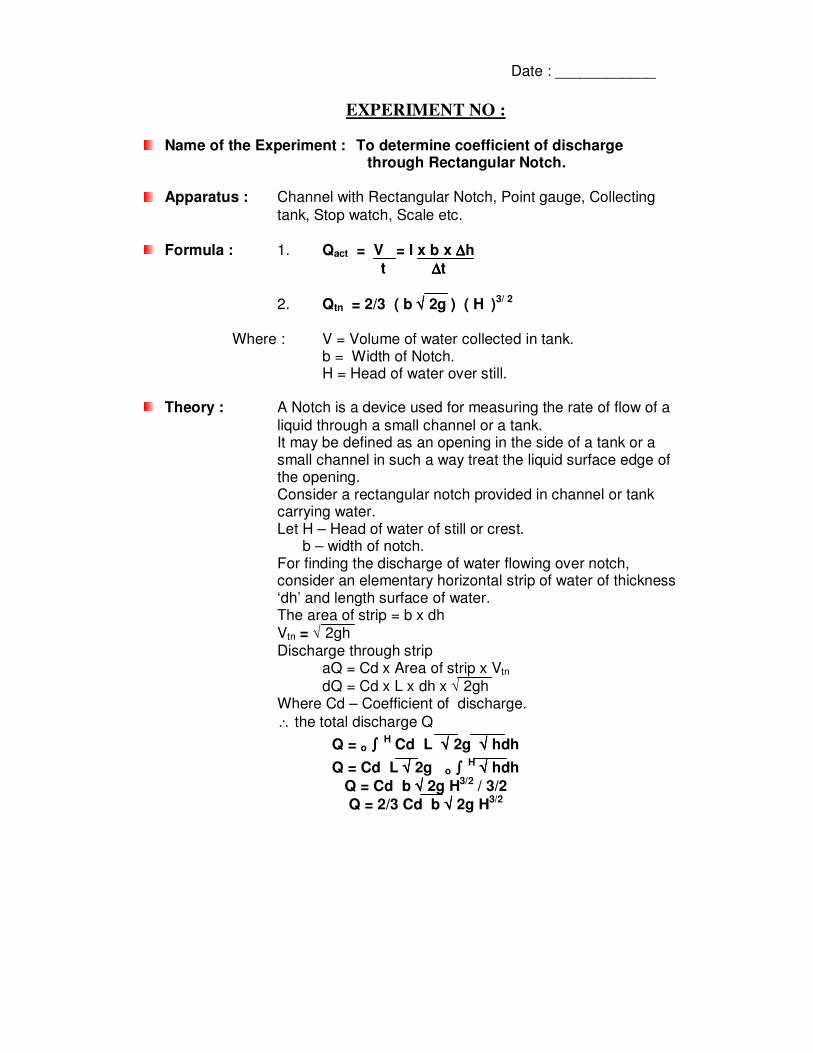
Name of the Experiment : To determine coefficient of discharge through Rectangular Notch.

Apparatus : Channel with Rectangular Notch, Point gauge, Collecting

tank, Stop watch, Scale etc.

Formula : 1. Qact = V = l x b x ∆∆∆∆h

t ∆∆∆∆t

2. Qtn = 2/3 ( b √√√√ 2g ) ( H )3/ 2 Where : V = Volume of water collected in tank. b = Width of Notch. H = Head of water over still.

Theory : A Notch is a device used for measuring the rate of flow of a

liquid through a small channel or a tank. It may be defined as an opening in the side of a tank or a small channel in such a way treat the liquid surface edge of the opening. Consider a rectangular notch provided in channel or tank carrying water. Let H – Head of water of still or crest. b – width of notch. For finding the discharge of water flowing over notch, consider an elementary horizontal strip of water of thickness ‘dh’ and length surface of water. The area of strip = b x dh Vtn = √ 2gh Discharge through strip aQ = Cd x Area of strip x Vtn

dQ = Cd x L x dh x √ 2gh Where Cd – Coefficient of discharge.

∴ the total discharge Q

Q = o ∫∫∫∫ H Cd L √√√√ 2g √√√√ hdh

Q = Cd L √√√√ 2g o ∫∫∫∫ H √√√√ hdh

Q = Cd b √√√√ 2g H3/2 / 3/2

Q = 2/3 Cd b √√√√ 2g H3/2

Procedure :

1) The tank dimensions were measured. 2) The flow in the off was started. 3) The flow was kept constant. 4) The head of water in piezometer of constant time interval for

collecting tank was noted. 5) Open slightly the valve without increase the rotation suddenly after

fixed time interval. 6) Also note the head over the still after each interval.

Observation :

1) Volume of tank = 2) Width of rectangular Notch = b =

3) Time ∆ t = constant =

Observation Table :

Point Gauge Reading Discharge measurement Sr. No.

Initial (cm)

Final (cm)

Diff. (H) (cm)

∆∆∆∆R (cm)

∆∆∆∆t (sec)

Qact = v t (cm3 / s)

Cd = Qact

2 / 3 (b √√√√ 2g )(H 3) / 2

01. 02.

03. 04.

Sample Calculation :

1) V =

2) Qact = V/t =

3) Qtn = 2 / 3 (b √ 2g )(H 3) / 2 4) Cd = Qact =

2 / 3 (b √ 2g )(H 3) / 2

Result : Coefficient of discharge for rectangular notch was found to

be _________

Date : ____________

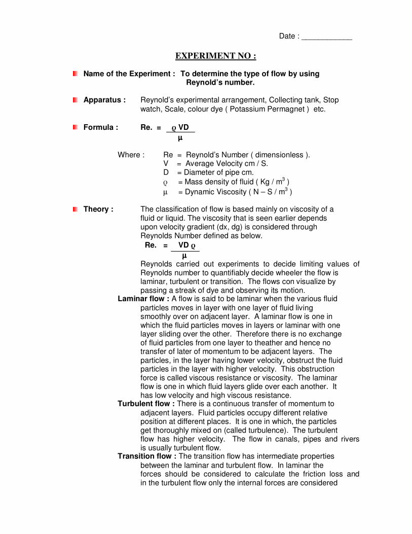
EXPERIMENT NO :

Name of the Experiment : To determine the type of flow by using Reynold’s number.

Apparatus : Reynold’s experimental arrangement, Collecting tank, Stop

watch, Scale, colour dye ( Potassium Permagnet ) etc.

Formula : Re. = ρ VD

µµµµ Where : Re = Reynold’s Number ( dimensionless ). V = Average Velocity cm / S. D = Diameter of pipe cm.

ρ = Mass density of fluid ( Kg / m3 )

µ = Dynamic Viscosity ( N – S / m3 )

Theory : The classification of flow is based mainly on viscosity of a fluid or liquid. The viscosity that is seen earlier depends upon velocity gradient (dx, dg) is considered through Reynolds Number defined as below.

Re. = VD ρ

µµµµ Reynolds carried out experiments to decide limiting values of Reynolds number to quantifiably decide wheeler the flow is laminar, turbulent or transition. The flows con visualize by passing a streak of dye and observing its motion. Laminar flow : A flow is said to be laminar when the various fluid

particles moves in layer with one layer of fluid living smoothly over on adjacent layer. A laminar flow is one in which the fluid particles moves in layers or laminar with one layer sliding over the other. Therefore there is no exchange of fluid particles from one layer to theather and hence no transfer of later of momentum to be adjacent layers. The particles, in the layer having lower velocity, obstruct the fluid particles in the layer with higher velocity. This obstruction force is called viscous resistance or viscosity. The laminar flow is one in which fluid layers glide over each another. It has low velocity and high viscous resistance. Turbulent flow : There is a continuous transfer of momentum to

adjacent layers. Fluid particles occupy different relative position at different places. It is one in which, the particles get thoroughly mixed on (called turbulence). The turbulent flow has higher velocity. The flow in canals, pipes and rivers is usually turbulent flow. Transition flow : The transition flow has intermediate properties

between the laminar and turbulent flow. In laminar the forces should be considered to calculate the friction loss and in the turbulent flow only the internal forces are considered

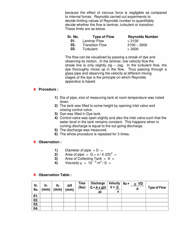
because the effect of viscous force is negligible as compared to internal forces. Reynolds carried out experiments to decide limiting values of Reynolds number to quantifiably decide whether the flow is laminar, turbulent or transition. These limits are as below.

Sr. No. Type of Flow Reynolds Number 01. Laminar Flow < 2100 02. Transition Flow 2100 – 3000 03. Turbulent > 3000

The flow can be visualized by passing a streak of dye and observing its motion. In the laminar, low velocity flow the streak line is only slightly zig – zag. In the turbulent flow, the dye thoroughly mixes up in the flow. Thus passing through a glass pipe and observing the velocity at different mixing stages of the dye is the principle on which Reynolds apparatus is based.

Procedure :

1) Dia of pipe, size of measuring tank at room temperature was noted

down. 2) The tank was filled to some height by opening inlet valve and

closing control valve. 3) Dye was filled in Dye tank. 4) Control valve was open slightly and also the inlet valve such that the

water level in the tank remains constant. This happens when in coming discharge is equal to the out going discharge.

5) The discharge was measured. 6) The whole procedure is repeated for 3 times.

Observation :

1) Diameter of pipe = D =

2) Area of pipe = G = π / 4 (25)2 = 3) Area of Collecting Tank = A =

4) Viscosity µ = 10 – 5 m2 / S =

Observation Table :

Sr. No.

H1

(mm) H2

(mm) ∆∆∆∆H

(mm)

Time (Sec)

Discharge

Q = A x ∆∆∆∆H

∆∆∆∆t

Velocity V = Q a

Re = ρ VD

µµµµ Type of Flow

01.

02. 03.

04.

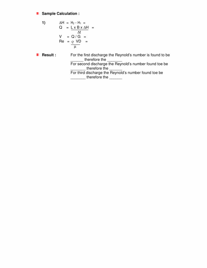
Sample Calculation :

1) ∆H = H2 - H1 =

Q = L x B x ∆H =

∆t V = Q / G =

Re = ρ VD =

µ

Result : For the first discharge the Reynold’s number is found to be

______ therefore the _______ For second discharge the Reynold’s number found toe be _______ therefore the ______ For third discharge the Reynold’s number found toe be _______ therefore the ______

Date : ____________

EXPERIMENT NO :

Name of the Experiment : To determine loss of head & power Loss due to Sudden Expansion and Sudden Contraction.

Apparatus : Pipe of smaller diameter connected to larger diameter, inlet,

outlet valves, collecting tank, stopwatch etc.

Formula : Losses due to

1. Sudden Expansion he = (V1 – V2) 2g Where : he = Loss of head due to sudden expansion. V1 = Velocity of flow at smaller section. V2 = Velocity of flow at larger Section.

2. Sudden Contraction hc = 0.5 V2

2 2g

Where : hc = Loss of head due to sudden contraction.

Theory : Loss of energy duet to change of velocity of the flowing fluid in magnitude or direction is called as minor loss of energy. Loss of head due to Sudden Expansion : Consider a fluid flowing through a pipe line which has sudden enlargement. Consider two section 1 – 1 and 2 – 2 before and after enlargement. Let; P1 = Pressure intensity at section 1 – 1. V1 = Velocity of flow at section 1 – 1. A1 = Area of pipe at section 1 – 1. P2, V2 and A2 = Corresponding at section 2 – 2. Due to sudden change of diameter, the liquid flowing from smaller pipe is not able to fallow abrupt change of boundary and turbulent eddies are formed, since the flow separates from the boundary. Let P1 = Pressure intensity of the liquid eddies on Area A2 – A1, he = Loss of head due to expansion. Applying Bernoulli’s equation at section 1 – 1 and 2 – 2.

P1 + V12 + Z1 = P2 + V2

2 + Z2 + he W 2g W 2g But Z1 = Z2

∴ he = P1 - P2 + V12 - V2

2 -- �

W W 2g 2g Consider the control volume of liquid between 2 sections.

Fx = P1 A1 + P1 (A2 - A1) P2 A2 = ( P1 - P2 ) A2 -- � Momentum of liquid / Sec at Section 1 –1 = mass x Velocity

= � A1 V1·V1

= � A1 V12

Similarly at section 2 – 2 = � A2 V22

∴ Change of momentum / Sec = � A2 V22 – � A2 V2 x V1

2

= � A2 (V22 – V1 V2) -- �

Net force acting on the control vol. in the direction of flow must be equal to the rate of change of momentum per

second. Hence equating � and �.

( P1 - P2 ) A2 = � A2 (V22 – V1 V2)

∴ P1 - P2 = V22 – V1 V2

� Dividing throughout by g P1 - P2 = V2

2 – V1 V2 OR P1 - P2 = V22 – V1 V2

� g g W W g

Substituting in equation �

he = V22 - V1 V2 + V1

2 - V22

g 2g 2g On solving he = ( V1

2 - V2 )2

2g Loss of head due to Sudden Contraction : Consider a liquid flowing in a pipe which has a sudden contraction in area. Consider tow section 1 – 1 and 2 – 2, before and after contraction. As the fluid flows from larger pipe to smaller pipe, the area of flow goes on decreasing and becomes minimum at section C – C. This section is called venacontract. After section C – C sudden enlargement takes place. The loss of head duet to sudden enlargement from Vena-contract to smaller pipe. Let; Ac = area of flow at Vena-contract Vc = Velocity of flow at Vena-contract A2 = area of flow at section 2 – 2 V2 = Velocity of flow at section 2 – 2

hc = Loss of head due to sudden expansion. Now, hc = actually loss of head due to enlargement from Vena- contract to section 2 – 2 and is given by

hc = (Vc – V2 )2

= V2 Vc – 1

2g V2

From continuity equation; AC VC = A2 V2 i .e.

VC = AC = 1 = 1

V2 = A2 = AC/A2 = CC

Substituting in equation -- 1

hc = V22 1 – 1

2g CC

If valve of CC is not given, then the head loss due to contraction is given as

hC = 0.5 V22

2g Procedure :

1) Arrange and check the apparatus as shown in fig. 2) Measure diameter of pipe and dimensions of measuring tank and

record. 3) Open the inlet valve, keeping the outlet valve opened. 4) Connections of the manometer sudden talings to one of the pipes /

pipe fittings and check that there is no air bubble entrapped. 5) Open partially the outlet valve, keeping the common inlet valve fully

open. 6) Let the flow become constant and take the readings. 7) Open both the valves, slightly about 2 mins. Open the pressure

tappin and wait till mercury surface in both limbs of the manometer becomes constant or still. Take readings of each limb, record and check.

8) Collect the discharge and measure the time require to fill up to 5 cm. 9) Simultaneously take manometer reading. Repeat procedure up to 6

to 7 times.

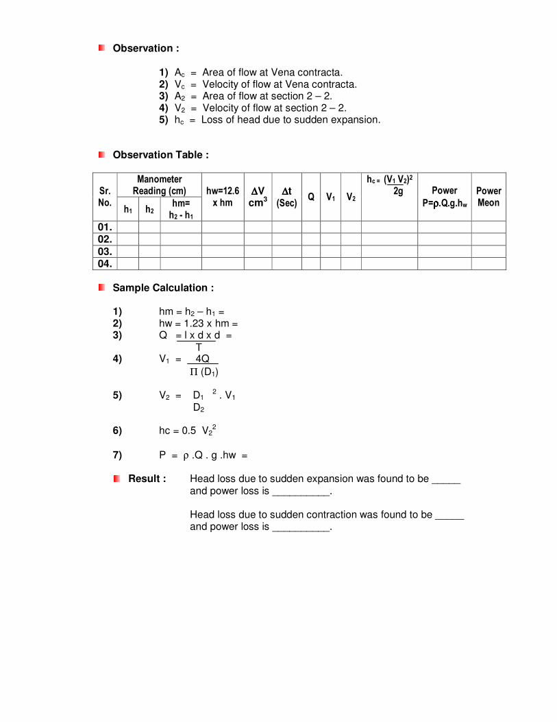
Observation :

1) Ac = Area of flow at Vena contracta. 2) Vc = Velocity of flow at Vena contracta. 3) A2 = Area of flow at section 2 – 2. 4) V2 = Velocity of flow at section 2 – 2. 5) hc = Loss of head due to sudden expansion.

Observation Table :

Manometer Reading (cm) Sr.

No. h1 h2

hm= h2 - h1

hw=12.6 x hm

∆∆∆∆V cm3

∆∆∆∆t (Sec)

Q V1 V2

hc = (V1 V2)2 2g Power

P=ρρρρ.Q.g.hw Power Meon

01. 02.

03. 04.

Sample Calculation : 1) hm = h2 – h1 = 2) hw = 1.23 x hm =

3) Q = l x d x d =

T 4) V1 = 4Q

Π (D1) 5) V2 = D1

2 . V1 D2 6) hc = 0.5 V2

2

7) P = ρ .Q . g .hw =

Result : Head loss due to sudden expansion was found to be _____ and power loss is __________. Head loss due to sudden contraction was found to be _____ and power loss is __________.

Date : ____________

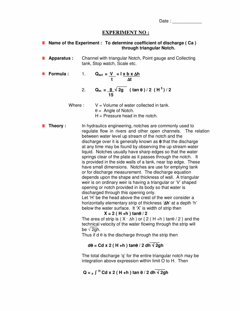
EXPERIMENT NO :

Name of the Experiment : To determine coefficient of discharge ( Ca ) through triangular Notch.

Apparatus : Channel with triangular Notch, Point gauge and Collecting

tank, Stop watch, Scale etc.

Formula : 1. Qact = V = l x b x ∆∆∆∆h

t ∆∆∆∆t

2. Qtn = 8 √√√√ 2g ( tan θθθθ ) / 2 ( H 5 ) / 2 15

Where : V = Volume of water collected in tank.

θ = Angle of Notch. H = Pressure head in the notch.

Theory : In hydraulics engineering, notches are commonly used to regulate flow in rivers and other open channels. The relation between water level up stream of the notch and the

discharge over it is generally known as θθθθ that the discharge at any time may be found by observing the up stream water liquid. Notches usually have sharp edges so that the water springs clear of the plate as it passes through the notch. It is provided in the side walls of a tank, near top edge. These have small dimensions. Notches are use for emptying tank or for discharge measurement. The discharge equation depends upon the shape and thickness of wall. A triangular weir is on ordinary weir is having a triangular or ‘V’ shaped opening or notch provided in its body so that water is discharged through this opening only. Let ‘H’ be the head above the crest of the weir consider a

horizontally elementary strip of thickness ‘∆∆∆∆h’ at a depth ‘h’ below the water surface. It ‘X’ is width of strip then

X = 2 ( H +h ) tanθθθθ / 2

The area of strip is ( X � ∆h ) or { 2 ( H +h ) tanθ / 2 } and the technical velocity of the water flowing through the strip will

be √ 2gh.

Thus if d θ is the discharge through the strip then

dθθθθ = Cd x 2 ( H +h ) tanθθθθ / 2 dh √√√√ 2gh The total discharge ‘q’ for the entire triangular notch may be integration above expression within limit O to H. Then

Q = a ∫∫∫∫ H Cd x 2 ( H +h ) tan θθθθ / 2 dh √√√√ 2gh

Assuming coefficient Cd to be constant for entire notch were obtain.

Q = Cd x 2 ( H +h ) tan θθθθ / 2 a ∫∫∫∫ H h1/2dh

Q = Cd x 2 ( H +h ) tan θθθθ / 2 [ 2/3 H h3/2 – 2/5 h5/2 ]HO

Q = 8/15 cd √√√√ 2g tan θθθθ / 2 H5/2

If the vector angle θθθθ equal to 900 then for θ/2 = 450 and θ/2 = 1

Q = 8/15 cd √√√√ 2g H5/2 For Cd assumed to be 0.6 then, Q = 1.418 H5/2 For discharge it is simplified as Q = KH5/2 Where K is constant for Notch

K = 8/15 Cd √√√√ 2g tan θθθθ / 2 Procedure :

1) Length and breadth of measuring tank is measured, also angle of

triangular Notch is measured. 2) Waste valve of the opening is open, then the inlet valve is slightly

open, were the flow over the still just starts, the inflow is stop. When this overflow stops fully, the initial gauge reading is measured.

3) The inlet valve is slightly open with the jerk. When the constant level is a acquired final gauge reading is recorded.

4) The discharge is then measured in the collecting tank. 5) The same procedure was repeated for at least 5 times.

Observation :

Angle of Notch = Q/2 = tan-1. Volume of tank =

Time ∆ t = constant =

Observation Table :

Point Gauge Reading Discharge measurement Sr. No.

Initial (cm)

Final (cm)

Diff. (H) (cm)

∆∆∆∆R ∆∆∆∆t Qact = LxBx∆∆∆∆h

t

Cd = Qact

8 / 15 ( tan θθθθ) / 2 ( H5 ) / 2

01. 02.

03.

04.

Sample Calculation :

1) V =

2) Qact = V / t =

3) Qtn = (8/15) √2g tan θ/2 H5/2 4) Cd = Qact =

Qtn

Result : Coefficient of discharge for triangular notch was found to be _________

Date :______________

EXPERIMENT NO :

Name of the Experiment : To determine the coefficient of discharge ( Cd )

for Venturimeter.

Apparatus : Venturimeter fitted across a pipeline leading to a collecting tank,

Stop Watch, U-Tube manometer connected across entry and throat sections etc.

Formula : Theoretical discharge through Venturimeter

Q th = [A1.A2(2g.H)1/2] / [A1

2 – A22]1/2

Actual discharge through Venturimeter Q ac = V / t = (A.∆H) / t Where: A1 : Cross section area of Venturimeter at entry section. A2 : Cross section area of Venturimeter at throat section.

H : Pressure head difference in terms of fluid flowing through pipeline system. V : (A.∆H) i.e. Volume of water collected in collecting tank A : Cross section area of collecting tank. ∆H : (H2 – H1) i.e. Depth of water collected in collecting tank. t : Time required to collect the water up to a height ∆H in the collecting tank.

Theory : Venturimeter is a device consisting of a short length of gradual convergence and a long length of gradual divergence. Pressure tapping is provided at the location before the convergence commences and another pressure tapping is provided at the throat section of a Venturimeter. The Difference in pressure head between the two tapping is measured by means of a U-tube manometer. On applying the continuity equation & Bernoulli’s equation between the two sections, the following relationship is obtained in terms of governing variables.

Q th = [A1.A2(2g.H)1/2] / [A1

2 – A22]1/2 ------------------------------------------------------- 1.

Where, H = H m [(ρm /ρw) – 1] ρm & ρw be the densities of manometric liquid & fluid (water) flowing through pipeline system.

In order to take real flow effect into account, coefficient of discharge (Cd ) must be introduced in equation 1 then,

Q ac = Cd.A.(2g.H)1/2 Therefore, Cd = Q ac / Q th Theoretical discharge is calculated by using equation 1. Actual discharge is

calculated by collecting water in collecting tank & noting the time for collection.

Q ac = A.(H2 – H1) / t = V / t = (A.∆H) / t

Procedure : * Note the pipe diameter (d1) and throat diameter (d2) of Venturimeter.

* Note the density of manometric liquid i.e. mercury (ρm) and that of fluid flowing

through pipeline i.e. water (ρw ).

* Start the flow and adjust the control valve in pipeline for maximum discharge.

* Measure the pressure difference (Hm) across the Venturimeter by using U –

tube manometer.

* Measure flow rate i.e. actual discharge (Qac) through Venturimeter by means

of collecting tank.

* Calculate the theoretical discharge (Qth) through Venturimeter by using the

formula.

* Decrease the flow rate by adjusting the control valve and repeat the process

for at least five times.

* Determine the coefficient of discharge (Cd) for each flow rate and find the

mean value of coefficient of discharge (Cd) mean.

* Plot a graph of (Qac) on y-axis versus (Qth) on x- axis.

* Calculate the slope of graph of (Qac) versus (Qth), it gives the mean value of

coefficient of discharge (Cd) mean graphically.

Observation :

Diameter of pipe, d1 = ______ m

Diameter of throat, d2 = ______ m

Area of collecting tank, A = ______x______ = ________ m2

Area of pipe at entry, A1 = [(л/4) d12] = [(л/4) ( )2] = ________ m2.

Area of pipe at throat, A2 = [(л/4) d22] = [(л/4) ( )2] = ________ m2.

Density of mercury, ρm =13600 kg / m3.

Density of water, ρw =1000 kg / m3

Observation Table :

Manometric Reading

Pressure Head Diff.

Tank Reading

Actual Discharge

Left Limb

Right Limb

Diff. h2 - h1

H =

Hm[(ρm/ρw) -1]

Initial

Final Diff.

H2 - H1

Time t

Q ac = (A.∆H) / t

Q th =

A1A2(2gH)1/2

[A12 – A22]1/2

Sr. No.

h1 m

h2 m

Hm

m m

H1 m

H2

m ∆H m

sec m3 / sec m3 / sec

Cd =

Q ac

Q th

1

2

3

4

5

Sample Calculation : For Observation No. ___.

* Pressure head difference,

H = Hm [(ρm /ρw) – 1]

= ______ [(13600 /1000) – 1]

= ______ [12.6]

= ______ m.

* Actual discharge,

Qac = (A.∆H) / t

= (______ x ______) / ______

= _______ m3 / sec.

* Theoretical discharge,

Q th = [A1.A2(2g.H)1/2] / [A12 – A2

2]1/2

= [ ______ x ______(2 x 9.81 x ____ )1/2] / [( _____ )2 – ( _____ )2]1/2

= _______ m3 / sec.

* Coefficient of discharge

Cd = Q ac / Q th

Cd = _____ / ______

Cd = ______.

* Mean coefficient of discharge,

(Cd) mean= ( ____ +_____+_____+_____+______ ) / 5.

= _______.

* From graph,

(Cd) mean = (∆Y) / (∆X)

= ______ / ______

= _______.

Result : Coefficient of discharge ( Cd ) for Venturimeter is found to be ________

experimentally & _________ graphically.

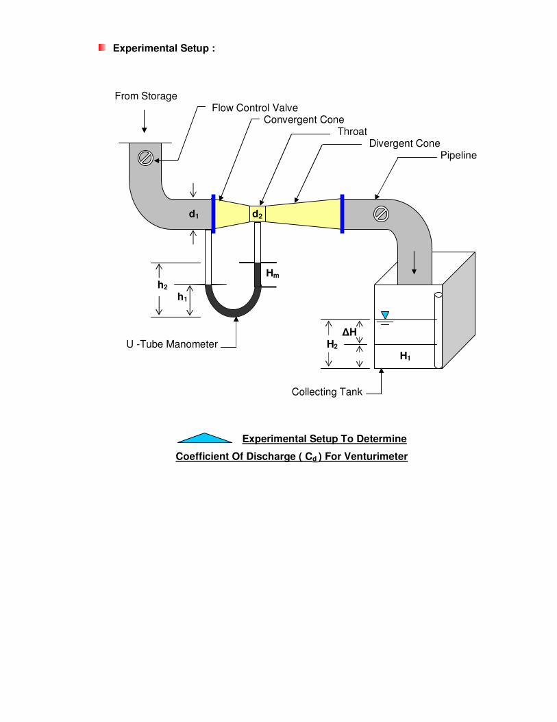
Experimental Setup : From Storage Flow Control Valve Convergent Cone Throat Divergent Cone Pipeline d1 d2 Hm h2

h1 ∆H U -Tube Manometer H2 H1

Collecting Tank

Experimental Setup To Determine

Coefficient Of Discharge ( Cd ) For Venturimeter