d OAK RIDGE NATIONAL LABORATORY

MANAGED BY MARTIN MARIETTA ENERGY SYSTEMS, INC. FOR THE UNITED STATES DEPARTMENT OF ENERGY

3 4 4 5 b 0377846 0 ORNL/TM-12660

Fluid Dynamic Demonstrations for Waste Retrieval and Treatment

E. L. Youngblood, Jr. T. D. Hylton J. B. Berry

R. L. Cummins F. R. Ruppel R. W. Hanks

This report has been reproduced directly from the best available copy.

Available to DOE and DOE contractors from the Office of Scientific and Technical Information, P.O. Box 62, Oak Ridge, TN 37831 ; prices available from (61 5) 576-8401, FTS 626-8401.

Available to the public from the National Technical Information Service, US. Department of Commerce, 5285 Port Royal Rd., Springfield, VA 22161.

This report was prepared as an account of work sponsored by an agency of the United States Government. Neither the United States Government nor any agency thereof, nor any of their employees, makes any warranty, express or implied, or assumes any legal liability or responsibility for the accuracy, completeness, or usefulness of any information, apparatus, product, or process disclosed, or represents that its use would qot infringe privately owned rights. Reference herein to any specific commercial product, process, or service by trade name, trademark, manufacturer. or otherwise, does not necessarily constitute or imply its endorsement, recommendation, or favoring by the United States Government or any agency thereof. The views and opinions of authors expressed herein do not necessarily state or reflect those of the United States Government or any agency thereof.

1

ORNL/TM- 12660 [: - 1. 1 ” .

I \ Chemical Technology Division

FLUDD DYNAMIC DEMON!TI’RAnONS FOR WASTE RETRzEvAL ANDTREATMENT

E. L. Youngblood, Jr. T. D. Hylton

J. B. Berry R. L. Cummins F. R. Ruppel’ R. W. Hankst

* Instrumentation & Controls Division t Richard W. Hanks Associates, Inc., Slurry Transport Consultant

Date Published: February 1994

NOTJCE This dowment contains information of a preliminary nature. I t is subject to revision or correction and therefore does not represent a final report.

Prepared for the OAK RIDGE NATIONAL LABORATORY

Oak Ridge, Tennessee 37831-6330 managed by

MARTIN MARIETTA ENERGY SYSTEMS, INC. for the

U.S. DEPARTMENT OF ENERGY under contract DE-AC05-840R21400

3 41tSb 0 3 7 9 8 4 6 0

LISTOFFIGURES .................................................. v

LISTOFTABLES .................................................. vi

1 . INTRODUCTXON ................................................ 2

2 . DESCRIPTION OF EQUIPMENT ..................................... 3

3 . PROCESS PARAMETERS AND PROCEDURES ....................... 6

4 . NON-NEWTONIAN MODELS AND FLOW CORRELATIONS ............ 8

4.1 Rheological Models ........................................... 8 4.2 Viscometry and Data Analysis .................................. 11

4.2.1 Experimental Data .................................... 12 4.2.2 Data Reduction and Analysis ............................ 12

4.3 Pipeline Flow Correlations .................................... 13

4.3.1 Newtonian Fluids ..................................... 13 4.3.2 Bingham Plastic fluids ................................. 14 4.3.3 Power Law Fluids .................................... 15 4.3.4 Yieid Power Law Fluids ................................ 16

4.4 IBM PC Programs ........................................... 16

4.4.1 Commercially Available Programs ......................... 17 4.4.2 Software Development Projects Required .................. 19

5 . WASTE CHARACTERIZATION AND SIMULANT DEVELOPMENT .... 21

5.1 Melton Valley Storage Tank Waste .............................. 21 5.2 Hanford Single-Shell Tanks .................................... 27

6 . SUPERNATE RHEOLOGY MEASUREMENTS ......................... 30

7 . CALIBRATION OF PIPELINE VISCOMETERS IN SLURRY 'ITST LOOP ... 30

8 . RESULTS OF RHEOLOGICAL MEASUREMENTS FOR SIMULATED W A S E ........................................... 34

8.1 Rheological Measurements for Simulated MVST Slurry ................ -34

Runs MVST 3.3A, 3B. and 3C ........................... 42

8.1.1 RunMVSTl ........................................ 38 8.1.2. Run MVST 2 ........................................ 42 8.1.3

... 111

8.2 Rheological Measurements of Simulated Hanford Single Shell Tank Waste . . . . . . . . . . . . . . . . . . . . . . . . . . . . . . . . . . . . . . . . . . . . . . . . . . . . 43

9 . PERFORMANCE OF EQUIPMENT AND INSTRUMENTATION . . . . . . . . . 49

10 . SUMMARY AND CONCLUSIONS . . . . . . . . . . . . . . . . . . . . . . . . . . . . . . . . . . 49

ACKNOWLEDGMENTS ............................................. 50

REFERENCES . . . . . . . . . . . . . . . . . . . . . . . . . . . . . . . . . . . . . . . . . . . . . . . . . . . . . 51

APPENDIXA . . . . . . . . . . . . . . . . . . . . . . . . . . . . . . . . . . . . . . . . . . . . . . . . . . . . . . . 53 APPENDIXB ........................................................ 74

iv

FIGURES

Fi-mre Page

Flow diagram of slurry test loop ....................................... 4

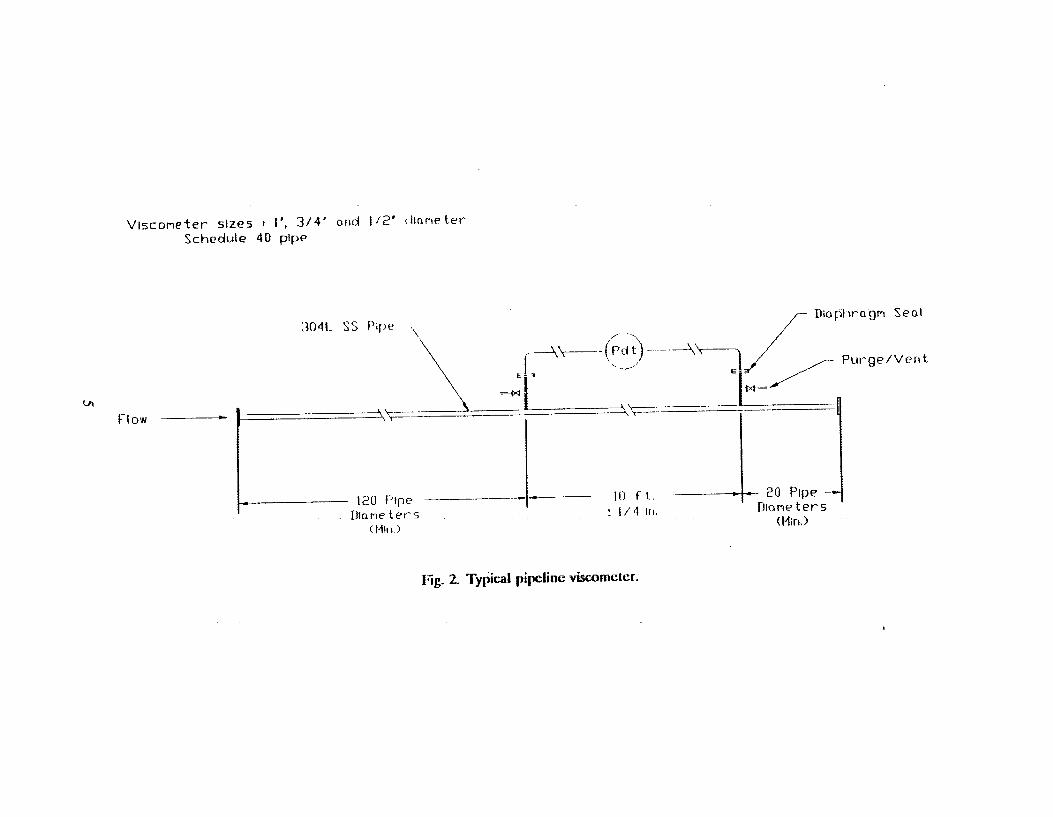
Typical pipeline viscometer .......................................... 5

1 .

2 .

3 .

4 .

5 .

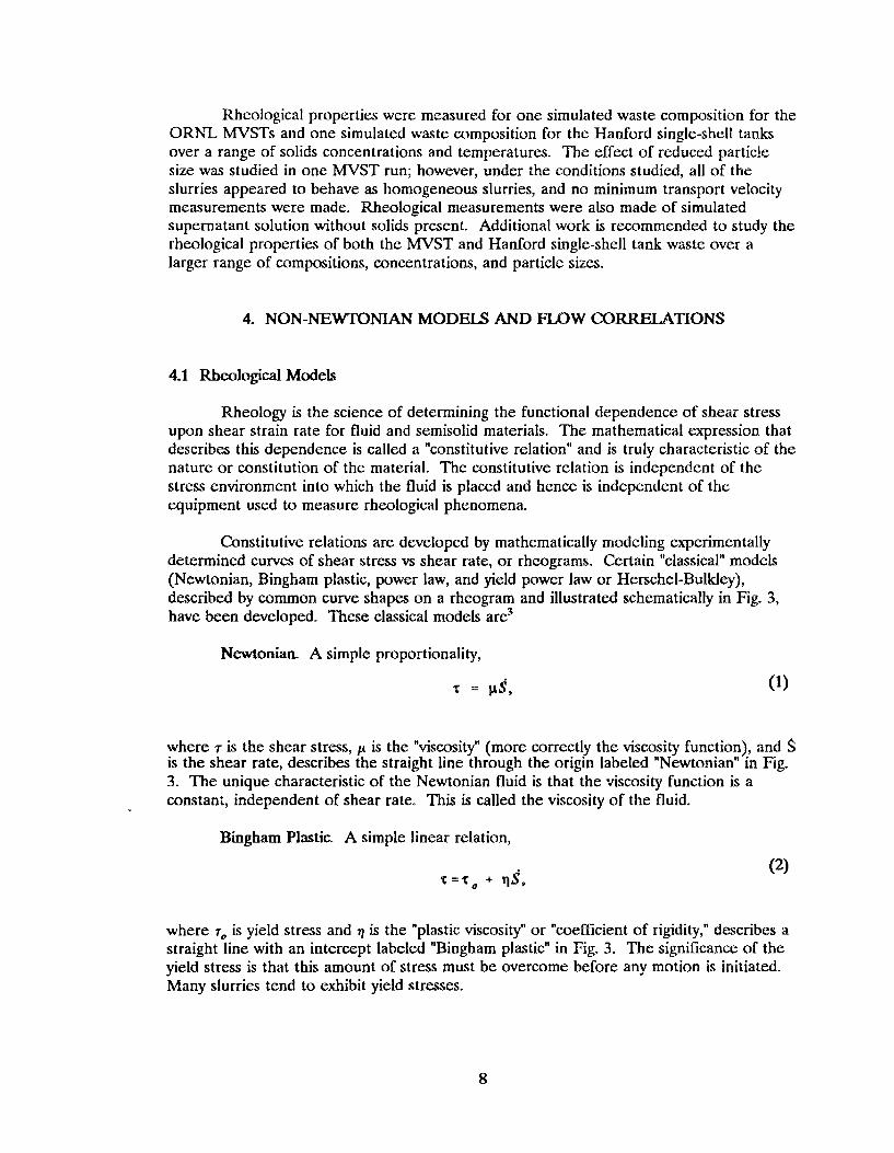
Shear stress vs shear rate curves for typical Newtonian and non-Newtonian fluids . 9

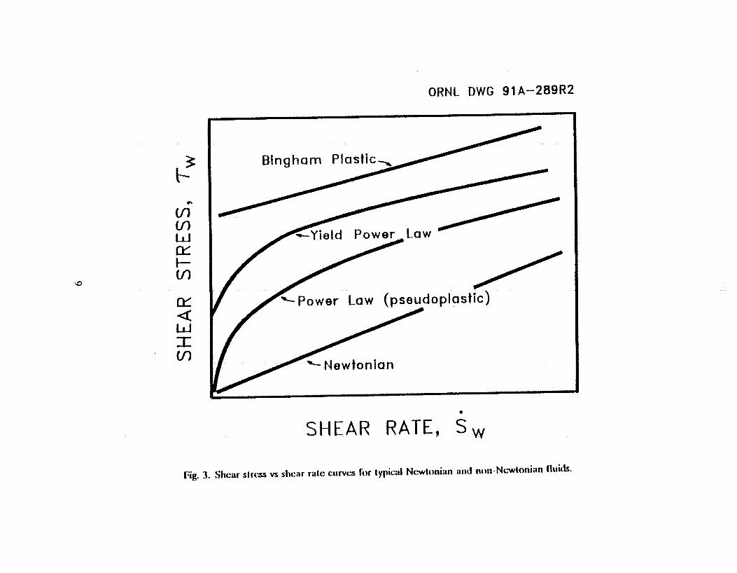
.... 29 Apparent viscosity vs shear rate for Hanford single-shell waste and simulant

Pipeline viscometer (0.18-in. ID) calibration curves ....................... 32

6 .

7 .

8 .

9 .

10 .

11 .

12 .

13 .

14 . 15 .

16 .

Rheograms for simulated Meiton Valley Storage Tank (MVST) supernate and Hanford salt cake ................................................ 32

Rheogram from calibration of pipeline viscometers with sucrose salutions ...... 35

Pipeline viscometer calibration curves with water ......................... 36

Pipeline viscometer calibration curves with 50 wt % sucrose solution .......... 36

Plot of Ap/Q versus flow rate for calibration of pipeline viscometers for 50 wt % sucrose solution ............................................ 37 Pressure drop vs flow rate for MVST 1 simulated sludge through pipeline viscometers ..................................................... 39

Flow curve for simulated MVST 1 slurry ............................... 40

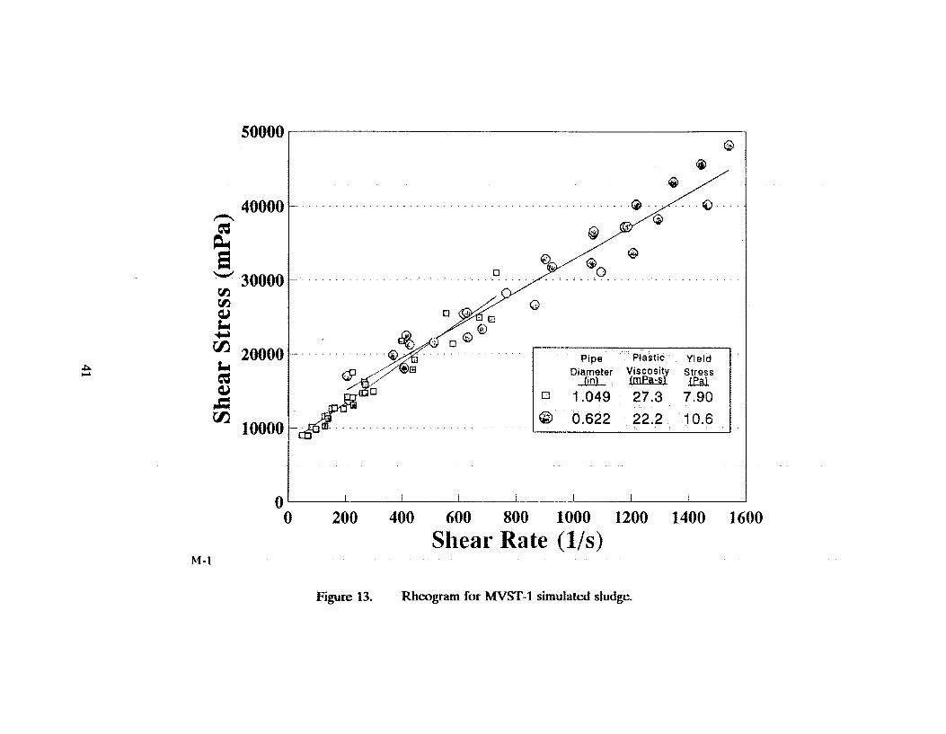
Rheogram for MVST 1 simulated slurry ................................ 41

Pressure drop vs flow rate curves for run H.2 ............................. 47

Rheograms for run H.2 ............................................. 47

Measured and calculated friction factors and critical Reynolds numbers for run H-2 ...........................................................

V

TABLES

Table

1 . Instruments and equipment used in the slurry test loop ...................... 7

2 . Range of compositions of major components and properties of Melton Valley Storage Tank waste ................................................ 22

3 . Physical properties of Melton Valley Storage Tanks W26 and W28 and evaporator waste tanks W21 and W23 . . . . . . . . . . . . . . . . . . . . . . . . . . . . . . . . . . . . . . . . . . 23

4 . Melton Valley Storage Tank surrogate composition ........................ 25

5 . Viscosity measurements for Melton Valley Storage Tank waste and simulated waste mixtures . . . . . . . . . . . . . . . . . . . . . . . . . . . . . . . . . . . . . . . . . . . . 26

6 . Composition of synthetic single-shell tank salt cake ........................ 28

7 . Composition of synthetic sludge . . . . . . . . . . . . . . . . . . . . . . . . . . . . . . . . . . . . . . 28

8 . Composition of mixtures used €or supernatant viscosity measurements . . . . . . . . . . 31

9 . Viscosity measurements for simulated supernatant liquids and calibration fluids .... - 3 3

10 . Summary of rheological measurements with Melton Valley Storage Tank simulant in the slurry test loop ........................................... 44

11 . Summary of rheological measurements with Hanford simulated waste ............. 46

vi

FLUID DYNAMIC DEMONSTRATIONS FOR WASTE RETRIEVAL, ANDTREATMENT

E L Youngblood, Jr., T. D. Hylton, J. B. Berry R L CumminS, E R Ruppel, R W. Hanks

A large quantity of radioactive waste is stored as a two-phase mixture of sludge and supernatant liquid in underground storage tanks at US. Department of Energy facilities. There is a need to transport the waste from the tanks to other locations for processing or for improved storage. One method used in the past and expected to be used in the future is transport by pipeline. Past experience has shown that the slurry behaves as a non-Newtonian fluid and that the use of correlation for Newtonian fluids for the design and operation of slurry pipelines could result in considerable error. The objective of this study was to develop or ideati9 flow correlations for predicting the flow parameters needed for the design and operation of slurry pipeline systems for transporting radioactive waste of the type stored in the Hanford single-shell tanks and the type stored at the Oak Ridge National Laboratory (ORNL). This was done by studying the flow characteristics of simulated waste with rheological properties similar to those of the actual waste.

Chemical simulants with rheological properties similar to those of the waste stored in the Hanford single-shell tanks were developed by Pacific Northwest Laboratories, and simulated waste with properties similar to those of ORNL waste was developed at ORNL for use in the tests. Rheological properties and flow characteristics of the simulatd slurry were studied in a test loop in which the slurry was circulated through three pipeline viscometers (constructed of In-, 3/4-, and i-in. schedule 40 pipe) at flow rates up to 35 gal/min. Runs were made with ORNL simulated waste at 54 wt % to 65 wt % total solids and temperatures of 25°C and 55°C. Grinding was done prior to one run to study the effect of reduced particle size. Runs were made with simulated Hanford single-shell tank waste at approximately 43 wt % total solids and at temperatures of 25°C and 50°C. The rheology of simulated Hanford and O W L waste supernatant liquid was also measured.

The results indicated that both the ORNL and Hanford wastes were non- Newtonian and could be represented by the Bingham plastic model under the conditions studied. Mathematical models and commercially available computer programs for calculating pressure drop, critical Reynolds numbers, and minimum transport velocities were identified and described by a slurry transport consultant €or the project Comparison of measured values of pressure drop and critical Reynolds numbers with calculated values using a commercially available computer program (YPLPIPE) showed good agreement. The simulated waste used behaved as a homogeneous slurry (i.e., did not settle); minimum transport velocities were not studied.

Additional studies using slurries with a wider range of composition, particle size, and suspended solids concentration are recommended. Additional work needed to develop computer programs for analysis of data from pipeline viscometers and to modify existing programs for calculating deposition velocity for nowNewtonian fluids and fluids that contain particles of more than one density is described.

1. INTRODUCIION

Waste management and environmental restoration programs have identified a need for the development, demonstration, testing, and evaluation of methods to retrieve and transport radioactive waste that is stored in underground tanks at U.S. Department of Energy (DOE) facilities. A large quantity of the waste is stored as two-phase mixtures of sludge and supernatant. The Hanford Site has 149 single-shell waste tanks with capacities up to 1 million gallons each, the Oak Ridge National Laboratory (ORNL) has eight primary waste storage tanks (50,000 gal each) filled with waste, and additional waste is stored at other DOE facilities.

One method of removal and transport of radioactive waste used in the past and planned for future use is mixing the liquid and sludge phases to produce a slurry that is transported by pipelines. Past experience has shown that the slurry behaves as a non- Newtonian fluid. The use of Newtonian correlations for the design and operation of slurry transport systems could result in considerable error in calculating design parameters and operating conditions.

The primary objective of the fluid dynamic demonstration project is to identify or develop mathematical models for predicting the flow parameters needed for the design and operation of slurry pipeline transport systems for the type of waste stored in the Hanford single-shell tanks and the ORNL Melton Valley Storage Tanks (MVSTs). The chemical composition and concentration o€ the waste contained in the tanks vary considerably. Because of the radioactive environment and limited accessibility, only small amounts of waste material are available for chemical analysis and rheological measurements on a laboratory scale. In this study, nonradioactive simulated waste with chemical and rheological properties similar to the actual waste is studied in a slurry test loop to provide engineering-scale data for the evaluation of flow correlations. Evaluation and testing of flow correlations that cover a range of waste compositions may enable predictions of the conditions €or pipeline transfer of the waste based on future laboratory rheology measurements of the actual waste.

Simulated waste compositions with rheological properties similar to those of the single-shell tanks at Hanford were developed by Pacific Northwest Laboratories (PNL). Simulants with rheological properties similar to those of the MVSTs were developed at ORNL for use in this study. Data from the operation of a slurry test loop using simulated waste were analyzed to determine the rheological properties of the slurry over a range of conditions. The rheological data were used to identify flow correlations (for pressure drop and transition from laminar to turbulent flow) needed for the design and operation of slurry transport pipelines. A slurry transport consultant (Richard W. Hanks Associates, Inc.) assisted in the analysis of the data and the evaluation of flow correlations. In addition, Dr. Hanks wrote Sect. 4 of this report, which describes non-Newtonian flow correlations and the computer programs available €or non-Newtonian flow calculations.

The project was sponsored by the DOE Office of Technology Development as a part of the Underground Storage Tank Integrated Demonstration program (TI" No, OR- 1112-02). Work done for this project includes modification of an existing slurry test loop

2

for use for the fluid dynamics tests, testing and calibration of instruments and equipment in the slurry loop, development of simulants for the Hanford single-shell tanks and the ORNL waste storage tanks, operation of the slurry test loop with the simulated wastes, and evaluation of the flow data obtained. Also as part of the project, a data base was prepared of the equipment and methods used in previous pipeline waste transfers at DOE facilities,' and an evaluation was made of instruments for measuring suspended soli& concentrations in slurries.2 This report describes the slurry test loop and the approach used for data analysis and correlation, provides information on simulant development, and gives rheological data obtained from operation of the test loop.

2 DESCRIPTLON OF EQUIPMENT

The slurry test loop was used to circulate the simulated waste slurry through pipeline viscometers to determine rheological properties and flow characteristics. A flow diagram of the system is presented in Fig. 1. Simulated waste slurry is made up in either feed tank F-100 or F-200 by mixing the chemical components with water in approximately 50-gal batches. During mixing and operation, slurry can be circulated from the bottom to the top of the feed tank with centrifugal pump 5-300 to assist the agitators in keeping the slurry in suspension. Size reduction of solid particles in the slurry can be accomplished by recirculating slurry from the feed tanks through mixedgrinder J-350. AFter the simulated waste s h m y has been prepared, it is circulated through the test loop at predetermined flow rates by progressive cavity pumps 5-110 (0 to 5 gal/min) and J-120 (4 to 35 gal/min). The flow rate is controlled by varying the pump speed. The level and density in the feed tank are measured by pressure differential instruments LT-100 and DT-100.

The slurry flow rate through the test loop is measured and recorded by flow instruments FE-125 (magnetic flowmeter) and by pumping from tank F-100 into tank F- 200, which is located on weigh table WT-205. Mass flowmeter FE-130 is used to measure the density of the slurry in the recirculating loop. The pumping rate is verified by measuring the change in weight vs time using weigh table WT-205. Ports are located at the feed tank and in circulation lines for taking samples to determining particle size and density measurements, for composition analysis, and for laboratory viscosity measurements. The viscosity of the slurry is measured at different shear rates (flow rates) using pipeline viscometers in the circulating loop. The loop has three horizontal pipeline viscometers (PLV-1, PLV-2, and PLV-3) of different diameters (1.049-, 0.824- and 0.622-in. ID. A sketch of the pipeline viscometers is shown in Fig. 2. Shear stress vs shear rate data for the fluid are determined by accurately measuring the pressure drop across a known length of pipe at known flow rates. Pressure-differential transmitters (PdT-155, PdT-165, and PdT-175) are used to measure the pressure drop across the pipeline viscometers. Iffhe pressure at the discharge of the pumps is measured using pressure gage PI-135 and pressure transmitter PT-125. The temperature of the slurry is measured by chromel- alumei thermocouples located in the feed tanks, in thermowells, and on the surface of the circulation loop. The temperature of the slurry is controlled (either heated or cooled) by use of heat exchanger HE-500 in the circulating loop.

3

N

u? w

N

I

a

4

N

cn

4

0

-w

t

5

Signals from the flow instruments (E-125 and FE-130), viscometer pressure- differential instruments (PdT-155, PdT-165, and PdT-175), weigh table WT-205, and the thermocouples are recorded by a data-logging system (386 PC with GenesisTM software and an MT-lOOOTM interface board).

In addition to using the instrumentation for process measurements, the instruments and equipment are being evaluated to determine reliability and suitability for use in radioactive waste transfer systems. A description of the major equipment items is given in Table 1.

3. PROCESS PARAMElEW AND PROCEDURES

A primary objective of the studies in the slurry test loop was to determine the flow behavior of simulated waste and to provide the rheological data required to select or develop flow correlations that can be used to predict conditions under which waste can be satisfactorily transported. Primary flow correlations needed for the design and operation of slurry transport systems are

pressure drop vs flow rate, region of transition from laminar to turbulent flow, and

0 minimum deposition velocity (minimum velocity at which a layer of sliding or stationary particles appear).

Rheological data needed for selection or development of flow correlations are obtained by circulating slurry through pipeline viscometers and other instrumentation in the sluny test loop. The following parameters are measured or determined:

0 pipeline viscometer diameter and length; sluny flow rate through viscometer; * pressure drop across viscometer;

0 slurry density, concentration, composition, and particle size; and 0 temperature.

Rheograms (shear stress vs shear rate diagrams) were prepared from pipeline viscometer data taken in laminar flow. Three sizes of pipeline viscometers are used to provide a wider range of shear rates and to permit evaluation of slippage of the slurry at the wall. Data from the rheograms were analyzed to select a rheological model representative of the slurry. Flow correlations available for determining pressure drop, critical Reynolds number, and minimum transport velocity were identified.

Mathematical models for use in the design and operation of pipeline slurry transport systems were evaluated by comparing calculated results using the models with measured values. The stability of the slurry and time-dependent properties were evaluated by observing changes in the rheological properties over a period of time,

6

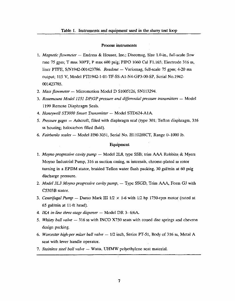
Table 1. Instruments and equipment used in the slurry test loop

procesS instruments

1. Magnetic flowmeter - Endress & Homer, Inc.; Discomag, Size 1.0-in., full-scale flow

rate 75 gpm; T max 300"F, P max 600 psig; P I P 0 1060 Cal F1.165; Electrode 316 ss,

liner PTFE, S/N1942-001423786. Readout - Variomag, full-scale 75 gpm; 4-20 ma

output; 115 V, Model FTI1942-1-01-TF-SS-Al-N4-GP3-00-SP, Serial No.1942-

001423785.

2. Mass flowmeter - Micromotion Model D 51005126, SNl13294.

3. Rosemount Model 11.51 DPfGP pressure and differential pressure transmitters - Model

1199 Remote Diaphragm Seals.

4. HoneyweIl ST3000 Smart Transmitter - Model STD624-Alk

5. Pressure gages - Ashcroft, filled with diaphragm seal (type 301; Teflon diaphragm, 316

ss housing; halocarbon filled fluid).

6. Fairbanks scales - Model H90-3051, Serial No. H110288CT, Range 0-10oO Ib.

Equipment

1. Moyno progressive cavity pump - Model 2L8, type SSB; trim AAA Robbins & Myers

Moyno Industrial Pump, 316 ss suction casing, ss internals, chrome-plated ss rotor

turning in a EPDM stator, braided Teflon water flush packing, 30 gaVmin at 60 psig

discharge pressure.

2. Model 3L3 Moyno progressive cavity pump, - Type SSGD, Trim AAA, Form G?I with

C5303B stator.

3. Centrifugal Pump - Durco Mark 111 ll2 x 1-6 with 1R hp 1750-rpm motor (rated at

65 gaVrnin at 11-Et head).

4. IKA in-line three-stage disperser - Model DR 3- 6 / 6 k

5. whitey ball valve - 316 ss with INCO X750 seats with coned disc springs and chevron

design packing.

6. Worcester high-per mizer ball valve - 1/2 inch, Series PT-51, Body of 316 ss, Metal A

seat with lever handle operator.

7. Stainless steel ball valve - Watts, UHMW polyethylene seat material.

7

Rheological properties were measured for one simulated waste composition for the ORNL MVSTs and one simulated waste composition for the Hanford single-shell tanks over a range of solids concentrations and temperatures. The effect of reduced particle size was studied in one MVST run; however, under the conditions studied, all of the slurries appeared to behave as homogeneous slurries, and no minimum transport velocity measurements were made. Rheological measurements were also made of simulated supernatant solution without solids present. Additional work is recommended to study the rheological properties of both the MVST and Hanford single-shell tank waste over a larger range of compositions, concentrations, and particle sizes.

4. N O N - ~ ~ N I A N MODELS AND FLOW CORRELATIONS

4.1 Rheological Models

Rheology is the science of determining the functional dependence of shear stress upon shear strain rate for fluid and semisolid materials. The mathematical expression that describes this dependence is called a "constitutive relation" and is truly characteristic of the nature o r constitution of the material. The constitutive relation is independent of the stress environment into which the fluid is placed and hence is independent of the equipment used to measure rheological phenomena.

Constitutive relations are developed by mathematically modeling experimentally determined curves of shear stress vs shear rate, or rheograms. Certain "classical" models (Newtonian, Bingham plastic, power law, and yield power law or Herschel-Bulkley), described by common curve shapes on a rheogram and illustrated schematically in Fig. 3, have been developed. These classical models are3

Newtonian A simple proportionality,

r = pS, (19

where 7 is the shear stress, p is the "viscosity" (more correctly the viscosity function), and s is the shear rate, describes the straight line through the origin labeled "Newtonian" in Fig. 3. The unique characteristic of the Newtonian fluid is that the viscosity function is a constant, independent of shear rate. This is called the viscosity of the fluid.

Bingham Plastic A simple linear relation,

T = r , + 51.9, (29

where 70 is yield stress and 7 is the "plastic viscosity" or "coefficient of rigidity," describes a straight line with an intercept labeled "Bingham plastic" in Fig. 3. The significance of the yield stress is that this amount of stress must be overcome before any motion is initiated. Many slurries tend to exhibit yield stresses.

8

ML

'SS

3tllS

tlV

3HS

9

If Eq. (2) is rearranged into the form of Eq. (l), the viscosity function (which is no longer a constant as in the Newtonian fluid case) is given by

To p=,+q. S

(3)

The characteristic of this variable viscosity fluid is that its viscosity function approaches infinity as shear rate becomes very small (corresponding to the presence of a finite yield stress). It also approaches r] in the limit of large shear rate. Thus, 9 is also called the "high shear limiting viscosity."

Power Law. If the Fig. 3 rheogram were replotted on logarithmic coordinates, one would see that many shear-thinning fluids (fluids whose viscosity function decreases with increasing shear rate) exhibit curves with substantial portions that are linear corresponding to

log(r) = log(K) + nlog(S). (4)

T h i s logarithmically linear equation when translated to the linear coordinates of the rheogram becomes

r=k=Sn,

which i s the well-known Power Law relation. The parameter K is called the "consistency factor," and the parameter n is called the "flow behavior index." The viscosity function for the Power h w model is

*(n-l) p = K s .

If n < 1, this viscosity function decreases with increasing shear rate, and the fluid is said to be "pseudoplastic." If n > 1, this viscosity function increases with increasing shear rate, and the fluid is said to be "dilatant" or shear thickening. In the special case where n = 1, the viscosity function reduces to the constant value K, which is equivalent to the viscosity of a Newtonian fluid. This role of the parameter n gives rise to its name of flow behavior index.

Note that for pseudoplastic fluids, Eq. (6) has a limiting value of zero as shear rate increases indefinitely. This is clearly not physically realistic as all real materials have some residual limiting high shear-rate viscosity. For this reason, the Power Law can safely be used only for interpolation between existing measured values of shear rate but not for extrapolation to higher values. The Power Law has become popular because of its mathematical simplicity.

10

Yield Power Law. If one adds a yield stress to Eq. (5), obtaining

T = 5 , + b",

one characterizes a curve similar to that labeled "yield power law" in Fig. 3, which is a Power Law model with a yield stress. The viscosity function for this model is given by

Note that for the special case n > 1, this viscosity function is shear thinning for small values of shear rate but shear thickening for large values of shear rate: that is, the viscosity of such a material first decreases, reaches a minimum value, and then increases as shear rate increases. This very complex behavior is often exhibited by high-concentration slurries of finely divided solids.

The rheological constitutive behavior of a great many slurries is almost always described by one of the above models.

4 2 V i m e t r y and Data Analysis

Viscometers are mechanical devices that create stress fields in fluid samples. They are always instrumented to measure two macroparameters, one functionally related to (but not equal to) the shear stress, and the other functionally reiated to (but not equal to) the shear rate. Thus, raw viscometer data, regardless of the type or make of the device used for their collection, must be converted into shear stress and shear rate values before any meaningful evaluation of the constitutive behavior of the fluid can be made. In the case of Newtonian fluids, this is a simple matter of multiplying each measured variable by an appropriate instrument constant. This is a direct consequence of the mathematical form of Eq. (1). For all other constitutive relations, however, this simple conversion is not possible; a more complex type of data reduction must be employed.

If one knew the correct constitutive relation for the fluid being tested, one could solve the basic differential field equations for momentum transport in the geometrical configuration corresponding to the viscometer used and obtain the functional relation between the measured variables appropriate to that constitutive relation. However, the very purpose for constructing and using a viscometer is to discover the constitutive relation of the fluid. Hence, one cannot resort to the direct comparison of data with theoretical solutions as described above. An alternative procedure is needed. For the tube or capillary or pipeline viscometer, this alternative is the method of Rabinowitsch and M ~ o n e y . ~ . ~

11

4.21 Ekperimental Data

In a pipeline viscometer, the primary measured variables are the pipe diameter, D; the length between two pressure taps, L; the pressure differential across that length, Ap; and the volume rate of flow of fluid through the pipe, Q (alternatively, one may measure the mass flow rate, rn, and the fluid density, p, from which Q may be calculated as rnlp).

4.22 Data Reduction and Analysis

For all fluids, regardless of constitutive relation, it can be very simply shown that the shear stress at the wall of the tube or pipe is related to measured variables by

A second variable, related to Q and called a "pseudo-shear rate," is

32Q - 8V r E - - - . XD' D

In the method of Rabinowitsch and Mooney, a logarithmic plot of the calculated variables 7w and r is prepared. The raw data are then smoothed by fitting a curve to then. This curve is then graphically (or numerically if computer fitting is used) differentiated at points corresponding to each experimental value of I?. The derivative thus obtained is

d l n r ,

d l n r / n =

It can easily be mathematically proved that, independent of the constitutive relation of the fluid, the shear rate at the wall may be calculated from I' by

3n' + I. 4n'

s, = r

Thus, by using the procedure outlined above, the measured variables B, L, Ap, and Q may be converted into the required rheogram variables 7w and S,. Once these variables have been calculated, a rheogram is prepared, and one of the constitutive relations is curve fitted to the data to obtain the equation parameters.

12

43 Pipeline Flow Correlations

Once the appropriate constitutive relation is known, one can determine the proper relation between Ap and Q for laminar, transitional, and turbulent flow in a pipeline. It is also possible to determine the conditions for transition from laminar to turbulent flow and for the deposition of heterogeneously suspended solids from turbulent flows as well as the Q-Ap relation for heterogeneously suspended solids in turbulent flow. There are nl:, generically applicable relations for these flow conditions, and separate results are required for each constitutive relation. We give below a brief summary of the appropriate relations for each of the constitutive relations described above, which are useful for most slurries.

43.1 Newtonian Fluids

Friction factors for Newtonian fluids are given by the well-known Moody chart. In laminar flow, the familiar result

f = - 16 av,

where

is the Fanning friction factor, and

is the Reynolds number. The above are the dimensionless equivalent of the Poiseuille equation

Transition Erom laminar to turbulent flow is determined by the condition NRc = 2100. The turbulent flow relation is given graphically by the Moody chart or numerically by a number of empirical curve-fit correlations. One that is useful for the computer is the Colebrook relation6

4f = Q + b N z

13

with k = dD being the relative pipe-wall roughness and

u = 0.094kom + 0.53k ,

b = 88k0" ,

and

c = 1.62k0-'M .

The prediction of V,, the velocity of deposition of heterogeneously suspended solids from a turbulent flow, is best accomplished by using the model of Hanks and Sloan.' This model is mathematically complex; its details are not included here. However, an IBM PC-compatible program is commercially available that permits calculation of V, using this method.

The calculation of the Q-Ap relation for heterogeneous turbulent transport of solids is accomplished by the method of Wasp.' This method has been used successfully in numerous commercial pipeline designs. An IBM PC program is commercially available that performs the necessary calculations using this method.

4 3 2 Bingham Plastic Fluids

The Bingham plastic equivalent of the Poiseuille relation for laminar flow is the Buckingham equation3

Note that even though the Bingham plastic constitutive relation is linear, this flow equation is nonlinear. It is generally true €or non-Newtonian fluid models that the integration of the constitutive relation for pipe flow produces a nonlinear flow relation.

The condition of transition from laminar to turbulent flow may be determined by using the method of Hanks.' This is mathematically complex, and the equations are not presented here. However, IBM PC programs are commercially available that make this calculation.

Friction factors for the turbulent flow of Bingham plastic fluids must be calculated by the method of Hanks and Dadia." IBM PC programs for using this method are also commercially available.

14

In some of the early studies of turbulent flow of Bingham plastic fluids, it was erroneously concluded" that one could use the conventional Moody diagram of Newtonian flow with p re laced by 7 in the Reynolds number to calculate friction factors if 7* c 24 N/m2 (240 d/cm ). While there are some combinations of flow and rheological parameters for which this procedure fortuitously works, there are also many combinations of flow and rheological parameters for which this procedure will produce significantly erroneous results. Therefore, only the method of Hanks and Dadia should be used.

5

No direct computational model is available for predicting V,, for non-Newtonian fluids of any type. The method of Hanks and Sloan could be modified to include non- Newtonian constitutive relations, but this would require a special development effort. This same situation exists for the calculations of the Q-& relation for solids suspended heterogeneously in non-Newtonian fluids.

A combination experimental-computational method modifying Wasp's method has been developed by Hanks for calculating heterogeneous turbulent head losses in non- Newtonian fluids.I2 However, this method invokes extensive, detailed experimental evaluation of the dependence of constitutive model parameters on both solid concentration and particle-size distribution.

433 Power Law Fluids

For the power law constitutive relation, the equivalent of the Poiseuille equation for laminar flow is

This equation can be expressed in dimensionless form identical to the Newtonian result as

f=- 16 *am

where N',pL is a power law "Reynolds number" defined by

Because of the simple: form of the power law model and the form of Eq. (23), Metzner and Reed sought to develop a generalized method of data representation that would make Eq. (23) applicable for all fluids.I3 They succeeded in manipulating the method of Rabinowitsch and Mooney, described earlier, into the form

15

f=- 16 &P?MR

where NkNR is a "generalized" Reynolds number defined by

with n' being the Rabinowitsch-Mooney parameter defined earlier and K' being the intercept value of the straight line of slope n' tangent to the curve of log rW vs log(8YD) at the point where n' is determined. In the special case where the Rabinowitsch-Mooney plot is a straight line (i.e, the fluid is truly a power law in the range of the data), we have n = n' and K' = K so that Eqs. (24) and (26) reduce to the identity NmFL = NmHF

Because of the generality of the Rabinow'tsch-Mooney relation in laminar flow, h s . (25) and (26) correlate laminar flow data for any fluid, regardless of its true constitutive relation. This generality was erroneously assumed to extend to transitional and turbulent flow.13 Thus, Metzner and Reed proposed that Newtonian turbulent flow correlations could be used to predict non-Newtonian flow behavior if Nm were replaced by NRefifR Unfortunately, this is not true; more complex results are required. Hanks has shown that since the Rabinowitsch-Mooney relation is not valid in turbulent flow, it is impossible to correlate turbulent flow data using NmMF Rather, one must develop separate models for each constitutive relation.

The prediction of conditions of transition from laminar to turbulent flow for power law fluids may be accomplished by using the method of Ryan and Johnson" or Hanks.I6 The prediction of turbulent-flow friction factors may be accomplished by using the method of Hanks and Ricks.I7 An IBM PC program to accomplish these calculations is commercially available.

43.4 Yield Power Law Fluids

Because of the presence of a third parameter in the yield power law constitutive relation, the mathematical expressions for laminar and turbulent flow Q-Ap relations and the conditions for transition from laminar to turbulent flow are quite complicated and are not presented here. However, they are commercially available for performing calculations for all three conditions.

and IBM PC programs are

4.4 IBM PC Programs

Mention was made several times of commercially available IBM PC programs to perform the various model calculations described. Here is a brief overview of what these programs contain and how they work. All the programs described below are available

16

from Richard W. Hanks Associates, Inc. They were developed and written by Dr. Hanks, the slurry consultant on this project.

Also presented is an outline of the development efforts that will be required to create currently unavailable programs needed to successfully carry out all of the studies proposed in this project.

4.4.1 Commercially Available Programs

4-4.1.1 YPLPIPE

The program code named YPLPIPE is an interactive, menu-driven program that allows the operator to select a variety of different calculations, Based upon the turbulent pipe-flow model of Hanks" for Yield Eower h w PTF'Eflow, it allows the operator bo input values of T,, K , n, and p, together with various combinations of D, Q, or -4. The last three are entered in pairs, and the third variable is calculated. If r0 = 0 is entered, the model of Hanks and Ricks17 is used to compute power law behavior. If n = 1, K = 71 is entered, the model of Hanks and Dadia" is used to compute Bingham piastic behavior. If T~ = 0, K = p, and n = 1 is entered, the Newtonian flow models are used.

Thus, this one program handles all four rheological constitutive models with equal ease. In addition to the computation of either laminar or turbulent friction factors, pressure losses, or flows, this program also computes all pertinent variables corresponding to the transition from laminar to turbulent flow for any of the four constitutive models.

In addition to the above features, the program also permits the operator to select from any of the commonly used systems of units for each of the appropriate input variables and output results. All unit conversions are automatically handled internal to the program. The selections of units, types of variables to be input o r output, whether laminar or turbulent flow is desired, and whether a single point or an entire friction factor curve is desired are all made by simple menu-selection key strokes.

For laminar flow calculations, the appropriate equivalent of the Poiseuille equation (listed above for the various models) is solved to give Q(D, -@/I,), -4p/L(Q,D), or D(Q, -bp/L), depending on the choice of input variables selected. For the transition from laminar to tutbufent flow, the various equations that have been developed €or the four models are solved. Some of these are direct calculations while others require iterative computation.

The turbulent flow calculations all require evaluation of systems of equations from the various models. All of these involve the numerical evaluation of complicated integrals. This is accomplished by means of a 20-point Gaussian quadrature routine that is extremely accurate. All calculations require iterative solution of one o r more equations that in most cases are coupled. The iterations use cornbinations of Newton's method and quadratic interpolation for root-finding. These iterative methods converge quite rapidly and are very stable numerically.

17

4.4.12 SLOANVDC

A program code named SLOANVDC uses the method of Hanks and Sloan to compute V, for heterogeneously suspended solids in Newtonian liquids. The program allows the operator to input complete particle-size distribution (PSD) data, particle and fluid densities, fluid viscosity, pipe diameter, and solids concentration. The program also can accommodate the situation where the solid absorbs a certain percentage of the liquid (the inherent moisture problem).

In this model, two coupled, nonlinear differential equations must be solved simultaneously. This is performed in an iterative fashion with all integrations made by the same 20-point Gaussian quadrature routine used in WLPIPE.

The PSD data are analyzed to determine a portion that is presumed to be uniformly and homogeneously suspended. This portion of the PSD, together with the suspending liquid, is treated as a single-phase, Newtonian fluid called the "vehicle." A density and viscosity are computed for the vehicle using well-known correlations. The remainder of the particles are presumed to be heterogeneously suspended in this vehicle. The heterogeneously suspended portion of the PSD is then analyzed to determine for it a value of d,, (the diameter for which 85% of the particles are smaller). In the model, all particles are treated as if they were uniform spheres of this diameter. The value of V, computed by this program is the sliding-bed deposition velocity (the minimum velocity at which a layer of sliding particles appears) for spheres of diameter d, heterogeneously suspended in the vehicle in the pipe of diameter D (which was input).

4.4.13 WASP

A program code WASP solves the model equations of Wasp to calculate the head loss (either single velocity value or complete velocity curve between input limits) for heterogeneously suspended particles in a Newtonian fluid. The program permits the operator to input a complete PSD, pipe diameter, solid and fluid densities, fluid viscosity, particle fluid absorbtivity, and operating velocity or a range of velocities if a full C U N ~ is desired.

In the method of Wasp, a portion of the solids is presumed to be uniformly and homogeneously suspended in the liquid, creating a Newtonian "vehicle" (like in SLOANVDC). The remainder of the solid particles are presumed to be heterogeneously suspended in this vehicle and to obey Durand's correlat i~n. '~

The vehicle is determined by an iterative process in which a fraction is assumed, density and viscosity are calculated, and a concentration distribution is calculated from a model chosen by Wasp. When the fraction determined from the calculated concentration distribution equals the assumed fraction, the iteration is converged. This process usually converges quite rapidly. The remainder of the particles are then assumed to be heterogeneously suspended. All iterations are converged to four digits of agreement.

18

4.4.1.4 LO0PFLx)W

An IBM PC program LOOPFLOW is available that permits analysis of durrry pressure-drop data obtained in a recirculating flow loop. The extremely useful feature of this program is its ability to analyze time-dependent changes in slurry properties caused by particle attrition. This phenomenon can be very important if particles break up either due to physical fracturing or chemical dissolution (a distinct possibility with the slurry systems to be studied in the present projects). When particle attrition or chemical dissolution occurs, the Q-Ap relation observed in a recirculating flow loop is not the same as would be observed in a single-pass-through pumping system. Consequently, the data are not useful unless the effect of the time-dependent properties can be correctly accounted for. LOOPFLOW is capable of doing this. Details of the program and its computational methods are very complicated and extensive and will not be presented here.

4.42 Software Development Projects Required

4.421 Viscometer Data Reduction and Analysis

The only proper method of viscometer data reduction is the method of Rabinowitsch and Mooney described above. However, this method is very laborious and slow when performed graphically by hand. Therefore, it is important that a user-friendly, menu-driven, interactive IBM PC graphics program be developed that can accomplish this method quickly. This same program should also have the capability of curve-fitting any of the four rheological constitutive modek to the derived rheograms and determining appropriate model parameters.

Several years ago, Dr. Hanks developed a program for Battelle PNL to perform similar types of operations €or data obtained with their Haake rotational viscometer.m Because of the fundamental differences between the rotational viscometer and the pipeline viscometer used by ORNL, the details of the data-reduction and computational models used are quite different, and the PML programs cannot be used for the ORNL data. However, many of the basic data-handling procedures, curve-fitting procedures, and graphics display methods used in the PNL programs can be readily adapted to the Rabinowitsch-Mooney procedure required for the ORNL data.

As a part of the ongoing work of this project, Dr. Hanks will develop a menu- driven program similar to the PNL program but adapted to the ORNL needs. ne program will permit input of raw data from the ORNL data-collection system and will convert the raw data to T~ and 8V/D equivalents. The program will use the smoothed Rabinowitsch-Mooney curves in the calculation of n' values and reduction of 8V/D values to equivalent shear rate values to create the rheogram. Once the rheogram is calculated, the program will use nonlinear regression and interactive parameter variation methods, together with graphics display of the data, fitted curves, and distributions oE deviations between data and calculated values to allow the operator to curve fit any of the four constitutive models to the rheogram data. Finally, it will output raw data, converted data, rheogram data, and model parameters in any set of units desired. All internal calculations will be performed using SI units as the standard. All unit conversions will be handled internally in the program. No hand computations or graphical procedures will be required.

19

4.4.2.2 €&tension of SLQANVDC to Include Non-Newtonian Constitutive Relations

At present, SLOANVDC is restricted to Newtonian fluid behavior. While it is possible to extend this model to include various non-Newtonian constitutive models, this extension is not trivial because it requires the separate solution of the calculation of particle concentration distributions in the non-Newtonian fluid. In the case of the yield power law model, and perhaps also the power law model, this may require simultaneous numerical integration of coupled differential equations because of the nonlinearity of the fundamental constitutive relations.

As a part of the ongoing work of this project, Dr. Hanks will develop the appropriate mathematical solutions and computer programs to perform this extension. This extension is very important because the presence of a yield stress (as in both the Bingham plastic and yield power law models) will greatly influence the suspending power of the fluid in the slurry.

The computer program to be developed will be patterned rather closely after the present SLOANVDC with the addition of menu selections for choice of constitutive model to be used. It will be written in the following two versions: a a stand-alone version that may be used to compute Voc for given input conditions, and e a subroutine version that may be coupled with other programs that may require V,, as

part of a more extensive computation.

4-4-23 Extension of WASP to Include Multicomponent Mixtures of Solids Having More Than One Density and Non-Newtonian Vehicle Rheology

All of the simulant slurries to be studied in this project will be composed of multicomponent mixtures of different materials. The real slurries at Hanford and other sites also contain numerous materials. Any slurrying process used in the real system will undoubtedly create a slurry with a number of different-density heterogeneously suspended solids. I t is also quite likely that the real slurries will have non-Newtonian rheological behavior under some conditions. The current versions of WASP are based upon Wasp's original model,' which presumed that only a single-density solid was present and that the vehicle portion of the mixture behaved as a Newtonian fluid.

As part of the ongoing work of this project, Dr. Hanks will develop the necessary mathematical and computer models to extend the current method of Wasp to include a multicomponent mixture of solids of differing densities. Each different-density solid will be presumed to have its own PSD to permit complete flexibility in specification of slurry properties. Two versions of the method will be developed:

e a program presuming the vehicle to be Newtonian, and e a more expanded version presuming the vehicle to be non-Newtonian with choice of

consti tu tive relations.

The second version will require the inclusion as a subroutine of the upgraded non- Newtonian version of SLOANVDC as well as models for concentration dependence of constitutive relation parameters.

5. WA!XJ3 CXARA-nON AND S I M U L A N T DEVELOPMENT

Because of the difficulty in working with radioactive waste, nonradioactive simulants that have rheological and physical properties (Viscosity, density, and particle size) similar to those of samples taken of actual waste were used for the fluid dynamics tests in the slurry test loop. Because rheological properties of many of the waste tanks have not been measured, it is desirable to have simulants based on formulations that can be extrapolated to simulate the properties of the wide ranging waste compositions contained in the Hanford and ORNL tanks. This can best be accomplished by the use of simulants with chemical compositions similar to those of the actual waste, although the mechanism by which the chemical compounds were formed in the waste tanks and changes that result from exposure to heat and radiation cannot be duplicated.

5.1 Melton Valley Storage Tank Waste

MVSTs contain a two-phase waste material. The supernatant is an aqueous solution composed primarily of sodium and potassium nitrate; the major radionuclides present are strontium and cesium?’ There is a 2- to 5-ft-deep sludge accumulation on the bottom of the tanks, composed primarily of particles of calcium and magnesium hydroxides and carbonates with smaller amounts of aluminum and iron compounds. Sodium and potassium nitrate are present as dissolved salts in the interstitial area between particles. The sludge also contains uranium, thorium, radionuclides, and transuranic elements. Settling tests indicate that the sludge particles have an agglomerate radius of about 20 pm.” The consistency of the sludge in the tanks ranges from soft sludge to hard mud.

The method proposed for removal and disposal of the waste in the MVST is by sluicing with supernatant and transporting by pipeline to a proposed Waste Handling and Packaging Plant where the material will be solidified, packaged, and sent to the Waste Isolation Pilot Plant in Carbbad, New Mexico, for disposal.23 A similar method of mobilization and transport was used to transfer slurry From the ORNL Gunite tanks to the MVSTs in 1983.”

Analytical measurements have not been made to identify the specific chemical compounds (only anion and cation species) present in the MVSTs. The simulated waste composition for the MVST is based on the cation and anion analysis of the sludge and supernatant liquid. A chemical simulant composition was initially formulated by hrlattusZ based on the composition of MVST waste tanks W26 and W28. The simulant composition was modified for this study to include sample information taken from other tanks and chemically characterized by Sears et aL2’ from samples taken between September 19 and December 5, 1989, and physical characterization of the sludge samples by Ceo et a].= Major components in the sludge and supernatant liquid phases are summarized in Table 2, and the physical properties of selected waste tank samples are given in Table 3.

21

Table 2 Range of compositions of major component and properties of Melton Valley Storage Tanks waste

Supernatant liquid

Dissolved solids content: 334 g/L to 478 g/L

Density: 1.21 g/mL to 1.28 g/mL

pH range: 11 to 13

Nitrate concentration: 3 M to 5 M with average of 4 M

Sodium concentration: 61 g/L to I10 g/L

Potassium concentration: 8 g/L to 78 g/L

Potassium/sodium mass ratio: 0.1:0.3, except tanks W26 and W23 at 0.8:l.O

Chloride concentration: about 0.08 M

Sludge phase

Total solids (dissolved plus undissolved): 400 to 500 gkg

Density: 1.3 to 1.5 $/mL

Sodium plus potassium Concentration: 40 to 60 wt % of the total metal concentration

Calcium plus magnesium concentration: 30 to 40 wt % of the total metal concentration

Uranium plus thorium concentration: 4 to 20 wt % of the total metal concentration

Aluminum concentration: 0.1 to 0.8 wt % of total metal concentration

Iron concentration: 0.1 to 0.25 wt % of total metal concentration

*Includes some of the evaporator facility waste tanks. Source: M. B. Sears, et ai., SampIing and Analysis of Radioactive Liquid and Waste Sludges in the Melton Valley and Evaporator Faciiify Storage Tanks at O W L , ORNLflM-11652, Oak Ridge National Laboratory, Oak Ridge, Tenn., September 1990.

22

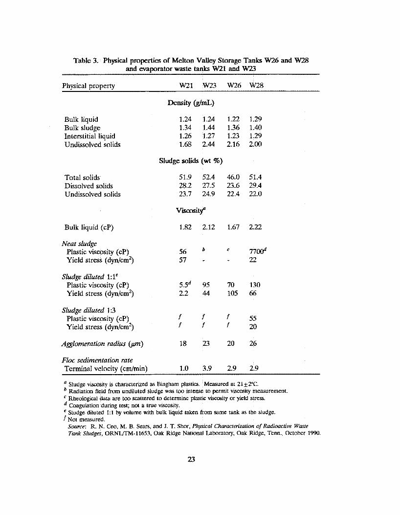
Table 3. Physical properties of Melton Valley Storage Tanks W26 and W28 and evaporator waste tanks W21 and W23

Phvsical DroDertv W21 W23 W26 W28

Buik liquid Bulk sludge Interstitial liquid Undissolved solids

Total solids Dissolved solids Undissolved solids

Bulk liquid (cP)

Neat sludge Plastic viscosity (cP) Yield stress (dyn/cm2)

Sludge diluied l:le Plastic viscosity (cP) Yield stress (dyn/cm2)

Sludge diluted 1:3 Plastic viscosity (cP) Yield stress (dyn/cm2)

1.24 1.24 1.22 1.29 1.34 1.44 1.36 1.40 1.26 1.27 1.23 1.29 1-68 2.44 2.16 2.00

Sludge solids (wt %)

51.9 52.4 46.0 51.4 28.2 27.5 23.6 29.4 23.7 24.9 22.4 22.0

Viscosi?$

1.82 2.12 1.67 2.22

C 7 7 d 56 57 - 22

5.5d 95 70 130 2.2 44 105 66

f f f 55 f f f 20

Agqlomeration radius (p) 18 23 20 26

Floc sedimentation rate Terminal velocity (cm/min) 1.0 3.9 2.9 2.9

SIudge viscosity is characterized as Bingham plastics. Measured at 21 f2”C. Radiation field from undiluted sludge was too intense to permit viscosity measurement. Rheological data are too scattered to determine plastic viscoSity or yield stress. Coagulation during test; not a true wcosity. Sludge diluted 1:l by volume with bulk liquid taken from same tank as the sludge.

Source: R. N. Ceo, M. €3. Sears, and J. T. Shor, Physical Characieriration of Radioactive Waste Tank Sludges, OR--11653, Oak Ridge National Laboratory, Oak Ridge, Tenn., October 1%.

f Not measured.

23

Viscosity measurements for the MVST sludge were limited to relatively low shear rates (16 s-l) by the radioactive sample size that could be handled and the viscometer used. Measurements at higher shear rates that are closer to the operating shear rates (on the order of 500 s-*) are needed for accurate modeling. Also, no information is available on whether the viscosity of the slurry is time dependent.

The simulant developed for the MVSTs was based on the major chemical components in the waste given in Table 2. The composition of the initial soluble and insoluble components of the simulated sludge is given in Table 4. Other mixtures were made by adding higher concentrations of insoluble components in the same proportions as given in Table 4. The simulant was made by mixing bulk chemicals as purchased from the manufacturer. Laboratory viscosity measurements were made using a Fann Model 35A viscometer for comparison with viscometer data from the actual waste to determine the composition ranges for use in the slurry test loop. The results, shown in Table 5, indicate that the simulant has a yield stress and exhibits a non-Newtonian behavior that can be represented as a Bingham plastic (as does the actual waste). However, the simulated waste composition required a considerably higher total solids concentration to achieve yield stresses and plastic viscosities similar to those of the actual waste. The sludges from the different tanks have considerably different plastic viscosities for similar solids concentrations. The rheological properties of the simulant are in the same general range as expected for the actual waste after dilution for mobilization.

The particle size of the simulated waste is somewhat similar to that of the actual waste; however, the same methods of size determination were not used. As shown in Table 3, the agglomeration radius of the sludge from four of the waste tanks is in the range of 20 prn. Particle size measurements were made for the simulant mixture given in Table 4 using a k e d s and Northrup Microtrac laser scanner and by optical image analysis. Results from the Microtrac indicate that 99 wt % of the particles are less than 30 pm in diameter and have a volume mean diameter of 10 pm. Results from image analysis indicate. that the particles have a maximum and minimum area equivalent diameter of 22.06 and 0.58 pm and an average area equivalent diameter of 1.82 pm.

To determine the effect of grinding and particle size reduction on the rheology of the sludge, the simulant composition given in Table 4 was homogenized for 1 h with an IKA Labortechnik Ultra-Turrax 125 homogenizer. Grinding resulted in an obvious change in the appearance and settling rate of the sludge. Optical image analysis indicated a reduction in the maximum particle diameter from 22.06 pm to 10.94 pm and a reduction in the average diameter from 1.82 pm to 1.23 pm- A slight increase in particle size (a mean volume diameter increase from 10 pm to 11 pm) was indicated by the Microtrac measurement. As shown in Table 5, grinding of the simulant resulted in an increase of the yield stress from 20 dyn/cm2 to 36 dyn/cm2; however, the plastic viscosity remained essentially the same at about 4 CP to 5 cP.

The sirnulant composition discussed above was considered acceptable for the initial studies in the slurry test loop; however, additional work is recommended to identify other factors that may be important in determining the properties of the sludge.

24

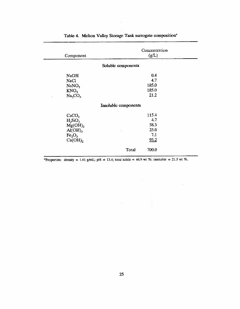
Table 4. Melton Valley Storage Tank surrogate composition"

Concentration Component

Soluble components

NaOH NaCl NaNO, mo3 Na2C0,

0.4 4.7

185.0 185.0 21.2

Insoluble components

115.4 4.7 58.3 25.0 7.1 - 93.2

Total 700.0

"Properties: density = 1.41 ghnL; pH = 13.4; total solids = 46.9 wt %; insoluble = 21.5 wt %.

25

Table 5. Vmmsity measurements for Melton Valley Storage Tax& waste and simulated waste mixtures

Total solids Insoluble' Plastic viscosity Yield stress (wt "/.I (wt %'.> (CP> ( dyn/cm2)

Simulated wasteb

46.9 21.5 4 20

46.9

62.7

66.2

21.5

37.7

41.9

5'

14

55

36'

15

152

70.8 48.0 130 101

Sludge Samplesd

Tank W21e 51.9 23.7 56

Tank W26 sludge diluted I : l with supernatant 45.4 13.6 70

Tank W28 sludge diluted 1:l with supernatant 44.8 11.5 130

57

105

66

a Calculated based on insoluble components.

' After homogenization.

e W21 is an evaporator senice tank.

Viscosity measurements made with a Fann viscometer at shear rates up to 1021 s-l.

Viscosity measurements made a low shear rate (up to 16 s-I).

5.2 Sirnulant W e b p m e n t for Hanfotd Single-SheU Tanks

Simulated waste compositions for Hanford waste tanks have been developed by PNL for many applications26; however, chemical simulants needed for the rheological studies in the slurry test loop had not been previously developed for the single-shell waste tanks. Development of simulants by PNL specifically for use in the slurry test loop was initiated under a subcontract between PNL and ORNL as a part of this project.

A program is under way to obtain samples from all of the single-shell tanks at Hanford. However, only about 18 of the 149 single-shell tanks at Hanford had been sampled at the time this study was done, and rheological characterization has been completed on only a few of the tanks that have been sampled.26 The waste composition varies widely among the tanks but generally consists of a soluble phase (salt cake) and a sludge phase. Compositions for synthetic salt cake and sludge are given in Tables 6 and 7.% Typically, the single-shell tanks contain a sludge phase on the bottom, a salt-cake phase in the middle, and a liquid phase on top; however, tanks may contain essentially all salt cake, or all sludge, or mixtures of the two. The waste in many of the tanks has been allowed to dry to a consistency of a moist solid and crust with possibly considerable crystal growth. Dissolution of the soluble components and resuspension and possibly grinding of the insoluble components will be required for pipeline transport of the waste as a slurry. The concentration at which the slurry is transported will likely be dependent to a certain extent on the method used for mobilization but must be within the range that can be transported effectively.

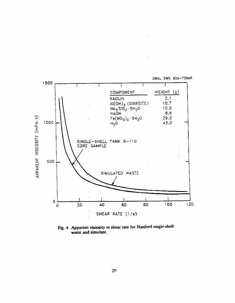
Rheological characterization of the waste samples is being done by PNL using a Haake RV 100 viscometer. A rheogram for one of the samples that has been characterized (homogenized 241-B-110 Core 1 composite) is shown in Fig. 4. The sample (which contains 21.1 wt % undissolved solids and 41.6 % centrifuged solids) has been characterized (at 31°C) as a yield-power-law fluid described by the following equation?

r,,, = 4.83 + 0.0448 ($)0.8817

where 7, = shear stress, (Pa) S = shear rate (s-*).

For purposes of comparison with the MVST data, 110-B Core 1 composite has a yield stress of 48 dyn/cm’, and if a power law coefficient of 1 is assumed, the plastic viscosity would be 45 cP.

Four simulants that exhibit rheological properties similar those of 110-B core samples were developed by PNL (recipes €3, F4, F5, and G) for possible use in the slurry test loop.28 The recipes €or preparing the simulants and the properties oE the simulants are given in Appendix A. All of the recipes used aluminum hydroxide (gibbsite), sodium

27

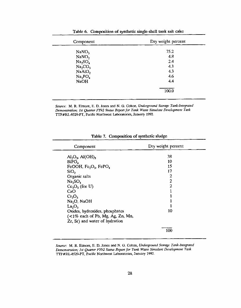
Table 6. Composition of synthetic single-shell tank salt cake

Component Dry weight percent

NaNO, NaNO, Na,SO, Na,CO, NaAIO, Na,PO, NaOH

75.2 4.8 2.4 4.3 4.3 4.6 4.4

100.0

Source: M. R. Elmore, E. D. Jones and N. G. Colton, Underground Storage Tank-Integrated Demonstration; 1st Quarter FY92 Status Report for Tank Waste Simulant Development Tayk 1TP#RL-8529-PT, Pacific Northwest Laboratories, January 1992.

Table 7. Composition of synthetic sludge

Component Dry weight percent

~ 2 0 3 , 4 O H ) 3 BiPO, FeOOH, Fe203, FePO, SiO, Organic salts Na,SO, Ce,O, (for U) CaO

Na,O, NaOH

Oxides, hydroxides, phosphates (< 1% each of Pb, Mg, Ag, Zn, Mn, Zr, Sr) and water of hydration

Cr@3

L a 2 0 3

38 10 15 17 2 2 2 1 1 1 1

10

100

Source: M. R. Elmore, E. D. Jones and N. G. Colton, Underground Storage Tank-Integrated Bemommation; 1st Quarter FY92 Status Repr t for Tank Waste Simuiant Development Task 1TP#RL-8529-PT, Pacific Northwest Laboratories, January 1992.

28

. rm" I3UU

1000

50C

(

ORNL DWG 92A-725AR

I 1 1 1 I

COMPONENT WEIGHT (9)

KAOUN 2.1 AI(OH), (GIBBSITE) 10.7

NaQH 8.6

43.0

No, Sios. 9HzO 10.0

Fe(N03j3 * 9H20 29.0

SINGLE-SHELL TANK B-110 CORE SAMPLE

SIMULATED WASTE

1 1 1 I 1 0 20 40 60 80 100 220

SHEAR RATE ( l / s )

Fig. 4. Apparent viscoSity vs shear rate for Hanford single-shell waste and sirnulaat

29

silicate, sodium hydroxide, ferric nitrate, and water. Recipe G included bismuth phosphate, while kaolin was used as a stand-in for bismuth phosphate in the F series recipes because of the expense and difficulty in obtaining large quantities of bismuth phosphate. The quantity of kaolin and water was varied in the F series siniulants. The mean particle sizes of recipes G and F5 were 42.6 pm and 36.9 pm respectively, as determined by a Brinkmann Particle Size Analyzer. The mean particle size ranged from 10.0 pm to 33.6 pm in four segments of the 110-B core sample as shown in Appendix k PNL suggested that recipe F5 be used as a base simulant and that the quantity of the components be varied to simulate a range of compositions. As shown in Fig. 4, the rheogram for simulant F5 is similar to that of core sample 110-B.

6. SUPERNATANT RHEOLOGY MEASUREMENTS

The major dissolved material in the supernatant liquid in the MVST and the soluble components (salt cake) in the Hanford single-shell tanks is sodium nitrate. The MVST also contains potassium nitrate and smaller amounts of carbonates, hydroxides, and chlorides. The Hanford salt cake contains sulfates, phosphates, nitrites, and aluminates. The supernatant in the WSTs is approximately 4 M in sodium and potassium nitrates. Efforts are under way to reduce the volume in the tanks by evaporation, which will increase the concentration of dissolved salts in the supernatant liquid.

Rheology measurements of simulated MVST supernatant and Hanford salt cake were made using a pipeline viscometer constructed of U4-h. (O.lt(O-in.-ID) tubing that was 10 ft long and by using the simulated supernatant compositions shown in Table 8. The results of calibration of the pipeline viscometer with water and sucrose solutions are shown in Fig. 5 and in Table 9. Viscosity measurements made using Brookfield and Fann viscometers are given in Table 9 for comparison with the pipeline viscometer measurements. Measurements were €or MVST supernatant at sodium and potassium nitrate concentrations (combined) of 4 M to simulate material presently in the tanks and at a concentration of 6 M to simulate conditions after the supernatant has been concentrated by evaporation. The rheology of the Hanford salt cake was also measured at 4 M and 6 M sodium nitrate concentrations. For comparison, the rheology of 4 M sodium nitrate was measured. The rheograms shown in Fig. 6 indicate that the simulated supernatant liquids for both the MVST and the Hanford salt cake are Newtonian (as expected) at the concentrations measured. The viscosity of the MVST 4 M simulant of 1.4 CP is somewhat less than those measured for actual supernatants that range from 1.7 to 2.2 cP. However, this may be within the range of the accuracy of the measurements.

7. CALIBRATION OF PIPELINE VISCOMETERS IN SLURRY TJ3T LOOP

To ensure proper operation of the pipeline viscometers in the slurry test loop, the viscometers were dimensionally measured and calibrated with Newtonian fluids for which the viscosity was known or could be verified by the use of laboratory viscometers (Brookfield and Fann). The pressure differential instruments used for pipeline viscometer

30

Table 8 Composition of mixtures used for supernatant viscosity measurements

Component 4 M" (a) 6 Ma (I&)

Melton Valley Storage Tank supernatant surrogate

NaN03

NaNO,

Na2S0,

Na2C03

NaAIO,

Na3P0,

NaOH

0.4

4.7

185.0

185.0

21.2

14.1

4.1

Hdord salt cake surrogate

341.8

21.8

10.9

19.6

19.6

20.9

20.0

0.6

7.1

278.0

278.0

30.9

21.1

6.2

512.7

32.7

16.4

29.3

29.3

31.4

30.0

Nitrate molarity.

31

Fig. 5. Pipeline viscometer (0.18-in. ID) calibration curves.

0 4M MVST 1.4

0 4M Hanford 1.9 6M Hanford 2.7

X 4M NaN03 1.3

Q) L

G I L a Q, z <n

0 200 400 600 800 1000 v-

Shear Rate (Us) Fig- 6. Rheogram for simulated Melton Valley Storage Tank ( M V S T )

supernate and Hanford salt cake.

32

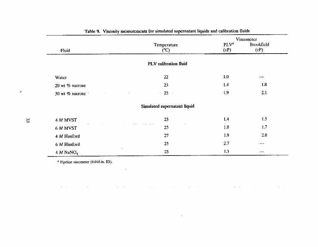
Table 9. ViscoSity measurements for simulated supernatant liquids and calibration fluids

Viscorne ter Temperature PLva Brookfieid

Fluid (“(3 (CP) ( C P )

BLV calibration fluid

Water

20 wt % sucrose

30 wt % sucrose

4 M MVST

6 M MVST

22

23

25

Simulated supernatant tiquid

25

25

4 M Hanford 27

6 M Hanford 25

1 .o 1.4

1.9

1.4

1.8

_-- 1.8

2.1

1.5

1.7

1.9 2.0

2.7 --- 25 1.3 --- 4 M NaNO,

a Pipeline viscometer (0.018-in. ID).

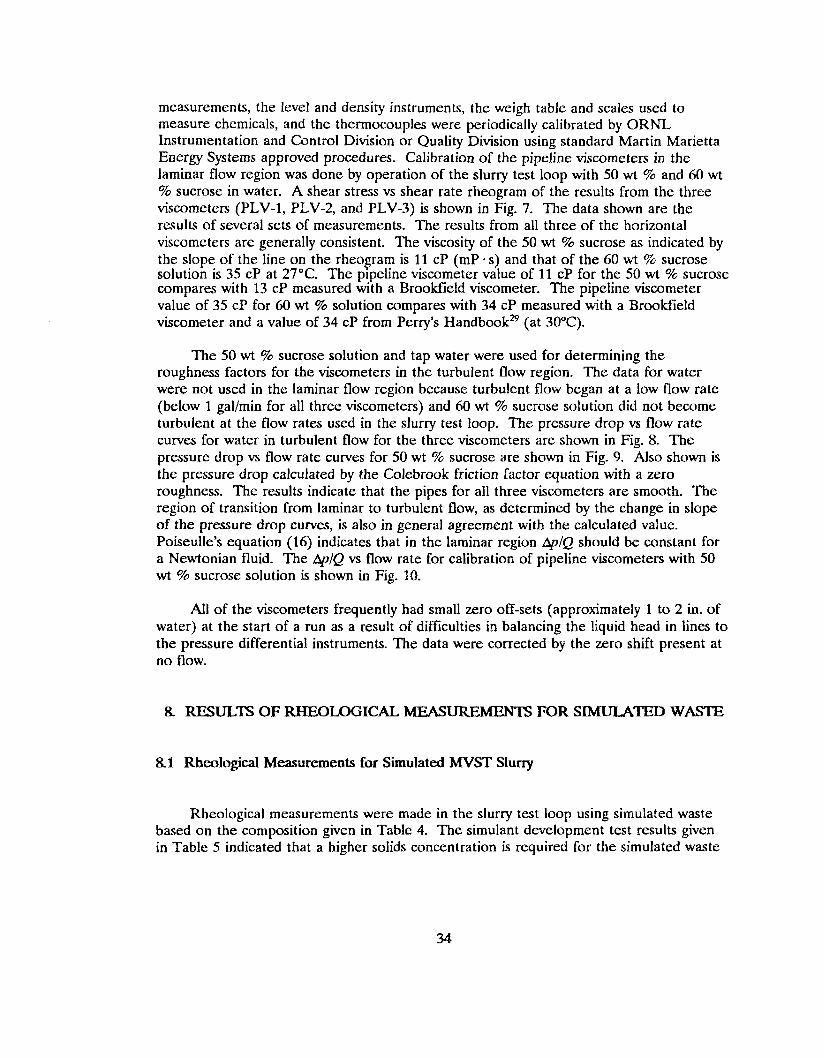
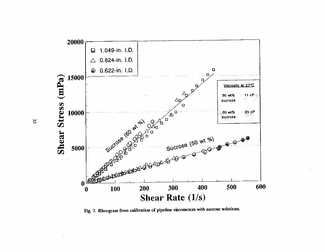
measurements, the level and density instruments, the weigh table and scales used to measure chemicals, and the thermocouples were periodically calibrated by ORNL Instrumentation and Control Division or Quality Division using standard Martin Marietta Energy Systems approved procedures. Calibration of the pipeline viscometers in the laminar flow region was done by operation of the slurry test loop with 50 wt % and 60 wt % sucrose in water. A shear stress vs shear rate rheogram of the results from the three viscometers (PLV-1, PLV-2, and PLV-3) is shown in Fig. 7. The data shown are the results of several sets of measurements. The results from all three of the horizontal viscometers are generally consistent. The viscosity of the 50 wt % sucrose as indicated by the slope of the line on the rheogram is 11 cP (mP .s) and that of the 60 wt % sucrose solution is 35 CP at 27°C. The pipeline viscometer value of 11 CP for the 50 wt % sucrose compares with 13 CP measured with a Brookfield viscometer. The pipeline viscometer value of 35 CP for 60 wt % solution compares with 34 cP measured with a Brookfield viscometer and a value of 34 CP from Perry's HandbookB (at 30'C).

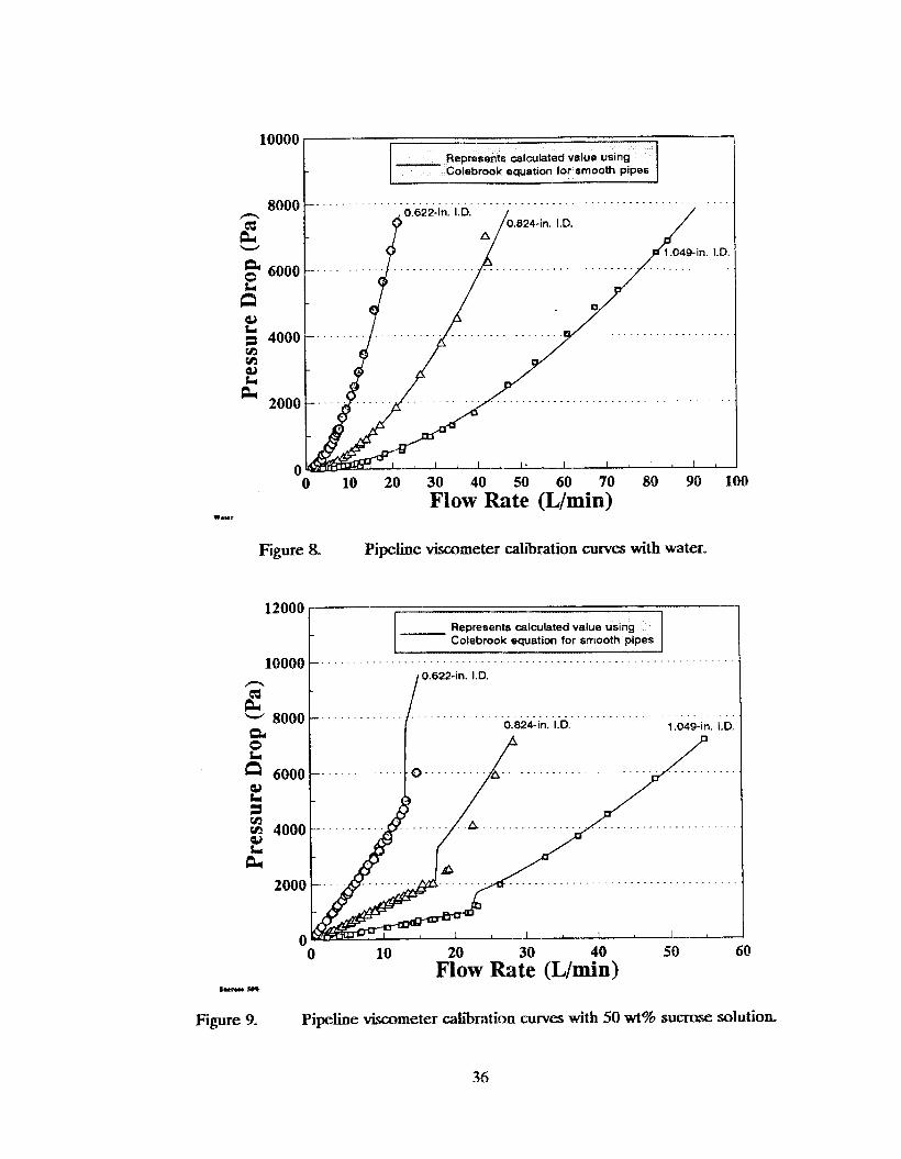
The 50 wt % sucrose solution and tap water were used for determining the roughness factors for the viscometers in the turbulent flow region. The data for water were not used in the laminar flow region because turbulent flow began at a low flow rate (below 1 gal/min for all three viscometers) and 60 wt % sucrose solution did not become turbulent at the flow rates used in the slurry test loop. The pressure drop vs flow rate curves for water in turbulent flow for the three viscometers are shown in Fig. 8. The pressure drop vs flow rate curves for 50 wt % sucrose are shown in Fig. 9. Also shown is the pressure drop calculated by the Colebrook friction factor equation with a zero roughness. The results indicate that the pipes for all three viscometers are smooth. The region of transition from laminar to turbulent flow, as determined by the change in slope of the pressure drop curves, is also in general agreement with the calculated value. Poiseulle's equation (16) indicates that in the laminar region Ap/Q should be constant for a Newtonian fluid. The AplQ vs flow rate for calibration of pipeline viscometers with 50 wt 96 sucrose solution is shown in Fig. 10.

All of the viscometers frequently had small zero off-sets (approximately 1 to 2 in. of water) at the start of a run as a result of difficulties in balancing the liquid head in lines to the pressure differential instruments. The data were corrected by the zero shift present at no flow.

8 RESULTS OF RHEOLOGICAL MEAS- FOR SIMULKED WASTE

81 Rheological Measurements for Simulated MVST Slurry

Rheological measurements were made in the slurry test loop using simulated waste based on the composition given in Table 4. The simulant development test results given in Table 5 indicated that a higher solids concentration is required for the simulated waste

34

ri

nd

-

--

0

I I

I

I I

0

#!

I

0

0

Q

a

a 0

Q 0

rjr)

0 0

d

err

35

10000 Represents calculated value using Colebrook equation for smooth pipe6

. . . . . . . . . . . . .....................

. . . . . . . . . . . . . . . . . . .

. . . . . . . . . . . . . . . . . . . . . . . . . . . . . . .

0 10 20 30 40 50 60 70 80 90 100 Flow Rate (L/min)

W.Y*

Figure 8 Pipehe viscometer calibration curves with water.

12000

10000 /1

E - 8000 a 0 Ll a 6000 Q) Ll

m 4)

a rn 4000

&

Represents calculated value using Colebrook equation for smooth pipes

0.622-in I.D.

i - . . . . . . . . . . . . . . . . . . . . . . . . . . . . . . . . . . . . 0.824-in. I.D.

. . . . . . . . . . . 1.044in. 1.B.

10 20 30 40 50 60 Flow Rate (L/min)

Figure 9. Pipeline viscometer calibration curves with 50 wt% sucrose solution.

36

0

- GO 0 oo

,

0

Q

rn 0

0

N

37

to give rheological properties similar to those of the sludge in the MVST. The first run in the test loop (MVST 1) was done with simulant containing a 65 wt % total solids (39 wt % undissolved solids). Run MVST 2 was done with the same batch of simulant but with the solids content reduced to 54 wt % total solids and 26 wt % undissolved solids by adding supernatant and removing sludge. A series of runs (MVST 3, 3A, 3B, and 3C) was made with the same simulant that had been adjusted to 57 wt % total solids (29 wt % undissolved) by adding sludge that had been previously removed. The temperature of the waste in the MVSTs varies with outside temperature from about 7°C to 21°C (45°F to 70°F). All of the tests except MVST 3A were made at room temperature (25°C). Run MVST 3A was made at 55°C to evaluate the effect of temperature on the rheology of the slurry. Also, for the final test the W S T simulated waste was passed through the IKA grinder to reduce the particle size of the slurry. Rheograms for the runs indicate that the slurry in all of the runs can be characterized as Bingham plastics. Pressure drop vs flow rate plots and rheograms for the runs are given in Appendix €3.

8.1.1 Run WST 1

Initially, approximately 40 gal of simulant containing 65 wt % total solids and 39 wt % undissolved solids was prepared for use in the test loop. Runs with MVST 1 slurry were made over a 5-d period to collect data, to test the equipment and instrumentation, and to evaluate the stability of the slurry. Rheological measurements were made by circulating the slurry sequentially through the pipeline viscometers at varying flow rates while recording flow rate, temperature, density, and pressure drop across the pipeline viscometers. At the concentrations, particle size, and temperatures studied, the slurry appeared to behave as a homogeneous fluid; therefore, no minimum transport velocity measurements were made. However, the waste tanks may contain larger particles that will require higher velocities for pipeline transport. During operation, data from the instruments were recorded on the computer disk at 5-s intervals. Flow rate vs pressure drop data for the pipeline viscometers in run MVST 1 are shown in Fig. 11.

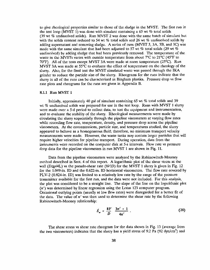
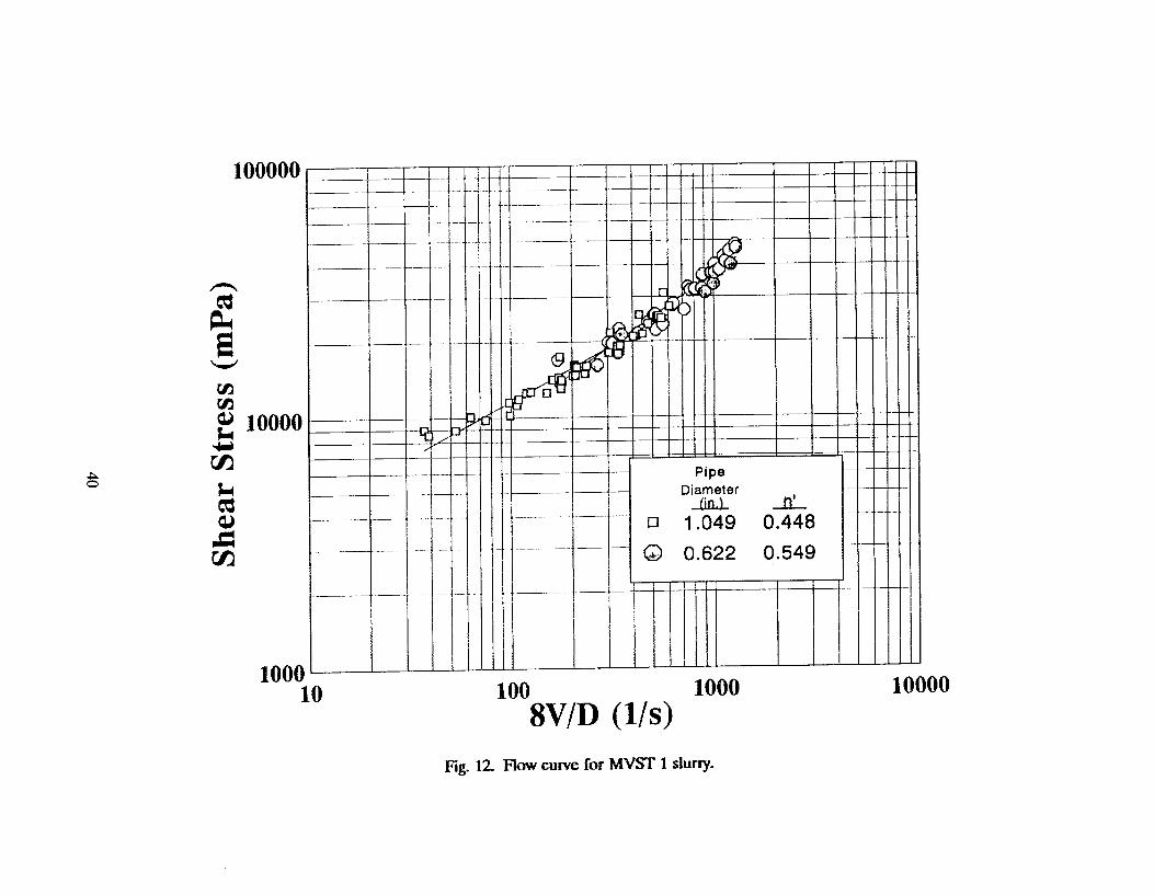
Data from the pipeline viscometers were analyzed by the Rabinowitsch-Mooney method described in Sect. 4 of this report. A logarithmic plot of the shear stress at the wall (DLpl4L) vs the pseudo-shear rate (8VID) for the MVST 1 slurry is given in Fig. 12 for the 1.049-in. ID and the 0.622-in. ID horizontal viscometers. The flow rate covered by PLV-2 (0.824411. ID) was limited to a relatively low rate by the range of the pressure transmitter available for the first run, and the data were not included. For this analysis, the plot was considered to be a straight line. The slope of the line on the logarithmic plot (n’) was determined by linear regression using the Lotus 123 computer program. Occasional outlying points (usually at low flow rates) were disregarded for a better fit of the data. The value of n’ was then used to determine the shear rate by the following Rabinowitsch-Mooney relationship:

The shear stress vs shear rate rheogram for the data shown in Fig. 13 (average from the two viscometers) indicates that the slurry has a yield stress of 9.2 Pa (92 dyn/cm2) and

38

100000

80000 n

0.622-in. I.D.

w

Q)

VI 1.049-in. I.D.

0 , I I I I I I 1 I I

0 20 40 60 80 100 120

FIow Rate (L/min) M-1

Fig. 11. Pressure drop vs flow rate for MVST 1 simulated sludge through pipeline viscometers.

40

I '

I

0

0

0

s 0

0

0

0

Wa

0

e

U

(I(

0 e

t? n

m

0

0

w

a

0

41

can be characterized as a Bingham plastic with a plastic viscosity of 25 mPa . s (25 cP). Although some of the settled sludge in the MVSTs has a considerably higher viscosity than that of the simulant, viscosity of the simulant is in the range that may be expected for pipeline transport of the slurry because up to three times as much supernatant as sludge may be used for mobilization (see Table 3). The pipeline transfer of the same general type of slurry from the Gunite tanks to the MVSTs was done at an apparent viscosity of about 16 CP (at a shear rate of 510 s - ' ) . ~ In tests with Hanford double-shell tank slurry in 1984, it was determined that the effective pipeline viscosity of the most concentrated evaporator fluid was less than 56 C P . ~

8.12 RunMVST2

To study the effect of a slurry with lower solids content, a simulant was made from MVST 1 with a portion of the sludge removed and additional supernatant added. Run MVST 2 was made at a slurry concentration of 54 wt % total solids and 26 wt % undissolved solids. The pressure drop curves and rheograms obtained with the 0.62241. ID and the 0.0824-in. ID viscometers are shown in Figs. B.3 and B.4 in Appendix B. The results from the 1.049-in. ID viscometer were not used because of excessive zero shift of the pressure transmitter. Rheograms for run MVST 2 indicate that the slurry can be characterized as a Bingham plastic fluid having plastic viscosity of 7.8 mPa.s and a yield stress of 0.9 Pa.

8 1 3 Rum W S T 3,3A, 3B, and 3C

For the third series of runs (MVST 3, 3 4 3B, and 3 6 ) , the solids concentration in the slurry was increased to 57 wt % total solids and 29 wt % undissolved by adding concentrated sludge from run MVST 1. The density of the slurry was 1.5 g/cm3. Runs were made in the slurry test loop at room temperature 25°C (run MVST 3) and at 55°C (run MVST 3A). After heating the slurry (in run MVST 3A), a second run was made at 25°C (run MVST 3B) to determine if the properties of the slurry were changed by heating. After run MVST 3B, the slurry was passed through the IKA grinder 10 times to reduce the particle size (and run as W S T 3C). Pressure drop vs flow rate curves and rheograms for these runs are shown in Figs- B.5 through B.12 in Appendix B. The data on the rheograms are represented by a straight line indicating Bingham plastic behavior. The plastic viscosity and yield stress for run MVST 3 (made at 25°C) were 7.9 mPa.s and 1.6 Pa, respectively. Measurements of the same slurry at 55°C resulted in a reduction in plastic viscosity to 3.7 mPa - s and an increase in yield stress to 3.9 Pa (data from the l-in. viscometer were not used). No significant change in the density of the slurry occurred from heating the slurry from 25 to 55°C. The plastic viscosity and yield stress of slurry after cooldown to 25°C were 8.9 n P a - s and 1.9 Pa, which are near the values measured before heatup, indicating that the changes in plastic viscosity and yield stress at the higher temperature were likely a result of temperature effects rather than chemical changes in the slurry.

After run MVST 3B was completed, the particle size of the slurry was reduced by making 10 passes through the three-stage IKA grinder at a nominal flow rate of 14 gal/min. Grinding of the slurry resulted in an obvious increase in settling time. Particle size measurements with a Northrup Microtrac laser scanner showed a reduction in the

42

maximum particle size of the slurry from 42 pm to 30 pm after two passes and a reduction to 15 pm after 10 passes through the grinder. After grinding (run MVST 3C) the plastic viscosity of the slurry remained approximately the same at 8.2 to 8.9 mPa s while the yield stress increased from 1.9 Pa to 3.8 Pa. This is the same general type of response observed in the laboratory grinding test shown in Table 5. The rheological measurements for all of the runs with MVST simulated waste are summarized in Table 10.

Average values of yield stress and ptastic viscosity results obtained experimentally in the laminar flow region were used to calculate the transition region from laminar to turbulent flow and the pressure drop in the turbulent flow region using the YPLPIPE computer program. The calculated pressure drop vs flow rate values for run MVST 1 give good agreement with experimental values as shown in Fig. 11. A comparison of the calculated and measured pressure drop curves for runs MVST 2 through MVST 3C is shown in Figs. €3.3, B.5, B.7, 3.9, and B.11 in Appendix €3.

82 Rheological Measurements of Simulated Hanford Singleshell Tank Waste

Rheological measurements were made in the slurry test loop using simulated Hanford single-shell tank waste prepared by recipe F5 (described in Appendix A) that has rheological properties similar to single-shell tank sample 241 43-1 10. The apparent Viscosity of the larger batch of simulant was lower than that of material prepared in small batches; however, the viscosity was in the range expected for pipeline transport. The first series of rheological measurements (runs H-1, H-2, H-3, and H-4) was made in the slurry test loop with simulant containing approximately 42 wt % total solids and 25 wt % undissolved solids and a density of about 1.36 g/cm3. The second series of measurements (runs H-5, H-6, and H-7) was made with slurry from the first series of runs that had been diluted with supernatant to give a total solids content of about 42 wt %, an undissolved solids content of 23 wt %, and a density of about 1.36 g/cm3. Pressure drop vs flow rate measurements were made in both laminar and turbulent flow using the three horizontal pipeline viscometers.

The first measurements with concentrated slurry (run H-1) were made at ambient temperature 25°C. This was followed by measurement (run H-2) made at 50"C, which is approximately the temperature at which pipelines for Hanford single-shell waste will operate (because of the heat generated by radioactive decay). This run was followed by two additional runs (H-3 and H-4) made primarily to determine if the properties of the simulant were changed by heating or due to aging.

To obtain information about the effect oE solids concentration on the rheological properties, the simulant used for runs H-1 through H-4 was diluted with supernatant. Run H-5 was made at 25°C with the diluted slurry. Run H-6 was made with the same slurry at 50°C. This was followed by run H-7 at 25°C made with the same slurry to determine if the rheological properties of the s i u q were changed by heating.

Data from the pipeline viscometers were analyzed by the Rabinowitsch-Mooney relationship previously described. Typical pressure drop vs flow rate curves and rheograms

43

Table 10. Summary of rheological measurements with Melton Valley Storage Tank simulant in the slurry test loop

Undissolved Yield Temperature Density Total solids solids Plastic stress

Run number (“C) (g/cm3> (wt (wt %) viscosity (Pa)

MVST 1 25 1.63 65 39 25 9.2

MVST 2 25 1.49 54 26 7.8 0.9

MVST 3 25 1.54 57 29 7.9 1.6

MVST 3A 55 1.51 57 29 3.7 3.9

MVST 3B 25 1.5 57 29 8.9 1.9

MVST 3C 25 1.5 57 29 8.2 3.8

(for run H-2 ) are shown in Figs. 14 and 15. Pressure drop vs flow rate curves, rheograms, and a tabulation of the data for all runs are given in Figs. B.13 through B.26 in Appendix B.

Evaluation of the shear rate vs shear stress data indicated that the slurry at all of the conditions studied could adequately be represented by a Bingham plastic model. Under the conditions studied, the slurry appeared to behave as a homogeneous slurry, and no minimum transport velocity was observed. The rheological measurements for the ruins are summarized in Table 11.

As shown in Table 11, the values obtained from the different viscometers are generally consistent. The variation between viscometers is generally within the accuracy of the equipment. Wall slip was not detected within the scatter of the data after analysis using the method outlined by Brown.31

Average values of the plastic viscosity and yield stress obtained in laminar flow from all viscometers were used in the YPLPIPE computer program to calculate pressure drop in turbulent flow and the critical Reynolds nurnber €or transition from laminar to turbulent flow. The calculated result shown as solid lines on the pressure drop vs flow rate curves indicates good agreement with measured values for all runs. Calculated and measured friction factors and critical Reynolds numbers are shown in Fig. 16.

Increasing the slurry temperature from 25°C to 50°C resulted in a decrease in the plastic viscosity (average for the three Viscometers ranged from about 5.4 mPa - s to 3.5 mPa - s and from 4.1 mPa - s to 29 mPa + s) and essentially no chan e in the eld stress

4 resulted in only a small change in undissolved solids (from 25 wt % to 23 wt %). The dilution resulted in a decrease in both the plastic viscosity and yield stress of the slurry, as shown in Table 11. However, the limited range of temperature and concentration covered is not sufficient to draw general conclusions on the effect of temperature and concentration.

in the two runs. Dilution of the slurry with 20 L of supernatant a H 2 ter run

The slurry appeared to be relatively stable over the period that the runs were made and as a result of heating the slurry to 50°C. Only small changes in properties were observed between the initial and final runs at the same concentration. Particle size analysis by a k e d s and Northrup Microtrac analyzer indicated a decrease in the size of the lar e particles (from 90 wt % less than 25 pm to 90 wt % less than 14.3 pm) but on1

less than 4.3 pm) between the initial and final runs. a smaf ig decrease in the mean particle diameter (from 50 wt % less than 5 pm to 50 wt 7 o

45

nd

m

k

Shea

r S

tres

s (m

Pa)

F

F

N

V

I 0

VI

0

0

0

0 0

Q

0

0

0

0

0

0

0

0

0

I I

I I

Pre

ssur

e D

rop

(Pa)

m

0

a 0

0 0

0 0

0

0

Table 11. Summary of rheological measurements with Hanford simulated waste

Plastic viscosity (mPa s) Yield stress (Pa)

Run Temp. Density Total number “c (g/cm’) solids(wt %) PLV-1” PLV-2b PLV-3‘ Fannd PLV-1 PLV-2 PLV-3 Fann

2s 1.36 42.0 5.2 5.1 6.0 6.7 11.9 13.4 13.6 12.8 H-1

50 1-35 42.3 4.2 2.7 3.7 9.9 12.2 11.3 H-2

El-3 25 1.36 42.4 8.1 6.0 6. f 7.2 9.8 8.7

H-4 25 1.37 43.5 7.7 4.1 4.7 8.8 12.4 11.0

Run H 4 slurry diluted with 20 L of supernatant

8.3 6.8 H-5 25 1.36 41.7 3.6 3.9 4.7 4.6 5.9 8.2

H-6 50 1.36 42.7 2. I 2.1 4.4 6.6 8.4 7.9

H-7 25 1.37 43.5 5.4 6.3 5.5 5.8 7.8 8.3 P 4

“1.049-in. ID by 10-ft.-long horizontal pipeline viscometer. *0.824-in. ID with 10-ft.-long horizontal pipeline viscometer. ‘0.622-in. ID with lO-ft.-long horizontal pipeline viscometer. dModel 35A viscometer.

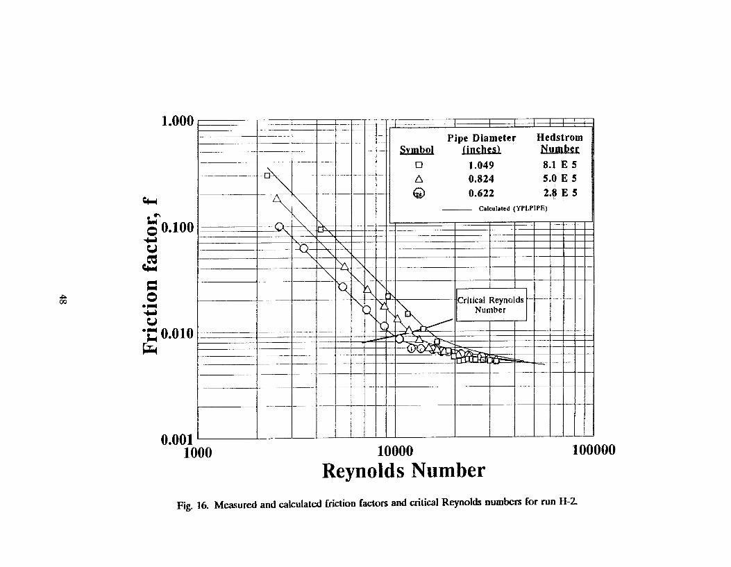
..I

a

0

L

li

0

rl

0

9

i

0

0

0

0

0

F-4

a a

0

0

rl

9. PERFORMANE OF EQUIPMENT AND INSTRUMENTA~ON

The equipment and instrumentation in the slurry test loop performed essentially as designed. No major equipment or operational difficulties such as plugging were experienced. Measurement of the flow rate by use of the weigh table (WT-205) confirmed that the magnetic flowmeter (FE-125) gave results that were in agreement within about 5% at flow rates above 1 gal/min. Slurry density measurements by the Micromotion mass flowmeter w-130) were in agreement with density results by pycnometer measurement. The Moyno and centrifugal pumps performed satisfactorily. The differential pressure instrument with diaphragm seals performed satisfactorily; however, some difficulties were encountered in balancing the zero reading €or measurements at low differential pressures. Also, temperature control was difficult to maintain when the loop was operated near ambient temperature because of the heat input of the pumps and the small temperature difference between the loop and the cooling water. This was corrected by the installation of a small surplus refrigerated cooling unit. The data-cdection system (GenesisTM software) worked well. The data collected in files were easily transferred to floppy disks for analysis by standard spreadsheets on a personal computer.

10. SUMMARY AND CONCLUSIONS

The objective of the fluid dynamic studies was to identify or develop correlations for predicting the flow parameters needed for the design and operation of slurry pipeline transport systems for the radioactive waste slurry stored in the Hanford single-shell tanks and the ORNL h4VSTs. Nonradioactive simulated waste with chemical compositions and rheologicai properties similar to the Hanford single-shell tank waste was developed by PNL, and simulated waste with properties similar to the MVST waste was developed at ORNL for use in the study.

A slurry test loop was constructed to study the flow properties of the simulated slurry and to evaluate equipment and instrument performance for handling slurry. Rheological properties of slurry were studied by circulating the slurry through three sizes of pipeline viscometers (constructed 1D-, 3/4-, and 1-in. schedule 40 pipe) at rates up to 35 gaUmin. Runs were made with ORNL simulated waste at concentrations of 54 wt %, 57 wt %, and 65 wt % total solids and at temperatures of 25°C and 55°C. Grinding was done before one run to study the effect of reduced particle size. Runs were made with Hanford simulated waste at 42 wt % to 43 wt % total solids and at temperatures of 25°C and 50°C. The rheology of simulated Hanford and ORNL waste supernatant solution was also measured at 4 A4 and 6 M nitrate concentrations.

Data from the studies in the test loop indicated that the slurry for both the ORNL and Hanford simulated slurry was non-Newtonian and could be represented by the Bingharn plastic model. At the conditions studied, the yield stress of the O W L waste ranged from 0.9 Pa to 9.2 Pa, and the plastic Viscosity ranged from 4 mPa * s to

49

25 mPa . s. The yield stress of the Hanford simulated waste ranged from 7 Pa to 13 Pa, and the plastic viscosity ranged from 3 mPa * s to 7 mPa - s. The waste behaved as homogeneous slurry under all of the conditions studied. The supernatant solution (at concentrations of 4 M and 6 M nitrate) was Newtonian as expected, with viscosities ranging from 1.3 mPa * s to 2.7 mPa s.

Mathematical models and commercially available computer programs for calculating pressure drop, critical Reynolds numbers, and minimum transport velocities were identified and described by a slurry transport consultant (Richard W. Hanks Associates). Measured values of pressure drop and critical Reynolds numbers showed good agreement with values calculated using a commercially available computer program (YPLPIPE).

Based on the limited range of variables studied, existing non-Newtonian models and correlations for predicting pressure drop and the region of transition from laminar to turbulent flow appear to be good for modeling the type of waste stored at Hanford and ORNL; however, additional studies over a wider range of compositions, particle sizes, and concentrations are recommended. Additional work is needed to develop computer programs for analysis of data from pipeline viscometers and to modify existing programs for calculating deposition velocity for non-Newtonian fluids and fluids that contain particles of more than one density. Although the slurries used in these tests behaved as homogeneous slurries and no information on minimum transport velocity was obtained, the actual waste may contain larger particles that will have minimum transport velocities.

The use of chemical surrogates appears to be a promising way to simulate the rheological properties of the actual waste. However, only a limited amount of rheological data is currently available for the actual waste for comparison. The rheological properties of material prepared in larger batches did not always duplicate that prepared on a small scale. Additional work is recommended on chemical simulant development to identify the variables that are important in determining rheological properties over a wide range of compositions. The equipment and instruments used in the slurry test loop operated satisfactorily. Additional testing with larger pipe sizes and longer runs is recommended to evaluate flow correlations for scale-up.

ACKNOWLEDGEMENTS

The authors wish to express their appreciation to summer participants Seann M. Reed and Christopher E. Lockwood for their assistance in simulant development, operation of the slurry test loop, and computer programming for data analysis. The authors also wish to express their appreciation to M. D. Boring, J. J. Perona, and J. L. Snyder for their helpful comments in reviewing the report and to Roger L. Gilchrist, Manager, Underground Storage Tank-Integrated Demonstration for his leadership and support of the project.

50

REFERENCES

1.

2.

3.

4.

5.

6.

7.

8.

9.

10.

11.

12.

13.

14.

15.

16.

17.

18.

19.

T. D. Hylton, Personal Communication, August 31, 1992.

F. R. Ruppel, Personal Communication, September 1992.

k H. P. Skelland, Non-Newtonian Flow and Heat Transfer, J. Wiley, New York, 1967.

3. Rabinowitsch, &it. Physik Chem. A145 (1) (1929).

M. Mooney, J. Rheol. 2 (210) (1930).

V. L. Streeter, Fluid Mechanics, 5th Ed., McGraw-Hill, New York, 1971, p. 292.

R. W. Hanks and D. G. Sloan, Proc 6th Int '1 Tech. Conf on Slurry Tramp., Las Ve as, March 26-28, 1981, pp. 107-120, Slurry Transport Association, Washington, D.8.

E. J. Wasp, et al., Pipeline News, July 1963, p. 20.

R. W. Hanks, AIChE Journal 9,306-309 (1963).

R. W. Hanks and B. H. Dadia,AfChEJoumal 17, 554-557 (1971).

D. G. Thomas, AIChE Journal 6,631-639 (1960).

R. W. Hanks, "Principles of Slurry Pipeline Hydraulics," in Encyclopedia of Fluid Mechanics, Vol. V (Slurry Flow Technology), N. P. Cheremisinoff, Ed., Gulf Publishing Co, Houston, 1986, pp. 213-276.

A. B. Metzner and J. C. Reed, AIChE Journal 1, 434 (1955).

R. W. Hanks, Proc. 4th Int'l Tech. Con& on Sluny Tmnsp., Las Vegas, March 28-30, 1979, pp. 91-101, SIurry Transport Association, Washington, D.C.

N. W. Ryan and M. M. Johnson, AIChE Journal 5,433 (1959).

R. W. H a n b , AIChE Jouml9,45-48 (1963).

R. W. Hanks and B. L. Ricks, J. Hydronautiks, 9, 39-44 (1975).

R. W. Hanks, Proc. 5th Int'l Con$ on Hydraulic Tramp. of Soli& in Pipes, Hannover, Germany, May 8-11, 1978, Pub. by BHRA Fluid Engineering, Cranfield, U.K., pp. C2-C25 (1978).

R. Durand, Roc. Minnesota Int'l Hydraulics Convention, September 1-4, 1953, p. 89, University of Minnesota.

51

20. R. W. Hanks, "Development of Slurry Viscometry Data Analysis Procedure," Richard W. Hanks Associates Consulting Report to Battelle PNL, Contract No. B-R6822-A-U, April 22, 1987.

21. M. B. Sears, J. L. Botts, R. N. Ceo, J. J. Ferrada, W. H. G r i s t , J, M. Keller, and R. L. Schenley, Sampling and Analysis of Radioactive Liquid and Waste Sludges in the Melton Valley and Evaporator Facility Storage Tanks at O W L , ORNWZTvf-11652, Oak Ridge National Laboratory, Oak Ridge, Tenn., September 1990.

22. R. N. Ceo, M. B. Sears and J. T. Shor, Physical Characterization of Radioactive Waste Tank Sludges, ORNI.JTM-11653, Oak Ridge National Laboratory, Oak Ridge, Tenn., October 1990.

23. D. W. Turner, J. B. Berry, and J. W. Moore, "An Overview of the ORNL Waste Handling and Packaging Plant," Waste Management '90, February 1990.

24. H. 0. Weeren, Sluicing Operations at Gunite Waste Storage Tanks, FW-84142, September, 1984

25. k J. Mattus, Oak Ridge National Laboratory, Personal Communication to J. B. Berry, August 13, 1990.

26. M. R. Elmore, E. 0. Jones, and N. G. Colton, Underground Storage Tank-Integrated Demonstration, 1st-Quarter FY92 Status Report for Tank Waste Simulant Development Task, 'ITP#RL-8529-PT, Pacific Northwest Laboratories, January 1992.

27. Personal communication from E.O. Jones to J.B. Berry, Oak Ridge National Laboratory, October 21, 1991.

28. N. G. Colton and M. R. Elmore, Pacific Northwest Laboratories, Letter Report to E. L. Youngblood, Oak Ridge National Laboratory, October 15, 1992.

29. Chemical Engineem' Handbook, Fourth Edition, John H. Perry Ed., McGraw Hill Book Company, p. 3-201.

30. Personal communication with G. J. Rust and D. C. Bjorklund, Westinghouse Hanford Co., February 1992.

31. Slurry Handling Design of Solid-Liquid Systems, N. P. Brown and N. I. Heywood, Eds., Elsevier Science Publishers LTD, 1991, pp. 71-73.

52

APPENDIX A

Deveiopment of Sirnulants for Hanford Single-Shell Waste Tanks

Report prepared by

Battelle Pacific Northwest Laboratories P. 0. Box 999

Richland, Washington 99352 under

Subcontract No. lOXSUil3V

for

OAK RIDGE NATIONAL LABORATORY Oak Ridge, Tern.

Managed by Martin Marietta Energy Systems, Inc.

Pacific Northwest Laboratories P.O. Box 999 Richland, Washington U.S.A. 99352 Telephone (509,376 - 4252

October 15, 1992

Mr. L1 oyd Youngbl ood Oak Ridge National

P.O. Box 2008 Oak Ridge, TN 37831-6330

Laboratory MSIN 6330

Dear Mr. Youngblood:

The objective for DeveloDment of Simulants for Hanford Sinqle-shell Waste Tanks was to develop non-hazardous simulants that have the following characteristics: characteristics similar to those measured for actual waste samples, (b) are based on formulations that can be extrapolated to simulate the rheological properties of the range of waste compositions contained in the single-shell tanks, and (c) are suitable for use in a slurry test loop (approximately 50 gallon capacity) to study the pipeline transport of waste slurries.

(a) have apparent viscosity versus shear rate

With the above-stated objectives in mind, recipes for Hanford single-shell tank (SST) physical simulants were derived, and simulants were prepared. The rheological characteristics o f the simulants were compared with Hanford SST ; t , l - B - l l O , and the recipes were adjusted until the simulant displayed apparent scosity versus shear rate characteristics similar to the waste sample,

Four recipes for simulants that exhibited similar rheological characteristics t o 241-8-110 are outlined in Attachment 1. The estimated compositions o f the simulants, along with the composition o f 241-B-110 and an average SST sludge waste (based on the analyses o f 18 SSTs), are listed in Attachment 2.1. Note that recipe "GI' contains the bulk constituents found in sludge while recipes ' IF-3" through " F - 5 " contain the bulk constituents with the exception o f bismuth and phosphate. Kaolin was substituted for bismuth phosphate in the 'IF" series simulants due to the high cost of the chemical ($150/100g). For your information, the range of major constituents found in the 18 analyzed SSY wastes is also provided in Attachment 3 ,

The simulants are prepared from five starting materials plus water, and scale- up o f the recipe t o prepare 50 gallons of simulated sludge should be fairly straight forward. Two points to note in the preparation o f the simulant: (1) Good dissolution and mixing should be maintained to keep particle sizes as small as possible, and (2) sodium hydroxide and the iron nitrate solution should be added to the mixture slowly, as heat is generated with the additions. The chemical constituents in the sludge are not federally regulated to the best o f my knowledge (sodium nitrate is (40 wt% wet sludge, and at this concentration is not considered an oxidizer); however, the pH of the sludge is 2 12.5, and the sirnulant is thereby considered hazardous due to its corrosive nature.

54

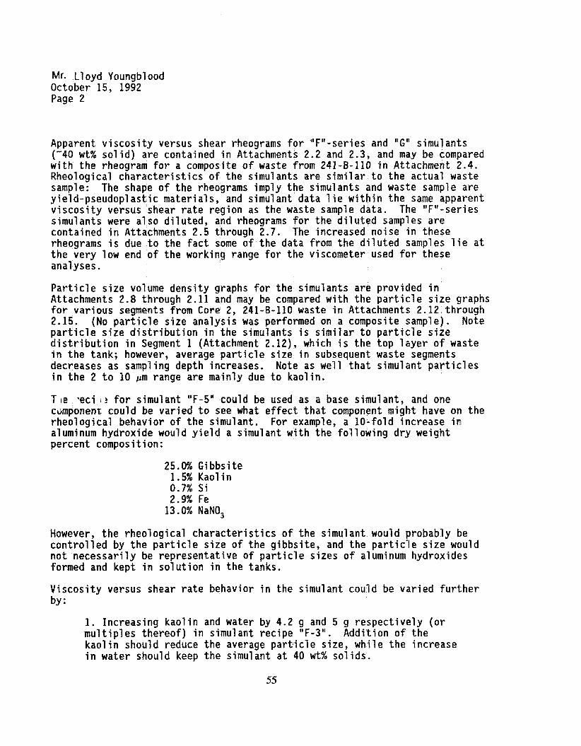
Mr. L1 oyd Youngbl ood October 15, 1992 Page 2

Apparent viscosity versus shear rheograms for "F"-series and "G" simul ants (-40 wt% solid) are contained in Attachments 2.2 and 2.3, and may be compared with the rheogram for a composite of waste from 241-8-110 in Attachment 2 .4 . Rheological characteristics of the simulants are similar to the actual waste sample: The shape o f the rheograms imply the simulants and waste sample are yield-pseudoplastic materials, and simulant data 1 i e within the same apparent viscosity versus shear rate region as the waste sample data. The "F"-series simulants were also diluted, and rheograms for the diluted samples are contained in Attachments 2.5 through 2.7. The increased noise in these rheograms is due to the fact some of the data from the diluted samples lie at the very low end of the working range for the viscometer used for these analyses.

Particle size volume density graphs for the sirnulants are provided in Attachments 2.8 through 2.11 and may be compared with the particle size graphs for various segments from Core 2, 241-8-110 waste in Attachments 2.12 through 2.15. (No particle size analysis was performed on a composite sample). Note particle size distribution in t h e simulants is similar to particle size distribution in Segment 1 (Attachment 2.12), which i s the top layer o f waste in the tank; however, average particle size in subsequent waste segments decreases as sampling depth increases. Note as well that simulant particles in the 2 to 10 pm range are mainly due to kaol in.

T l e *eci 2 for simulant "F-5" could be used as a base simulant, and one ccimponent could be varied to see what effect that component might have on the rheological behavior of the simulant. For example, a 10-fold increase in aluminum hydroxide would yield a simulant with the following dry weight percent composition:

25.0% Gi bbsi te 1.5% Kaolin 0.7% Si 2.9% Fe 13 .OX NaNO,

However, the rheological characteristics of the simulant would probably be controlled by the particle size of the gibbsite, and the particle size would not necessarily be representative of particle sizes o f aluminum hydroxides formed and kept in solution in the tanks.

Viscosity versus shear rate behavior in the simulant could be varied further by :

1. Increasing kaolin and water by 4.2 g and 5 g respectively (or multiples thereof) in simulant recipe ' IF-3". Addition of the kaolin should reduce the average particle size, while the increase in water should keep the simulant at 40 wt% solids.

55

Mr. L1 oyd Youngbl ood October 15, 1992 Page 3

2. Increasinq the ercent solids concent ation to 40 wt% sol ids .) Based on the-analyses of 18 SST wastes, solids in sludge generally range from 40 to 60 wt%.

Within reason, we believe simulants prepared from the recipes provided, along with the above-mentioned variations, are representative of a range of existing Hanford tank wastes. However, because o f very 1 imited rheological characterization data for tank wastes, we are unable to quantify the extent of this range. simulants were developed to model the properties of wastes as they exist in the tanks, the component concentrations and rheological behavior do not necessarily reflect the properties of "retrieved" waste that would then be transported through pipelines. The method of retrieval (especially the amount of dilution necessary) will undoubtedly impact the waste composition and behavior. This uncertainty would need to be factored into your testing.

Additionally, we would like to point out that since these

We have appreciated the opportunity to work with you on this effort, and we hope our input will be helpful to your research. I f we may be of further assistance, please contact us.

Very truly yours,

N. Researc G * Tton Scientist Project Manager

Attachments: 17

56

Attachment 1: Recipes for Hanford Single-shell Tank Physical Simulants

SST PHYSICAL SIMULANT RECIPES

SST Simulant F-3

To 30 mL H,O add in the following order while stirring:

8.38 g Kaolin

8.60 g NabH

10.65 g Gibbsite (Al(OH),) 10.01 g Na SiO,.9 H,O

Dissolve 28.96 g Fe(NO3),-9 H,O in 20 mL H,O and add to above.

SST Simulant F-4

To 25 mL H,O add in the following order while stirring:

4.19 g Kaolin

8.60 g NabH

10.65 g Gibbsite (Al(OH),) 10.01 g N a SiO,.9 H,O

Dissolve 28.96 g Fe(NO,),.9 H,O in 20 mL H,O and add to above.

SST Simulant F-5

To 22.5 mL H,O add in the following order while stirring:

2.10 g Kaolin

8.60 g NabH

10.65 g Gibbsite (Al(OH),) 10.01 g Na SiO, .9 H,O

Dissolve 28.96 g Fe(N03)3.9 H,O in 20 mL H,O and add t o above.

SST Simulant 6

To '40' mL H,O add in the following order while stirring:

2.80 g BiPO,

8.60 g NabH

10.65 g Gibbsite (Al(OH),) 10.01 g Na Si03-9 H,O

28.96 g Fe(NO,),.9 H,O

Amount of water approximated; further work on simulant discontinued due to high price o f BiPO, ($150/100g).

57

Attachment 2.1: Estimated Compositions and Physical Properties (Simulants and SST 241-B-110)

Estimated Compositions (dry weight %)

F-3 F-4 F-5 G 8-110 SST I' Avq 'I S ST

16.0% KaBl in' 9.5% Kaylin' 5.0% Kaylin' 6.1% B i PO, 6.3% BiPO, 6.2% BiPO, 6.7% A1 7.9% A1 8.3% AI 7.5% A1 0.1% A1 6.8% A1 1.9% s i 3 2.3% S i 3 2.4% S i 3 2.0% S i 2.:,% Si 5.4% S i 7.7% Fe 9.1% Fe 9.6% Fe 8.7% Fe 4.8% Fe 4.9% Fe

35.0% NaNO, 42.0% NaNB, 44.0% NaNO, 40.0% NaNO, 54.0% NaNO, 45.0% Soluble Salts4

'Kaolin substituted for BiPO, due to high cost o f BiPO, ($150/100 g) *A1 from kaolin not included i n % 3 S i from kaol i n not included in % 41ncludes sodium nitrate, nitrite, sulfate, carbonate, phosphate; note simulant samples contain only sodium nitrate for simplicity.

Phvsical Properties

F -3 F-4 F- 5 G 5-110 SST

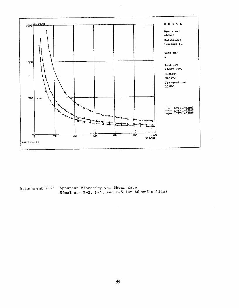
mPas1 I

URRKE Rot 2.5

H A A K E

Operator: elrnore

Substance: lwsrtsir F3

Test No.: 1

T e s t of: 24.Sep 1992

Systen: MS/SV2 Temperature: 23.0OC

-3- LYF3-4Q.P.01 -4- LYF4-40.ROT -5- LYF5-48.ROT

I

Attachment 2.2: Apparent Viscos i ty vs. Shear Rate Simulants F-3, F-4, and F-5 (at 40 wt% solids)

59

150

1001

50

: m P a s I

W A K E Rot 2.3

H R R K E

Operator: elmore

Substance: lysstsim-G

Test No.: 1

T e s t of: 14.Sep 1992

System: M W S V 2

Temperature:

23'C

--- LYSST-G.ROT

I

At tachmen t 2.7: Apparent Viscosity vs. Shear Rate Simulant G (40 wt% s o l i d s )

a

-=--e--

--+--%-

I fil/

169.6--,

H A A K E

Operator: elmore

Substanca: l y s t s i m F3

Test No.: 1

Test of: 24.Sep 1992

SyStQm: n5/sv2 Temp@raturP: 23.0%

-a- LYF5-40.ROT - ~

-b- LYF3-35.ROT -c- LYF3-30.ROT 4- LYF3-25.ROT

3

Attachment 2.5: Apparent V i scos i ty vs. Shear Rate Simulant F-3 a t 40 , 35, 30, 25 w t % solids

61

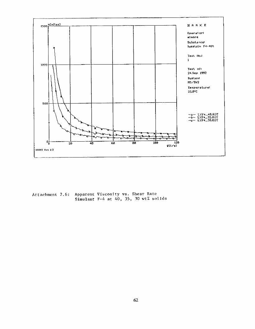
HAAKE R e t 2.5

60 80 I

H R R K E

Operator: elmore

Substance: lysstsim F4-48%

Te5t No.: 1

T e s t OD 24.Sep 1992

Svstem: M5/SV2

Temperature: 23.0'C

-a- LYF4-40.ROT -b- LYF4-35.ROT -c- LYF4-30.ROT

3

Attachment 2.6: Apparent Viscosity vs. Shear Rate Simulant F-4 at 40 , 35, 30 wt% s o l i d s

62

Attachment 2 . 4 : Apparent V i s c o s i t y vs. Shear Rate Single-shell Tank 241-B-110, Composite

L

1500

1000

500

0 I I I I ..a

0

- - _ - -

'1. ,

20 40 60 80

Shear Rate, sec-'

100 120

63

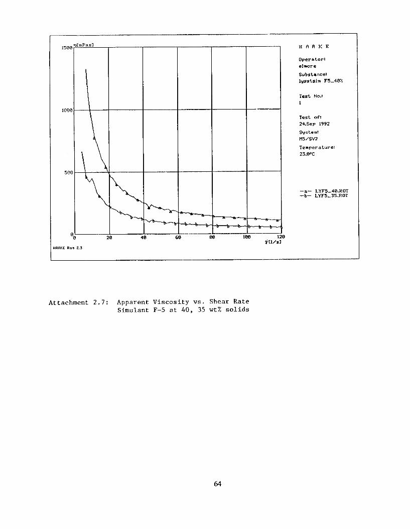
1500

1000

500

0 I 100 1

4CICIKE Roo 2.3

H A A K E

Operator: clmore

Substance: lysstsim F5-40%

Test No.: 1

Test OF: 24.Sep 1992

System: M5/SV2

Temperature: 23.0OC

-a- LYF5-40.ROT -b- LYF5-35.P.OT

Attachment 2.7: Apparent Viscosity vs. Shear Rate Simulant F-5 at 4 0 , 35 wt% s o l i d s

64

Attachment 2.8: Particle Size Distribution S i m u l a n t s F-2 and F - 3 (simulants d i f f e r o n l y in water c o n t e n t )

Size f i n nicrons) Log Scale

65

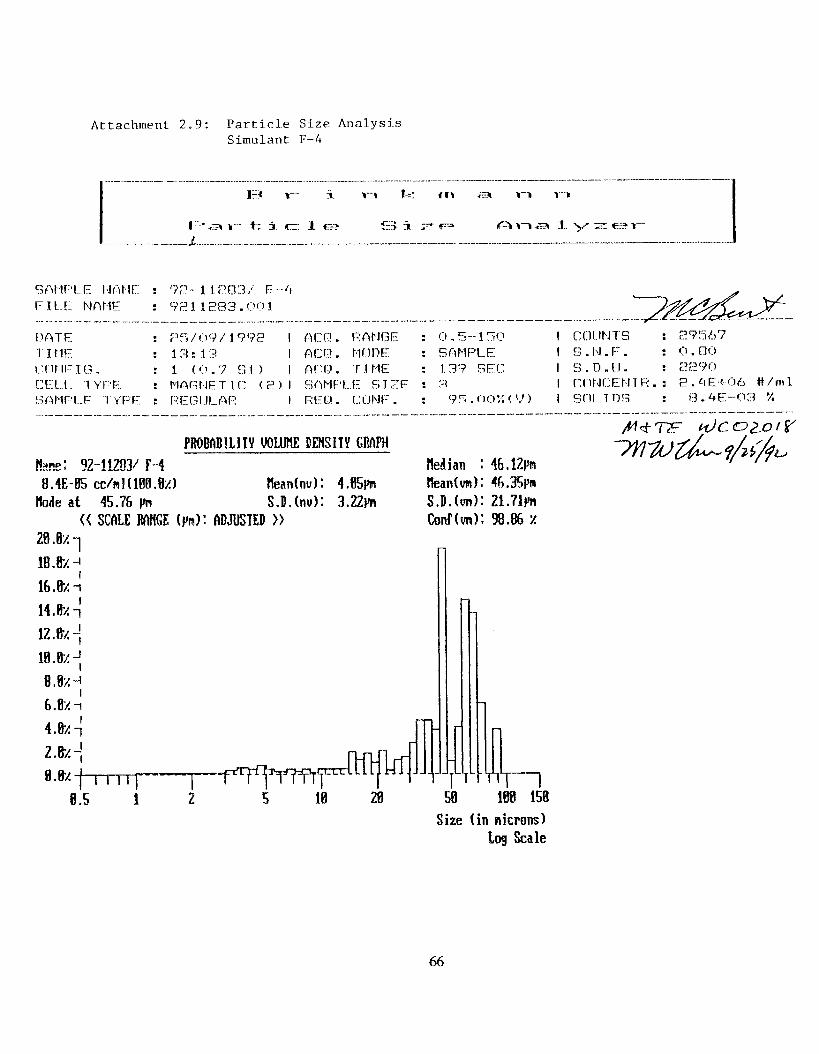
At tachmen t 2 . 9 : Particle S i z e Analysis Simulant F-4

PROBRBlLITY VOLUllE DENSITY GMPH

66

Attachment 2.10: Particle Size A n a l y s i s S imulan t F-5

m 1fM 158

Size ( i n aicrons) Log Scale

67

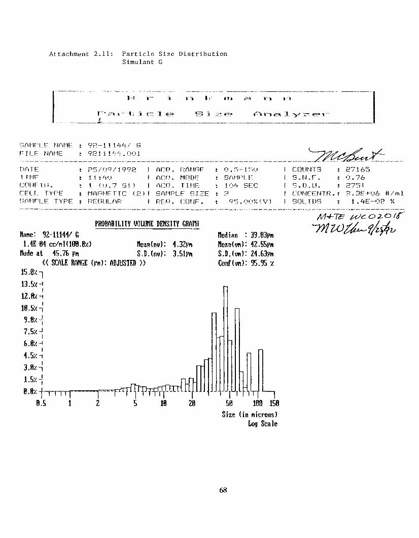
Attachment 2.11: Particle Size Distribution S imulan t G

n

8 .e2 - ~ ~ - ~ - ~ 8.5 I 2 5 18 20 50 100 158

Size ( i n nicrons) Log Scale

68

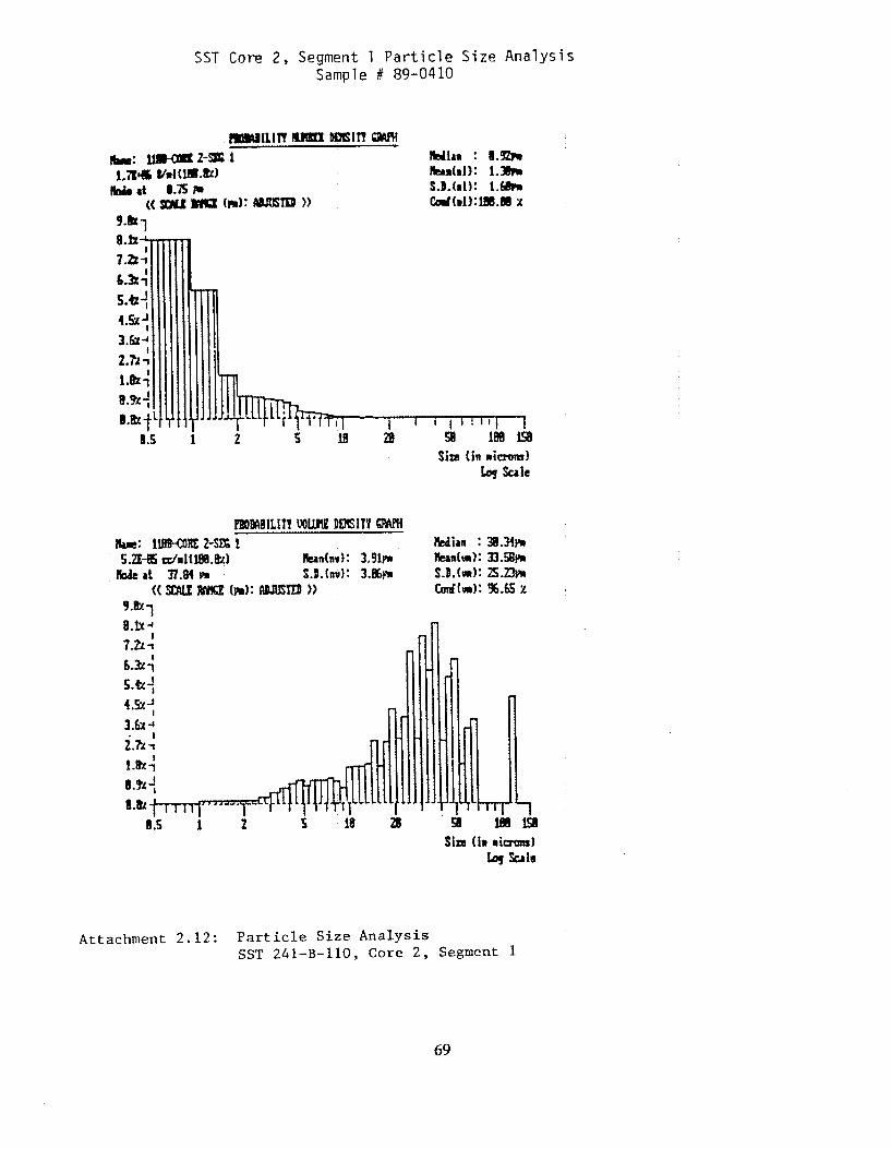
SST Core 2, Segment 1 P a r t i c l e S ize Analys is Sample # 89-0410

Sin (in riaanal h g kale

4.9;

2.rr 1 3.62 -4

I

8.S 1 2 ~ !

Attachment 2.12: Particle Size Analysis SST 241-B-110, Core 2, Segment 1

69

SSP Core 2 , Segment 2 P a r t i c l e S i z e A n a l y s i s Sample # 89-041 1

Sin! (in ricrons) log S a l e

6.h7 5.b -4

I 4.ki 4.22: 3.6.4: 3.Rq 2.h -4

1.Ri-l 1.8 1

I

I

1.5 1

Attachnent 2.13:

~ 5 l e a sa lee 158

Particle Size Analysis SST 241-B-110, Core 2, Segment 2

70

SST Core 2, Segment 4 Par t ic le Size Analysis Sample # 89-0423

Sire ( in n i t ram)

Ly Sule

Attachment 2.14: Particle Size Analysis SST 241-B-110, Core 2 , Segment 4

71

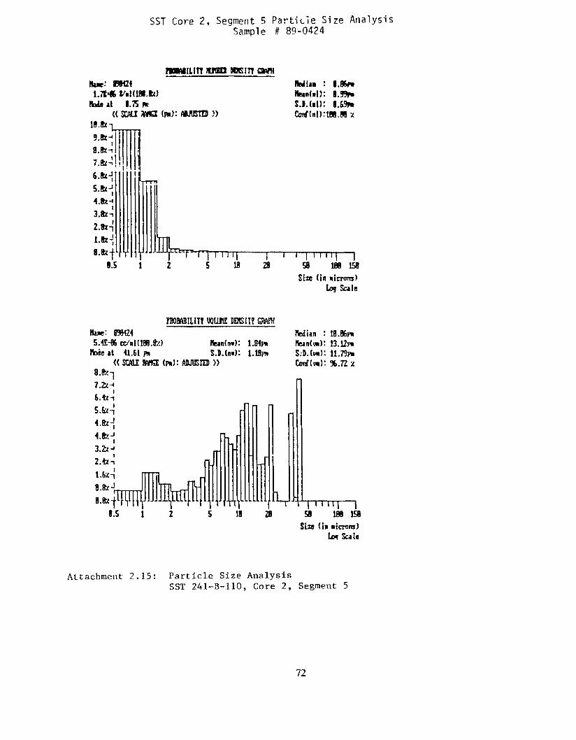
SST Core 2, Segment 5 P a r t i L i e S i z e A n a l y s i s Sample # 89-0424

2 5 i 18 I d

Attachment 2.15: Particle Size Analysis SST 241-B-110, Core 2, Segment 5

72

Attachment 3: Range of Constituents in SSTs (Based on the Analyses of 18 SSTs)

Ai Si Fe P Bi U Zr

NO,-

Ca Na NO,-

50:

0

Cr K

Pb %a Mn Ni Zn Cd Sr Ag B

cu Co

TOC

Mg

Range of Major Constituents in Sludge

I =meanvalue

I 1

I I 1 I T

10 20 30 % (Weight) of Total Dry Solids

40

Range of Minor Constituents in Sludge I

I ' , * 1 + = mean value

I

1 I I I 1 I 0.00 0.25 0.50 0.75 1.00 1.25 1.50 1.75

% (Weight) of Total Dry Solids

(EO Jones, NG Colton, and GR Bloom, "Hanford Single-Shell Tank Waste: Preliminary Pretreatment Testing of Simulated Waste," presented at the 7th Annual DOE Model Conference, Oak Ridge, TN, October, 1991)

73

APPENDLX B

Pressure Drop versus Flow Rate Curves for MVST Runs MVST 5 3,3A, 3B, and 3C and Hanford Singleshell Tank Siuiated Waste Runs H-1 through H-7, and

Tabulated Rheology Data for Hanford ShgIeShell Waste Runs H-1 through €3-7

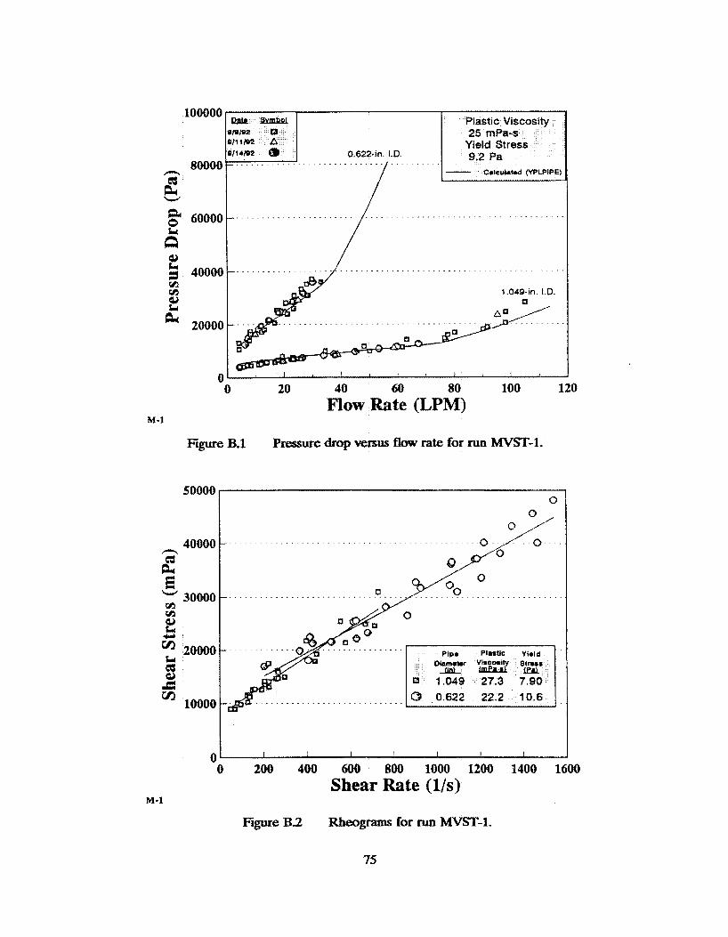
M-1

. . . . . . . . . . .......

1.049-in. 1.0.

0 20 40 60 80 100 120

Flow Rate (LPM)

Figure B.1 Pressure drop versus flow rate for run MVST-1.

50000

40000 h

&

3; 20000

3 * 10000

E - 30000 tn u2 Q) Lc

Lc

m a

., 0 200 400 600 800 1000 1200 1400 1600

Shear Rate (Us) m-i

Figure B2 Rheagrams for run MY=-1.

7s

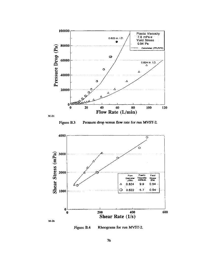
7.8 mPa-s Yield Stress 0.94 Pa

0 622-111. I.B.

100000

2 80000 L v

0 20 40 60 80 100 120 Flow Rate (L/min)

M-2b

Figure B 3 Pressure drop versus flow rate for run MVS-2

4000

h

8 3000 E

E 2000 3;

E! 3 1000

W

m m

L,

0 0

M-2b

0

pip. Plastic Yield Diameter Viscosity Strass llILLImPa-.lw

A 0.824 9.9 0.94

0 0.622 5.7 0.94

I I

200 400 Shear Rate (Us)

600

Figure B.4 Rheogams for MVS-2

76

100000

W

a

aa Lc 2 40000 m

Llr 20000

(I

M -3

. . . . . . . . . . . ......

0.824-in. I.D.

. . . . . . . . . . . . . . . . .

1.049-in. I.D.

I I I I

20 40 60 80 100 120 Flow Rate (Wmin)

Figure Bf Pressure drop versus flow rate for run MVST-3.

M -3

. .

200 400 600 800

Shear Rate (Us)

Figure B.6 Rheograms for run W S T - 3 .

80000 pc W

t a 60000

Plastic Viscosity 0.622-in. I.? I-::: Yield ,"a"., Stress

.. Calcutatad (YPLPIPE)

-

/ 0.624-in. I.D. /

n

E 6ooo- E3 W

m m E 4000-

Lc 3;

$ m 2000 s

1.049-in I D 20000

0 0 20 40 60 80 100 120

Flow Rate (L/min) M-39

Figure B.7 Pressure drop versus flow rate for m a MVST-3k

-

0 ' I I I 1

0 200 400 600 800 Shear Rate (Us)

M-3a

f igure B.8 Rheograms for run MVST-3A

78

. . . . . . . . . . . . .

. . . . . . . . . .

. . . . . . .

Flow Rate (L/min) M-3b

Figure B.9 Pressure drop versus flow rate for run MVST-3B.

10000

. . . . . . . 8000 -. . . . . . n

lz . . . .

B - 6000

2 VI 4000

............. - . . . . . . . m CA

.y

L . .

& VI . . . . . . . . . . . . 2000 -

I I I

0 200 400 600 800 Shear Rate (l/s)

0

M-3b

Figure B.10 Rheograms for run MVST-3B.

79

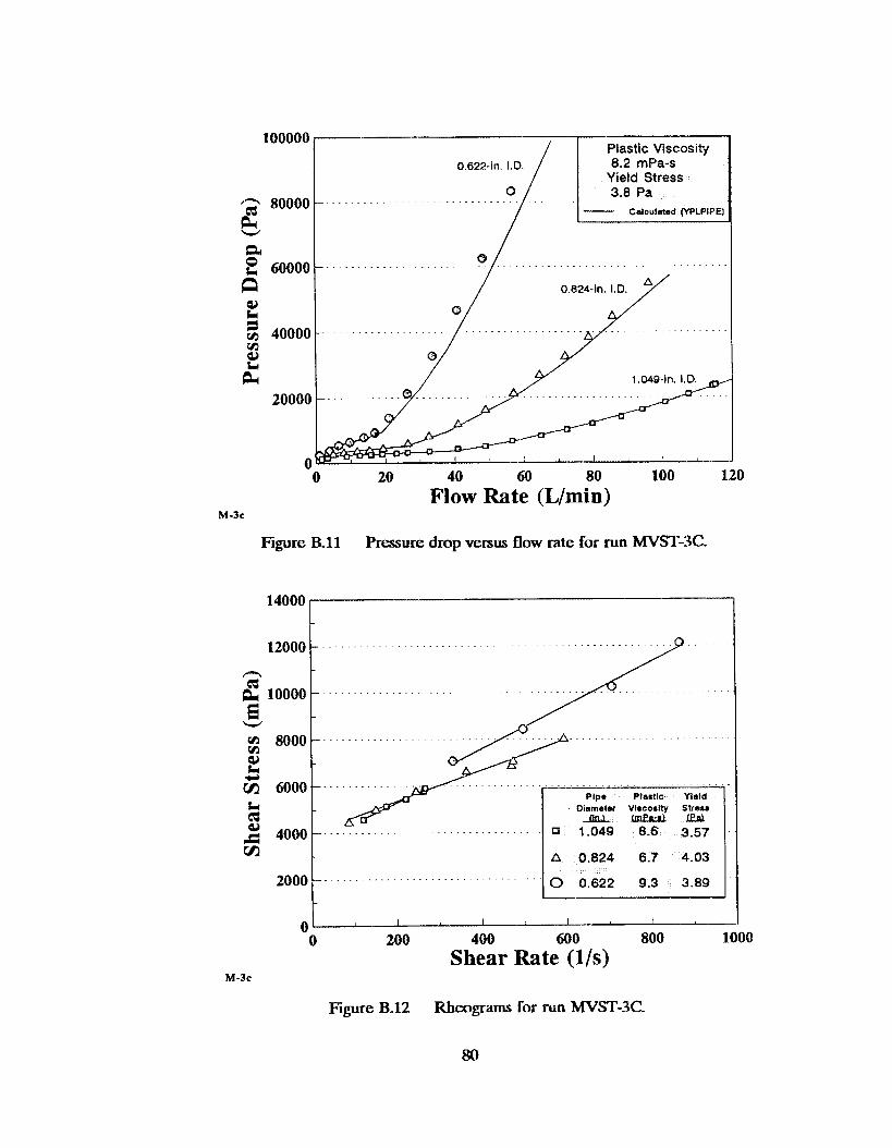
Plastic Viscosity

Yietd Stress

Caloulated (YPLPIPE) 2 80000 Plc W

60000 _ _ _ _ _ _ . . . . . . . . . .... . . . . t pc -7 0.824-in. I.D.

0 20 40 60 80 100 120

Flow Rate (L/min) M-3,

Figure B-11 Pressure drop versus flow rate for run MVST-3C.

14000

12000 F

4000 -

2000 . I I I I I I

0 200 400 600 800 1000 Shear Rate (l/s)

01

Figure B.12 Rheograms for run MVST-3C.

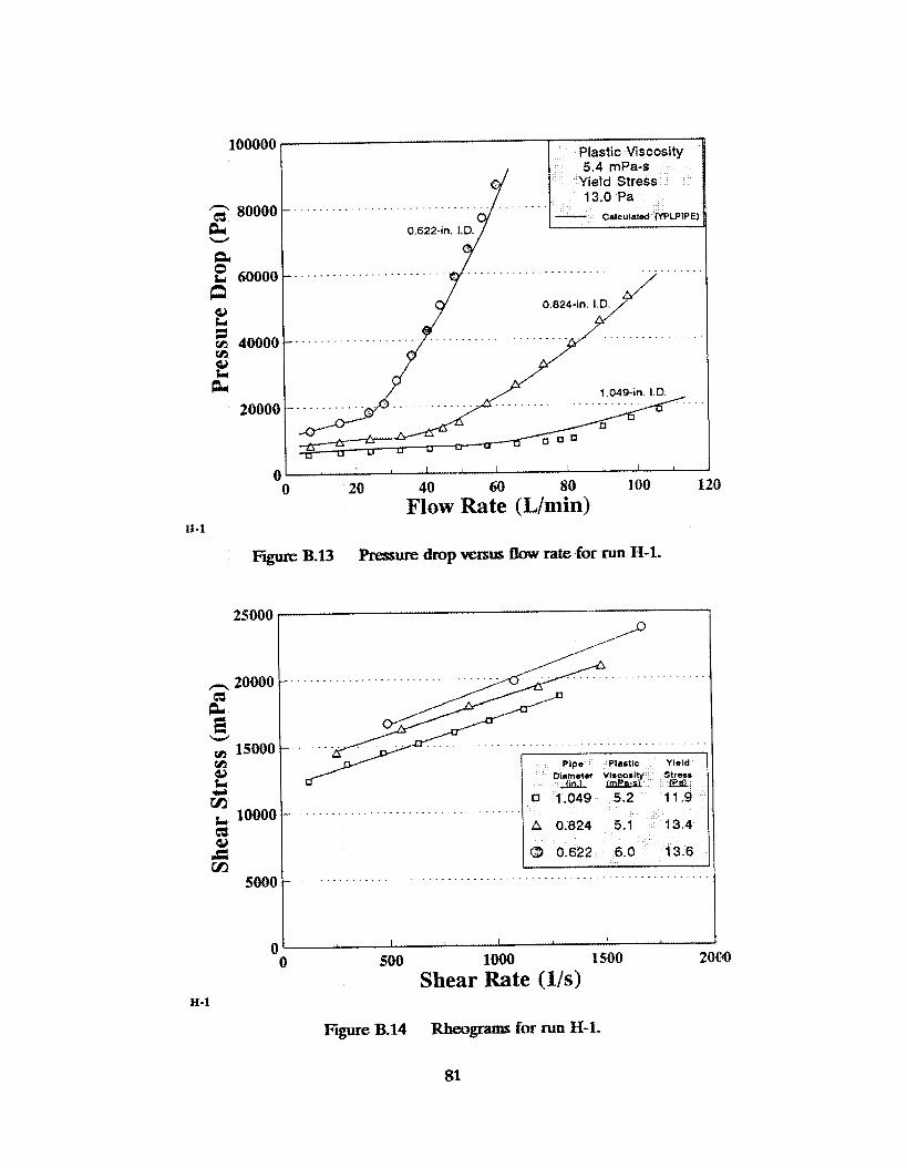
100000

2 40000 m Q)

r4: 20000

(

H-1

. . . . .

. . . . . . . . . . . . . . . . . . . . . . . . . . . . . . . . . . . . . . . . . . . . . . . . . . .

. . . . . . . . . . . . . . . . .

I I I I I

0 20 40 60 80 100 120

Flow Rate (L/min)

Egure B.13 Pressure drop versus flow rate for run H-1.

25000

c

. . . . . . . . . . . .

. . . . . . . . . . . . . . . . . . . . . . . . . . . . . . . . . . . . . . . . . . . . . . . . . . . . . . . . . . . . . .

I I I

500 loo0 1500 2000

Shear Rate (US)

81

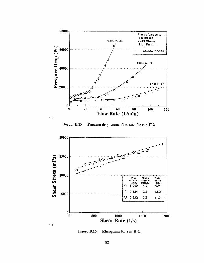
80000 r

I n 60000

W

0.622-in. 1.0.

P Plastic Viscosity 3.5 mPa-s

Yield Sfress 11.1 Pa

Calculsbd [YPLPIPE) -

H -2

n

0.82441-1, I.D.

I I I I

0 20 40 60 80 100 120 Flow Rate (Llmin)

Figure B.15 Pressure drop versus flow rate for run H-2,

20000

15000

10000

5000

0

Diameter Vlueoulty Stress m l n l & A L E A L

0 1.049 4.2 9.9

A 0.824 2.7 12-2

I I I

0 500 1000 1500 2000 Shear Rate (l/s)

H -2

Figure B.16 Rbeograrns for run H-2

82

80000 0.622-in. 1.0.

. . . . . . . n

& 6oooo W

E l 5 O O 0 - E

E 10000- ir;

3 5000-

W

cn cn

Li

H -3

. .

. . ...

I I I I I 1 0 20 40 60 80 100 120

Flow Rate (L/min)

Figure B.17 Pressure drop versus flow rate for run H-3.

20000 I 1

n

H-3

" 0 500 1000 1500 2000

Shear Rate (l/s)

Figure B.18 Rhagmms for run H-3.

83

Shea

r S

tres

s (m

Pa)

t4

VI 0

0

+

t4 0

0

01

0

0 0

CI 0 0

0

01 0

0

O0

ao

E

L

Pre

ssur

e D

rop

(Pa)

0

0

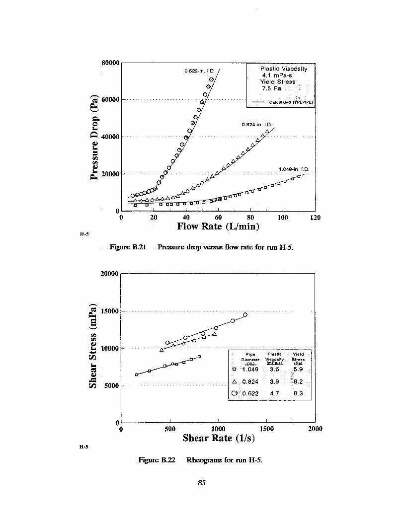
H-5

80000 0.622-tn. 1.0 Plastic Viscosity

4.1 mP Yield Si

- Calculntud fYPLPIPE) 2 6OOOO - .. ..

e plll

a

a 40000 4) Ll 1 v1 m Q)

v

0

. . . . . . . . . . . .

. . . . . . . . . . . . . . . . . . . . . . . . . . . . . . . . . . . . . . . . . . .

I I I I 1

0 20 40 60 80 100 120 Flow Rate (Wmin)

figure B21 Pressure drop versus Elow rate for NU H-5.

20000

15000

E

2 i 10000 3;

W

v1 m

Lc

= r/3 5ooc1

H-5

500 1000 1500 2000 Shear Rate (l/s)

Figure B-22 Rheograms for run H-5.

Plastic Viscosity 80000 I

Calculated (YPLPIPE)

0.622-117 1.D

n

pc a W

a 40000 /

H -6

. . . . . . . . . . . . . . . . . . . . . . . . .

Flow Rate (L/min)

Figwe B.23 Pressure drop versus flow rate for run H-6.

20000

A g 15000

El W

m m E 1000( Y m

i: rtl 5001

H-6

5 . . . . . . . . . . . . . . . . . . . . . . . . . . . . . . . . . . . . . . . . . . . . . . . . . . . . . . . . . . . .

8 0.622 4.4 7.9

Plastic Yield viscosity Stress hmislm

2.1 6.6

h 0.824 2.1 8.4

8 0.622 4.4 7.9

In 1.049

I I I I 500 1000 1500 2000

Shear Rate (l/s)

Figure B.24 Rheograms for run H-6.

86

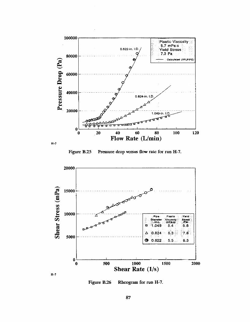
u-1

. . . . . . . . . . . . . . . . . . . . . . . . . . . . . . . . . . . . . . . . . . . . . . . . . . . . . .

. . . . . . . . . . . . . . . . . . . . . . . . . . . . . . . . . . . . .

100000

80000 n

& W

Q)

v1 tn

40000

E P w i 20000

. . . . . . . . . . . .

0.622-in. I.D. .9

0 20 40 60 80 100 120 Flow Rate (L/min)

figure €3.25 Pressure drop versus Bow rate for run H-7.

20000

h

15000

B W

r%l 5000

0

. . . . . . . . . . . . . . . . . . . . . . . . . . . . . . . . . . . . . . . . . /

........ . . . . . . . . . . . . . . . . . . . . .

0 500 1000 1500 2000

Shear Rate (Us ) H -7

figure B26 Rheogram for run H-7.

87

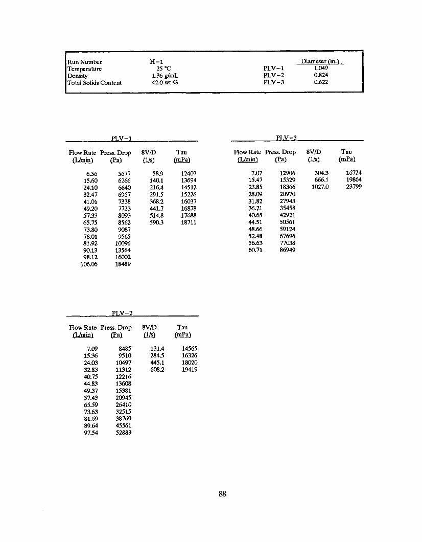
Run Number H-1 Temperature 25 "C

Total Solids Cantent Density 1.36 ghnL

42.0 wt %

Diameter (in.) p1v-1 1.049 p1v-2 0.824 PLV -3 0.622

I J

PLV-1

FlowRate Press.Drop 8VD Tau Q42!Z!(Pa) m (mUa)

656 15.60 24.10 32.47 41.01 49.20 57.33 65.75 73.80 78.01 81.92 90.13 98.12

106.06

5677 58.9 6266 140.1 6640 216.4 6967 2915 7338 -768.2 7723 441.7 8093 514.8 8562 590.3 9087 9565

10096 13564 16002 18489

12407 13694 14512 15226 16037 16878 17688 18711

FlowRate Press.Drop 8v/D Tau f2E! .kQma) m (mPa)

7.09 15-16 24.03 32.83 40.75 44.83 4937 57.43 6559 73.63 81.69 89.64 97.54

8485 131.4 14565 9510 2845 16326

10497 445.1 18020 11312 608.2 19419 12216 13608 15381 20945 26410 32515 38769 45561 52883

p1v-3

RowRate PresDrop SV/D Tau o m m @m

7.07 15.47 23.85 28.09 3 1.82 36.21 40.65 44.5 1 48.66 52.48 56.63 60.71

12906 304.3 16724 15329 666.1 19864 18% 1027.0 23799 20970 27943 35458 42921 50561 59124 67696 790-38 86949

88

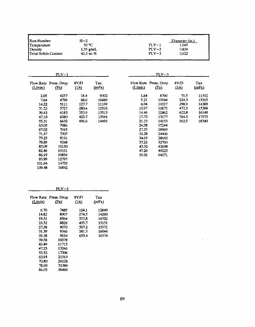
Run Number H-2 Temperature so "C Density 135 g/mL Total Solids Content 42.3 wt %

Diameter (in.) p1v-1 1.049 p1v-2 0.824 p1v-3 0.622

PLV-1 p1v-3

FlowRate P r e s . S . ~ 8VD w

205 7.64

14.22 3 1.22 39.42 47.19 5531 63.03 67.02 7157 75.25 78.89 83.09 82.46 86.19 93.99

101.64 109.48

CPa) a 4257 18.4 4799 68.6 5111 127.7 5727 280.4 6183 353.9 6380 423.7 6633 496.6 7086 7045 7307 8191 9248

10150 10101 10854 12797 14735 16842

Tau FlowRate Press.DnsD 8 V D Tau (mPa)

9302 10489 11169 12516 13513 13944 14495

PLV-2

FlowRate Press.Drop 8V/D Tau f!!&&OCPa) rn (mPa)

6.70 14.82 1931 23.52 27-78 3139 35-78 3958 43.49 47.23 5552 62.95 70.80 78.69 86.03

7485 124.1 12849 8.307 274.5 14260 8564 357.8 14702 8826 435.7 15151 9070 507.2 15571 9.346 581.5 16044 9654 655.4 16574

10078 11715 13246 17006 21313 26128 31384 36460

cumin)

1.64 5.21 6.94

10.97 14.46 17.75 21.19 2438 27.25 31.28 -34.65 37.21 4332 47.26 55.01

C9a)

8760 10044 11027 11875 12462 13177 14153 15244 18969 24406 28660 32760 42608 49223 64071

w 705

224.3 298.9 472.5 622.8 7645 912.5

(mPa)

11352 13015 14289 15388 16149 17075 18.340

89

I I Run Number H-3 Temperature 25 "C Density 1-36 ghnL Total Solids Content 42.4 wt %

Diameter (in.) p1v-1 1.049 p1v-2 0.824 p1v-3 0.622

I I

PLV-1

FlowRate Press.Drop 8VD Tau n / m i n ) ( P a ) @ J ( m P a )

13-78 19.93 28.20 36.73 44.97 53.06 61.21 69.09 76.45 8353 87.27 9480

102.01 109.40

4151 4245 178.9 9277 4616 253.2 10087 5179 329.8 11318 5599 403.8 12237 5%5 476.4 130% 6597 7668 9492

11302 12229 14280 16425 18694

PLV-2

FlowRate Pres.Drop 8V/D Tau n/min)m m

1222 15.48 19.78 27.98 28.25 3261 3655 4058 44.66 53.07 62.04 68.93 77.70 84.82 91.37

7251 7335 286.7 12591 7715 366.4 13244 8063 4443 13842 8573 5233 14718 9003 604.1 15455 9511

10689 12400 16687 21906 26528 32935 39016 44547

p1v-3

Tau FlowRate Press.Drop 8V/D G ! ! ! E i l ( P a ) llLsl (mPa)

8.69 1259 14.75 1751 19.64 22.00 25.36 28.19 31.18 .14.40 41.14 45.82 51.22 54.83

9509 314.4 12722 10337 542.0 13394 10813 635.1 14012 11441 754.0 14826 12177 845.7 15780 12966 947.6 16802 15119 19635 27977 28672 40221 49178 60768 68974

Run Number H-4 Temprature 25 "C Density 137 ghnL Total Solids Content 43.5 wt 96

Diameter {in.) p1v-1 1.049 p1v-2 0.824 p1v-3 0.622

FlowRate Press.Drap Q 4 E w C P a )

PLV-1 p1v-3

I Flow Rate Press. Drop Qfbi!! l Ipa)

8VD Tau w

8-76 4449 17.58 4890 26.54 5429 3429 5697 43.03 6183 51.15 6585 59.15 7047 67-30 7661 7131 8427 75.27 9497 78.80 10319 8286 11272 86.50 12271 9451 14359

101B 16604 11038 19013

8VD fLf9

75.0 1573 238.3 307.9 386.4 459.2 531.1

Tau (mPa)

9723 10687 11865 12450 13512 1439 1 15402

HowRate F'ress.Drop o m

8-36 8212 1331 8779 17.52 8805 21.98 9220 26.23 9647 30.26 10097 54.23 10580 38.59 11237 43.00 12739 46.82 14.368 51.08 16362 5537 18738 5920 21045 8233 38056 86.19 41278

154.9 246.6 3245 407.2 485.9 5m.s 634.1

Tau (mPa)

14098 14384 15115 15828 16560 17333 18163

0.87 8556 3.43 9479 4.26 10056 656 10700 8.89 11304

11-74 11972 14.98 1.3018 18.28 13976 22.50 15461 1439 13014 20.96 15093 23.47 16048 25.49 16974 27.12 18652 29.47 23420 3162 26819 34.34 31258 37.40 364% 41.40 43478 44.64 49293 47.38 55059 50-70 61297 5335 68281

375 11087 147.9 12283 1g3.5 130-30 2824 13865 382.7 14647 488.2 15514 6453 16869 787.3 18111 969.1 20035 619.6 16864 902.6 19558

1010.7 20795

91

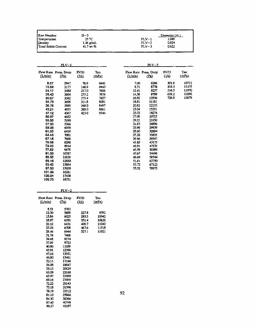
Run Number H-5 Diameter fin.)

Density 1.36 g/mL p1v-2 0.824 Total Solids Content 41.7 wt % p1v-3 0.622

Temperature 25 ‘C p1v-1 1.049

-

RowRate RwsDrop W/D Tau Flow Rate Press. Drop 8V/D Tau m u(slw - ( P a ) (IJsJW (Urnin’)

8.57 15.69 24.17 28.43 30.67 34.73 38.76 43.21 47.1 2 50.97 55.55 57.35 59.36 61.05 64.43 67.18 70.58 73.05 77.62 81.33 85.55 89.18 93.42 97.53

101.39 106.04 109.75

2947 3177 3480 3604 3582 3698 3888 4055 4367 4682 5190 5566 6058 6419 7081 7668 8288 8914 9879

10787 11836 12880 13884 15Q39 16281 17438 18731

76.9 140.9 217.0 255.2 275.4 311.8 348.0 388.0 423.0

6441 6943 7606 7876 7827 8081 8497 8861 9544

(Umin)

851 1230 15.84 18.97 2212 25.24 28.46 31.74 34.68 37.69 40.80 43.91. 47.16 49.m 53.11 56.08 59.13 63.09 65.97 69.14 l2.22 75.18 78.19 81.10 84.30 87.40 90.17

Flow Rate Press. Drop 8V/D Tau m m(mPa)

5782 5498 227.8 W82 6025 2935 10342 6191 351.4 10628 6431 m . 7 11040 6709 467.6 11518 6944 527.1 11921 7406 8274 9723

11039 12398 13951 15461 17166 18847 20629 23168 w389 27059 29143 313% 335 12 35866 38366 40749 43197

7.00 9.71

1241 1438 16.92 18.81 20.82 23.04 25.a 27.09 29.22 31.63 33.98 35.60 37.28 39.66 41.85 43.91 45.59 47.67 49.69 51.61 53.72 5552

92

8266 301.6 10711 8775 418.3 11375 9237 5345 11970 9799 619.2 12698

10556 72&8 13679 11181 12122 15351 18274 20725 23350 268% 29939 32884 35855 39547 43175 47276 m99 544% 58464 62750 67122 70975

I 1 Run Number H-6 Temperature SOT Density 1-36 g/mL Total Solids Content 427 wt %

Diameter (in.) * PLV-1 1 .w

p1v-2 0.824 p1v-3 0.622 I I I

PLV- 1

FlowRate Press.Drop c u m i n ) o

5.90 3125 9.18 3203

14.26 ,391 19-04 -3463 23.19 3617 27.24 3663 3153 3762 35.61 3871 39.60 4168 43.59 4215 47.60 4170 51-39 4356 55.41 4619 59.11 5273 8.17 6108 66.86 6825 70.98 7528 75.00 8302 78s sow 8273 rn 86.42 108 12 90.52 11744 94.41 12818

8V/D w

53.0 82.4

128-0 170.9 2118.2 244.6 283.1 319.7

Tau (mpa)

6829 7000 7411 7569 7905 8005 8222 8460

PLV-2

FlowRate pI.essDrop 8V/D Tau - ( p a ) M ( m p a l

656 1054 14.40 1831 21-34 24.10 27.11 30.19 33-38 36.42 3932 4226 45.36 48.48 5223 55.86 58.95 6297 66.77 70.73 75.01

5222 5490 5714 5918 6067 6204 6365 6616 6931 7999 a77

1Wa3 11733 13179 14994 16W 18701 21005 27450 25761 28646

121.6 1953 266.8 339.2 3953 446.4 5a23 5593

8965 9425 9809

10160 10415 10651 1092.6 11357

p1v-3

HowRate F’ress.Drop 8VD - ( P a ) rn

6.16 7550 m.3 8.86 8076 381.4

11.91 8594 512.9 13.94 8952 60a3 1J.74 9489 677.9 17.28 9881 744.3 19.25 10470 20.46 10931 2214 12Mx) 27.19 13853 24.86 15952 2750 18992 2931 21012 3136 27812 33.29 26488 3521 29204 3756 32758 3-53 35419 41.98 39456 43.44 41720 4535 44959

93

Tau (mPa)

9783 10465 11137 11601 12296 12804

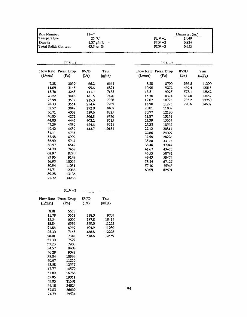
Run Number H-7 Temperature 25 "C Density 137 ghnL 9

Total Solids Content 435 wt %

Diameter (in.) p1v-1 1.049 p1v-2 0.824 p1v-3 0.622

PLV-1 p1v-3

FlowRate Press.Drop 8V/D Tau Flow Rate Press. Drop 8V/D Tau o m @I

738 11.09 15.78 20.22 27.98 2833 3252 36.71 40.85 44.80 47.29 49.42 51.11 53.48 56.99 60.97 64.70 68.97 72.96 76.95 80.94 84.71 89-28 92.72

3039 3145 3265 3418 3632 3654 3847 40-38 4272 4446 4539 4659 4735 4999 5737 6647 7467 8280 9149

10066 11051 12066 13136 14233

66.2 99.6

141.7 1815 2153 254.4 292.0 329.6 366.8 402.2 424.6 443.7

PLV-2

FlowRate Press.DroIp 8V/D @&nin) (PaJ fY.9

8.01 11.78 1554 18.84 21.86 25-30 28.01 31-30 33.23 -3457 -36.28 38.84 40.67 4358 47.77 51.89 55.85 59.85 64.10 67.83 71.79

5655 5652 2183 6066 287.8 6539 349.0 6949 404.9 7163 468.8 7316 518.8 7679 7960 8403 9092

10339 11256 12557 14579 16768 19051 21501 24024 26669 29534

(mPa)

6641 6874 7135 7470 79.38 7985 8407 882s 9336 9715 9921

10181

Tau (mPa)

9703 10414 11225 11930 122% 12559

94

Ivmin, 8.28

10.90 1331 1550 17.02 18.50 20.01 20.77 21.87 2739 2535 27.12 29.86 3258 35.68 38.46 41.67 4555 49.43 53.24 57.10 60.09

8790 3565 11390 9272 469.4 12015 9925 573.1 12862

10394 667.8 1.3469 1W73 733.2 13960 11273 796.6 14607 11807 12180 13151 15664 18562 20814 24079 28226 33178 37942 43426 50792 28474 67127 75948 82691

95

1. M. R. Ally 2. W. D. Arnold 3. P. L. Askew 4. T. J. Abraham 5. P. E. Arakawa 6. J. W. Autry 7. J. M. Begovich 8. J. T. Bell

9-13. J. B. Berry 14. M. D. Boring 15. C. H. Brown 16. C. H. Byers 17. C. Clark, Jr. 18. D. A. Conatser 19. A G. Croff

20-24. R. L. Cummins 25. S . J. Davidson 26. D. L Daugherty 27. S. M. DePaoli 28. J. R. DeVore 29. T. L. Donaldson 30. J. T. Etheridge 31. J. R. Forgy, Jr. 32. V. L. Fowler 33. C. E. Frye 34. H. R. Gaddis 35. S. B. Garland

ORNL/l%l- 12660

INTERNAL DISTRIBUTION

36. R. K- Genung 37. J. R. Hightower 38. R. D. Hunt

39-43. T. D. Hylton 44. L. L. Jacobs 45. L. L. Kaiser 46. C. M. Kendrick 47. T. E. Kent 48. J. R. Lawson 49. R. Macon 50. J. D. Maddox 51. C. P. Manrod 52. R. C. Mason 53. A J. Mattus 54. E. W. McDaniei 55. C. P. McGinnis 56. B. C. McClelIand 57. L. E. McNeese 58. R. C. Orrin 59. J. R. Parrott, Jr. 60. B. D. Patton 61. 1. J. Perona 62. J. G. Pruett 63. S. M. Robbinson 64. S. T. Rude11

65-69. E R. R u p ~ l

70. T. F. Scanlan 71. C. B. Scott 72. J. A. Setaro 73. R. 3. Shelton 74. J. L. Snyder 75. R. C. Stewart 76. L. E. Stratton 77. W. T. Thompson 78. J. R. Trabalka 79. J. R. Travis 80. M. W. Tu11 81. D. W. Turner 82. R. I. Van Hook 83. J. F. Walker 84. J. H. Wilson

85-89. E. L. Youngblood 90. Central Research

91. Document Reference Library

Sect ion 92-93. Laboratory Records

94. Laboratory Records,

95. ORWL Patent Section R.C.

EXTERNAL DISTRTBUTION

96. Office of Assistant Manager, Energy Research and Development, DBE-OR, P.O. Box 2001, Oak Ridge, TN 37831

97-98. Office of Scientific and Technical Information, P. 0. Box 62, Oak Ridge, TN 37831 99. Sherry Gibson, DOE Headquarters, 12800 Middlebrook Road, Germantown, MD 20874.

100. J. 0. Moore, Division of Waste Management and Technology Development, DOE-OR, P.O. Box 2001, Oak Ridge, TN 37831

101. Dr. R. W. Hanks, Slurry Transport Consultant, 495 East 1010 South, Orem, Utah 84058. 102. M. R. Elmore, Pacific Northwest Laboratories, Battelle Boulevard, P.O. Box W, Richland,

WA 99352 103. N. C. Colton, Pacific Northwest Laboratories, Battelle Boulevard, P.O. Box 9 9 , Richland,

WA 99352

96

104. P. A Scott, Pacific Northwest Laboratories, Battelle Boulevard, P.O. Box 999, Richland, WA 99352

105. Roger L. Gilchrist, Manager, UST-ID, Westinghouse Hanford Company, P.0 . Box 1970, MSIN: L5-63, Richland, WA 99352

106. J. k Bamberger, Pacific Northwest Laboratories, Battelle Boulevard, P.O. Box 999, Richland, WA 99352

107. E. 0. Jones, Pacific Northwest Laboratories, Battelle Boulevard, P.O. Box 999, Richland, WA 99352

108. Dr. Inn Choi, Pacific Northwest Laboratories, Battelle Boulevard, P.O. Box 999, Richland, WA 99352

109. Mark A. Schiffhauer, West Valley Nuclear Services Co., Inc., P.O. Box 191, West Valley,

110. Dale Waters, Westinghouse Manford Company, P.O. Box 1970, MS S4-58, Richland,

111. Stephen D. Riesenweber, Westinghouse Hanford Company, RI-30, P.0 Box 1970, Richland

112. Brian Koons, Kaiser Engineers, 1200 Jadwin Avenue, MS E6-21, Richland, WA 99352 113. Robert E Eggers, Westinghouse Hanford Company, Retrieval Development, P.O. Box 1970,

MSIN S4-54, Richland, WA 99352 114. Walter Knecht, Westinghouse Hanford Company, P.O. Box 1970, MISN H0-34, Richland,

WA 99352 115. Dr. H. K Hepworth, Box 15600, Northern Arizona University, Flagstaff, AZ

NY 14171-0191.

WA 99352

WA 99352

86011-1560