Fluid acceleration effects on suspended sediment transport in the

Fluid acceleration effects on suspended sediment transport in the

swash zone

J. A. Puleo, K. T. Holland, and N. G. PlantNaval Research Laboratory, Stennis Space Center, Mississippi, USA

D. N. Slinn and D. M. Hanes1

Civil and Coastal Engineering Department, University of Florida, Gainesville, Florida, USA

Received 1 May 2003; revised 28 July 2003; accepted 3 September 2003; published 13 November 2003.

[1] Suspended sediment concentrations and fluid velocities measured in the swash zoneof a high-energy steep beach were used to investigate the importance of fluidaccelerations to suspended sediment transport. Swash flow acceleration was nearlyconstant at about one-half downslope gravitational acceleration with two importantexceptions. We observed strong, short-lived periods of accelerating uprush at thebeginning of the swash cycle and decelerating backwash at the end of the swash cycle(magnitudes of both approximately twice that of the expected downslope gravitationalacceleration). Interestingly, spikes in suspended load followed the anomalies inacceleration in a way that was not apparent from the nearly symmetric (in magnitude)ensemble averaged velocity time series. Suspended load values were largest duringaccelerating uprush associated with the shoreward propagating turbulent bore or swashfront. During backwash, suspended loads were generally not as large. Correspondingly,suspended sediment transport rates obtained from the sediment concentration andvelocity measurements showed best comparisons with a modified sediment transportmodel that includes a physical mechanism for enhancing transport rates due to flowacceleration. The modified sediment transport model reduced the overall root-meansquare prediction error by up to 35% and shifted the predicted peak in uprush sedimenttransport rate earlier in the swash cycle, resulting in a better fit to the observations.These findings suggest that the inclusion of the acceleration term may account forphysical mechanisms that include bore turbulence and horizontal pressure gradientstypically associated with the accelerating portion of uprush. INDEX TERMS: 4546

Oceanography: Physical: Nearshore processes; 4558 Oceanography: Physical: Sediment transport; 3020

Marine Geology and Geophysics: Littoral processes; KEYWORDS: uprush, swash zone bore, turbulence,

pressure gradient

Citation: Puleo, J. A., K. T. Holland, N. G. Plant, D. N. Slinn, and D. M. Hanes, Fluid acceleration effects on suspended sediment

transport in the swash zone, J. Geophys. Res., 108(C11), 3350, doi:10.1029/2003JC001943, 2003.

1. Introduction

[2] The swash zone is one of the most scientificallychallenging oceanic environments for describing sedimenttransport. Here, uprush and backwash motions mobilizeand transport large quantities of sediment compared toother regions [e.g., Beach and Sternberg, 1991; Hughes etal., 1997; Masselink and Hughes, 1998; Butt and Russell,1999; Osborne and Rooker, 1999 and Puleo et al., 2000].Gradients in the relatively small time-integrated transportdrive morphological change. In order to predict changesin beach morphology, an understanding of the physical

processes is needed to develop an accurate mathematicaldescription of sediment transport mechanisms in theswash zone.[3] Sediment transport in the swash zone has generally

been described with an energetics-type formulation origi-nally derived by Bagnold [1966] for steady unidirectionalflows and later adapted by Bowen [1980] and Bailard[1981] (hereinafter referred to as B3 models) for time-dependent flows and used in several studies [e.g., Hardistyet al., 1984; Hughes et al., 1997; Masselink and Hughes,1998; Puleo et al., 2000]. Although the range of observa-tions supporting these descriptions in the swash zone issomewhat limited, B3-type relationships have occasionallyshown some significant correlation between predicted andmeasured sediment transport rates [e.g., Masselink andHughes, 1998]. In addition, several studies have modifiedthe original B3 equations in the hope of increasing the

JOURNAL OF GEOPHYSICAL RESEARCH, VOL. 108, NO. C11, 3350, doi:10.1029/2003JC001943, 2003

1Also at U.S. Geological Survey Pacific Science Center, Santa Cruz,California, USA.

Copyright 2003 by the American Geophysical Union.0148-0227/03/2003JC001943$09.00

14 - 1

predictive skill at matching measurements. For instance,Puleo and Holland [2001] and Butt et al. [2001] havesuggested that the friction coefficient, f, varies betweenuprush and backwash and may even be a function of waterdepth. Since B3 models depend linearly on f, inclusion ofthis uprush-backwash variation could lead to improvementof sediment transport predictions either directly or indirectlyby accounting for unrelated physical processes.[4] The B3 type models rely on velocity moments and

hence do not explicitly account for flow unsteadiness thathas been shown to affect boundary layer structure andhence energy dissipation at the bed. An example wasgiven by King [1991] who showed that the boundary layerdevelopment is slowed in an accelerating flow, implyingthe thickness is less than that for a steady flow (furtherdescribed by Nielsen [1992]). The delayed development iseasily understood for a laminar flow where rapid velocitiesmay remain closer to the bed than in steady flow therebyincreasing the bed shear stress. This explanation is lessclear in a fully turbulent boundary layer where moremixing is likely to occur. Also, there is a phase lagbetween the free stream velocity and that in the boundarylayer. These unsteady boundary layer effects are notincorporated into the B3 models, even though they appearto have a significant influence on sediment transport [e.g.,Hanes and Huntley, 1986; Jaffe and Rubin, 1996]. Forinstance, Drake and Calantoni [2001] adapted a sheet flowmodel and added an extra term to the B3 bed load formulato account for acceleration effects (manifested throughhorizontal pressure gradients). Their numerical resultsshowed that the inclusion of acceleration effects signifi-cantly improved the skill of the sediment transport model.Fluid accelerations have also been related to sandbarmorphology [Elgar et al., 2001; Hoefel and Elgar, 2003]where it was shown that the peak in acceleration skewnessof surf zone flows was well correlated to onshore sandbarmotion. Admiraal et al. [2000] developed relationshipsbased on fluid accelerations and sediment response topredict the phase lag between maximum shear stress andpeak suspended sediment concentrations from laboratorymeasurements in a flume.[5] While several studies have addressed the effect of

fluid acceleration either from a theoretical viewpoint or forthe surf zone, fewer studies have applied these concepts tothe swash zone. Nielsen [2002] adopted the Meyer-Peterand Muller [1948] sediment transport model for swash byincluding a phase shift in the shear stress term. This phaseshift accounts for greater bed shear stresses for a givenvelocity during accelerating flow. In the swash zone, this ismost important to the accelerating portion of the uprushwhere peak velocities are higher and sediment tends to bemore concentrated than during backwash [e.g., Butt andRussell, 1999; Puleo et al., 2000]. In fact, Butt and Russell[1999] used field data to show that sediment suspensionevents coincided with periods of large onshore-directedfluid acceleration.[6] The primary aim of this study is to describe the link

between fluid acceleration and sediment transport in theswash zone, using field observations from a natural beach.The secondary aim is to use the new understanding of swashzone sediment transport to make a modification to the B3model and to test this modification. Section 2 describes the

expected fluid motions based on idealized models. TheB3-type sediment transport equation and the modificationcaused by including acceleration are presented in section 3.Section 4 briefly describes the field set up and datacollected. Observations of suspended loads in velocity-acceleration space and comparisons between observationsand model predictions are given in section 5. Discussionand conclusions are given in sections 6 and 7, respectively.

2. Idealized Swash Motions and SedimentTransport

[7] Before developing the acceleration-based modifica-tion for the swash zone application of the Bailard model, itis important to understand the context to which thisacceleration may play a role in swash zone suspendedsediment transport. Technically, the swash motion beginsafter bore collapse into very shallow water [O(mm - cm)]or exposed (possibly wetted) bed. The inertia of theshoaling wave and the pressure force from the collapseaccelerate the mass of water up the beach face. Toward theend of the backwash the seaward directed flow collideswith the next incident bore (decelerates) leading to theensuing swash event.[8] Frictional ballistic motion often applied to describe

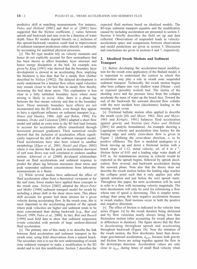
the swash cycle [Ho and Meyer, 1962; Shen and Meyer,1963 and Kirkgoz, 1981] balances fluid accelerationagainst gravity and friction (see Puleo and Holland[2001] for analytic formulation). An example showing aLagrangian velocity and acceleration time history for theleading edge and solely cross-shore flow is given inFigure 1 (defining the cross-shore direction, x, to bepositive offshore). The flow is modeled analogous to ablock moving up and down a frictional incline with abeach slope of 1:12, initial velocity, u0, of 4 m s�1,friction factor of 0.01 and a leading edge water depth of0.05 m. An instantaneous increase in velocity would beexpected as the uprush begins, followed by uprush decel-eration, flow reversal, and backwash acceleration duringthe seaward phase. Note also that the theory does notdescribe the swash motion before the leading edge reachesthe collapse point such that it only applies just afteruprush initiation and just before the next uprush starts.Throughout this paper, the term acceleration will be usedto refer to a flow with increasing velocity magnitude. Theterm deceleration will only be used for referencing a flowwhose rate of speed is decreasing. This is simpler termi-nology than using the term negative acceleration becausein swash studies, fluid motions occur in both the positiveand negative directions.[9] The effect of friction is indicated in the velocity time

series (Figure 1a) by the swash duration being shortenedand by flow velocities nearly always being less thanfrictionless motion (after accounting for swash phase dueto differences in duration). The figure shows that the flowis decelerating throughout uprush and acceleratingthroughout backwash (Figure 1b). Near the initiation ofthe swash motion, the flow decelerates faster than down-slope gravitational acceleration, agrav, because both gravityand friction forces are acting together against the flow inthe downslope direction. Acceleration values are onlyclose to agrav during times of small fluid velocity when

14 - 2 PULEO ET AL.: SWASH ACCELERATION AND SEDIMENT FLUX

the friction force is also small. After flow reversal, theacceleration is less than agrav because friction and gravityforces are opposing each other. In short, the simplefrictional theory for Lagrangian swash edge motion pre-dicts a decelerating uprush and accelerating backwashduring their respective cycles.[10] While the Lagrangian description of leading edge

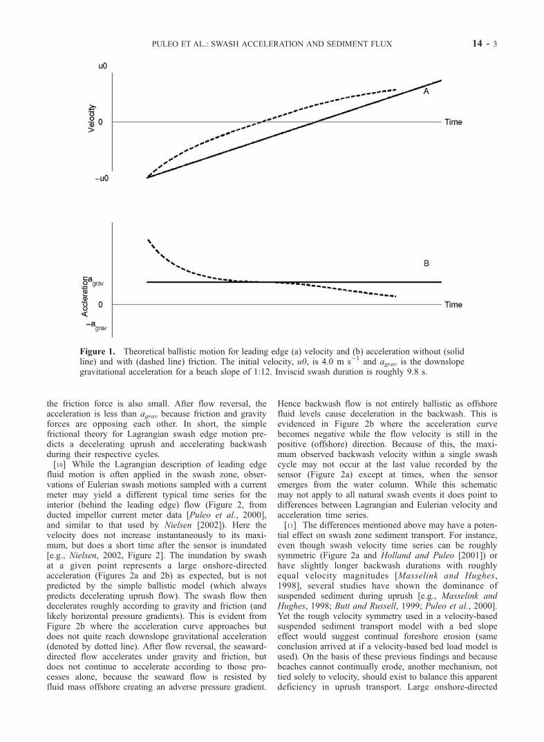
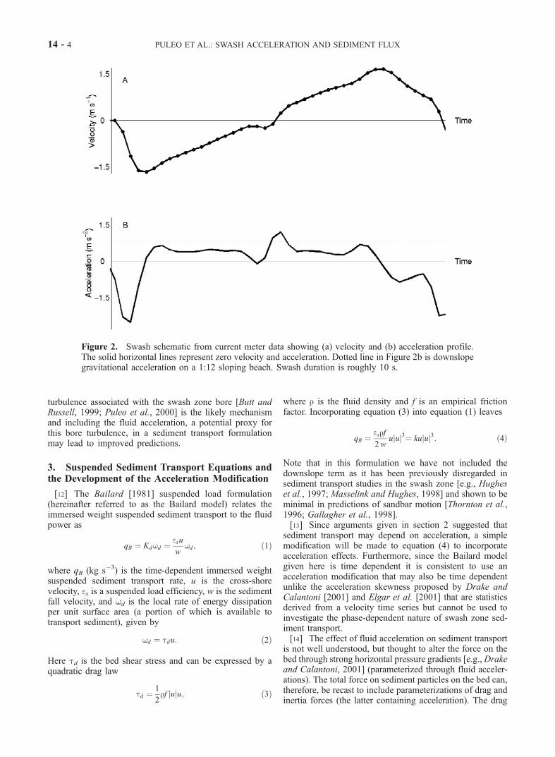
fluid motion is often applied in the swash zone, obser-vations of Eulerian swash motions sampled with a currentmeter may yield a different typical time series for theinterior (behind the leading edge) flow (Figure 2, fromducted impellor current meter data [Puleo et al., 2000],and similar to that used by Nielsen [2002]). Here thevelocity does not increase instantaneously to its maxi-mum, but does a short time after the sensor is inundated[e.g., Nielsen, 2002, Figure 2]. The inundation by swashat a given point represents a large onshore-directedacceleration (Figures 2a and 2b) as expected, but is notpredicted by the simple ballistic model (which alwayspredicts decelerating uprush flow). The swash flow thendecelerates roughly according to gravity and friction (andlikely horizontal pressure gradients). This is evident fromFigure 2b where the acceleration curve approaches butdoes not quite reach downslope gravitational acceleration(denoted by dotted line). After flow reversal, the seaward-directed flow accelerates under gravity and friction, butdoes not continue to accelerate according to those pro-cesses alone, because the seaward flow is resisted byfluid mass offshore creating an adverse pressure gradient.

Hence backwash flow is not entirely ballistic as offshorefluid levels cause deceleration in the backwash. This isevidenced in Figure 2b where the acceleration curvebecomes negative while the flow velocity is still in thepositive (offshore) direction. Because of this, the maxi-mum observed backwash velocity within a single swashcycle may not occur at the last value recorded by thesensor (Figure 2a) except at times, when the sensoremerges from the water column. While this schematicmay not apply to all natural swash events it does point todifferences between Lagrangian and Eulerian velocity andacceleration time series.[11] The differences mentioned above may have a poten-

tial effect on swash zone sediment transport. For instance,even though swash velocity time series can be roughlysymmetric (Figure 2a and Holland and Puleo [2001]) orhave slightly longer backwash durations with roughlyequal velocity magnitudes [Masselink and Hughes,1998], several studies have shown the dominance ofsuspended sediment during uprush [e.g., Masselink andHughes, 1998; Butt and Russell, 1999; Puleo et al., 2000].Yet the rough velocity symmetry used in a velocity-basedsuspended sediment transport model with a bed slopeeffect would suggest continual foreshore erosion (sameconclusion arrived at if a velocity-based bed load model isused). On the basis of these previous findings and becausebeaches cannot continually erode, another mechanism, nottied solely to velocity, should exist to balance this apparentdeficiency in uprush transport. Large onshore-directed

Figure 1. Theoretical ballistic motion for leading edge (a) velocity and (b) acceleration without (solidline) and with (dashed line) friction. The initial velocity, u0, is 4.0 m s�1 and agrav is the downslopegravitational acceleration for a beach slope of 1:12. Inviscid swash duration is roughly 9.8 s.

PULEO ET AL.: SWASH ACCELERATION AND SEDIMENT FLUX 14 - 3

turbulence associated with the swash zone bore [Butt andRussell, 1999; Puleo et al., 2000] is the likely mechanismand including the fluid acceleration, a potential proxy forthis bore turbulence, in a sediment transport formulationmay lead to improved predictions.

3. Suspended Sediment Transport Equations andthe Development of the Acceleration Modification

[12] The Bailard [1981] suspended load formulation(hereinafter referred to as the Bailard model) relates theimmersed weight suspended sediment transport to the fluidpower as

qB ¼ Kdwd ¼esuw

wd ; ð1Þ

where qB (kg s�3) is the time-dependent immersed weightsuspended sediment transport rate, u is the cross-shorevelocity, es is a suspended load efficiency, w is the sedimentfall velocity, and wd is the local rate of energy dissipationper unit surface area (a portion of which is available totransport sediment), given by

wd ¼ tdu: ð2Þ

Here td is the bed shear stress and can be expressed by aquadratic drag law

td ¼1

2rf uj ju; ð3Þ

where r is the fluid density and f is an empirical frictionfactor. Incorporating equation (3) into equation (1) leaves

qB ¼ esrf2w

u uj j3¼ ku uj j3: ð4Þ

Note that in this formulation we have not included thedownslope term as it has been previously disregarded insediment transport studies in the swash zone [e.g., Hugheset al., 1997; Masselink and Hughes, 1998] and shown to beminimal in predictions of sandbar motion [Thornton et al.,1996; Gallagher et al., 1998].[13] Since arguments given in section 2 suggested that

sediment transport may depend on acceleration, a simplemodification will be made to equation (4) to incorporateacceleration effects. Furthermore, since the Bailard modelgiven here is time dependent it is consistent to use anacceleration modification that may also be time dependentunlike the acceleration skewness proposed by Drake andCalantoni [2001] and Elgar et al. [2001] that are statisticsderived from a velocity time series but cannot be used toinvestigate the phase-dependent nature of swash zone sed-iment transport.[14] The effect of fluid acceleration on sediment transport

is not well understood, but thought to alter the force on thebed through strong horizontal pressure gradients [e.g.,Drakeand Calantoni, 2001] (parameterized through fluid acceler-ations). The total force on sediment particles on the bed can,therefore, be recast to include parameterizations of drag andinertia forces (the latter containing acceleration). The drag

Figure 2. Swash schematic from current meter data showing (a) velocity and (b) acceleration profile.The solid horizontal lines represent zero velocity and acceleration. Dotted line in Figure 2b is downslopegravitational acceleration on a 1:12 sloping beach. Swash duration is roughly 10 s.


force on a sand grain and that extrapolated to the bed are bothgiven through a quadratic drag law. In a crude manner, wealso assume the inertial forces on a sand grain can besimilarly extrapolated to the bed yielding a combined force as

F ¼ Fd þ Fp ¼1

2rf uj juAþ rVkma; ð5Þ

where A is the bed surface area, V is the volume, a is the localfluid acceleration, and km is a constant coefficient. Theconvective acceleration, normally included in the inertiaforce, has not, to our knowledge, been studied in the swashzone, but future work may show its importance. It is excludedin this formulation since field measurements were obtainedfrom only a single location in the cross-shore (see section 4).Furthermore, particle intergranular forces normally includedin sediment transport models that operate at the particle scaleare not included here. The intent is to use a simple approachguided by some physical justification to determine the formof the acceleration term for the ‘‘macro’’ scale affect ofacceleration on sediment transport akin to the drag-law-driven energetics approach that is similarly focused onpredicting bulk sediment transport rather than grain-to-graininteractions and individual particle motions. If one wishes,the acceleration modification in equation (5) can be viewedsimilarly to the pressure gradient force extension used in theDrake and Calantoni [2001] model, but for instantaneousrather than time averaged transport predictions.[15] The total shear stress is then given by the total force

per unit area of bed as

t ¼ 1

2rf uj juþ rkmda; ð6Þ

whereupon division by the surface area, A, a vertical lengthscale, d, is needed. If the length scale is assumed to beconstant, then the logical choice for the length scale whenapplied to a single grain is the grain diameter. It is not clear,however, that the grain diameter is the appropriate lengthscale in this formulation for shear stress and hence it shouldnot be assumed that the inertia force is negligible whenapplied to the bed. Regardless, a constant length scalewould become incorporated into the leading coefficient andwould not need to be specified a priori. If, on the otherhand, one assumes that the acceleration in the swash zone islargely associated with the turbulent leading edge and bore[Butt and Russell, 1999], then a logical choice for the lengthscale would be the water depth since the turbulence is ableto extend from the water surface to the bed [Petti andLongo, 2001, Cowen et al., 2003]. For the time being, themodel will, for simplicity, include the length scale in theleading coefficient (assumes a constant value). Variationsarising from using the time-dependent water depth,however, will be mentioned in the results section.[16] Using equation (6) for the bed shear stress, a new

formulation for suspended sediment transport becomes

qpred ¼ kbu uj j3þka uj j2a; ð7Þ

where subscripts b and a represent coefficients for the Bailardmodel and the added acceleration effect, respectively.Throughout this paper, equation (7) will be referred to asthe modified model. Transport relationships like equation (7)

are often utilized in a time-averaged form such that atransport rate is determined per swash cycle or for a length oftime series. Time averaging erases all phase information. Inthis study, we are interested in the phase-dependent nature ofsediment transport throughout a swash cycle and will useensemble averages of swash events instead.

4. Field Study

[17] Data were collected at Gleneden Beach, Oregon, inFebruary 1994. This beach is intermediate to steep with aforeshore beach slope of roughly 1:12 and a median grainsize of 0.44 mm. Complete details of the data collection,reduction, and experimental setup are given by Puleo et al.[2000]. Briefly, two ducted impellor current meters (initially4 and 8 cm above bed), a pressure sensor (initially at bedlevel), and a fiber optic backscatter system (FOBS) tomeasure suspended sediment concentrations (penetratesthe bed so that bed level and suspension concentration towithin 1 cm of the bed can be obtained) were deployed atthree locations on the foreshore separated by 5 m in thecross-shore direction.[18] Data used in this study were obtained from the most

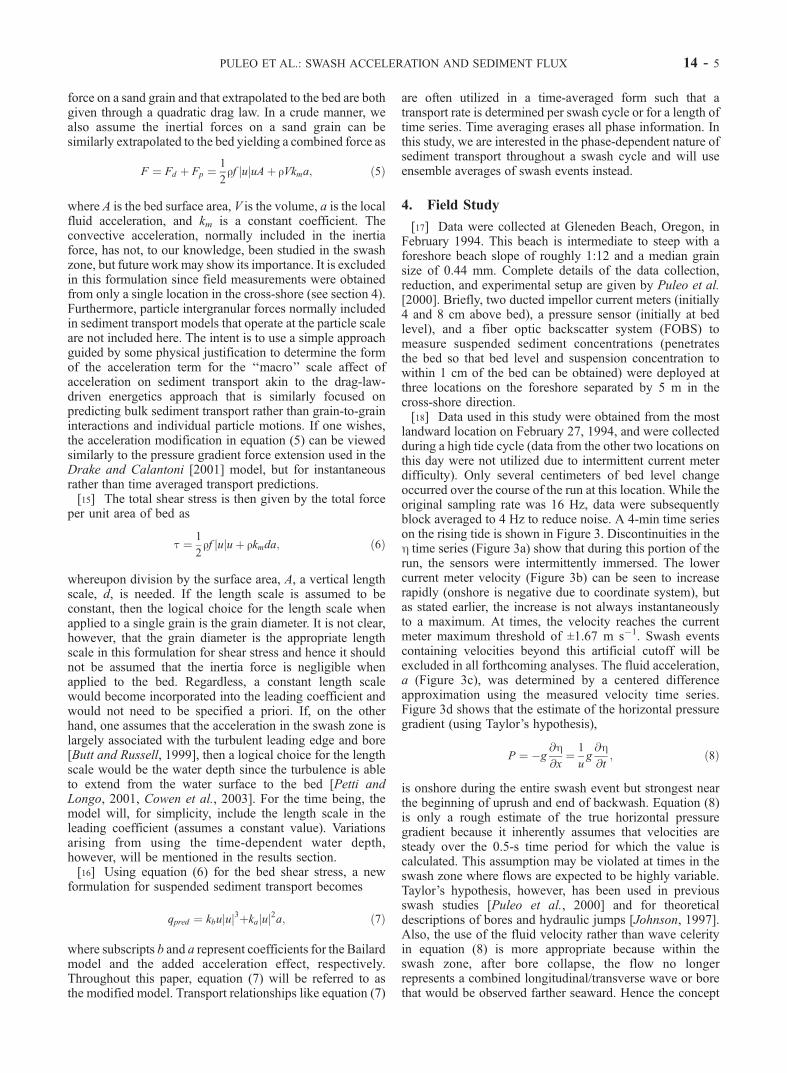
landward location on February 27, 1994, and were collectedduring a high tide cycle (data from the other two locations onthis day were not utilized due to intermittent current meterdifficulty). Only several centimeters of bed level changeoccurred over the course of the run at this location. While theoriginal sampling rate was 16 Hz, data were subsequentlyblock averaged to 4 Hz to reduce noise. A 4-min time serieson the rising tide is shown in Figure 3. Discontinuities in theh time series (Figure 3a) show that during this portion of therun, the sensors were intermittently immersed. The lowercurrent meter velocity (Figure 3b) can be seen to increaserapidly (onshore is negative due to coordinate system), butas stated earlier, the increase is not always instantaneouslyto a maximum. At times, the velocity reaches the currentmeter maximum threshold of ±1.67 m s�1. Swash eventscontaining velocities beyond this artificial cutoff will beexcluded in all forthcoming analyses. The fluid acceleration,a (Figure 3c), was determined by a centered differenceapproximation using the measured velocity time series.Figure 3d shows that the estimate of the horizontal pressuregradient (using Taylor’s hypothesis),

P ¼ �g@h@x

¼ 1

ug@h@t

; ð8Þ

is onshore during the entire swash event but strongest nearthe beginning of uprush and end of backwash. Equation (8)is only a rough estimate of the true horizontal pressuregradient because it inherently assumes that velocities aresteady over the 0.5-s time period for which the value iscalculated. This assumption may be violated at times in theswash zone where flows are expected to be highly variable.Taylor’s hypothesis, however, has been used in previousswash studies [Puleo et al., 2000] and for theoreticaldescriptions of bores and hydraulic jumps [Johnson, 1997].Also, the use of the fluid velocity rather than wave celerityin equation (8) is more appropriate because within theswash zone, after bore collapse, the flow no longerrepresents a combined longitudinal/transverse wave or borethat would be observed farther seaward. Hence the concept


of wave celerity for true swash flows is no longer applicableand the use of u is more appropriate.[19] The correspondence in Figures 3c and 3d imply that

the fluid acceleration may also serve as a surrogate for thepressure gradient estimate. Suspension pulses tend to occurduring sudden onshore-directed acceleration events as theswash reaches the sensors and during decelerating back-wash. Individual suspension pulses (Figures 3e–3j) can beseen with the passing of each swash event. The suspensionpulses extend at least 10 cm into the water column andlikely higher for some swash events. The suspension dataindicate that more sediment is generally carried as sus-pended load during the uprush than during the backwash asevidenced by the often asymmetric suspension peaks.

5. Results

5.1. Suspended Sediment Transport Calculation

[20] Dry mass suspended sediment loads, C, were calcu-lated by taking the vertical integral of the suspended sedi-ment concentration time series. The integral was carried tothe water surface or to the highest FOBS sensor if the waterelevation was above the highest sensor. Potential error doesexist in this calculation since suspended sediment above thehighest sensor is not included in addition to any noise fromthe measuring devices including signal saturation.

[21] The measured instantaneous immersed weight sedi-ment transport rate, qmeas, is determined from the calculateddry mass suspended load and fluid velocity as

qmeas ¼rs � rrs

guC; ð9Þ

where u is the lower current meter (used in all calculations),and rs and r are the sediment and fluid densities,respectively. Since velocities are thought to be essentiallydepth uniform except for very close to the bed [e.g., Pettiand Longo, 2001], then using a uniform velocity tocalculate the suspended load transport rates will notintroduce significant error into the calculation.

5.2. Ensemble-Averaged Swash Events

[22] The velocity, acceleration, pressure gradient esti-mate, suspended load, and sediment transport time serieswere separated into individual swash events based on zerocrossings of the velocity record. Swash events with acurrent maximum less than the cutoff and durations greaterthan 4 s were retained for a total of 314 events. Asmentioned by Puleo et al. [2000], the depiction of a swashevent captured by the current meter at some distance abovethe bed misses the thin swash lens typically at the latterstage of backwash.

Figure 3. Four-minute swash time series. (a) Sea surface (m). (b) Swash zone fluid velocity (m s�1) at 4cm above the bed. (c) Swash zone fluid acceleration (m s�2). (d) An estimate of the horizontal pressuregradient, P (m s�2). (e–j) Suspended sediment concentration output from FOBS (g L�1). Number on yaxis is FOBS sensor number. The bed level is roughly at sensor 09 for this section of time series.


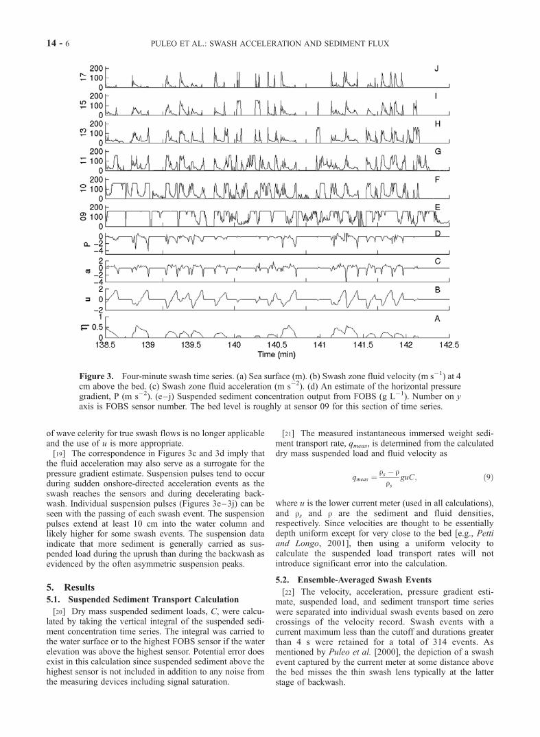
[23] Individual swash events were linearly interpolated toa normalized (by the duration of each swash event) timegrid, tnorm = 0 to 1, such that ensemble averages of themeasurements could be determined (Figure 4). In Figure 4athe ensemble averaged velocity time series is roughlysymmetric with maximum speeds of 0.91 m s�1 duringuprush and 0.89 m s�1 during backwash. The shaded linesrepresent the 5th and 95th percentiles of the individualevents that were used for the ensemble average. Thecorresponding ensemble-averaged accelerations (eventhough the derivative process may amplify noise, we usehai = @u

@t

� �rather than hai = @ uh i

@t ; Figure 4b) show a handlebarshape similar to Figure 1, with a short-lived onshore-directedacceleration during uprush and deceleration during back-wash. The acceleration magnitude (0.5 m s�2) is about halfthat of downslope gravity (0.82 m s�2) for the rest of theensemble average duration. Horizontal pressure gradientestimates are roughly symmetric and largest during timesof strong onshore-directed acceleration and smallest whenacceleration is offshore-directed (Figure 4c). The largespread in P during the beginning and end of the cycle likelyresults from the estimation method since the velocity (used inTaylor’s hypothesis to convert a spatial gradient to a temporalgradient) can be either positive or negative. Unlike thevelocity magnitude, acceleration, and pressure gradient timeseries, ensemble-averaged suspended loads are asymmetric

and indicate that uprush suspended loads are typically twicethat of backwash suspended loads (Figure 4c). Solid circles(squares) in Figure 4 indicate the timing of the uprush(backwash) suspended load maximum. During uprush, thesuspended load maximum tends to lag the accelerationmagnitude maximum by 0.06 (normalized time, i.e., for a10-s swash event, by 0.6 s or 22�) and slightly lead thevelocity magnitude maximum (0.04 normalized time). Con-versely, during backwash, the suspended load maximumleads the onshore-directed backwash acceleration maximumby 0.08 (normalized time) but does not lag or lead thebackwash velocity maximum.

5.3. Suspended Sediment Observations

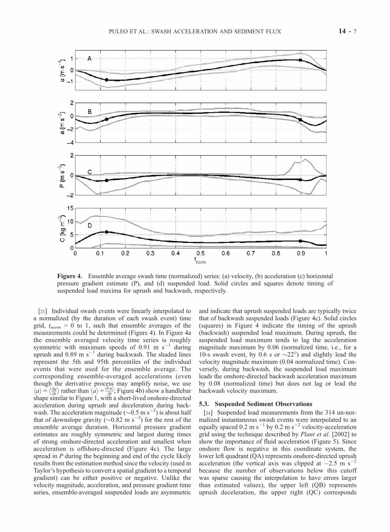
[24] Suspended load measurements from the 314 un-nor-malized instantaneous swash events were interpolated to anequally spaced 0.2 m s�1 by 0.2 m s�2 velocity-accelerationgrid using the technique described by Plant et al. [2002] toshow the importance of fluid acceleration (Figure 5). Sinceonshore flow is negative in this coordinate system, thelower left quadrant (QA) represents onshore-directed uprushacceleration (the vertical axis was clipped at �2.5 m s�2

because the number of observations below this cutoffwas sparse causing the interpolation to have errors largerthan estimated values), the upper left (QB) representsuprush deceleration, the upper right (QC) corresponds

Figure 4. Ensemble average swash time (normalized) series: (a) velocity, (b) acceleration (c) horizontalpressure gradient estimate (P), and (d) suspended load. Solid circles and squares denote timing ofsuspended load maxima for uprush and backwash, respectively.


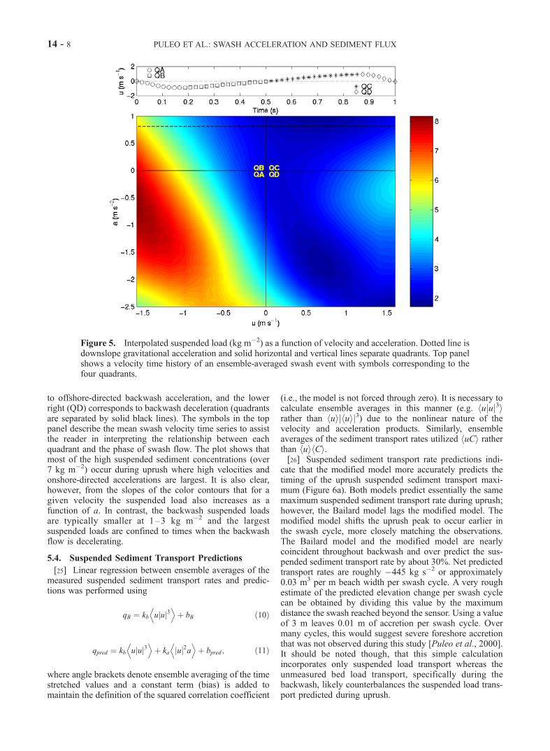
to offshore-directed backwash acceleration, and the lowerright (QD) corresponds to backwash deceleration (quadrantsare separated by solid black lines). The symbols in the toppanel describe the mean swash velocity time series to assistthe reader in interpreting the relationship between eachquadrant and the phase of swash flow. The plot shows thatmost of the high suspended sediment concentrations (over7 kg m�2) occur during uprush where high velocities andonshore-directed accelerations are largest. It is also clear,however, from the slopes of the color contours that for agiven velocity the suspended load also increases as afunction of a. In contrast, the backwash suspended loadsare typically smaller at 1–3 kg m�2 and the largestsuspended loads are confined to times when the backwashflow is decelerating.

5.4. Suspended Sediment Transport Predictions

[25] Linear regression between ensemble averages of themeasured suspended sediment transport rates and predic-tions was performed using

qB ¼ kb u uj j3D E

þ bB ð10Þ

qpred ¼ kb u uj j3D E

þ ka uj j2aD E

þ bpred ; ð11Þ

where angle brackets denote ensemble averaging of the timestretched values and a constant term (bias) is added tomaintain the definition of the squared correlation coefficient

(i.e., the model is not forced through zero). It is necessary tocalculate ensemble averages in this manner (e.g. hujuj3irather than huijhuij3) due to the nonlinear nature of thevelocity and acceleration products. Similarly, ensembleaverages of the sediment transport rates utilized huCi ratherthan huihCi.[26] Suspended sediment transport rate predictions indi-

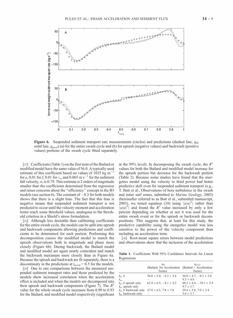
cate that the modified model more accurately predicts thetiming of the uprush suspended sediment transport maxi-mum (Figure 6a). Both models predict essentially the samemaximum suspended sediment transport rate during uprush;however, the Bailard model lags the modified model. Themodified model shifts the uprush peak to occur earlier inthe swash cycle, more closely matching the observations.The Bailard model and the modified model are nearlycoincident throughout backwash and over predict the sus-pended sediment transport rate by about 30%. Net predictedtransport rates are roughly �445 kg s�2 or approximately0.03 m3 per m beach width per swash cycle. A very roughestimate of the predicted elevation change per swash cyclecan be obtained by dividing this value by the maximumdistance the swash reached beyond the sensor. Using a valueof 3 m leaves 0.01 m of accretion per swash cycle. Overmany cycles, this would suggest severe foreshore accretionthat was not observed during this study [Puleo et al., 2000].It should be noted though, that this simple calculationincorporates only suspended load transport whereas theunmeasured bed load transport, specifically during thebackwash, likely counterbalances the suspended load trans-port predicted during uprush.

Figure 5. Interpolated suspended load (kg m�2) as a function of velocity and acceleration. Dotted line isdownslope gravitational acceleration and solid horizontal and vertical lines separate quadrants. Top panelshows a velocity time history of an ensemble-averaged swash event with symbols corresponding to thefour quadrants.


[27] Coefficients (Table 1) on the first term of the Bailard ormodifiedmodel have the same value of 56.0. A typically usedestimate of this coefficient based on values of 1025 kg m�3

for r, 0.01 for f, 0.01 for es, and 0.065 m s�1 for the sedimentfall velocity,w, is 0.79. This estimate is 2 orders of magnitudesmaller than the coefficients determined from the regressionand raises concerns about the ‘‘efficiency’’ concept in the B3models (see section 6). The constant of�8.3 for both modelsshows that there is a slight bias. The fact that this bias isnegative means that suspended sediment transport is notpredicted to occur until the velocity moment and accelerationterms reach some threshold values, analogous to the thresh-old criterion in a Shield’s stress formulation.[28] Although less desirable than calibrating coefficients

for the entire swash cycle, the models can be split into uprushand backwash components allowing predictions and coeffi-cients to be determined for each portion. Performing thisdecomposition causes the modified model to match theuprush observations both in magnitude and phase moreclosely (Figure 6b). During backwash, the Bailard modeland modified model are again nearly coincident and matchthe backwash maximum more closely than in Figure 6a.Because the uprush and backwash are fit separately, there is adiscontinuity in the predictions at tnorm = 0.5 for the models.[29] One to one comparisons between the measured sus-

pended sediment transport rates and those predicted by themodels show increased correlation when the accelerationeffect is included and when the models are decomposed intotheir uprush and backwash components (Figure 7). The R2

value for the whole swash cycle increases from 0.90 to 0.93for the Bailard, and modified model respectively (significant

at the 99% level). In decomposing the swash cycle, the R2

values for both the Bailard and modified model increase forthe uprush portion but decrease for the backwash portion(Table 2). Because some studies have found that the ener-getics model using the velocity to third power had betterpredictive skill even for suspended sediment transport (e.g.,T. Butt et al., Observations of bore turbulence in the swashand inner surf zones, submitted to Marine Geology, 2003)(hereinafter referred to as Butt et al., submitted manuscript,2003), we tested equation (10) using hujuj2i rather thanhujuj3i and found the R2 value increased by only a fewpercent depending on whether or not it was used for theentire swash event or for the uprush or backwash decom-positions. This suggests that, at least for this study, thepredictive capability using the energetics model was lesssensitive to the power of the velocity component thanincluding an acceleration term.[30] Root-mean square errors between model predictions

and observations show that the inclusion of the acceleration

Table 1. Coefficients With 95% Confidence Intervals for Linear

Regressions

qB(Bailard, No Acceleration

Terms)

qpred(Bailard + Acceleration

Terms)

kb, b 56.0 ± 5.4, �8.3 ± 3.4 56.0 ± 4.7, �8.3 ± 3.0ka, – 9.3 ± 4.9kb, b uprush only 62.4 ± 6.5, �9.1 ± 4.2 60.2 ± 4.4, �10.1 ± 2.9ka, uprush only – 9.7 ± 3.7kb, b backwash only 27.8 ± 6.5, 7.8 ± 3.8 29.4 ± 5.8, 7.0 ± 3.4ka, backwash only – 5.0 ± 3.7

Figure 6. Suspended sediment transport rate measurements (circles) and predictions (dashed line, qB;solid line, qpred) (a) for the entire swash cycle and (b) for uprush (negative values) and backwash (positivevalues) portions of the swash cycle fitted separately.


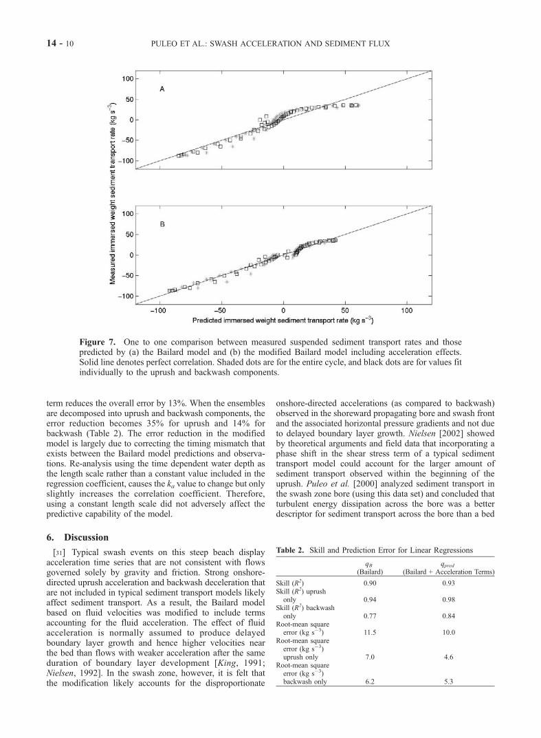
term reduces the overall error by 13%. When the ensemblesare decomposed into uprush and backwash components, theerror reduction becomes 35% for uprush and 14% forbackwash (Table 2). The error reduction in the modifiedmodel is largely due to correcting the timing mismatch thatexists between the Bailard model predictions and observa-tions. Re-analysis using the time dependent water depth asthe length scale rather than a constant value included in theregression coefficient, causes the ka value to change but onlyslightly increases the correlation coefficient. Therefore,using a constant length scale did not adversely affect thepredictive capability of the model.

6. Discussion

[31] Typical swash events on this steep beach displayacceleration time series that are not consistent with flowsgoverned solely by gravity and friction. Strong onshore-directed uprush acceleration and backwash deceleration thatare not included in typical sediment transport models likelyaffect sediment transport. As a result, the Bailard modelbased on fluid velocities was modified to include termsaccounting for the fluid acceleration. The effect of fluidacceleration is normally assumed to produce delayedboundary layer growth and hence higher velocities nearthe bed than flows with weaker acceleration after the sameduration of boundary layer development [King, 1991;Nielsen, 1992]. In the swash zone, however, it is felt thatthe modification likely accounts for the disproportionate

onshore-directed accelerations (as compared to backwash)observed in the shoreward propagating bore and swash frontand the associated horizontal pressure gradients and not dueto delayed boundary layer growth. Nielsen [2002] showedby theoretical arguments and field data that incorporating aphase shift in the shear stress term of a typical sedimenttransport model could account for the larger amount ofsediment transport observed within the beginning of theuprush. Puleo et al. [2000] analyzed sediment transport inthe swash zone bore (using this data set) and concluded thatturbulent energy dissipation across the bore was a betterdescriptor for sediment transport across the bore than a bed

Table 2. Skill and Prediction Error for Linear Regressions

qB(Bailard)

qpred(Bailard + Acceleration Terms)

Skill (R2) 0.90 0.93Skill (R2) uprushonly 0.94 0.98

Skill (R2) backwashonly 0.77 0.84

Root-mean squareerror (kg s�3) 11.5 10.0

Root-mean squareerror (kg s�3)uprush only 7.0 4.6

Root-mean squareerror (kg s�3)backwash only 6.2 5.3

Figure 7. One to one comparison between measured suspended sediment transport rates and thosepredicted by (a) the Bailard model and (b) the modified Bailard model including acceleration effects.Solid line denotes perfect correlation. Shaded dots are for the entire cycle, and black dots are for values fitindividually to the uprush and backwash components.


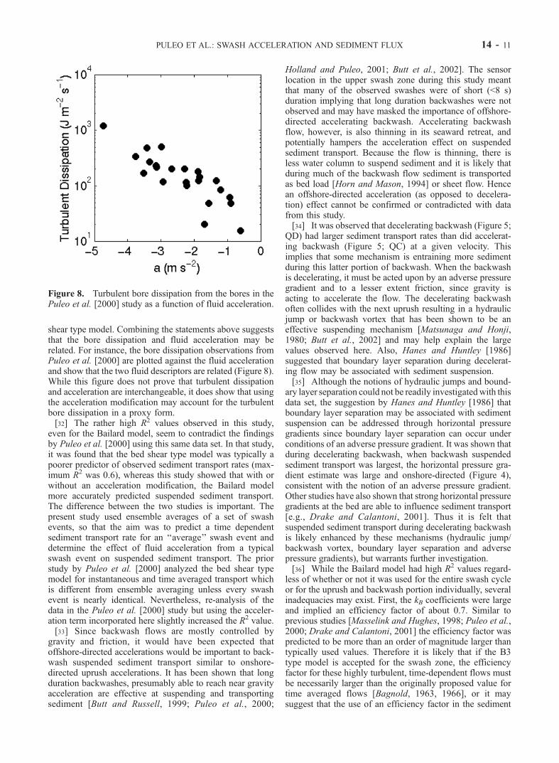
shear type model. Combining the statements above suggeststhat the bore dissipation and fluid acceleration may berelated. For instance, the bore dissipation observations fromPuleo et al. [2000] are plotted against the fluid accelerationand show that the two fluid descriptors are related (Figure 8).While this figure does not prove that turbulent dissipationand acceleration are interchangeable, it does show that usingthe acceleration modification may account for the turbulentbore dissipation in a proxy form.[32] The rather high R2 values observed in this study,

even for the Bailard model, seem to contradict the findingsby Puleo et al. [2000] using this same data set. In that study,it was found that the bed shear type model was typically apoorer predictor of observed sediment transport rates (max-imum R2 was 0.6), whereas this study showed that with orwithout an acceleration modification, the Bailard modelmore accurately predicted suspended sediment transport.The difference between the two studies is important. Thepresent study used ensemble averages of a set of swashevents, so that the aim was to predict a time dependentsediment transport rate for an ‘‘average’’ swash event anddetermine the effect of fluid acceleration from a typicalswash event on suspended sediment transport. The priorstudy by Puleo et al. [2000] analyzed the bed shear typemodel for instantaneous and time averaged transport whichis different from ensemble averaging unless every swashevent is nearly identical. Nevertheless, re-analysis of thedata in the Puleo et al. [2000] study but using the acceler-ation term incorporated here slightly increased the R2 value.[33] Since backwash flows are mostly controlled by

gravity and friction, it would have been expected thatoffshore-directed accelerations would be important to back-wash suspended sediment transport similar to onshore-directed uprush accelerations. It has been shown that longduration backwashes, presumably able to reach near gravityacceleration are effective at suspending and transportingsediment [Butt and Russell, 1999; Puleo et al., 2000;

Holland and Puleo, 2001; Butt et al., 2002]. The sensorlocation in the upper swash zone during this study meantthat many of the observed swashes were of short (<8 s)duration implying that long duration backwashes were notobserved and may have masked the importance of offshore-directed accelerating backwash. Accelerating backwashflow, however, is also thinning in its seaward retreat, andpotentially hampers the acceleration effect on suspendedsediment transport. Because the flow is thinning, there isless water column to suspend sediment and it is likely thatduring much of the backwash flow sediment is transportedas bed load [Horn and Mason, 1994] or sheet flow. Hencean offshore-directed acceleration (as opposed to decelera-tion) effect cannot be confirmed or contradicted with datafrom this study.[34] It was observed that decelerating backwash (Figure 5;

QD) had larger sediment transport rates than did accelerat-ing backwash (Figure 5; QC) at a given velocity. Thisimplies that some mechanism is entraining more sedimentduring this latter portion of backwash. When the backwashis decelerating, it must be acted upon by an adverse pressuregradient and to a lesser extent friction, since gravity isacting to accelerate the flow. The decelerating backwashoften collides with the next uprush resulting in a hydraulicjump or backwash vortex that has been shown to be aneffective suspending mechanism [Matsunaga and Honji,1980; Butt et al., 2002] and may help explain the largevalues observed here. Also, Hanes and Huntley [1986]suggested that boundary layer separation during decelerat-ing flow may be associated with sediment suspension.[35] Although the notions of hydraulic jumps and bound-

ary layer separation could not be readily investigatedwith thisdata set, the suggestion by Hanes and Huntley [1986] thatboundary layer separation may be associated with sedimentsuspension can be addressed through horizontal pressuregradients since boundary layer separation can occur underconditions of an adverse pressure gradient. It was shown thatduring decelerating backwash, when backwash suspendedsediment transport was largest, the horizontal pressure gra-dient estimate was large and onshore-directed (Figure 4),consistent with the notion of an adverse pressure gradient.Other studies have also shown that strong horizontal pressuregradients at the bed are able to influence sediment transport[e.g., Drake and Calantoni, 2001]. Thus it is felt thatsuspended sediment transport during decelerating backwashis likely enhanced by these mechanisms (hydraulic jump/backwash vortex, boundary layer separation and adversepressure gradients), but warrants further investigation.[36] While the Bailard model had high R2 values regard-

less of whether or not it was used for the entire swash cycleor for the uprush and backwash portion individually, severalinadequacies may exist. First, the kB coefficients were largeand implied an efficiency factor of about 0.7. Similar toprevious studies [Masselink and Hughes, 1998; Puleo et al.,2000; Drake and Calantoni, 2001] the efficiency factor waspredicted to be more than an order of magnitude larger thantypically used values. Therefore it is likely that if the B3type model is accepted for the swash zone, the efficiencyfactor for these highly turbulent, time-dependent flows mustbe necessarily larger than the originally proposed value fortime averaged flows [Bagnold, 1963, 1966], or it maysuggest that the use of an efficiency factor in the sediment

Figure 8. Turbulent bore dissipation from the bores in thePuleo et al. [2000] study as a function of fluid acceleration.


transport formulation is undesirable. Second, the B3 typemodel, assumes that instantaneous sediment transport ratesare a function of instantaneous flow conditions. Because ofthis assumption, pre-suspended sediment advection (fromthe inner surf zone or the bore) is not accounted for.Unfortunately, in the swash zone, where hydraulic jumpsand bore collapse appear to be dominant sediment suspend-ing mechanisms, the exclusion of advected sediment andwater column storage of sediment [Kobayashi and Johnson,2001] should be expected to cause errors in the B3 ap-proach. Studies by Puleo et al. [2000] and Butt et al.(submitted manuscript, 2003), however, showed that sedi-ment tends to settle out quickly behind the shorewardpropagating bore such that the lack of pre-suspendedsediment advection in the B3 type swash zone sedimenttransport model may not represent a significant source oferror.

7. Conclusion

[37] Suspended sediment concentrations and fluid veloc-ities collected in the swash zone of a high energy, steepbeach showed that high values of suspended sedimentconcentration (over 7 kg m�2) were observed during timesof rapid velocities, uprush acceleration and onshore directedpressure gradients during uprush associated with the shore-ward propagating bore. Maximum suspended sedimentconcentrations reached 3 kg m�2 during backwash butoccurred during decelerating flow, when the backwash islikely slowed by adverse pressure gradients from the ensu-ing uprush. An energetics model for sediment transport wasmodified to include the effect of fluid acceleration and wasable to reduce the root-mean square prediction error by upto 35% over the energetics model without the modificationsuggesting that the inclusion of the acceleration term mayaccount for the additional sediment transporting mecha-nisms during the unsteady flow conditions observed in theswash zone.

[38] Acknowledgments. J. A. P., K. T. H. and N. G. P. weresupported by the Office of Naval Research (ONR) through base fundingto the Naval Research Laboratory (PE#61153N). DNS was supported byONR (grant N00014-01-1-0152). We thank Rob Holman and Reggie Beachfor allowing us to utilize the Gleneden data set and Joe Calantoni for hiscomments.

ReferencesAdmiraal, D. M., M. H. Garcia, and J. F. Rodriguez, Entrainment responseof bed sediment to time-varying flows, Water Resour. Res., 36(1), 335–348, 2000.

Bagnold, R. A., Mechanics of marine sedimentation, in The Sea, edited byM. N. Hill, pp. 507–528, Wiley-Intersci., Hoboken, N. J., 1963.

Bagnold, R. A., An approach to the sediment transport problem from gen-eral physics, report, 37 pp., U.S. Geol. Surv., Washington, D. C., 1966.

Bailard, J. A., An energetics total load sediment transport model for a planesloping beach, J. Geophys. Res., 86(C11), 938–954, 1981.

Beach, R. A., and R. W. Sternberg, Infragravity driven suspended sedimenttransport in the swash, inner and outer-surf zone, in Coastal Sediments’91, edited by N. C. Kraus, K. J. Gingerich, and D. L. Kriebel, pp. 114–128, Am. Soc. of Civ. Eng., Seattle, Wash., 1991.

Bowen, A. J., Simple models of nearshore sedimentation: Beach profilesand longshore bars, in The Coastline of Canada, edited by S. B. McCann,pp. 1–11, Geol. Surv. of Can., Ottawa, Ont., Can., 1980.

Butt, T., and P. Russell, Suspended sediment transport mechanisms in high-energy swash, Mar. Geol., 161(2–4), 361–375, 1999.

Butt, T., P. Russell, and I. Turner, The influence of swash infiltration-exfiltration on beach face sediment transport: Onshore or offshore?,Coastal Eng., 42(1), 35–52, 2001.

Butt, T., P. Russell, G. Masselink, J. Miles, D. Huntley, D. Evans, andP. Ganderton, An integrative approach to investigating the role of swashin shoreline change, paper presented at 28th International Conference onCoastal Engineering, Am. Soc. of Civ. Eng., Cardiff, Wales, 2002.

Butt, T., P. Russell, J. A. Puleo, J. Miles, and G. Masselink, Observations ofbore turbulence in the swash and inner surf zones, Marine Geology,submitted.

Cowen, E. A., I. M. Sou, P. L.-F. Liu, and B. Raubenheimer, PIV measure-ments within a laboratory generated swash zone, J. Eng. Mech., 129,1119, 2003.

Drake, T. G., and J. Calantoni, Discrete particle model for sheet flowsediment transport in the nearshore, J. Geophys. Res., 106(C9),19,859–19,868, 2001.

Elgar, S., E. L. Gallagher, and R. T. Guza, Nearshore sandbar migration,J. Geophys. Res., 106(C6), 11,623–11,627, 2001.

Gallagher, E. L., S. Elgar, and R. T. Guza, Observations of sand bar evolu-tion on a natural beach, J. Geophys. Res., 103(C2), 3203–3215, 1998.

Hanes, D. M., and D. A. Huntley, Continuous measurements of suspendedsand concentration in a wave dominated nearshore environment, Cont.Shelf Res., 6(4), 585–596, 1986.

Hardisty, J., J. Collier, and D. Hamilton, A calibration of the Bagnold beachequation, Mar. Geol., 61(1), 95–101, 1984.

Ho, D. V., and R. E. Meyer, Climb of a bore on a beach: 1. Uniform beachslope, J. Fluid Mech., 14(20), 305–318, 1962.

Hoefel, F., and S. Elgar, Surfzone sandbar migration and wave accelerationinduced sediment transport, Science, 299, 1885, 2003.

Holland, K. T., and J. A. Puleo, Variable swash motions associated withforeshore profile change, J. Geophys. Res., 106(C3), 4613–4623, 2001.

Horn, D. P., and T. Mason, Swash zone sediment transport modes, Mar.Geol., 120(3–4), 309–325, 1994.

Hughes, M. G., G. Masselink, and R. W. Brander, Flow velocity and sedi-ment transport in the swash zone of a steep beach, Mar. Geol., 138(1–2),91–103, 1997.

Jaffe, B. E., and D. M. Rubin, Using nonlinear forecasting to learn themagnitude and phasing of time-varying sediment suspension in the surfzone, J. Geophys. Res., 101(C6), 14,283–14,296, 1996.

Johnson, R. S., A Modern Introduction to the Mathematical Theory ofWater Waves, 445 pp., Cambridge Univ. Press, New York, 1997.

King, D. B. J., Studies in oscillatory flow bedload sediment transport, Ph.D.thesis, Univ. of Calif., San Diego, San Diego, Calif., 1991.

Kirkgoz, M. S., A theoretical study of plunging breakers and their run-up,Coastal Eng., 5(4), 353–370, 1981.

Kobayashi, N., and B. D. Johnson, Sand suspension, storage, advection,and settling in surf and swash zones, J. Geophys. Res., 106(C5), 9363–9376, 2001.

Masselink, G., and M. Hughes, Field investigation of sediment transport inthe swash zone, Cont. Shelf Res., 18(10), 1179–1199, 1998.

Matsunaga, N., and H. Honji, The backwash vortex, J. Fluid Mech.,99(AUG), 813–815, 1980.

Meyer-Peter, E., and R. Muller, Formulas for bed-load transport, paper pre-sented at 3rd Meeting, Int. Assoc. for Hydraul. Res., Delft, Netherlands,1948.

Nielsen, P., Coastal Bottom Boundary Layers and Sediment Transport,324 pp., World Sci., River Edge, N. J., 1992.

Nielsen, P., Shear stress and sediment transport calculations for swash zonemodelling, Coastal Eng., 45(1), 53–60, 2002.

Osborne, P. D., and G. A. Rooker, Sand re-suspension events in a highenergy infragravity swash zone, J. Coastal Res., 15(1), 74–86, 1999.

Petti, M., and S. Longo, Turbulence experiments in the swash zone, CoastalEng., 43(1), 1–24, 2001.

Plant, N., K. T. Holland, and J. A. Puleo, Analysis of the scale of errors innearshore bathymetric interpolation, Mar. Geol., 191, 71–86, 2002.

Puleo, J. A., and K. T. Holland, Estimating swash zone friction coefficientson a sandy beach, Coastal Eng., 43(1), 25–40, 2001.

Puleo, J. A., R. A. Beach, R. A. Holman, and J. S. Allen, Swash zonesediment suspension and transport and the importance of bore-generatedturbulence, J. Geophys. Res., 105(C7), 17,021–17,044, 2000.

Shen, M. C., and R. E. Meyer, Climb of a bore on a beach: 3. Run-up,J. Fluid Mech., 16(8), 113–125, 1963.

Thornton, E. B., R. T. Humiston, and W. Birkemeier, Bar/trough generationon a natural beach, J. Geophys. Res., 101(C5), 12,097–12,110, 1996.

��D. M. Hanes, and D. N. Slinn, University of Florida, Civil and Coastal

Engineering Department, Gainesville, FL 32611-6590, USA. ([email protected]; [email protected])K. T. Holland, N. G. Plant, and J. A. Puleo, Naval Research Laboratory,

Code 74403, Stennis Space Center, MS 39529, USA. ([email protected]; [email protected]; [email protected])


Documents

Fluid acceleration effects on suspended sediment transport in the