FLUENT IC Tut 02 Layering Approach

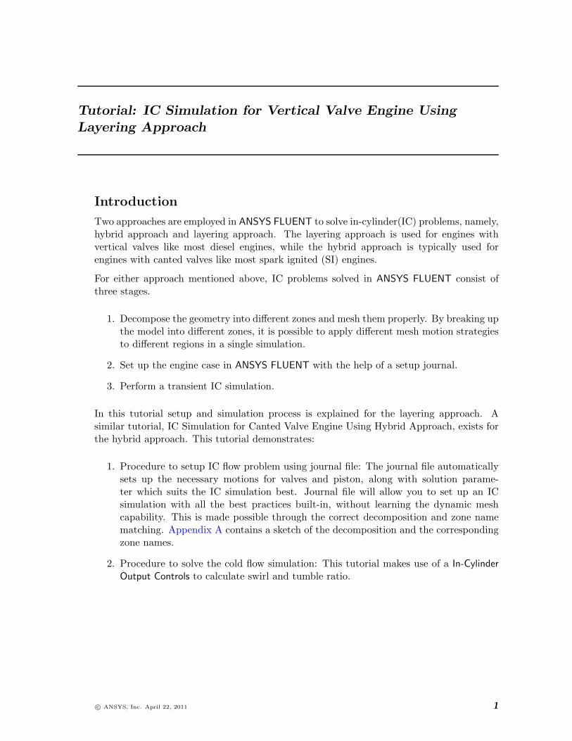
Tutorial: IC Simulation for Vertical Valve Engine Using

Layering Approach

Introduction

Two approaches are employed in ANSYS FLUENT to solve in-cylinder(IC) problems, namely,hybrid approach and layering approach. The layering approach is used for engines withvertical valves like most diesel engines, while the hybrid approach is typically used forengines with canted valves like most spark ignited (SI) engines.

For either approach mentioned above, IC problems solved in ANSYS FLUENT consist ofthree stages.

1. Decompose the geometry into different zones and mesh them properly. By breaking upthe model into different zones, it is possible to apply different mesh motion strategiesto different regions in a single simulation.

2. Set up the engine case in ANSYS FLUENT with the help of a setup journal.

3. Perform a transient IC simulation.

In this tutorial setup and simulation process is explained for the layering approach. Asimilar tutorial, IC Simulation for Canted Valve Engine Using Hybrid Approach, exists forthe hybrid approach. This tutorial demonstrates:

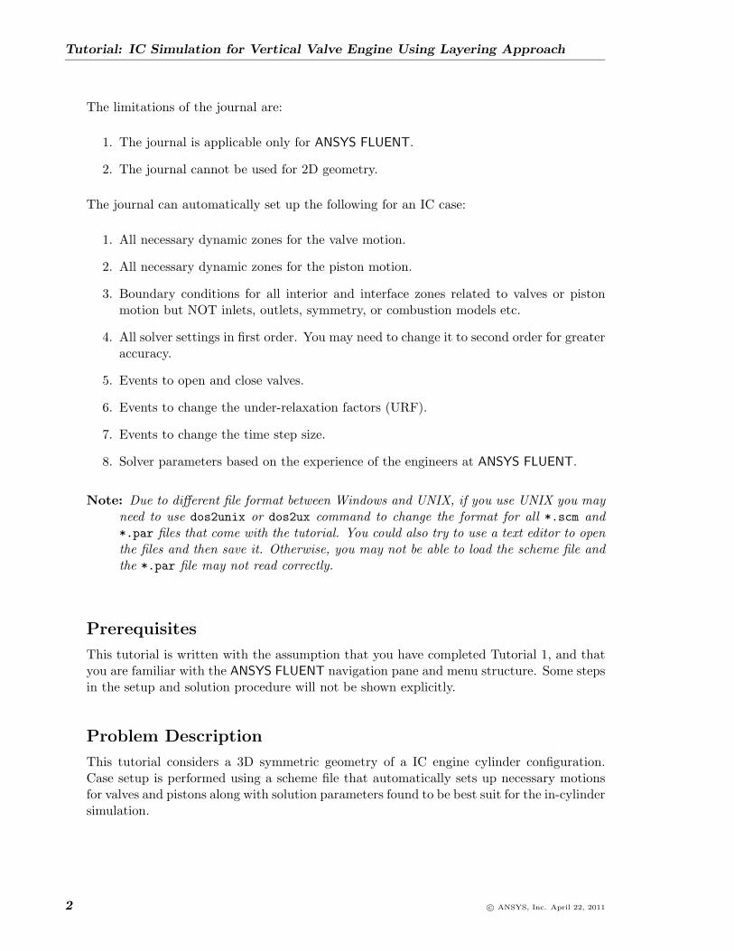
1. Procedure to setup IC flow problem using journal file: The journal file automaticallysets up the necessary motions for valves and piston, along with solution parame-ter which suits the IC simulation best. Journal file will allow you to set up an ICsimulation with all the best practices built-in, without learning the dynamic meshcapability. This is made possible through the correct decomposition and zone namematching. Appendix A contains a sketch of the decomposition and the correspondingzone names.

2. Procedure to solve the cold flow simulation: This tutorial makes use of a In-CylinderOutput Controls to calculate swirl and tumble ratio.

c© ANSYS, Inc. April 22, 2011 1

Tutorial: IC Simulation for Vertical Valve Engine Using Layering Approach

The limitations of the journal are:

1. The journal is applicable only for ANSYS FLUENT.

2. The journal cannot be used for 2D geometry.

The journal can automatically set up the following for an IC case:

1. All necessary dynamic zones for the valve motion.

2. All necessary dynamic zones for the piston motion.

3. Boundary conditions for all interior and interface zones related to valves or pistonmotion but NOT inlets, outlets, symmetry, or combustion models etc.

4. All solver settings in first order. You may need to change it to second order for greateraccuracy.

5. Events to open and close valves.

6. Events to change the under-relaxation factors (URF).

7. Events to change the time step size.

8. Solver parameters based on the experience of the engineers at ANSYS FLUENT.

Note: Due to different file format between Windows and UNIX, if you use UNIX you mayneed to use dos2unix or dos2ux command to change the format for all *.scm and*.par files that come with the tutorial. You could also try to use a text editor to openthe files and then save it. Otherwise, you may not be able to load the scheme file andthe *.par file may not read correctly.

Prerequisites

This tutorial is written with the assumption that you have completed Tutorial 1, and thatyou are familiar with the ANSYS FLUENT navigation pane and menu structure. Some stepsin the setup and solution procedure will not be shown explicitly.

Problem Description

This tutorial considers a 3D symmetric geometry of a IC engine cylinder configuration.Case setup is performed using a scheme file that automatically sets up necessary motionsfor valves and pistons along with solution parameters found to be best suit for the in-cylindersimulation.

2 c© ANSYS, Inc. April 22, 2011


Figure 1: Geometry Decomposition

Setup and Solution

Preparation

1. Copy the files, (IC tutorial IIb.msh.gz, R 13 IC scheme.scm,IC-motion-parameters.par, and valve.prof) to your working folder.

2. Use FLUENT Launcher to start the 3D version of ANSYS FLUENT.

For more information about FLUENT Launcher refer to Section 1.1.2 in the ANSYSFLUENT 13.0 User’s Guide.

3. Enable Double-Precision in the Display Options list.

4. Click the Environment tab and ensure that Setup Compilation Environment for UDF isenabled.

The path to the .bat file which is required to compile the UDF will be displayed assoon as you enable Setup Compilation Environment for UDF.

If the Environment tab does not appear in the FLUENT Launcher dialog box by default,click the Show More Options button to view the additional settings.

Note: The Display Options are enabled by default. Therefore, after you read in themesh, it will be displayed in the embedded graphics window.



Step 1: Mesh

1. Read the mesh file, IC tutorial IIb.msh.gz.

File −→ Read −→Mesh...

As ANSYS FLUENT reads the mesh file, messages will appear in the console reportingthe progress of the conversion.

Note: Only inlet valve is modeled in the tutorial. The simulation will be done onlyfor the intake stroke.

Step 2: General Settings

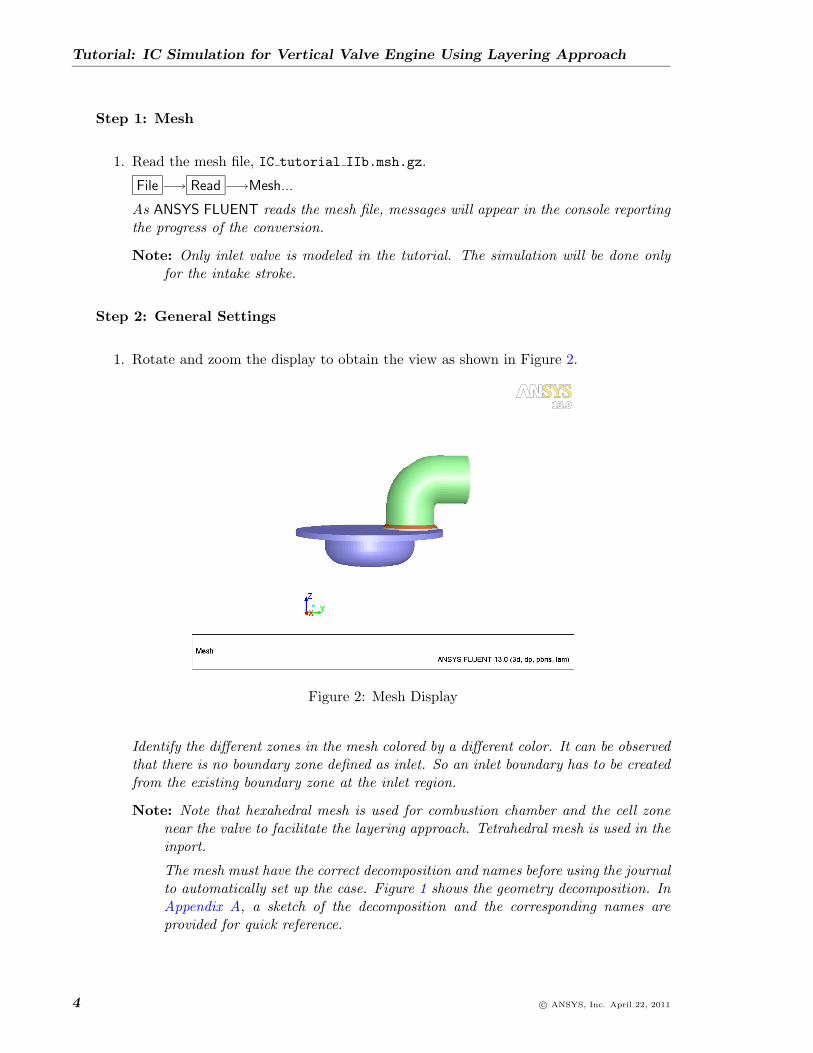
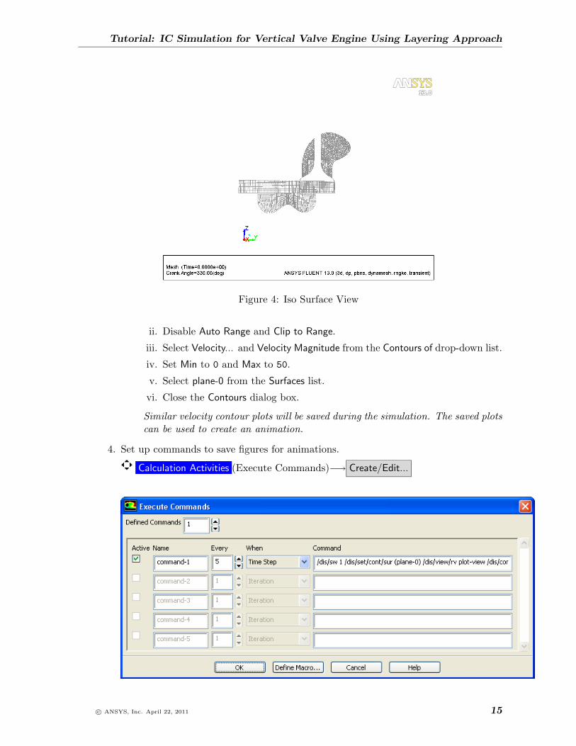
1. Rotate and zoom the display to obtain the view as shown in Figure 2.

Figure 2: Mesh Display

Identify the different zones in the mesh colored by a different color. It can be observedthat there is no boundary zone defined as inlet. So an inlet boundary has to be createdfrom the existing boundary zone at the inlet region.

Note: Note that hexahedral mesh is used for combustion chamber and the cell zonenear the valve to facilitate the layering approach. Tetrahedral mesh is used in theinport.

The mesh must have the correct decomposition and names before using the journalto automatically set up the case. Figure 1 shows the geometry decomposition. InAppendix A, a sketch of the decomposition and the corresponding names areprovided for quick reference.



2. Check the mesh.

General −→ Check

ANSYS FLUENT will perform various checks on the mesh and report the progress inthe console. Ensure that the minimum volume reported is a positive number.

Warnings will be displayed regarding unassigned interface zones, resulting in the failureof the mesh check. You do not need to take any action at this point, as this issue willbe rectified when you define the mesh interfaces in a later step.

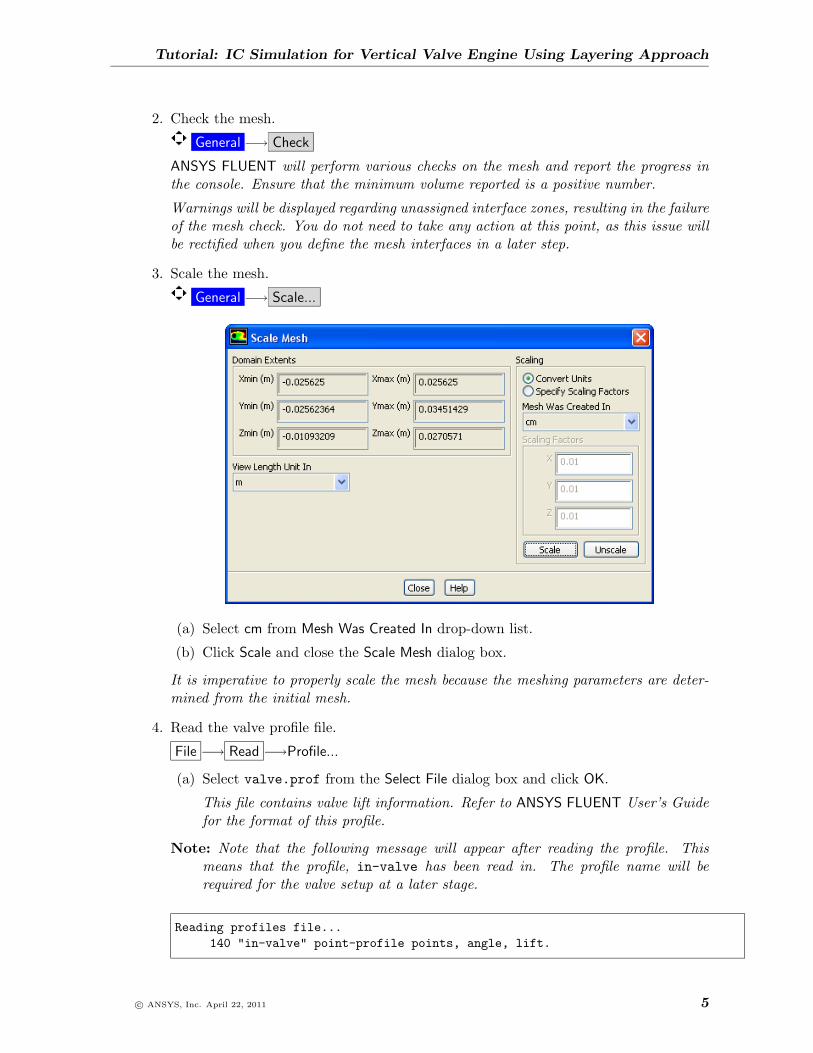
3. Scale the mesh.

General −→ Scale...

(a) Select cm from Mesh Was Created In drop-down list.

(b) Click Scale and close the Scale Mesh dialog box.

It is imperative to properly scale the mesh because the meshing parameters are deter-mined from the initial mesh.

4. Read the valve profile file.

File −→ Read −→Profile...

(a) Select valve.prof from the Select File dialog box and click OK.

This file contains valve lift information. Refer to ANSYS FLUENT User’s Guidefor the format of this profile.

Note: Note that the following message will appear after reading the profile. Thismeans that the profile, in-valve has been read in. The profile name will berequired for the valve setup at a later stage.

Reading profiles file...140 "in-valve" point-profile points, angle, lift.



5. Read the scheme file.

File −→ Read −→Scheme...

(a) Select R 13 IC scheme.scm from the Select File dialog box and click OK.

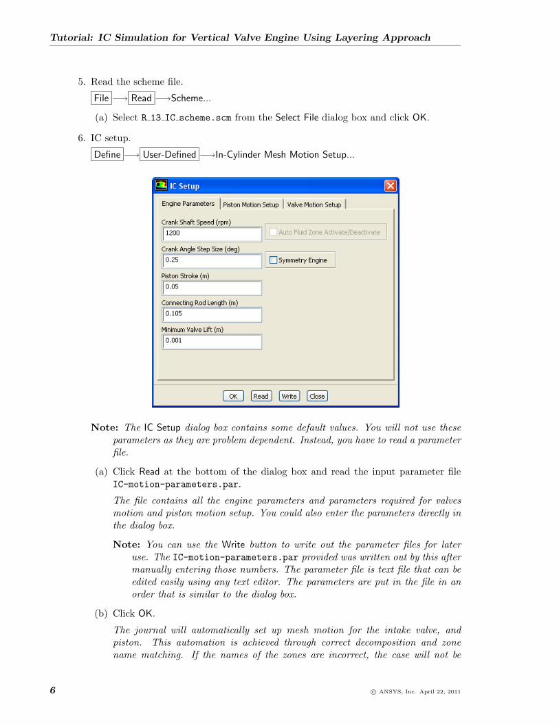
6. IC setup.

Define −→ User-Defined −→In-Cylinder Mesh Motion Setup...

Note: The IC Setup dialog box contains some default values. You will not use theseparameters as they are problem dependent. Instead, you have to read a parameterfile.

(a) Click Read at the bottom of the dialog box and read the input parameter fileIC-motion-parameters.par.

The file contains all the engine parameters and parameters required for valvesmotion and piston motion setup. You could also enter the parameters directly inthe dialog box.

Note: You can use the Write button to write out the parameter files for lateruse. The IC-motion-parameters.par provided was written out by this aftermanually entering those numbers. The parameter file is text file that can beedited easily using any text editor. The parameters are put in the file in anorder that is similar to the dialog box.

(b) Click OK.

The journal will automatically set up mesh motion for the intake valve, andpiston. This automation is achieved through correct decomposition and zonename matching. If the names of the zones are incorrect, the case will not be



setup and the you will be notified about the zones for which the names are notmatched. The scheme file will automatically select Standard k-e as the turbulencemodel.

Note: The explanation of the parameters is in Appendix B. For this tutorial,Conformal Setup is used. More details on different Layering Setup Type areexplained in Appendix C.

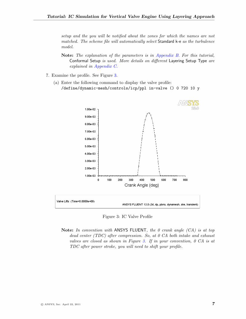
7. Examine the profile. See Figure 3.

(a) Enter the following command to display the valve profile:/define/dynamic-mesh/controls/icp/ppl in-valve () 0 720 10 y

Figure 3: IC Valve Profile

Note: In convention with ANSYS FLUENT, the 0 crank angle (CA) is at topdead center (TDC) after compression. So, at 0 CA both intake and exhaustvalves are closed as shown in Figure 3. If in your convention, 0 CA is atTDC after power stroke, you will need to shift your profile.



Step 3: Models

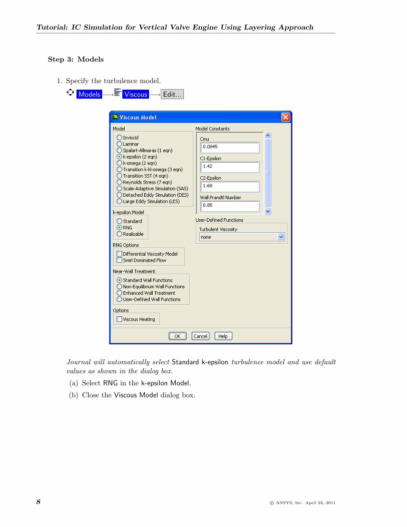
1. Specify the turbulence model.

Models −→ Viscous −→ Edit...

Journal will automatically select Standard k-epsilon turbulence model and use defaultvalues as shown in the dialog box.

(a) Select RNG in the k-epsilon Model.

(b) Close the Viscous Model dialog box.



Step 4: Zone Motion Preview

1. Set up mesh display.

General −→ Display

(a) Enable Edges and disable Faces from the Options group box.

(b) Select Outline from the Edge Type group box.

(c) Click Display and close the Mesh Display dialog box.

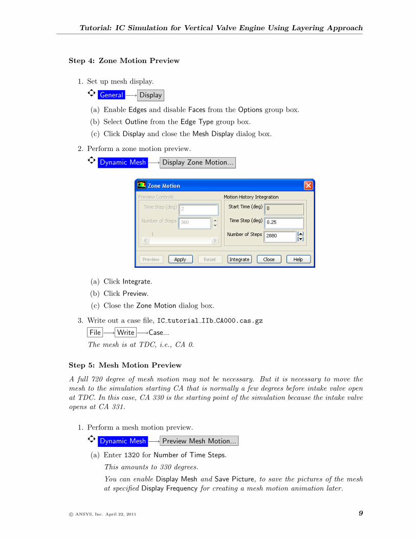
2. Perform a zone motion preview.

Dynamic Mesh −→ Display Zone Motion...

(a) Click Integrate.

(b) Click Preview.

(c) Close the Zone Motion dialog box.

3. Write out a case file, IC tutorial IIb CA000.cas.gz

File −→ Write −→Case...

The mesh is at TDC, i.e., CA 0.

Step 5: Mesh Motion Preview

A full 720 degree of mesh motion may not be necessary. But it is necessary to move themesh to the simulation starting CA that is normally a few degrees before intake valve openat TDC. In this case, CA 330 is the starting point of the simulation because the intake valveopens at CA 331.

1. Perform a mesh motion preview.

Dynamic Mesh −→ Preview Mesh Motion...

(a) Enter 1320 for Number of Time Steps.

This amounts to 330 degrees.

You can enable Display Mesh and Save Picture, to save the pictures of the meshat specified Display Frequency for creating a mesh motion animation later.



(b) Click Apply.

(c) Click Preview.

(d) Close the Mesh Motion dialog box after the preview is completed.

Note: Mesh motion for this tutorial case takes about one hour on serial WindowsXP 3.19GHz machine.

Step 6: Boundary Conditions

Boundary Conditions

1. Specify the inlet boundary conditions.

Boundary Conditions −→ inlet −→ Edit...

(a) Select Intensity and Hydraulic Diameter from the Specification Method drop-downlist in the Turbulence group box.

(b) Enter 2 % for Turbulent Intensity.

(c) Enter 0.0172 m for the Hydraulic Diameter.

(d) Click OK to close the Pressure Inlet dialog box.

There is no need to specify boundary conditions for other face zones. Those will beautomatically setup by the scheme.

2. Write out a case file, IC tutorial IIb CA330.cas.gz.

File −→ Write −→Case...

Step 7: Dynamic Mesh

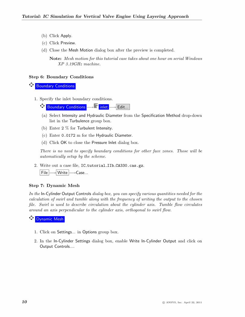
In the In-Cylinder Output Controls dialog box, you can specify various quantities needed for thecalculation of swirl and tumble along with the frequency of writing the output to the chosenfile. Swirl is used to describe circulation about the cylinder axis. Tumble flow circulatesaround an axis perpendicular to the cylinder axis, orthogonal to swirl flow.

Dynamic Mesh

1. Click on Settings... in Options group box.

2. In the In-Cylinder Settings dialog box, enable Write In-Cylinder Output and click onOutput Controls....



(a) In the In-Cylinder Output Controls dialog box, set In-Cylinder Data Write Frequencyto 1.

(b) Ensure center of gravity is selected from Swirl Center Method.

(c) From the Cell Zones list select fluid-bowl, fluid-ch-invalve, fluid-ch-lower, and fluid-ch-upper.

(d) Set X, Y, Z from Swirl Axis to 0, 0, 1 respectively.

(e) Set X, Y, Z from Tumble X-Axis to 0.015, 0.005, 0 respectively.

(f) Set X, Y, Z from Tumble Y-Axis to -0.005, 0.015, 0 respectively.

(g) Enter ic-layer.txt for File Name.

(h) Click OK.

3. Click OK in the In-Cylinder Settings dialog box to close it.



Step 8: Solution

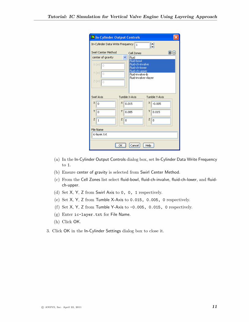
1. Set up solution methods

Solution Methods

(a) Retain the selection of Least Squares Cell Based from Gradient and PRESTO! fromPressure.

(b) Select Second Order Upwind as the Spatial Discretization for all the other variables.

2. Initialize the flow.

Solution Initialization −→ Initialize

3. Create a velocity magnitude contour plot.

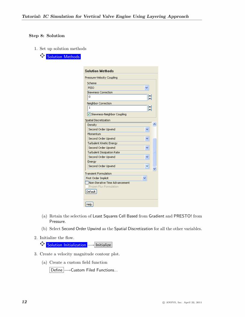
(a) Create a custom field function

Define −→Custom Filed Functions...



i. Select Mesh... and Y-Coordinate from Field Functions drop-down lists.

ii. Click Select.

iii. Click +.

iv. Enter 2.2727 using the buttons in the Custom Field Function Calculator dialogbox.

v. Click X.

vi. Select Mesh... and X-Coordinate from Field Functions drop-down lists.

vii. Click Select.

viii. Enter plane as the New Function Name.

ix. Click Define and close the dialog box.

(b) Create an iso surface.

Surface −→Iso-Surface...

i. Select Custom Field Function... and plane from the list of Surface of Constant.



ii. Retain 0 for Iso-Values.

iii. Enter plane-0 for New Surface Name.

iv. Click Compute and then Create.

v. Close the Iso-Surface dialog box.

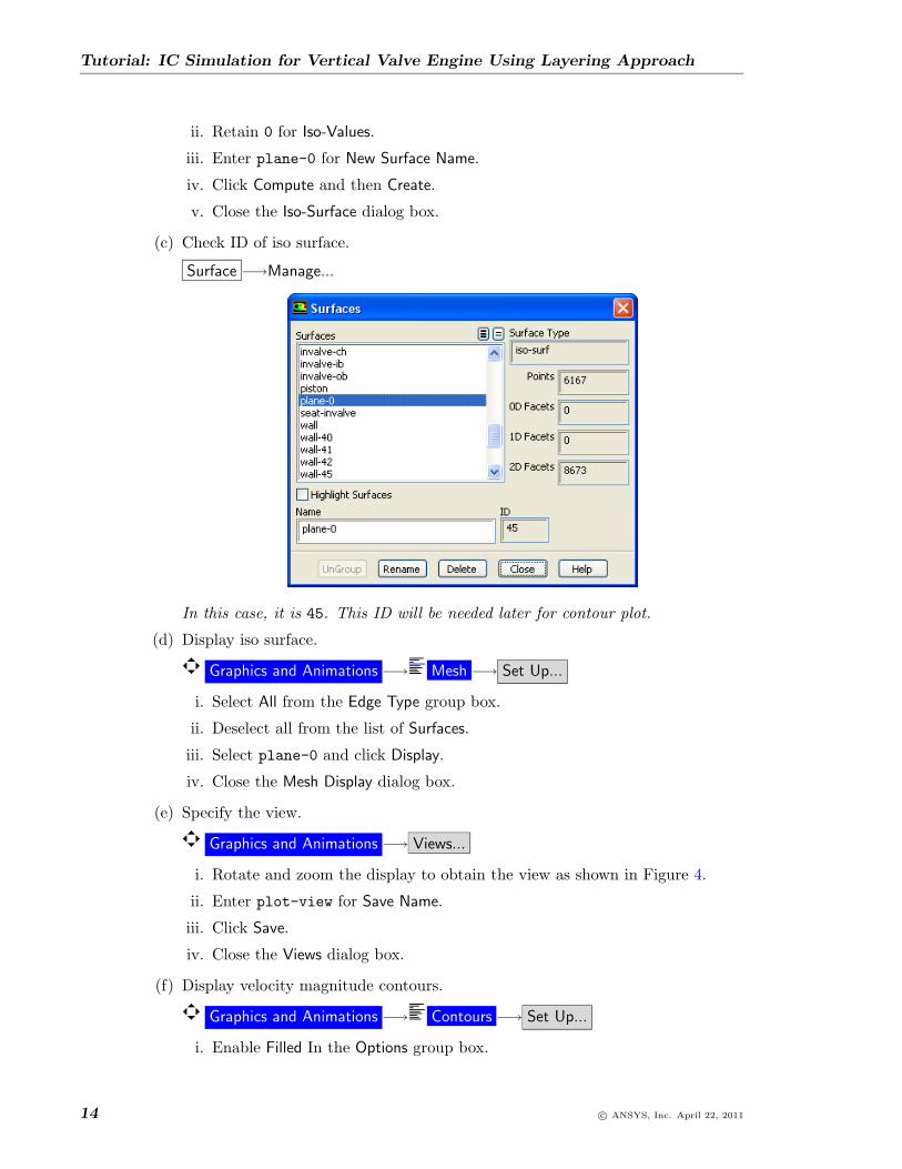
(c) Check ID of iso surface.

Surface −→Manage...

In this case, it is 45. This ID will be needed later for contour plot.

(d) Display iso surface.

Graphics and Animations −→ Mesh −→ Set Up...

i. Select All from the Edge Type group box.

ii. Deselect all from the list of Surfaces.

iii. Select plane-0 and click Display.

iv. Close the Mesh Display dialog box.

(e) Specify the view.

Graphics and Animations −→ Views...

i. Rotate and zoom the display to obtain the view as shown in Figure 4.

ii. Enter plot-view for Save Name.

iii. Click Save.

iv. Close the Views dialog box.

(f) Display velocity magnitude contours.

Graphics and Animations −→ Contours −→ Set Up...

i. Enable Filled In the Options group box.



Figure 4: Iso Surface View

ii. Disable Auto Range and Clip to Range.

iii. Select Velocity... and Velocity Magnitude from the Contours of drop-down list.

iv. Set Min to 0 and Max to 50.

v. Select plane-0 from the Surfaces list.

vi. Close the Contours dialog box.

Similar velocity contour plots will be saved during the simulation. The saved plotscan be used to create an animation.

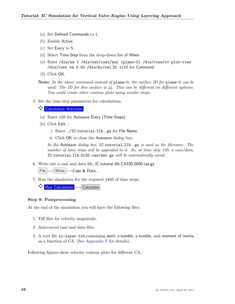
4. Set up commands to save figures for animations.

Calculation Activities (Execute Commands)−→ Create/Edit...



(a) Set Defined Commands to 1.

(b) Enable Active.

(c) Set Every to 5.

(d) Select Time-Step from the drop-down list of When.

(e) Enter /dis/sw 1 /dis/set/cont/sur (plane-0) /dis/view/rv plot-view/dis/cont vm 0 50 /dis/hc/vel %t.tiff for Command.

(f) Click OK.

Note: In the above command instead of plane-0, the surface ID for plane-0 can beused. The ID for this surface is 44. This can be different on different systems.You could create other contour plots using similar steps.

5. Set the time step parameters for calculations.

Calculation Activities

(a) Enter 120 for Autosave Every (Time Steps).

(b) Click Edit....

i. Enter ./IC tutorial IIb .gz for File Name.

ii. Click OK to close the Autosave dialog box.

In the Autosave dialog box, IC tutorial IIb .gz is used as the filename. Thenumber of time steps will be appended to it. So, at time step 120, a case/data,IC tutorial IIb 0120.cas/dat.gz will be automatically saved.

6. Write out a case and data file, IC tutorial IIb CA330 0000.cas.gz

File −→ Write −→Case & Data...

7. Run the simulation for the required 1400 of time steps.

Run Calculation −→ Calculate

Step 9: Postprocessing

At the end of the simulation you will have the following files:

1. Tiff files for velocity magnitude.

2. Auto-saved case and data files.

3. A text file ic-layer.txt,containing swirl, x-tumble, y-tumble, and moment of inertiaas a function of CA. (See Appendix F for details).

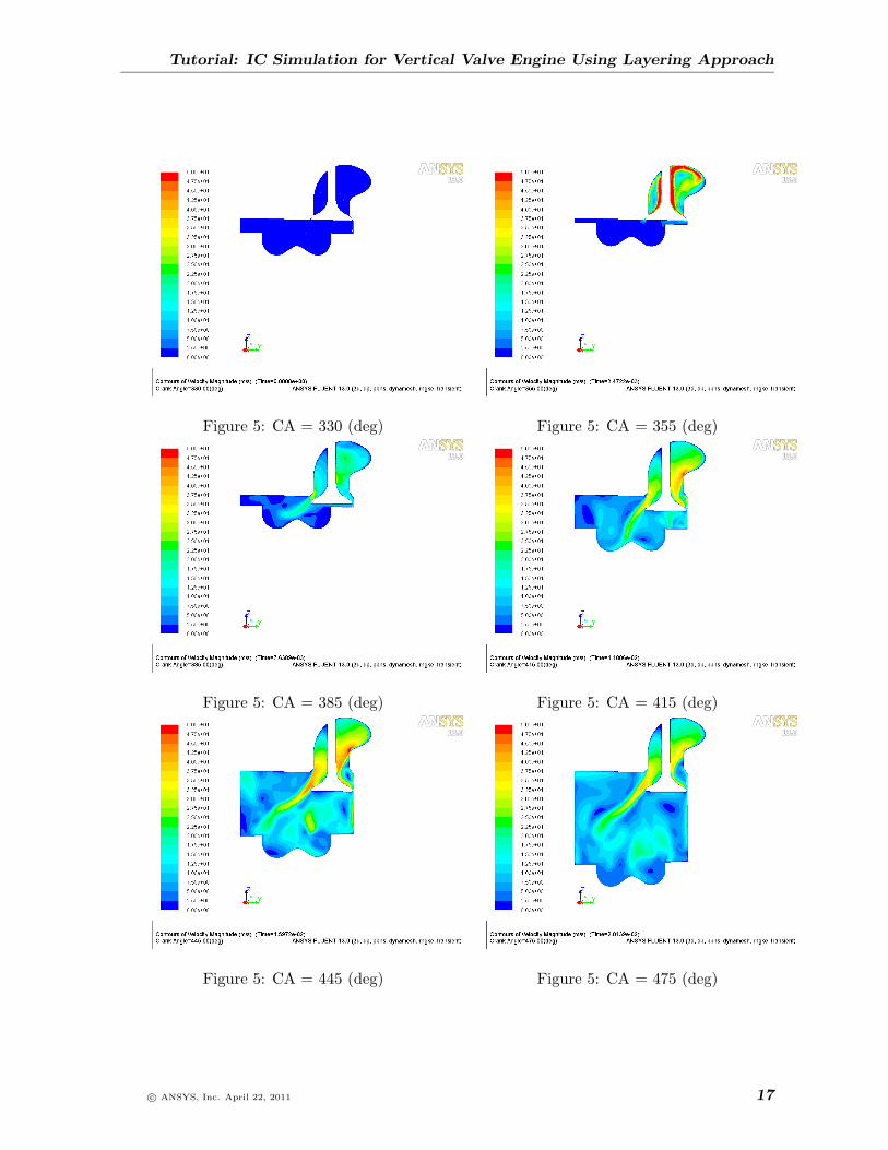
Following figures show velocity contour plots for different CA.



Figure 5: CA = 330 (deg) Figure 5: CA = 355 (deg)





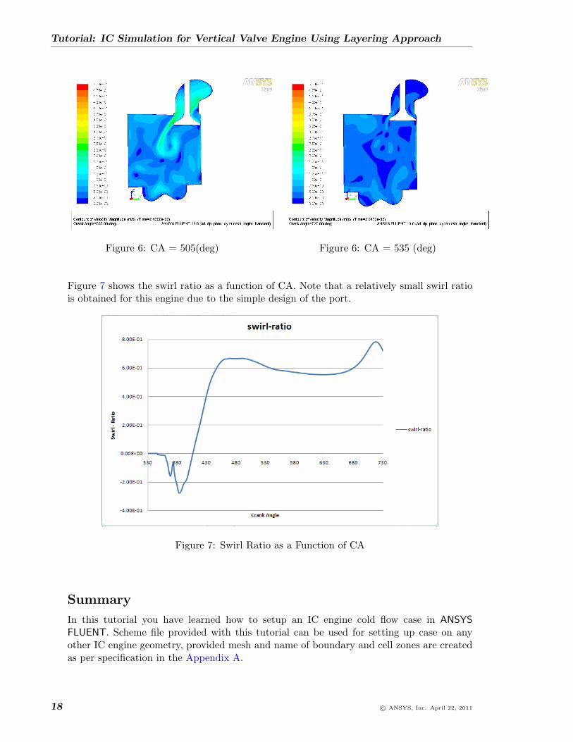
Figure 6: CA = 505(deg) Figure 6: CA = 535 (deg)

Figure 7 shows the swirl ratio as a function of CA. Note that a relatively small swirl ratiois obtained for this engine due to the simple design of the port.

Figure 7: Swirl Ratio as a Function of CA

Summary

In this tutorial you have learned how to setup an IC engine cold flow case in ANSYSFLUENT. Scheme file provided with this tutorial can be used for setting up case on anyother IC engine geometry, provided mesh and name of boundary and cell zones are createdas per specification in the Appendix A.



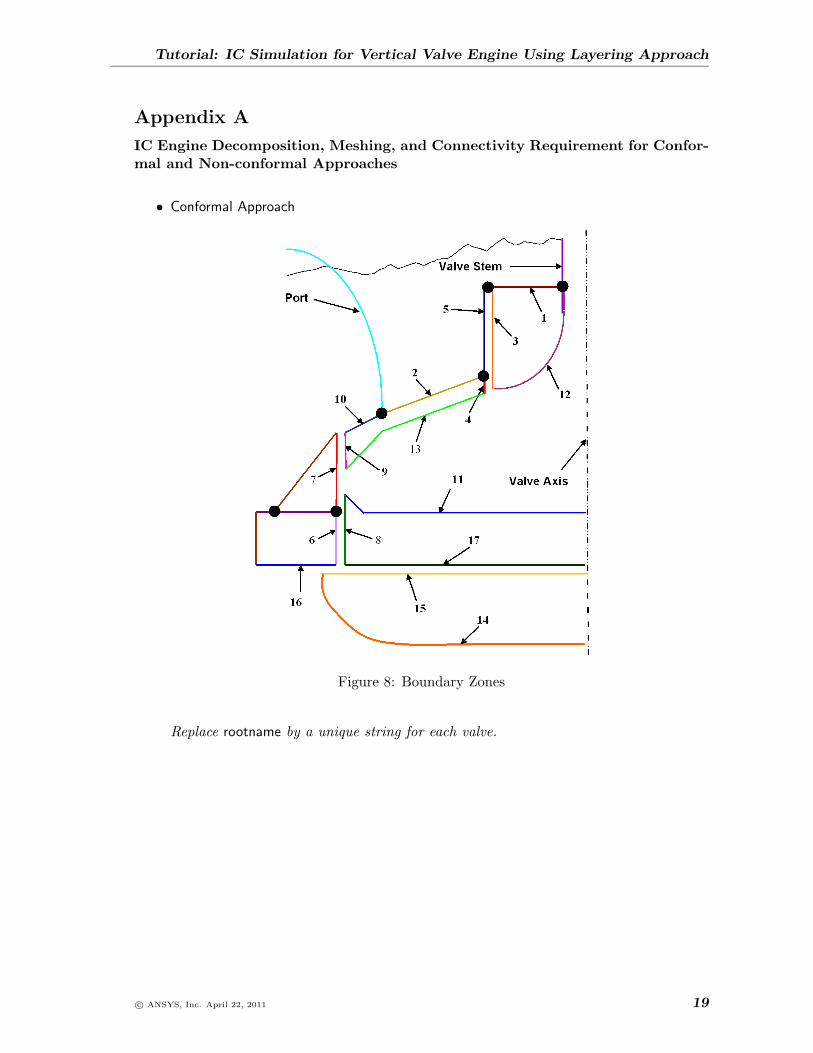
Appendix A

IC Engine Decomposition, Meshing, and Connectivity Requirement for Confor-mal and Non-conformal Approaches

• Conformal Approach

Figure 8: Boundary Zones

Replace rootname by a unique string for each valve.



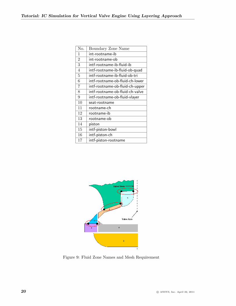
No. Boundary Zone Name1 int-rootname-ib

2 int-rootname-ob

3 intf-rootname-ib-fluid-ib

4 intf-rootname-ib-fluid-ob-quad

5 intf-rootname-ib-fluid-ob-tri

6 intf-rootname-ob-fluid-ch-lower

7 intf-rootname-ob-fluid-ch-upper

8 intf-rootname-ob-fluid-ch-valve

9 intf-rootname-ob-fluid-vlayer

10 seat-rootname

11 rootname-ch

12 rootname-ib

13 rootname-ob

14 piston

15 intf-piston-bowl

16 intf-piston-ch

17 intf-piston-rootname

Figure 9: Fluid Zone Names and Mesh Requirement



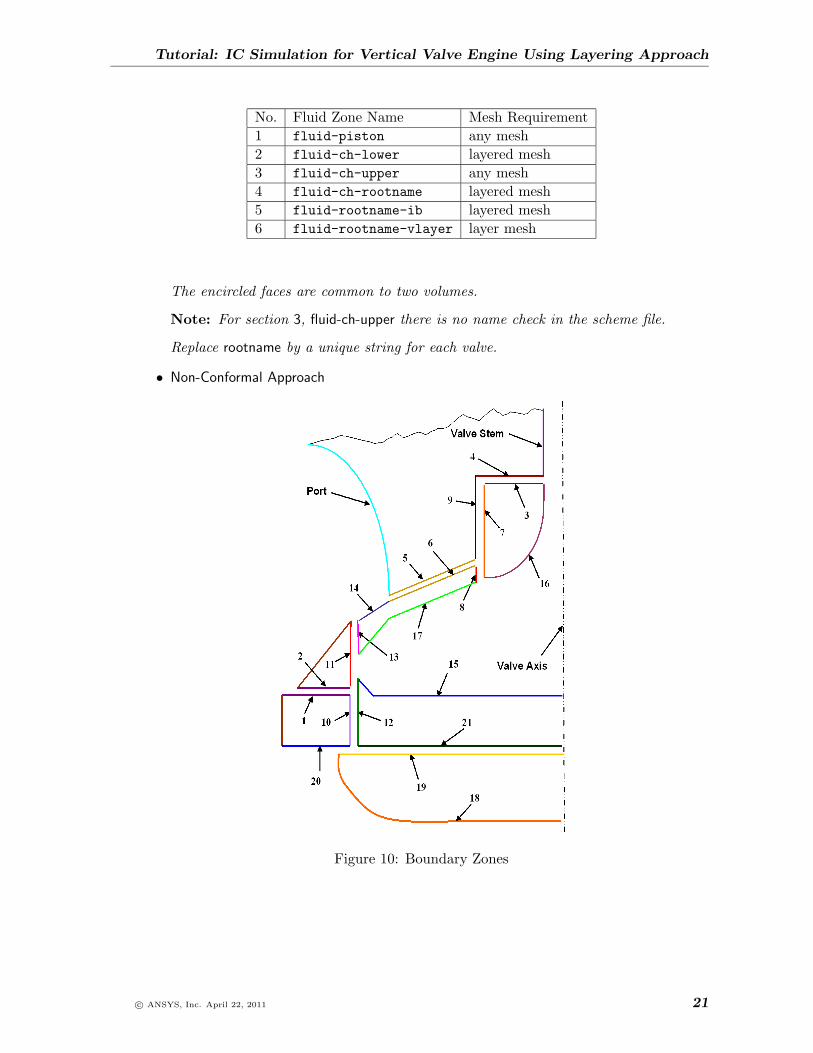
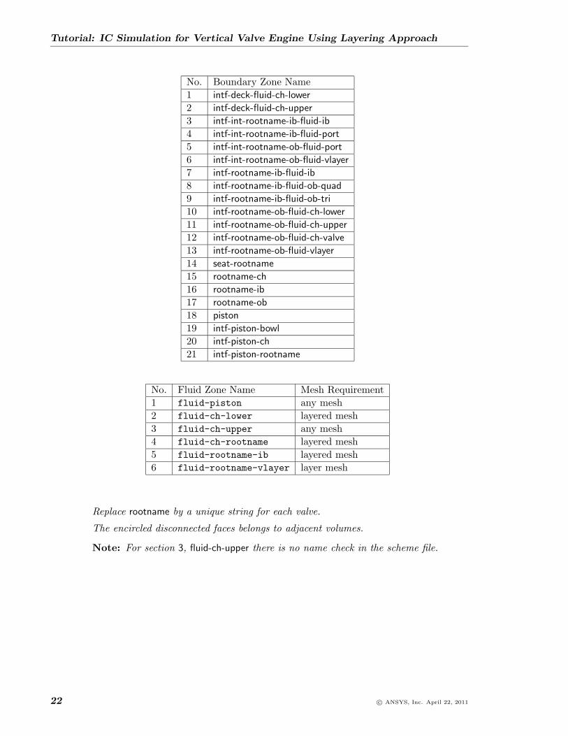
No. Fluid Zone Name Mesh Requirement1 fluid-piston any mesh2 fluid-ch-lower layered mesh3 fluid-ch-upper any mesh4 fluid-ch-rootname layered mesh5 fluid-rootname-ib layered mesh6 fluid-rootname-vlayer layer mesh

The encircled faces are common to two volumes.

Note: For section 3, fluid-ch-upper there is no name check in the scheme file.


• Non-Conformal Approach

Figure 10: Boundary Zones



No. Boundary Zone Name1 intf-deck-fluid-ch-lower

2 intf-deck-fluid-ch-upper

3 intf-int-rootname-ib-fluid-ib

4 intf-int-rootname-ib-fluid-port

5 intf-int-rootname-ob-fluid-port

6 intf-int-rootname-ob-fluid-vlayer

7 intf-rootname-ib-fluid-ib

8 intf-rootname-ib-fluid-ob-quad

9 intf-rootname-ib-fluid-ob-tri

10 intf-rootname-ob-fluid-ch-lower

11 intf-rootname-ob-fluid-ch-upper

12 intf-rootname-ob-fluid-ch-valve

13 intf-rootname-ob-fluid-vlayer

14 seat-rootname

15 rootname-ch

16 rootname-ib

17 rootname-ob

18 piston

19 intf-piston-bowl

20 intf-piston-ch

21 intf-piston-rootname

No. Fluid Zone Name Mesh Requirement1 fluid-piston any mesh2 fluid-ch-lower layered mesh3 fluid-ch-upper any mesh4 fluid-ch-rootname layered mesh5 fluid-rootname-ib layered mesh6 fluid-rootname-vlayer layer mesh


The encircled disconnected faces belongs to adjacent volumes.

Note: For section 3, fluid-ch-upper there is no name check in the scheme file.



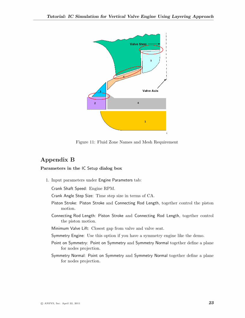
Figure 11: Fluid Zone Names and Mesh Requirement

Appendix B

Parameters in the IC Setup dialog box

1. Input parameters under Engine Parameters tab:

Crank Shaft Speed: Engine RPM.

Crank Angle Step Size: Time step size in terms of CA.

Piston Stroke: Piston Stroke and Connecting Rod Length, together control the pistonmotion.

Connecting Rod Length: Piston Stroke and Connecting Rod Length, together controlthe piston motion.

Minimum Valve Lift: Closest gap from valve and valve seat.

Symmetry Engine: Use this option if you have a symmetry engine like the demo.

Point on Symmetry: Point on Symmetry and Symmetry Normal together define a planefor nodes projection.

Symmetry Normal: Point on Symmetry and Symmetry Normal together define a planefor nodes projection.



2. Input Parameters under Piston Motion Setup tab:

Meshing Strategy Hybrid Approach: This approach is used for canted valve engine.Three different piston mesh types can be modeled under Hybrid Approach.For further details refer IC tutorial, IC Simulation for Canted Valve Engine UsingHybrid Approach.

Layering Approach: This approach is used for the vertical valve engine. There aretwo mesh types (conformal and non-conformal mesh type) used for layeringapproach.

Layering Setup Type: There are two different layering setup types; conformal and non-conformal approach. It depends on the decomposition of the geometry. ReferAppendix C for detailed information on the same. In the tutorial, conformalapproach is used.

Cylinder Axis Direction: Cylinder Axis Origin and Cylinder Axis Direction togetherdefine a cylinder for the engine cylinder. ANSYS FLUENT needs this to projectnodes on the engine cylinder back to a perfect cylinder.

3. Input parameters under Valve Motion Setup tab:

Number of Valves: The total number of vales in the engine.

Valve Number: Valve number for which parameters are setup.

For example, if there are total 4 valves, valve number parameter will vary from1 to 4. The parameters like Valve Name, Valve Profile Name, etc., are required tosetup for each valve number and these parameters are stored against the valvenumber.

Valve Name: The auto set up is done through name matching system. This is thevalve root name.

Valve Profile Name: Valve profile is used to define valve motion. This name is shownup on ANSYS FLUENT screen during the step of Read the Valve Profile.

Open Valve: CA to open the valve. At the specified CA, the valve will open by formingthe non-conformal interface.

Close Valve: CA to close the valve. At the specified CA, the valve will close by deletingthe non-conformal interface.

Refer Appendix D for the recommended practice to select the opening and closingcrank angles.

Valve Margin Radius: Valve radius.

Valve Axis Direction: Valve Axis Origin and Valve Axis Direction together define a cylin-der for the valve. ANSYS FLUENT needs this to project nodes back to a perfectcylinder.

Valve Axis Origin: Valve Axis Origin and Valve Axis Direction together define a cylinderfor the valve. ANSYS FLUENT needs this to project nodes back to a perfectcylinder.

Variable URFs: With this option enabled, the URFs are not a constant. When valvesare opening or closing, the URFs for k, e, Momentum, and Pressure will beautomatically reduced and later on switched back.



Variable Crank Angle Step Size: With this option enabled, the time step size is not aconstant. When valves are opening or closing, the time step size will be auto-matically reduced and later on switched back.

Duration: The duration for reduced URFs or/and time step size.

Appendix C

Conformal and Non-Conformal Approach

Conformal and non-conformal are the two different layering set up types in the pure layeringapproach. The difference between the two approaches is in the connectivity between differentvolumes. In conformal approach the volumes are connected to each other by a common face.Refer the Appendix A Figure 9 to find the connectivity between :

1. port volume and fluid-rootname-ib

2. port volume and fluid-rootname-vlayer

3. fluid-ch-upper and fluid-ch-lower

In the non-conformal approach these volumes are made disconnected and a mesh interfacewill be created between the adjacent faces of the two volumes.

It is possible to make the decomposition in conformal or non-conformal approach indepen-dent of the cylinder geometry.

With conformal approach, the port volume will be meshed with tetrahedral elements whilethe fluid-rootname-ib and fluid-rootname-vlayer will be meshed with hexahedral ele-ments. So when growing tetrahedral elements of port volume from the quad faces connectedto other volumes, there will be pyramid elements. It is undesirable to have pyramid elementsat high gradient regions in flow. This is one of the drawbacks of conformal approach.

A non-conformal approach removes the necessity of creating pyramid elements. This facili-tates the generation of a good quality tetrahedral mesh in the port region.

A non-conformal approach can also be useful when meshing is done by packages other thanGambit, where a conformal mesh is difficult to generate. With the non-conformal approachit should be taken care that the mesh density of the disconnected faces should be almostequal. This reduces the numerical errors due to the interpolation used for mesh interfaces.

Refer Appendix A Figure 8 and Figure 9 for detailed information of decomposition andmeshing to be followed in the conformal approach.

ReferAppendix A Figure 10 and Figure 11 for detailed information of decomposition andmeshing to be followed in the non-conformal approach.



Appendix D

Determining the valve opening and closing angles

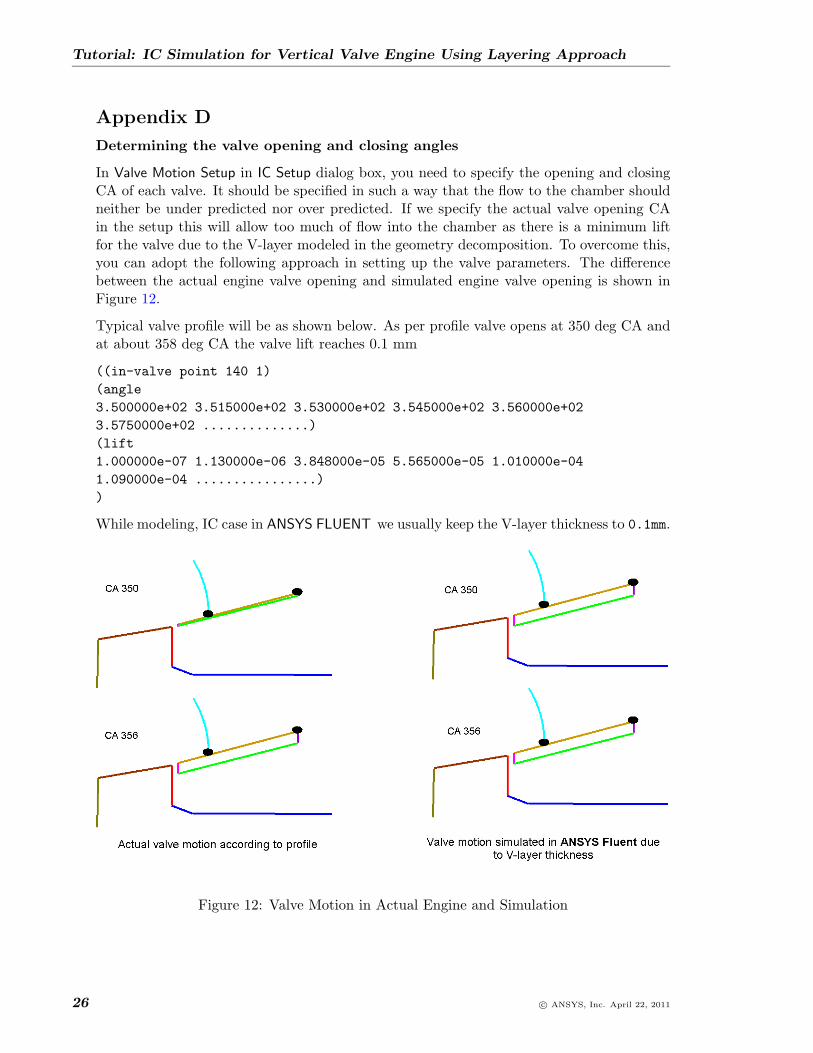
In Valve Motion Setup in IC Setup dialog box, you need to specify the opening and closingCA of each valve. It should be specified in such a way that the flow to the chamber shouldneither be under predicted nor over predicted. If we specify the actual valve opening CAin the setup this will allow too much of flow into the chamber as there is a minimum liftfor the valve due to the V-layer modeled in the geometry decomposition. To overcome this,you can adopt the following approach in setting up the valve parameters. The differencebetween the actual engine valve opening and simulated engine valve opening is shown inFigure 12.

Typical valve profile will be as shown below. As per profile valve opens at 350 deg CA andat about 358 deg CA the valve lift reaches 0.1 mm

((in-valve point 140 1)(angle3.500000e+02 3.515000e+02 3.530000e+02 3.545000e+02 3.560000e+023.5750000e+02 ..............)(lift1.000000e-07 1.130000e-06 3.848000e-05 5.565000e-05 1.010000e-041.090000e-04 ................))

While modeling, IC case in ANSYS FLUENT we usually keep the V-layer thickness to 0.1mm.

Figure 12: Valve Motion in Actual Engine and Simulation



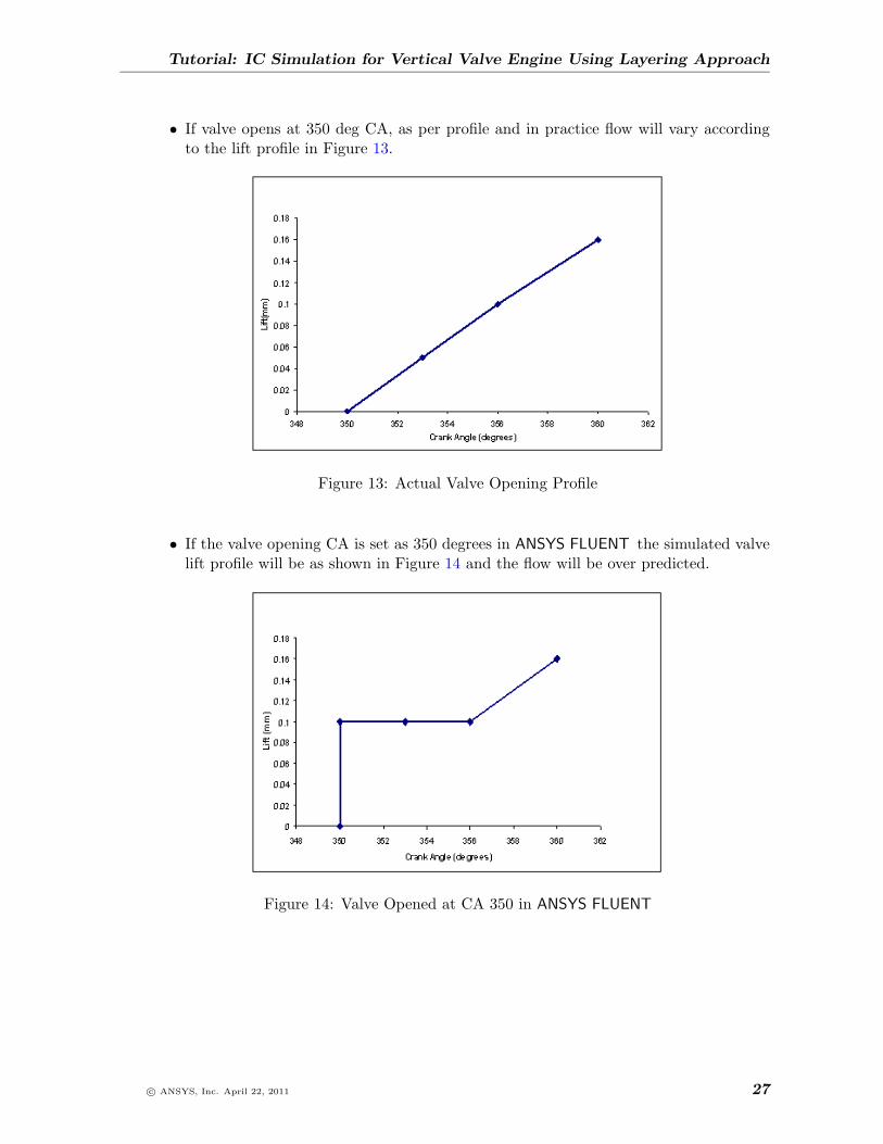
• If valve opens at 350 deg CA, as per profile and in practice flow will vary accordingto the lift profile in Figure 13.

Figure 13: Actual Valve Opening Profile

• If the valve opening CA is set as 350 degrees in ANSYS FLUENT the simulated valvelift profile will be as shown in Figure 14 and the flow will be over predicted.

Figure 14: Valve Opened at CA 350 in ANSYS FLUENT



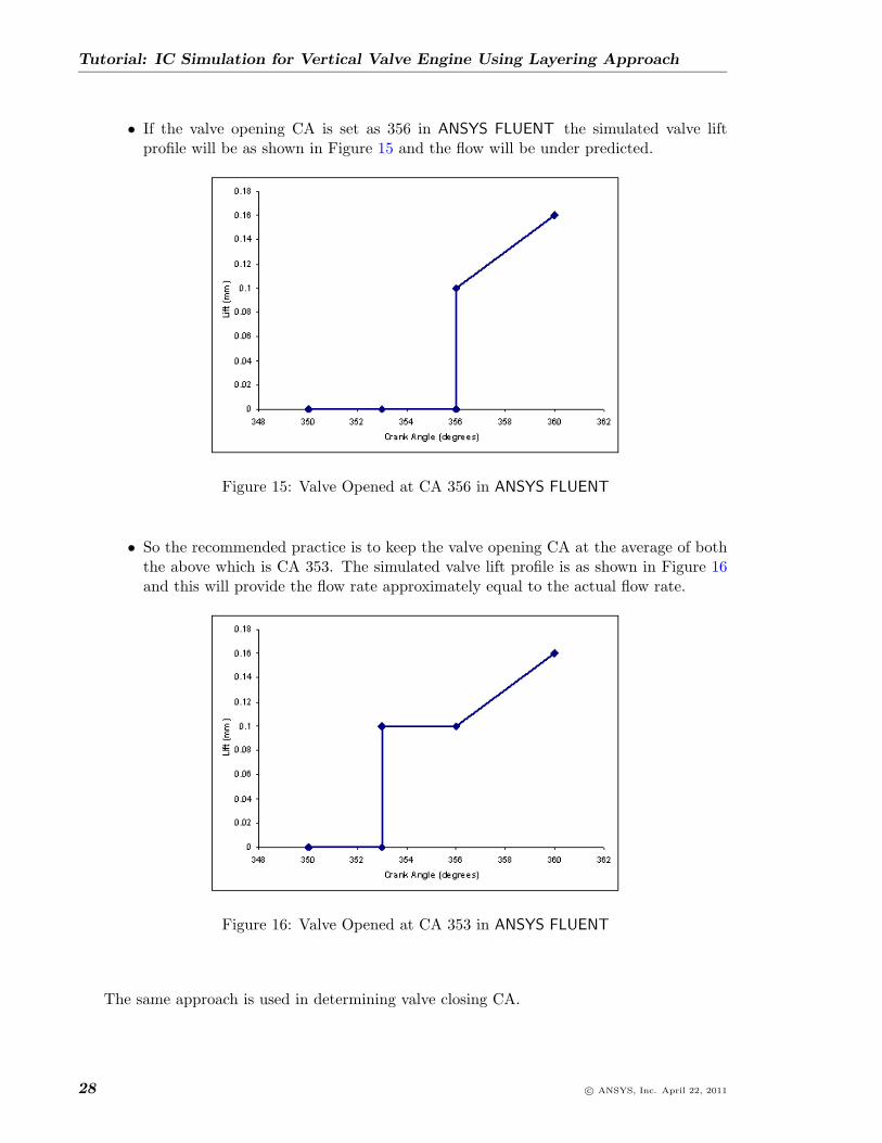
• If the valve opening CA is set as 356 in ANSYS FLUENT the simulated valve liftprofile will be as shown in Figure 15 and the flow will be under predicted.


• So the recommended practice is to keep the valve opening CA at the average of boththe above which is CA 353. The simulated valve lift profile is as shown in Figure 16and this will provide the flow rate approximately equal to the actual flow rate.


The same approach is used in determining valve closing CA.



Appendix E

Partitioning of Pure Layering IC Engines

IC engine simulation usually requires multiple processors due to high mesh count and com-plex physics. With using pure layering approach, it is recommended to do the parallelpartitioning in such a way that layering does not occur across the partition boundary. Forthe tutorial, engine cartesian x-coordinate is the recommended partition method.

Appendix F

Calculation of Swirl Ratio

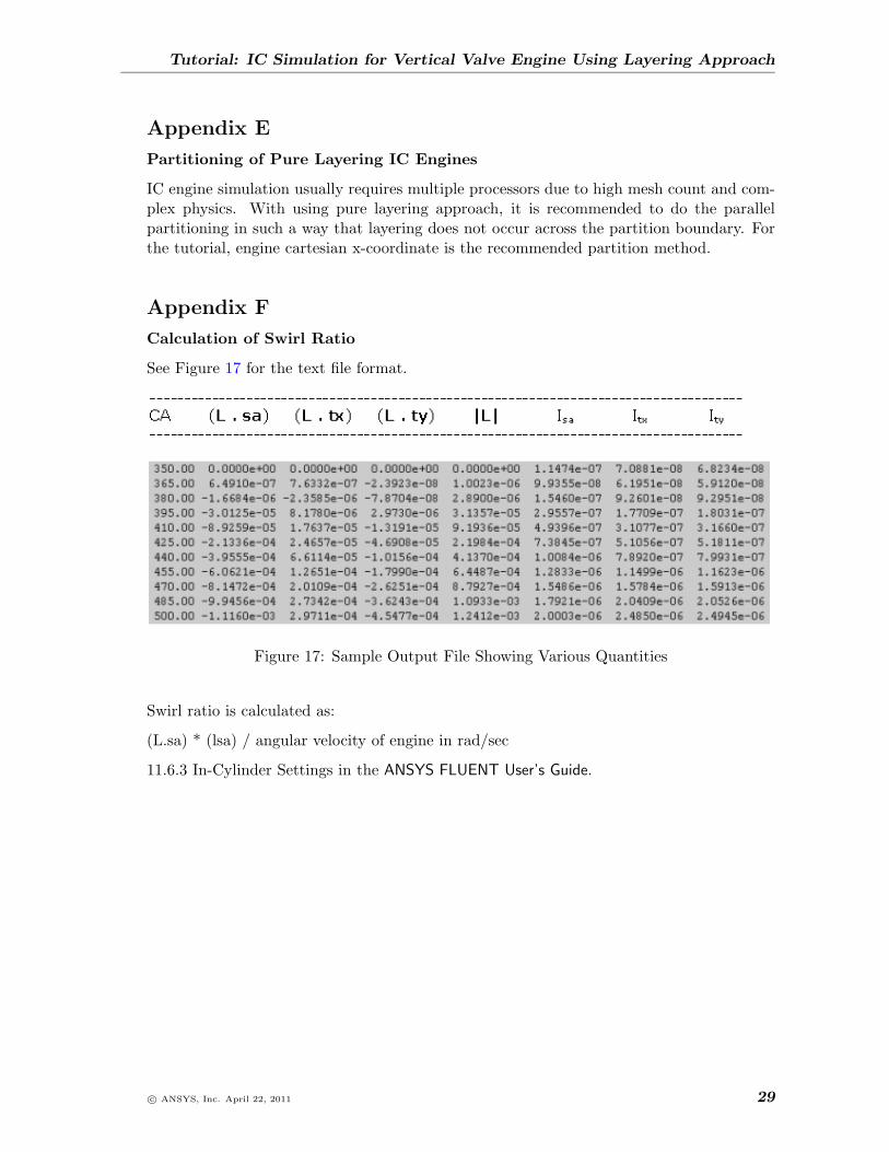
See Figure 17 for the text file format.

Figure 17: Sample Output File Showing Various Quantities

Swirl ratio is calculated as:

(L.sa) * (lsa) / angular velocity of engine in rad/sec

11.6.3 In-Cylinder Settings in the ANSYS FLUENT User’s Guide.


Documents

FLUENT IC Tut 02 Layering Approach