fluent-fsi_14.0_ws3_hyperelastic_flap_part1

© 2011 ANSYS, Inc. May 21, 20121 Release 14.0

14. 0 Release

Solving FSI Applications Using ANSYS Mechanical and ANSYS Fluent

Workshop 3 2-way FSI for a Hyperelastic Flap Including Dynamic Remeshing


Workshop Description:

This example considers the large deformation of a hyperelastic flap as a result of the hydrodynamic forces from a surrounding fluid flow. The flow is transient, and the coupling involves 2-way FSI between Fluent and Mechanical.

Learning Aims:

This workshop shows how to prepare a 2-way coupled Systems-Coupling solution in workbench. This includes:

– Setup of the Transient Structural case for the hyperelastic material.

– Setup of the Fluent dynamic-mesh case, including smoothing and re-meshing

– Setup and solution of the coupled flow case

Learning Objectives:

To understand all the key steps necessary for solving a full 2-way FSI simulation within Workbench that results in a large deformation which requires dynamic re-meshing.

Introduction


The fluid region is a channel 0.15 m high and 0.25 m long. Air enters at the left hand side at 20 m/s. This causes the flap, made of a hyperelastic rubber, to deform.

The simulation is run over 75 time steps. The solution is full 2-way FSI:• ANSYS Fluent transfers the pressure force on the flap to ANSYS Mechanical• ANSYS Mechanical computes the deformation, and transmits this to Fluent• Fluent modifies the mesh (using smoothing and re-meshing) to resolve the

motion

Note that system coupling must be a 3D analysis. In this case we will generate a mesh just 1 element/cell thick. The Fluent cells will be triangular prisms, but we can re-mesh these by using the ‘2.5D’ remeshing scheme.

Start, time =0 End, time = 0.0075s

Simulation to be performed


Starting Workbench

The geometry and mesh have already been created (both fluid and solid regions).

1. Start ANSYS Workbench (R14.0) and select File > Restore Archive:a) Select Hyperelastic_Flap.wbpzb) You will be asked for a Save As file name. Enter Hyperelastic_Flap.wbpj and

save to your working directory (save to a local hard disk, not a USB memory stick)

Parameters were used during the initial geometry creation (for controlling the top curve on the flap). This workshop will not be modifying these parameters, though you may wish to try this yourself later.


1. On the Workbench page, double-click on the Fluent Setup cell (B4)a) Keep default settings (3D, single precision, serial), click OK

2. In Fluent perform a mesh check (see image) and verify there are no warnings

3. Enable the Transient solver (see image)

4. Under Models, select Viscous and Edit. Select:a) k-epsilon (2-eqn)b) Realizable modelc) Enhanced Wall Treatmentd) Click OK

5. Under Materials, observe air is alreadyavailable by default

Fluent Setup - General


1. Select Boundary Conditions in the model tree

2. Observe that the following boundaries have defaulted to the correct type:a) Type symmetry for symmetry_1, symmetry_2b) Type wall for bottom_wall, top_wall,

wall_cfd_coupled

3. Click on inlet (type = velocity inlet) and select Edita) Set Velocity Magnitude to 20 m/s, Turbulence

Specification Method to Intensity and Hydraulic Diameter with 10% Turbulent Intensity and 0.2m Hydraulic Diameter.

b) Click OK

4. Click on outlet (type = pressure-outlet) and select Edita) Set Gauge Pressure to 0 Pa.b) Set the same turbulence specification the inlet

then click OK

Fluent Setup – Boundary Conditions


1. Select Dynamic Mesh in the model treea) Enable Dynamic Meshb) Enable Smoothing and Remeshingc) Select Settings

2. On the Smoothing tab, set the Method to Diffusiona) Set the Diffusion Function to boundary-distanceb) Set Diffusion Parameter to 1

3. Don’t close this panel yet

Diffusion smoothing works by diffusing the displacementsat moving boundaries into the domain. The boundary-distance function results in a high diffusivity nearboundaries (so the mesh near a boundary moves like arigid body) and a low diffusivity away from boundaries(so the mesh in the middle of a domain tends to deformto absorb the boundary motion.

Fluent Setup – Dynamic Mesh [1]


4. Go to the Remeshing tab and enable the2.5D method

5. Click on Mesh Scale Info and observe thecurrent maximum and minimum cell sizes

6. Enter values between these limits, so:a) Minimum Length Scale: 0.003 mb) Maximum Length Scale: 0.005 mc) Maximum Face Skewness: 0.7d) Size Remesh Interval: 1

7. Close the mesh-scale popup window, and click OK on theMesh Method Settings window

Fluent will normally only remesh either (in 2D) triangularcells, or (in 3D) tetrahedral cells. However in cases with aswept mesh like this, we can apply 2.5D remeshing so thatre-meshing is applied to the tri-prism grid cells



8. Under Dynamic Mesh Zones select Create/Edit

9. Select symmetry 1 from the Zone Names drop-down menu and set the Type to Deforming

a) On the Geometry Definition tab, set the Definition to plane

b) Set Point on Plane to [0, 0, 0.005]c) Set Plane Normal to [0, 0, 1]

d) On the Meshing Options tab disable the Smoothing and Remeshing toggles

10. Press Create

(Geometry Definition): Remember that Fluent does not have the underlying geometry for the model, it just sees the starting mesh. If we are to slide / move grid cells on this symmetry plane then Fluent needs to understand the geometric shape it is working with, in this case a plane. The symmetry plane mesh can now move, but it is constrained to the defined plane.(Meshing Options): For 2.5D re-meshing, one face will lead (in this case symmetry_2) and will have smoothing and re-meshing active. This face, symmetry_1 replicates the mesh of the lead face, and therefore we do not want smoothing and re-meshing active here.



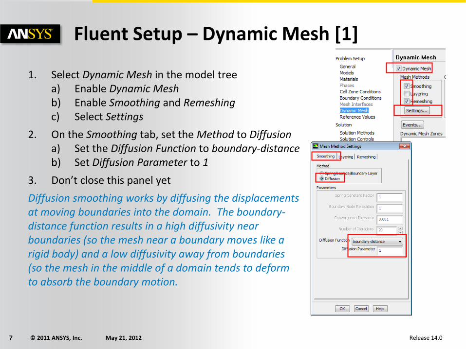
8. Select symmetry 2 from the Zone Names drop-down menu and set the Type to Deforming

13. For Geometry Definition, select planea) Set Point on Plane to [0, 0, 0]

(different than before)b) Set Plane Normal to [0, 0, 1]

14. Go to the Meshing Options tab and select:a) Smoothing: Onb) Remeshing: Onc) Minimum Length Scale: 0.003d) Maximum Length Scale: 0.005e) Maximum Skewness 0.7

15. Press Create



17. Select wall_cfd_coupled from the Zone Names menu and set the Type to System Coupling

18. Under Meshing Options, set the Cell Height to 0.003 m

19. Press Create

20. Close the Dynamic Mesh Zones panel

This is the key setting in Fluent to allow 2-way FSI

This boundary comprises the 3 surfaces (2 sides and top) of the flexible flap.

The deformed shape of this part is being computed by the finite-element code ANSYS Mechanical, and being transferred to Fluent. The deformation vector is defined for each individual node that makes up the coupled surface.



1. Back on the main Fluent model setup tree under Solution Methods set the Pressure-Velocity Coupling Scheme to Coupled

2. Under Solution Initialization select Hybrid Initialization then Initialize

3. Under Run Calculation enter 1 for the number of Time Steps (don’t press Calculate)

This value is not used, but must be greater than zero. We do not need to set the Time Step Size, this will be controlled externally from the System Coupling process.

4. Leave the number of iterations per time step set to 20

For System Coupling cases this is actually the number of Fluent iterations per Coupling Iteration

5. Save the project then close Fluent

Fluent Setup – General Solver Settings


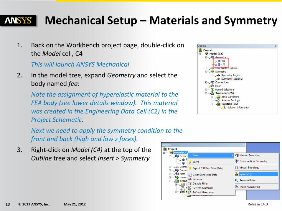
1. Back on the Workbench project page, double-click on the Model cell, C4

This will launch ANSYS Mechanical

2. In the model tree, expand Geometry and select the body named fea:

Note the assignment of hyperelastic material to the FEA body (see lower details window). This material was created in the Engineering Data Cell (C2) in the Project Schematic.

Next we need to apply the symmetry condition to the front and back (high and low z faces).

3. Right-click on Model (C4) at the top of theOutline tree and select Insert > Symmetry

Mechanical Setup – Materials and Symmetry


4. In the new Symmetry object (below Coordinate Systems) right-click and select Insert > Symmetry Regiona) Set Scoping Method to Named Selection then

from the drop-down list select symmetry_ab) Set Symmetry Normal to Z Axisc) Right click on this Symmetry Region in the model

tree and select Duplicated) Set the Named Selection to symmetry_b for the

Symmetry Region 2

Mechanical Setup – Materials and Symmetry


1. Right-click on Transient (C5) in the model tree and select Insert > Fixed Supporta) Set Scoping Method to Named Selectionb) Select clamped as the Named Selection

This is the small square face at the bottom of the flap that is rigidly fastened to the bottom of the channel

2. Right-click on Transient (C5) in the model tree and select Insert > Fluid Solid Interfacea) Set Scoping Method to Named Selectionb) Select wall_fea_coupled as the Named Selection

This is the key step for the Mechanical model in order to perform a 2-way FSI simulation. This surface is the wetted outer surface in contact with the fluid. System Coupling will map the forces from the CFD computation on to this surface, and transfer back the resulting deformation to Fluent.

Mechanical Setup – Support and Loads


1. Select Analysis Settings in the model treea) Set Auto Time Stepping to Offb) Set Define by to Substepsc) Enter Number Of Substeps as 1

A single substep is always recommended when using Mechanical with System Coupling

2. The Mechanical setup is now complete. Select File > Save Project, then close the Mechanical editor and return to Workbench

We do not need to set output controls here (these will be set in System Coupling later)

We do not need to set solution result quantities (stress / displacement) here, since the whole coupled model will be post-processed in CFD-Post

Mechanical Setup – Analysis Settings


1. On the Workbench Project Page drag a System Coupling (Component System) onto the Project Schematica) Draw a connector from the Fluent Setup cell (B4) to the System Coupling Setup

cell (D2)b) Draw a connector from the Transient Structural Setup cell (C5) to the System

Coupling Setup cell (D2)c) Note the Fluent Setup cell (B4) requests an update. Right-click and Updated) Note the Structural Setup cell (C5) requests an update. Right-click and Update

System Coupling Setup [1]


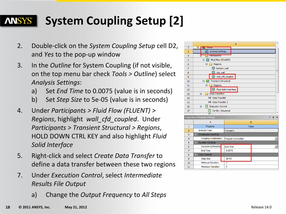
2. Double-click on the System Coupling Setup cell D2, and Yes to the pop-up window

3. In the Outline for System Coupling (if not visible, on the top menu bar check Tools > Outline) select Analysis Settings:a) Set End Time to 0.0075 (value is in seconds)b) Set Step Size to 5e-05 (value is in seconds)

4. Under Participants > Fluid Flow (FLUENT) > Regions, highlight wall_cfd_coupled. Under Participants > Transient Structural > Regions, HOLD DOWN CTRL KEY and also highlight Fluid Solid Interface

5. Right-click and select Create Data Transfer to define a data transfer between these two regions

7. Under Execution Control, select Intermediate Results File Output

a) Change the Output Frequency to All Steps



8. Save the project

When setting the time step size, the value (5e-05) will be given to both CFD and FEA codes (which is why we did not need to set this value in Fluent or Mechanical). We have kept the default Maximum Iteration of 5 in System Coupling. This is the maximum number of iterations System Coupling will perform between the participant solvers per time step. Hence within a given time step, we could find that:

• Fluent performs up to 20 flow iterations• Fluent passes the loads to Mechanical to compute the displacement• Mechanical performs iterations to converge its solution• Mechanical passes the new position back to Fluent

This whole process could then be repeated up to 5 times for each time step (in other words potentially 100 Fluent iterations per time step if convergence is poor).

Two new ‘Data Transfer’ objects have been added to the Model Tree. Data Transfer takes the force computed on Fluent (boundary ‘wall_cfd_coupled’) and transmits that to Transient Structural (boundary type ‘Fluid Solid Interface’). Data Transfer 2 takes the displacement from Transient Structural (boundary type ‘Fluid Solid Interface’) and transmits that to Fluent (boundary ‘wall_cfd_coupled’).



1. Before solving, make sure that View > Files is disabled in Workbench

The solution creates many results/backup files. Workbench is slow to display all these files after the solution. Ensuring the Files View is off allows you to quickly return to the Project page when the solution is finished

2. Click on Update Project in the main Workbench toolbar

Select each object under Solution Information to view the output transcript from the System Coupling, Fluent and Mechanical

Just before the main computation starts, it is important to check the Mapping Summary in the System Coupling output and see that 100% of the nodes have been paired up

System Coupling – Running the Simulation


2. Look at the System Coupling log file (click under Solution Information in the Outline):

a) Review the output. Note that typically the coupling system typically reaches convergence within 3 Coupling Iterations (so a maximum of 5 Coupling Iterations was appropriate)

3. Look at the Fluid Flow (FLUENT) log file:

a) See how in most cases convergence was reached on a given time step within less than the 20 iteration maximum, so this setting was appropriate

Note that if the Fluent UI remains open then the Fluent solution transcript will only appear in Fluent and not in System Coupling. Keeping Fluent open can be useful, for example to track monitor plots.

4. Look at the Transient Structural log file:a) See how in most cases force and displacement convergence was achieved

after 2 or 3 Equilibrium Iterations, which is good

As a guide, this will take about 15 mins to solve. You may want to stop the simulation early if short of time and carry on to post-processing.

System Coupling – Reviewing


1. Save the project

2. Select Return to Project, in the main Workbench toolbar

3. On the Project Schematic create a connection from the Transient StructuralSolution cell (C6) to the Fluent Results cell (B6)

Note that the 2 blocks may swap over (so Fluent becomes column ‘C’)

4. Double-click on the Fluent Results cell (C6) to launch CFD-Post

CFD-Post is able to read in the results data from both solvers to allow post-processing of both CFD and FEA data simultaneously

System Coupling – Post-processing

Documents

fluent-fsi_14.0_ws3_hyperelastic_flap_part1