Embed Size (px)
Citation preview
FLUE GAS DESULFURIZATION: COST AND FUNCTIONALANALYSIS OF LARGE SCALE PROVEN PLANTS
by
Mr. Jean Tilly
,..Sc. Thesis, Chemical Engineering Dept.
Massachusetts Institute of Technology, Cambridge, MA 02139and
Energy Laboratory Report No. MIT-EL 33-006
June 1983
*II 1, 1111 I ,1I IEY9 14111E10, 11 1
-2-
FLUE GAS DESULFURIZATION:
COST AND FUNCTIONAL ANALYSIS OF LARGE - SCALE AND PROVEN PLANTS
by
Jean Tilly
Submitted to the Department of Chemical Engineering
on May 6, 1983
in partial fullfillment of the requirements for the degree of
Master of Science in Technology and Policy
ABSTRACT
Flue Gas Desulfurization is a method of controlling the emission ofsulfurs, which causes the acid rain. The following study is based on 26utilities which burn coal, have a generating capacity of at least 50Megawatts (MW) and whose Flue Gas Desulfurization devices have beenoperating for at least 5 years. An analysis is made of the capital andannual costs of these systems using a comparison of four main processes:lime, limestone, dual alkali and sodium carbonate scrubbing. Thefunctional analysis, based on operability, allows a readjustment of theannual costs and a determination of the main reasons for failure. Finallyfour detailed case studies are analyzed and show the evolution of cost andoperability along the years.
Thesis Supervisor: Dr. Dan Golomb
Title: Visiting Scientist
- 01110 1 1,iiiii1mlonl
-3-
ACKNOWLEDGEMENT a
I would like to express my sincere thanks to Dr. Dan Golomb for his
guidance, support and contribution to this thesis. I have very much
appreciated working with him.
I also want to thank Jane Schneckenburger for the time and care she
took in correcting and editing this thesis.
Finally, Alice Giubellini is greatfully acknowledged for the fine job
she did at typing the manuscript.
MUNlNIMMMM IU1011i
-4-
TABLE OF CONTENTS
Section 1 Introduction
1.1 Origin and Consequences of "Acid Rain" . . . .
1.1.1 Origin of "Acid Rain" . . . . . . . . ...
1.1.2 Consequences of "Acid Rain" . . . . . .
1.2 Survey of the Different Methods of Control . ...
1.2.1 Liming . ........... ......
1.2.2 Coal Washing ......... . . . . ..
1.3 Definition of the Flue Gas Desulfurization (FGD) .
1.4 Objectives ................... ..
1.5 Method of Approach ......... . . ...
Section 2 Technical Background
2.1 Introduction ..... .... . . . . . . . . . .
2.2 FGD Growth Trends . . . . . . . . . . . . . . . .
2.3 Limestone Scrubbing . . . . . . . . . . . . . . .
2.3.1 Process Description . . . . . . . . . . . .
2.3.2 Process Chemistry . . . . . . . . . . . . .
2.3.3 Description of Equipment Components . ...
2.3.4 Advantages and Disadvantages . . . . . . . .
2.4 Lime Scrubbing . . . . . . . . . . . . . . . ...
2.4.1 Process Description . . . . . . . . . ...
2.4.2 Process Chemistry . . . . . . . . . . . ..
2.4.3 Description of Equipment Components . ...
2.4.4 Advantages and Disadvantages . . . . .
,
. . . . . 20
. . . . . 20
. . . . . . 25
. . . . . 25
. . . . . 25
.. . . . 28
. . . . . . 32
. . . . . . 33
. . . . . . 33
. . . . . . 33
. . .... 35
. . . . . . . . . 35
11 14,11 I IM 0
-5-
2.5 Dual Alkali Scrubbing . . . . . . . . . .
2.5.1 Process Description . . . . . . . .
2.5.2 Process Chemistry . . . . . . . . .
2.5.3 Description of Equipment Components
2.5.4 Advantages and Disadvantages ....
2.6 Sodium Carbonate Scrubbing . .......
2.6.1 Process Description . . . . . . . .
2.6.2 Process Chemistry . . . . . . . . .
2.6.3 Description of Equipment Components
2.6.4 Advantages and Disadvantages . ...
Section 3 Cost Analysis of Proven FGD
3.1 Introduction . ..... ... .. . ...
3.2 Description of the Methodology . . . . . .
3.2.1 Collection of the Data . ......
3.2.2 Description of Cost Elements . . . .
3.2.3 Cost Adjustment Procedure . . . . .
3.3 Results and Interpretation . .......
3.3.1 Introduction ...........
3.3.2 Capital and Annual Costs . .....
3.3.3 Energy Consumption . ........
3.3.4 Impact on Consumer/Producer . . . .
3.3.5 Combination of Annual and Capital Coor Net Present Value
3.3.6 Conclusion . ............
. . . . . . . . . . 36
. . . . . . . . . . 36
. . . . . . . . . . 37
40
. . . . . . . . . . 41
. . . . . . . . . . 42
. . . . . . . . . . 42
. . . . . . . . . . 42
. . . . . . . . . . 44
. . . . . . . . . . 44
. . . . . . . . . . 45
. . . . . . . . . . 46
. . . . . . . . . . 46
. . . . . . . . . . 46
. . . . . . . . . . 47
. . . . . . . . . . 48
. . . . . . . . . . 48
. . . . . . . . . . 50
.... . . . . . . 55
. . . . . . . . . . 58
sts . . . .. ... 59
. . . . . 63. .
Section 4 Functional Analysis of Proven FGD
4.1 Introduction . . . . . . . . . . . . * . . . . . .
4.2 Description of the Methodology . . . . . . . . .
4.2.1 Definition of Different Viability Indexes . .
4.2.2 Collection of the Data . . . . . . . . . . .
4.3 Results and Interpretation . . . . .. ...........
4.3.1 Comparison of the Different Viability Indexesin 1980 or 1981
4.3.2 Evolution of the Operability . . . . . . .
4.3.3 Regulatory Classes and Operability Limit . . .
4.3.4 Main Reasons for Failure . . . . . . . .
4.3.5 Other Performance Indexes . .. .........
4.4 Relation between Operability and Cost . . . .
4.4.1 Definition of the Operating Cost . . ...
4.4.2 Average Cost Curve . . . . . . . . .
4.5 Conclusion
Section 5 Case Studies
5.1 Introduction
5.2 New Lime Scrubbing, Conesville 5 .
5.2.1 Evolution of the Operability ..
5.2.2 Evolution of the Cost . . .
5.2.3 Problems Encountered . . . .
5.3 New Limestone Scrubbing, Duck Creek 1
5.3.1 Evolution of the Operability .
5.3.2 Evolution of the Cost . . .
5.3.3 Problems Encountered .....
. . . . . 65
. . . . . 66
. . . . . 66
. . . . . 68
. . . . . 69
. . . . . 69
. . . . . 78
..... 81
. . . . . 85
. . . . . 87
. . . . . 90
. . . . . 90
. . . . . 93
. . . . . 99
. . S
S . . .
S S
. ~ S
. . S S
101
102
102
103
104
106
106
107
108
---- 1--rr lll III l I ,
-6-
,i8MMArIi
S . . . . . . . . . . . . . . . . . . .
5.4 Retrofit Lime Scrubbing, Cane Run 4
5.4.1 Evolution of the Operability
5.4.2 Evolution of the Cost . . ..
5.4.3 Problems Encountered . . . . .
5.5 Retrofit Limestone Scrubbing, Cholla
5.5.1 Evolution of the Operability .
5.5.2 Evolution of the Cost . . ..
5.5.3 Problems Encountered . . . ..
. . . . . . . . . . . .
. . . . . . . . . . . .
. . . . . . . . . . . .
. . . . . . . . . . . .
1 . . . . . . . . . .
. . . . . . . . . . . .
. . . . . . . . . . . .
. . . . . . . . . . . .
5.6 Conclusion . . . . .
Section 6 Conclusions and
6.1 Conclusions . . . .
6.2 Recommendations . .
Appendix . . . . . . . .
Definition of the Average
Recommendations
120
121
and of the Standard
123
123Deviation
References . . . . . . . . . . . . . . . . . . . . . . . . .
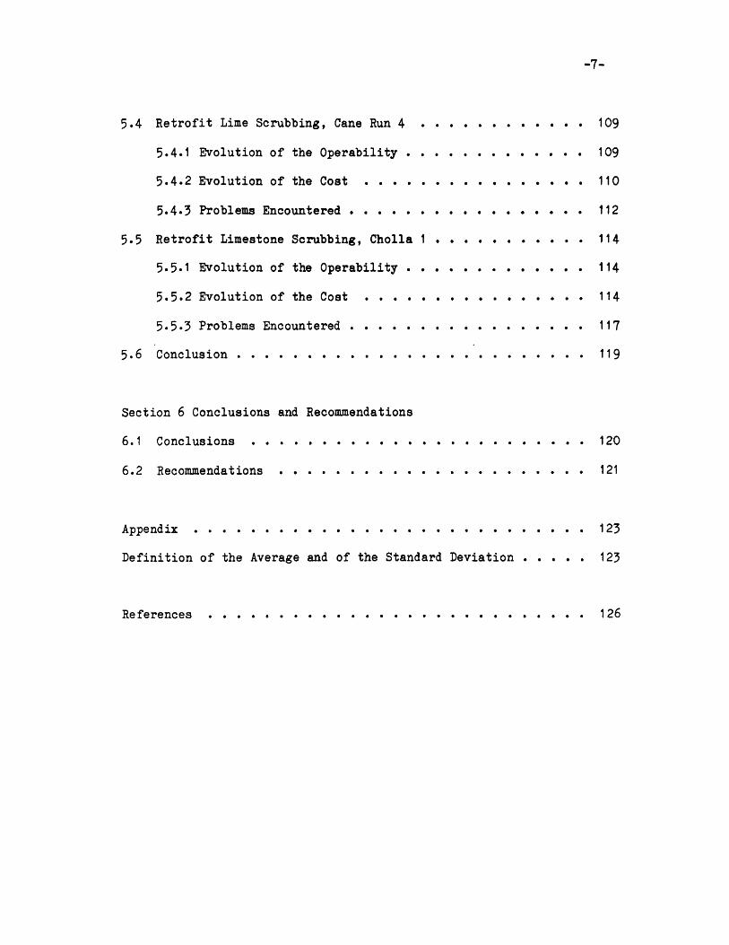
-7-
109
109
110
112
114
114
114
117
119. . . * . . . .
. . . . * . . . . .
126
-8-
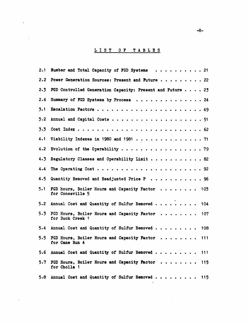
LIST OF TABLES
Number and Total Capacity of FGD Systems . . . .
Power Generation Sources: Present and Future .....
FGD Controlled Generation Capacity: Present and Future
S. . . 21
S. . . 22
S. . . 23
2.4 Summary of FGD Systems by Process . .
3.1 Escalation Factors . . .. ..
3.2 Annual and Capital Costs . . . . . . . . . .
3.3 Cost Index . . . . . . . . . . . . . . . . .
4.1 Viability Indexes in 1980 and 1981 . . . . .
4.2 Evolution of the Operability . . . . .
4.3 Regulatory Classes and Operability Limit
4.4 The Operating Cost . . . . . . . . . .
4.5 Quantity Removed and Readjusted Price P
5.1 FGD hours, Boiler Hours and Capacity Factorfor Conesville 5
5.2 Annual Cost and Quantity of Sulfur Removed .
5.3 FGD Hours, Boiler Hours and Capacity Factorfor Duck Creek 1
5.4 Annual Cost and Quantity of Sulfur Removed .
5.5 FGD Hours, Boiler Hours and Capacity Factorfor Cane Run 4
5.6 Annual Cost and Quantity of Sulfur Removed .
5.7 FGD Hours, Boiler Hours and Capacity Factorfor Cholla 1
5.8 Annual Cost and Quantity of Sulfur Removed .
. . . . . .
. . . . . .
. . . . . .
2.1
2.2
2.3
.. . . . . . . . 24
. . . . . . . . . 49
. . . . . . . . . 51
.... . . . . . 62
. . . .. . . 71
. . . . . . . . . 79
.... . . . . . 82
. . . . . . . . . 92
.... . . . . . 96
. . . . . . . 103
104
107
108
111
111
115
115
MM Mwilllfil 11411 1 Miiimll mm
-9-
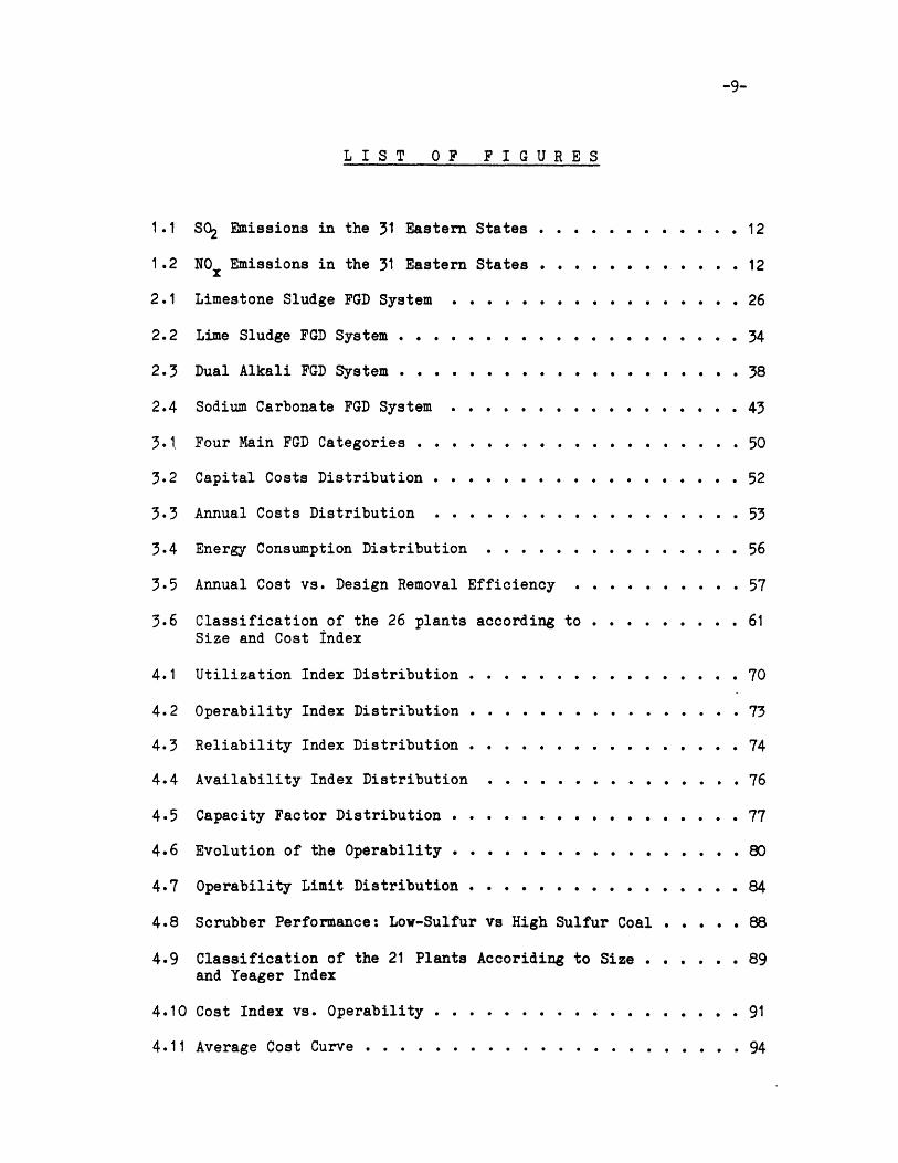
LIST OF FIGURES
1.1 S02 Emissions in the 31 Eastern States .
1.2 NOx Emissions in the 31 Eastern States .
2.1 Limestone Sludge FGD System . . . . . . .
2.2 Lime Sludge FGD System . . . . . . . . . .
2.3 Dual Alkali FGD System . . . . . . . . . .
2.4 Sodium Carbonate FGD System . . . . . . .
3.1 Four Main FGD Categories . . . . . . . . .
3.2 Capital Costs Distribution . . . . . . . .
3.3 Annual Costs Distribution . . . . . . . .
3.4 Energy Consumption Distribution . . . . .
3.5 Annual Cost vs. Design Removal Efficiency
3.6 Classification of the 26 plants accordingSize and Cost Index
4.1 Utilization Index Distribution . . . . . .
4.2 Operability Index Distribution . . . . . .
4.3 Reliability Index Distribution . . . . . .
4.4 Availability Index Distribution . . . . .
4.5 Capacity Factor Distribution . . . . . . .
4.6 Evolution of the Operability . . . . . . .
4.7 Operability Limit Distribution . . . . . .
4.8 Scrubber Performance: Low-Sulfur vs High Sulfur Coal
4.9 Classification of the 21 Plants Accoriding to Sizeand Yeager Index
4.10 Cost Index vs. Operability . . . . . . . . . . . . .
4.11 Average Cost Curve . . . . . . . . . . . . . . . . .
S. . . . 89
. . . . . 91
..... 94
...... . . . 12
.. .......... 12
.. .......... 26
. . . . ....... 34
. . . .. .......... . 38
. . . .. .. .......... 43
. . . .. .. .......... 50
. . . . .. .. .......... 52
. . . .. .. .......... 53
. . . .. .. .......... 56
. . . .. .. .......... 57
to . . . . . . . . . 61
.. . .. .......... 70
. . . .. .. .......... 73
. . . .. .. .......... 74
. . . .. .. .......... 76
. .......... 780
. . . . . . . . 84

-10-
5.1 Evolution of the Operability Conesville 5 . ........ 102
5.2 Evolution of the Operability Duck Creek 1 . . . . .. . . . 106
5.3 Evolution of the Operability Cane Run 4 . . .......... 110
5.4 Evolution of the Operability Cholla 1 . . . . . . ... 114
5.5 Case Studies Average Cost Curves . . . . . .. ....... 116
-11-
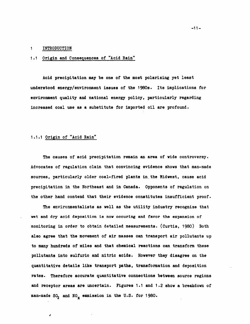
1 INTRODUCTION
1.1 Origin and Consequences of "Acid Rain"
Acid precipitation may be one of the most polarizing yet least
understood energy/environment issues of the 1980s. Its implications for
environment quality and national energy policy, particularly regarding
increased coal use as a substitute for imported oil are profound.
1.1.1 Origin of "Acid Rain"
The causes of acid precipitation remain an area of wide controversy.
Advocates of regulation claim that convincing evidence shows that man-made
sources, particularly older coal-fired plants in.the Midwest, cause acid
precipitation in the Northeast and in Canada. Opponents of regulation on
the other hand contend that their evidence constitutes insufficient proof.
The environmentalists as well as the utility industry recognize that
wet and dry acid deposition is now occuring and favor the expansion of
monitoring in order to obtain detailed measurements. (Curtis, 1980) Both
also agree that the movement of air masses can transport air pollutants up
to many hundreds of miles and that chemical reactions can transform these
pollutants into sulfuric and nitric acids. However they disagree on the
quantitative details like transport paths, transformation and deposition
rates. Therefore accurate quantitative connections between source regions
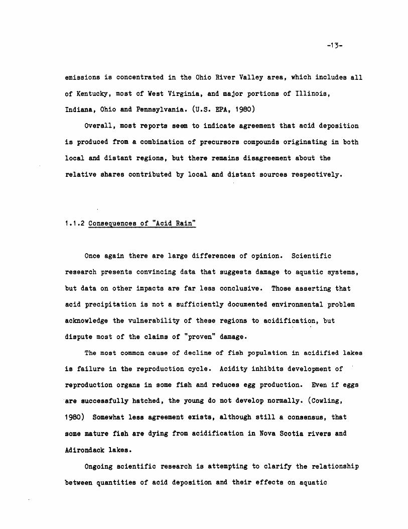
and receptor areas are uncertain. Figures 1.1 and 1.2 show a breakdown of
man-made SQ2 and NOx emission in the U.S. for 1980.
,01' Eli 1 109--
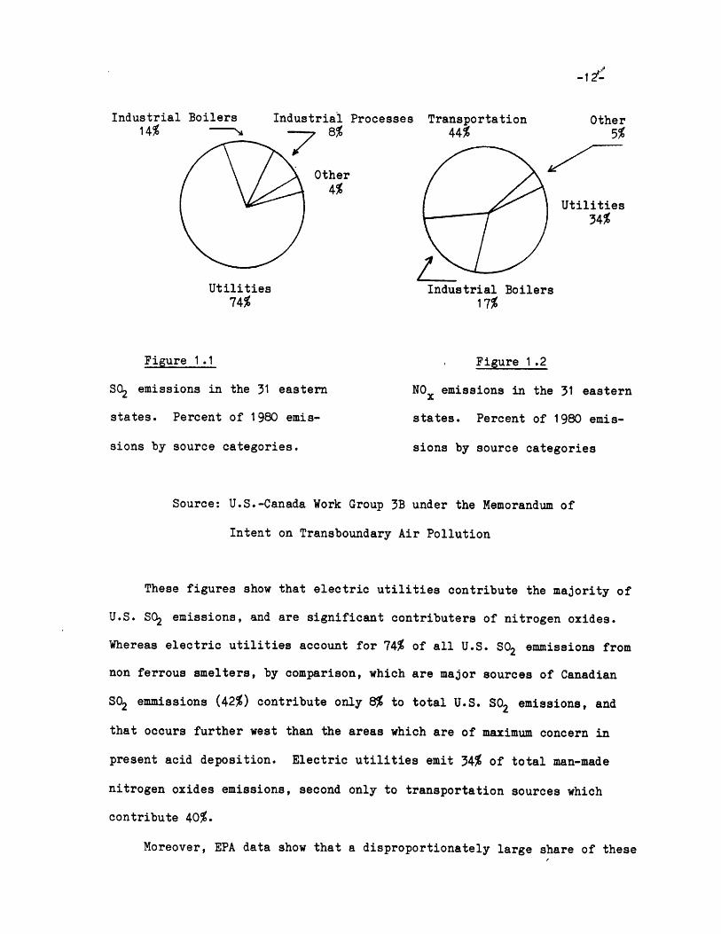
-12cIndustrial Boilers
14% ---Industrial Processes Transportation
8% 44%
Other4%
Other5%
Utilities34%
Utilities74%
Figure 1 .1
SO2 emissions in the 31 eastern
states. Percent of 1980 emis-
sions by source categories.
Industrial Boilers17%
Figure 1.2
NOx emissions in the 31 eastern
states. Percent of 1980 emis-
sions by source categories
Source: U.S.-Canada Work Group 3B under the Memorandum of
Intent on Transboundary Air Pollution
These figures show that electric utilities contribute the majority of
U.S. SO2 emissions, and are significant contributers of nitrogen oxides.
Whereas electric utilities account for 74% of all U.S. S02 emmissions from
non ferrous smelters, by comparison, which are major sources of Canadian
SO2 emmissions (42%) contribute only 8% to total U.S. S02 emissions, and
that occurs further west than the areas which are of maximum concern in
present acid deposition. Electric utilities emit 34% of total man-made
nitrogen oxides emissions, second only to transportation sources which
contribute 40%.
Moreover, EPA data show that a disproportionately large share of these
-1 3-
emissions is concentrated in the Ohio River Valley area, which includes all
of Kentucky, most of West Virginia, and major portions of Illinois,
Indiana, Ohio and Pennsylvania. (U.S. EPA, 1980)
Overall, most reports seem to indicate agreement that acid deposition
is produced from a combination of precursors compounds originating in both
local and distant regions, but there remains disagreement about the
relative shares contributed by local and distant sources respectively.
1.1.2 Consequences of "Acid Rain"
Once again there are large differences of opinion. Scientific
research presents convincing data that suggests damage to aquatic systems,
but data on other impacts are far less conclusive. Those asserting that
acid precipitation is not a sufficiently documented environmental problem
acknowledge the vulnerability of these regions to acidification, but
dispute most of the claims of "proven" damage.
The most common cause of decline of fish population in acidified lakes
is failure in the reproduction cycle. Acidity inhibits development of
reproduction organs in some fish and reduces egg production. Even if eggs
are successfully hatched, the young do not develop normally. (Cowling,
1980) Somewhat less agreement exists, although still a consensus, that
some mature fish are dying from acidification in Nova Scotia rivers and
Adirondack lakes.
Ongoing scientific research is attempting to clarify the relationship
between quantities of acid deposition and their effects on aquatic
-14-
ecosystems. This research will help the scientist to predict
quantitatively how much damage to aquatic ecosystems can be expected in the
future from acid deposition and therefore to estimate thresholds or
tolerance levels of acid deposition.
Environmental impacts other than those on aquatic ecosystems are very
difficult to quantify. Acid precipitation could cause damage to plant
tissues and interfere with photosynthesis. It could also stunt forest
growth and reduce yields of tomatoes, beans and other agricultural crops.
Acid precipitation is also suspected to corrode buildings and statues
(U.S. EPA, 1980) and to have indirect health effects. Metals such as lead
or mercury can be dissolved and carried by water of greater than usual
acidity and contaminate fish or drinking water.
1.2 Survey of the Different Methods of Control
Control strategies proposed to deal with acid precipitation vary
substantially in their costs, energy consumption and ability to reduce
emissions. The least expensive strategies-such as liming lakes and streams
or coal washing- offer the smallest potential for reducing impacts, while
the most expensive strategies-such as retrofitting scrubbers onto older
existing power plants-reduce emissions the most. A short description of
liming and coal washing follows. Scrubbing is discussed with more detail
in Section 1.3 and Section 2.
-15-
1.2.1 Liming
Liming is the use of limestone (calcium carbonate) or other alkaline
materials to neutralize the excess acid in lakes, streams, or ponds.
Unlike many other control methods, it would deal with all sorts of acids
rather than sulfuric acid only. However it would not solve the alleged
impacts of acid precipitation on terrestrial ecosystems.
Ontario's Ministry of Environment reports having successfully restored
the pH of four acidified lakes near the Province's Sudbury smelters to
normal, at a cost of about $50 per acre. However the effects are temporary
(usually three to four years) and it can only be applied in about one
percent of the cases for economic and logistic reasons. (e.g. difficult
access to the lakes).
.1.2.2 Coal Washing
Coal washing is viewed as a relatively inexpensive technique to make
moderate reductions of Sq emissions. it is a process that removes pyritic
sulfur from coal before it is burned, and is most effective when used with
high sulfur coals such as those in northern Appalachia and the Midwest.
Coal washing can reduce sulfur content of Pennsylvania and Illinois coals
by over 30 percent. (Chapman, et., al., 1981)
Cleaning all coals for the eight eastern and midwestern states would
increase the average delivered cost of raw coal by only 10 to 20 percent.
Capital and annual costs of 200 million tons per year coal washing program
.'illillffillill Ili m m m11 1,, m
-16-
would be $3 billion and $1 billion, respectively.
Coal washing's major drawback is its limited potential for sulfur
removal. If 10 to 30 percent sulfur removal is deemed sufficient to
mitigate acid precipitation, then it migh be a cost-effective strategy. If
however, greater S0 reductions are warranted, then coal washing will not
suffice.
1.3 Definition of Flue Gas Desulfurization (FGD)
Flue Gas Desulfurization takes place in a complex, large-scale
chemical reactor which is located between the combustion chamber and the
smokestack. The combustion products (flue gases) are exposed to a lime or
limestone slurry that is sprayed in their path. Sulfur dioxid in the gas
reacts with the spray and goes into solution, from which it is later
removed, dewatered and extruded in the form of sludge.
FGD processes can be best categorized by process (i.e. wet or dry,
lime, limestone, dual alkaii, sodium carbonate, etc.). FGD processes can
also be categorized by the manner in which the sulfur compounds removed
from the flue gases are eventually produced for disposal. In this way
three main categories result:
1. Throwaway processes, in which the eventual product is disposed of
entirely as waste. Disposal can include landfill, ponding,
discharge to water course or ocean, or discharge to a worked-out
mine.
2. Gypsum processes, which are designed to produce gypsum of
-17-
sufficient quality either for use as an alternative to natural
gypsum or as a well-defined waste product with good disposal
characteristics.
3. Regenerative processes, which are designed specifically to
regenerate the primary reactants and concentrate the sulfur dioxide
that has been removed from the flue gases and convert it into
sulfuric acid, elemental suflur or liquefied sulfur dioxide.
As shown in Section 3, scrubbing is a very expensive way to reduce S02
emissions. Section 4 shows that it is not as effective as usually thought.
Under current law (as defined by EPA) the electric utilities are forced
under section 111 of the Clean Air Act to use scrubbers, even if the
ambient air quality standards can be both attained and maintained by the
use of low-sulfur fuels. This law is primarily due to a strange alliance
between environmentalists and high-sulfur coal producers who were afraid of
having their mines closed if the utilities switch to low-sulfur coal.
(Ackerman et. al., 1981) Therefore FGD is a very important issue in the
U.S. and should be carefully studied.
1.4 Objectives
The purpose of this thesis is to answer the two following questions:
- How much does Flue Gas Desulfurization (FGD) cost?
- How well do scrubbers work?
A journalist of the Boston Globe estimated that the adoption of FGD
would add $4 to the average monthly home utility bill. However this quick
-- Ii IYIYIIYY III ,
-18-
answer might not be valid. For instance, four different processes have
been adopted by the utilities: limestone, lime, dual alkali, and sodium
carbonate scrubbing processes. Which one is the cheapest? Moreover, some
of these FGD processes are installed on new plants whereas some are
installed on old plants and are called retrofit. Is there a difference in
cost between the new and retrofit FGD systems?
The answer to these questions will interest the utility manager who is
obliged to install this FGD technology on his plant. The answer must not
be ignored by the policy analyst and the legislator. It represents the
first part of a cost-benefit analysis they have to make before making any
decision. The contractors and designers are eager to sell their scrubbers
and emphasize their high reliability. The utility engineers, confronted
with the day to day problems of plugging and corrosion have a different
opinion.
The following cost and functional analysis of both new and retrofit
installations should provide some valuable information on the future
application of FGD systems.
1.5 Method of Approach
The methods used to answer these questions are statistical, economic
and financial. A group of 26 plants which operated FGD technology for at
least five years and which have a generating capacity of at least 50 MW
were studied. Statistics (weighted averages and variances) were used as a
tool for the cost and functional analysis.
-19-
Capital costs and annual costs were calculated for each of these 26
plants then combined into a net present value which allows a better
comparison between new and retrofit FGD systems.
The functional anlaysis is based on different viability indexes. The
most important index is defined as the ratio of the number of FD hours
over the number of boiler hours and is called the operability. This index
is useful to draw the average cost curve which links the annual cost with
the quantity of sulfur removed per kWh. An operability limit, defined as
the minimum level of operability necessary to meet the standards, first
indicates how necessary the scrubber is and then how well it works.
In order to use the above methods the accounting reports and
functional reports of the utilities are needed. These data have been
collected by an EPA contractor, PEDCo Env., on a computerized data base
system, available through NTIS. The information provided for this thesis
comes from a report which summarizes the data from the data base. (Bruck
et. al., 1981 and 1982)
I _~__ _ - 111111.i

-20-
2 TECHNICAL BACKGROUND
2.1 Introduction
In order to show the importance of the Flue Gas Desulfurization in the
United States, Section 2.2 describes FGD growth trends. The four sections
following contain a technical description of the four main FGD processes
later compared in the economic and functional analysis. These processes
are the limestone, lime, dual alkali and sodium carbonate scrubbing
processes.
Each of the sections in this chapter contains a description of a FGD
process, the chemistry involved and the equipment components. At the end
of each section a short summary list the main technical advantages and
disadvantages. Later in Section 3 and 4 an economic and functional
comparison is made.
2.2 FGD Growth Trends
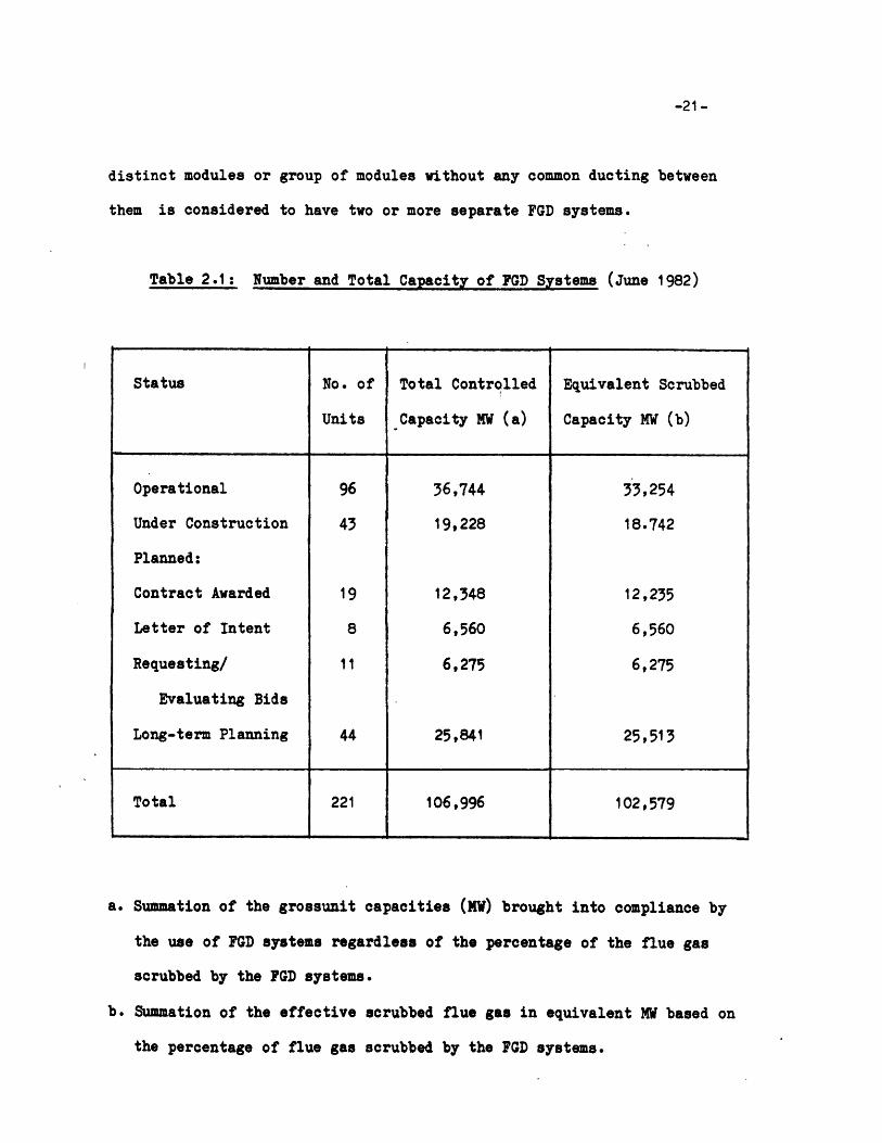
Table 2.1 summarizes the status of flue gas desulfurization (FGD)
systems in the United States at the end of June 1982. (Bruck et. al., 1982)
A system is defined on the basis of inlet gas ducting configuration. A
module or several modules that are commonly ducted to one or more boilers
comprise a single system. Thus, a single FGD module that treats flue gas
from only one boiler is considered a system, just as multiple FGD connected
through a common duct to multiple boilers are considered one system. On
the other hand, a plant that has several boilers ducted to a number of
-21-
distinct modules or group of modules without any common ducting between
them is considered to have two or more separate FGD systems.
Table 2.1: Number and Total Capacity of FGD Systems (June 1982)
a. Summation of the grossunit capacities (MV) brought into compliance by
the use of FGD systems regardless of the percentage of the flue gas
scrubbed by the FGD systems.
b. Summation of the effective scrubbed flue gas in equivalent MW based on
the percentage of flue gas scrubbed by the FGD systems.
Status No. of Total Controlled Equivalent Scrubbed
Units Capacity MW (a) Capacity MW (b)
Operational 96 36,744 33,254
Under Construction 43 19,228 18.742
Planned:
Contract Awarded 19 12,348 12,235
Letter of Intent 8 6,560 6,560
Requesting/ 11 6,275 6,275
Evaluating Bids
Long-term Planning 44 25,841 25,513
Total 221 106,996 102,579
I a I llwil lili hlilllwlli i i id illllim l II NI III I I ,I a III IIIIiIIWII
-22-
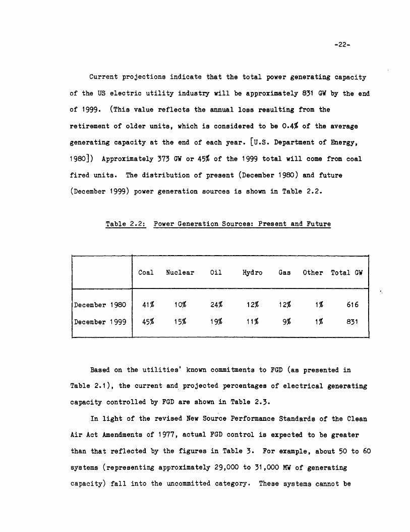
Current projections indicate that the total power generating capacity
of the US electric utility industry will be approximately 831 GW by the end
of 1999. (This value reflects the annual loss resulting from the
retirement of older units, which is considered to be 0.4% of the average
generating capacity at the end of each year. [U.S. Department of Energy,
1980]) Approximately 373 GW or 45% of the 1999 total will come from coal
fired units. The distribution of present (December 1980) and future
(December 1999) power generation sources is shown in Table 2.2.
Table 2.2: Power Generation Sources: Present and Future
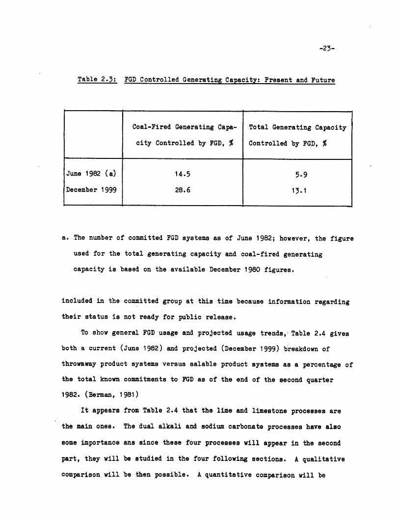
Based on the utilities' known commitments to FGD (as presented in
Table 2.1), the current and projected percentages of electrical generating
capacity controlled by FGD are shown in Table 2.3.
In light of the revised New Source Performance Standards of the Clean
Air Act Amendments of 1977, actual FGD control is expected to be greater
than that reflected by the figures in Table 3. For example, about 50 to 60
systems (representing approximately 29,000 to 31,000 1W of generating
capacity) fall into the uncommitted category. These systems cannot be
Coal Nuclear Oil Hydro Gas Other Total GW
December 1980 41% 10% 24% 12% 12% 1% 616
December 1999 45% 15% 19% 11% 9% 1% 831
MIMINIUMY I
-23-
Table 2.3: FGD Controlled Generating Capacity: Present and Future
a. The number of committed FGD systems as of June 1982; however, the figure
used for the total generating capacity and coal-fired generating
capacity is based on the available December 1980 figures.
included in the committed group at this time because information regarding
their status is not ready for public release.
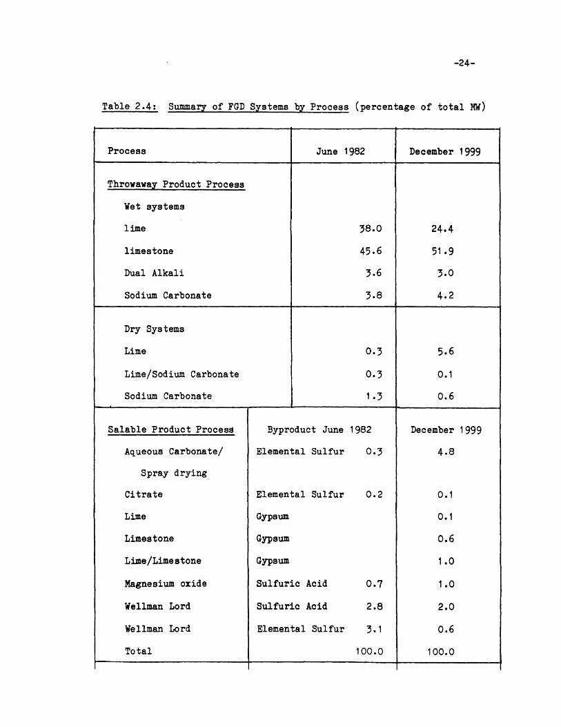
To show general FGD usage and projected usage trends, Table 2.4 gives
both a current (June 1982) and projected (December 1999) breakdown of
throwaway product systems versus salable product systems as a percentage of
the total known commitments to FGD as of the end of the second quarter
1982. (Berman, 1981)
It appears from Table 2.4 that the lime and limestone processes are
the main ones. The dual alkali and sodium carbonate processes have also
some importance ans since these four processes will appear in the second
part, they will be studied in the four following sections. A qualitative
comparison will be then possible. A quantitative comparison will be
Coal-Fired Generating Capa- Total Generating Capacity
city Controlled by FGD, % Controlled by FGD, %
June 1982 (a) 14.5 5.9
December 1999 28.6 13.1
,Eh kiW iiYm
-24-
Table 2.4: Summary of FGD Systems by Process (percentage of total MW)
Process June 1982 December 1999
Throwaway Product Process
Wet systems
lime 38.0 24.4
limestone 45.6 51.9
Dual Alkali 3.6 3.0
Sodium Carbonate 3.8 4.2
Dry Systems
Lime 0.3 5.6
Lime/Sodium Carbonate 0.3 0.1
Sodium Carbonate 1.3 0.6
Salable Product Process Byproduct June 1982 December 1999
Aqueous Carbonate/ Elemental Sulfur 0.3 4.8
Spray drying
Citrate Elemental Sulfur 0.2 0.1
Lime Gypsum 0.1
Limestone Gypsum 0.6
Lime/Limestone Gypsum 1.0
Magnesium oxide Sulfuric Acid 0.7 1.0
Wellman Lord Sulfuric Acid 2.8 2.0
Wellman Lord Elemental Sulfur 3.1 0.6
Total 100.0 100.0

-A N1Y111H1i0
-25-
later detailed in part two.
2.3 Limestone Scrubbing
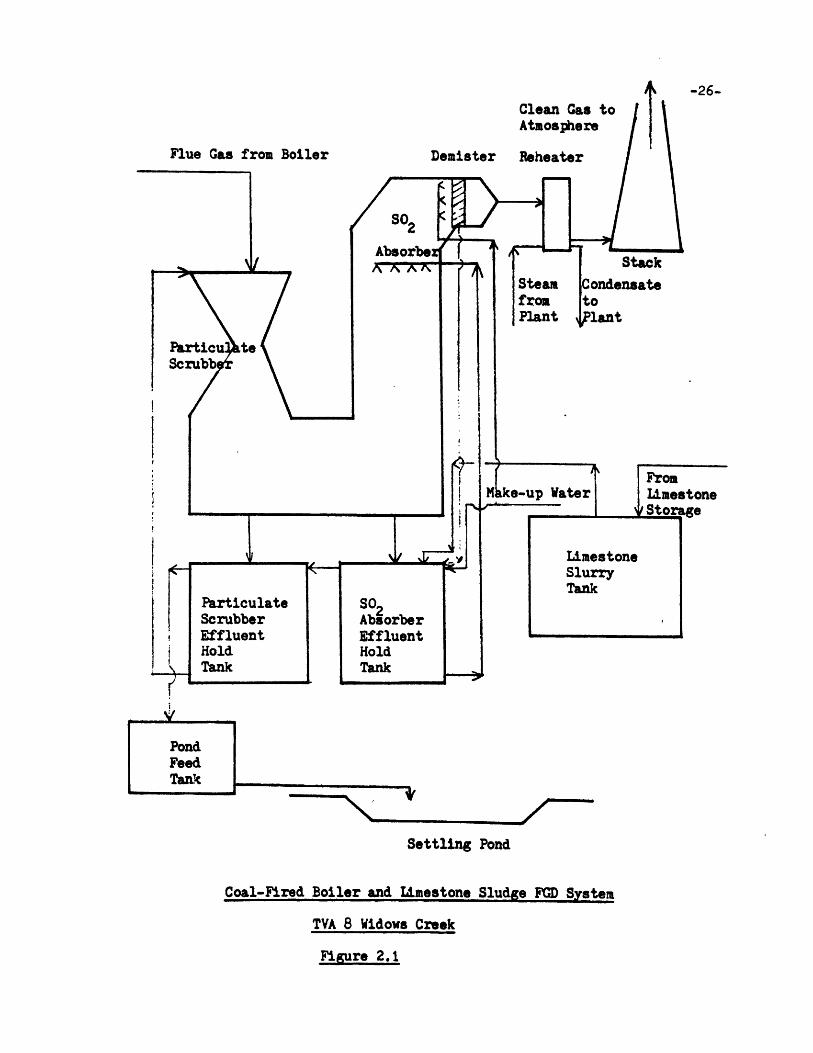
2.3.1 Process Description (Princiotta et. al., 1979)
The principles of all limestone scrubb.ng systems are essentially the
same. When the limestone-water slurry comes in contact with flue gas
containing S02, the SQ2 is absorbed into the slurry and reacts with the
limestone to form an insoluble sludge. The by-products include gypsum
(CaSO4 , 2H2 0) and calcium sulfite hemihydrate (CaSO3 , 1/2 H0). These
sludge by products are generally disposed of in a pond. Figure 2.1 is an
example of a flow diagram of a 500 MW coal-fired boiler with a
limestone/sludge FGD system.
2.3.2 Process Chemistry
The overall reactions that take place in the absorber are:
SO + CaC03 --- > CaSO + CO2 (1)
SO3 + CaC 3 -> CaSQ + C002 (2)
Many intermediate steps also take place, however. The calcium ion is
formed during slurry preparation:
CaCO3 + 20 -- > Ca++ + HC0 + OH- (3)
The S30 anion forms at the flue gas-slurry interface in the absorber.
so2 + H2 0 -- > 12 S0 -- > S03-- + 2H+ (4)
Flue Gas from Boiler
Settling Pond
Coal-Fired Boiler and Limestone Sludge FCD System
TVA 8 Widows Creek
Figure 2.1
Demister Reheater
-IMI
-27-
The sulfite ion (SO--) then combines with the cacium ion (Ca++) to form
the precipitate calcium sulfite hemihydrate:
Ca+ + + Sq-- + 1/2 H20 -- > CaSO3 * 1/2 H20 (5)
Gypsum, an additional precipitate, is formed as follows:
S% -- + 1/2 02 -- > S04-- (6)
Ca++ + S0 -- + 2H20 -- > CaSQ. 2H20 (7)
As reactions 6 and 7 proceed, the calcium cation is depleted from
solution and additional CaC03 dissolves to react with the sulfite ion. In
a limestone sludge system, by-products occur from both reactions 6 and 7.
According to the molecular weights of limestone and SO2 the
theoretical requirement is 1 mol of limestone per mole of S02 removed. If
a 20% excess stoichiometric amount and 95% purity of limestone are assumed,
actual limestone required is 1.97 kg/kg of SO2.
Dry sludge generated in the limestone process consists of calcium
sulfite hemihydrate, carbonates, fly ash, and gypsum. Unused limestone and
limestone impurities also combine with the sludge. The exact proportions
of calcium sulfite hemihydrate and gypsum depend on system design; but if
equal proportions are assumed, the sludge generated is 2.76 kg/kg of SO2.
When a venturi scrubber removes particulate matter, the particulates thus
removed are also combined with the sludge. The final sludge to be disposed
contains at least 20% water.
For instance, the projected mass flow rates of wastes for a 500 MW
power plant assumed to have a 30 year lifetime of 117,500 operating hours
and to operate 6,000 hours in the first year are shown below:
(The fuel is a 3.5% sulfur, 16% ash, 5830 kcal/kg high heat rate bituminous
coal.)
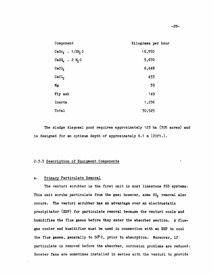
Component
CaSo 3 . 1/2H2 0
CaSOQ . 2 H20
CaC03
CaC12
Fly ash
Inerts
Total
Kilograms per
16,550
5,670
6,448
433
149
1,236
30,525
The sludge disposal pond requires approximately 123 ha (305 acres) and
is designed for an optimum depth of approximately 6.1 m (20ft.).
2.3.3 Description of Equipment Components
a. Primary Particulate Removal
The venturi scrubber is the first unit in most limestone FGD systems.
This unit scrubs particulate from the gas; however, some SO2 removal also
occurs. The venturi scrubber has an advantage over an electrostatic
precipitator (ESP) for particulate removal because the venturi cools and
humidifies the flue gases before they enter the absorber section. A flue-
gas cooler and humidifier must be used in connection with an ESP to cool
the flue gases, generally to 5C C, prior to absorption. Moreover, if
particulate is removed before the absorber, corrosion problems are reduced.
Booster fans are sometimes installed in series with the venturi to provide
-28-
hour
-29-
the power necessary to force the gas through the scrubber system.
b. SO. Absorber
The absorber is the primary S0 2 removal unit in the system. Each of
the many available designs employs a different method to contact the flue
gas with the slurry. The most common unit designs include fixed packing,
mobile-bed packing (hollow or solid spheres), and horizontal or vertical
spray towers. Although each unit performs differently, identical
parameters have the same general effect on performance. Because of its
simplicity, however, the spray tower is gaining popularity.
The scrubber must be constructed of materials that resist corrosion,
erosion and scaling. Scrubber bodies are fabricated of stainless steel or
mild steel lined with an acid resistant coating such as fiber glass
reinforced polyester (FRP), rubber or glass flake. Scrubber internals are
made of a variety of materials such as stainless steel, which has a
tendancy to pit; high nickel alloys, which are expensive; or FRP, which is
fragile. No one material seems to stand above the others.
The size and number of modules in a scrubber system are directly
related to boiler size, turndown (reduction in boiler output) requirements,
system availability, and gas liquid distribution. Boiler system loads
fluctuate, and the srubber system must change to maintain optimum scrubber
performance. One method of adjusting to turndown is to shut down scrubber
modules as the load decreases. The more modules in the system, the
smoother the transition. Scrubber modules not being used can be scheduled
for cleaning and maintenance during periods of low system load, thereby
reducing overall scrubber downtime. The use of multiple modules also has
IIImilmII II 1101IT10- -
-30-
the advantage of permitting the modules to be smaller. Smaller cross
sectional areas in the scrubber module promote uniform gas liquid
distribution and improve efficiency. Scrubber module sizes range from
about 25 to 200 MW.
c. Demister
A demister is necessary to remove entrained droplets from the scrubber
outlet gas to reduce downstream equipment corrosion and scaling and to
reduce reheat requirements. Most of the droplets are large enough to be
removed with a simple change in flue gas direction; this is provided by
baffles. Two banks of demisters are usually sufficient, but more can be
added for additional demisting capability. Demisters are also installed to
reduce this tendency, and materials of construction must be carefully
selected.
d. Reheater
Reheating of stack gas is generally necessary to increase the kinetics
of the reactions described in Section 2.3.2 and to reduce downstream
corrosion. Thus, reheat not only helps meet ambient air standards, it also
protects downstream equipment and prevent formation of acid mist.
Reheating can be accomplished by installing a gas or low sulfur oil burner
that exhausts directly into the stack, or by-passing some hot flue gas
around the FGD system directly into the stack. (increasing emissions of
S02 ) In-line heat exchangers are the most popular because of their low
initial capital cost, but they tend to corrode and scale. Soot blowers,
better demisters, and better materials of construction reduce these
___________________________________Imuri iIIfIIIIUp
-31-
problems.
e. Slurry Makeup
Limestone can be received in a crushed and milled state or can be
crushed and milled on site. In the latter case, the limestone is ground
(wet or dry) in a ball mill to a size not larger than 200-mesh and often
finer than 325-mesh. Finer grinding reduces the amount of limestone that
remains unreacted and would otherwise be disposed of in the sludge. Water
is added until the solids content reaches 15 to 25%. The slurry is then
sent to a feed tank and to an absorber holding tank where it is mixed with
aborber effluent. The slurry from the absorber holding tank is pumped to
the absorber, where it reacts with Sq2 in the flue gas and is then returned
to the holding tank. Slurry from the absorber holding tank is pumped to
the venturi holding tank and from there to the venturi to scrub out fly
ash. The slurry containing the fly ash returns to the venturi holding
tank, from which it is pumped to the sludge disposal area for final
treatment.
f. Sludge Disposal
Sludge disposal can require 200,000 m2 at a small plant and as much as
4,000,000 m2 at a large plant. Disposal practices are very site specific.
A power plant in an arid location might pump the sludge into an unlined
pond, allowing the water to evaporate or seep into the ground. In an area
where surface runoff or leaching could be a problem, the sludge sometimes
is dewatered before being pumped into a lined pond. The water is returned
to the system or purged after treatment to reduce chloride ions in the slurry.
I IJIMMMM
-32-
2.3.4 Advantages and Disadvantages
The process is well developed chemically, but mechanical problems are
still encountered in certain facilities as described in sections 4 and 5.
These problems include: fan vibration; pump and pipe erosion; scale
buildup in the scrubber, demister and reheat sections; potential pollution
in openwater systems; and corrosion and erosion.
The system operates well on large boilers. On small systems with low
operating factors, labor and capital charges can be a limiting factor.
Strict solid waste and water regulations either in force or imminent could
necessitate more careful consideration of sludge disposal approaches. It
may be necessary to incorporate an oxidation step to produce acceptable £
materials for landfill disposal. The advantages of the limestone/sludge
systems can be summarized as follows:
(1) The basic process is fairly simple and has few process steps.
(2) The reserves of limestone are fairly abundant.
(3) S02 removal efficiencies can be as high as 95%.
(4) The two-stage treatment of flue gases permits removal of S02 and
particulates.
(5) Many years of operating experience have led to a greater understanding
of the basic principles of this process.
(6) Fly ash does not adversely affect the system.
The disadvantages of the limestone/sludge systems are as follows:
(1) Large quantities of waste must be disposed of in an acceptable manner.
(2) If not designed carefully or operated attentively, limestone systems
-33-
have a tendency toward chemical scaling, plugging, and erosion which
can frequently halt its operation.
(3) The scrubber requires high liquid-to-gas (L/G) ratios necessating
large pumps with attendant electrical requirements.
(4) The sludge may have poor settling properties when it has high sulfite
content. Forced oxidation or soluble Mg in the slurry have been shown
to lower sulfite content.
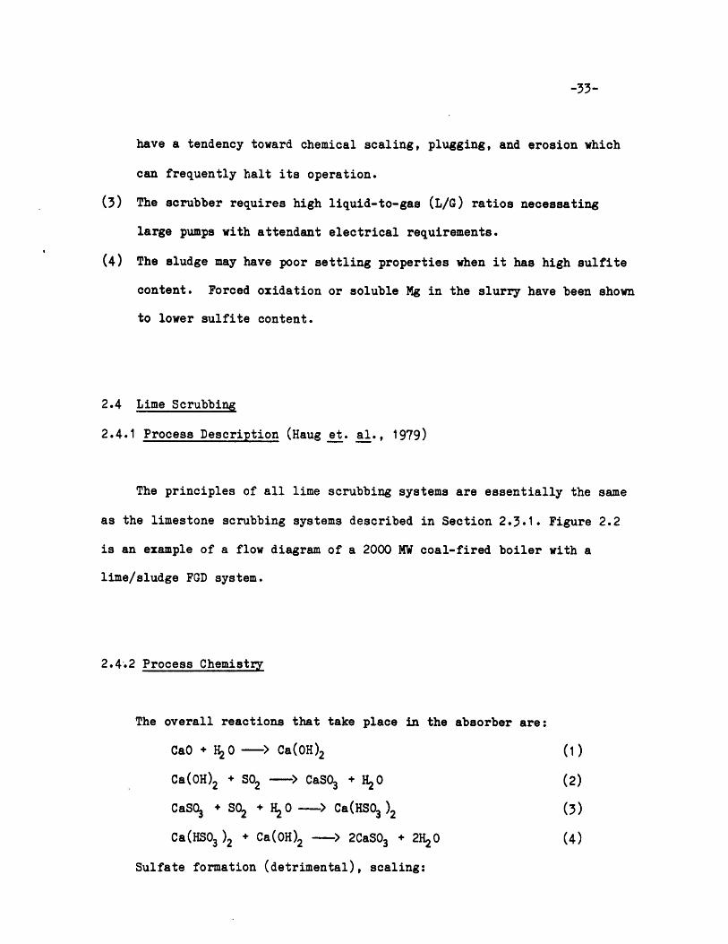
2.4 Lime Scrubbing
2.4.1 Process Description (Haug et. al., 1979)
The principles of all lime scrubbing systems are essentially the same
as the limestone scrubbing systems described in Section 2.3.1. Figure 2.2
is an example of a flow diagram of a 2000 MW coal-fired boiler with a
lime/sludge FGD system.
2.4.2 Process Chemistry
The overall reactions that take place in the absorber are:
CaO + 1 0 -- > Ca(OH)2 (1)
Ca(OH)2 + S02 -- > CaSO3 + H2 0 (2)
CaSO3 + 02 + H ---> Ca(HSO3 )2 (3)
Ca(HSO3 )2 + Ca(OH)2 -- > 2CaSO3 + 2H20 (4)
Sulfate formation (detrimental), scaling:
i __^___ 11111 W1
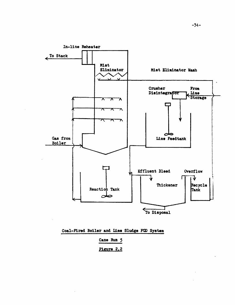
In-line Reheater
Mist Eliminator Wash
Coal-Fired Boiler and Line Sludge FGD System
Cane Run 5
Figure 2,2
-34-
__i;_;~l_ ___ ~__iij _1^_1____ _ _~ I__=__;_;__ ~_V_~ __~ ~_ ~
-35-
2CaSO3 + 02 -- > 2CaSQ, (5)
Scrubbing liquor is a slurried mixture of calcium hydroxide and
calcium sulfite in water. The pH of slurry entering the scrubber is 8 to
10. Low pH can cause gypsum scaling whereas high pH can cause formation of
carbonates. The presence of MgO in the lime allows a subsaturated mode of
operation and improves the Sq removal efficiency.
The reaction with S02 in the flue gas takes place in the liquid phase.
The dissolution of calcium sulfite is the rate controlling step for S02
absorption. In other cases the mass transfer through the interface between
gas and liquid is the rate controlling step.
2.4.3 Description of Equipment Components
The equipment components are similar to those described for the
limestone scrubbing process.
2.4.4 Advantages and Disadvantages
Generally inexpensive lime can be provided to the FGD plants and, as
far as available, carbide sludge from chemical industry or alkaline fly ash
can be utilized as scrubbing agent. The lime scrubbing technology is well
developed. Current R&D efforts aim at the following chemical, mechanical
and design areas:
- Precipitation of calcium sulfate (gypsum) may cause scaling, which is
_ -- ~ ^- 1 111mmmm 11mmun1m 1m1m mm......1
-36-
particularly unwanted in mist eliminators.
- Dissolved salts in the scrubbing agent and chloride built-up in the
recycle water can cause corrosion, which is possibly aggravated by the
erosive nature of the slurry.
- Pumps, fans and agitators allow mechanical improvements as to their use
in this technology.
- Interrelated mechanical and chemical factors may influence the lifetime
of expansion joints and piping.
- Finally the optimization of the design parameters like gas flow and
slurry distribution, liqid-to-gas ratio, control instrumentation and
accessibility for maintenance has to be mentioned.
The advantages of the lime scrubbing system are similar to those
listed for the limestone scrubbing process.
The disadvantages are also similar to those listed for the limestone
scrubbing process. In addition, although fly ash does not adversely affect
the process in general it can adversely affect the process by
intensification of mechanical wear and erosion in the washing cycle and by
increased load of the thickener.
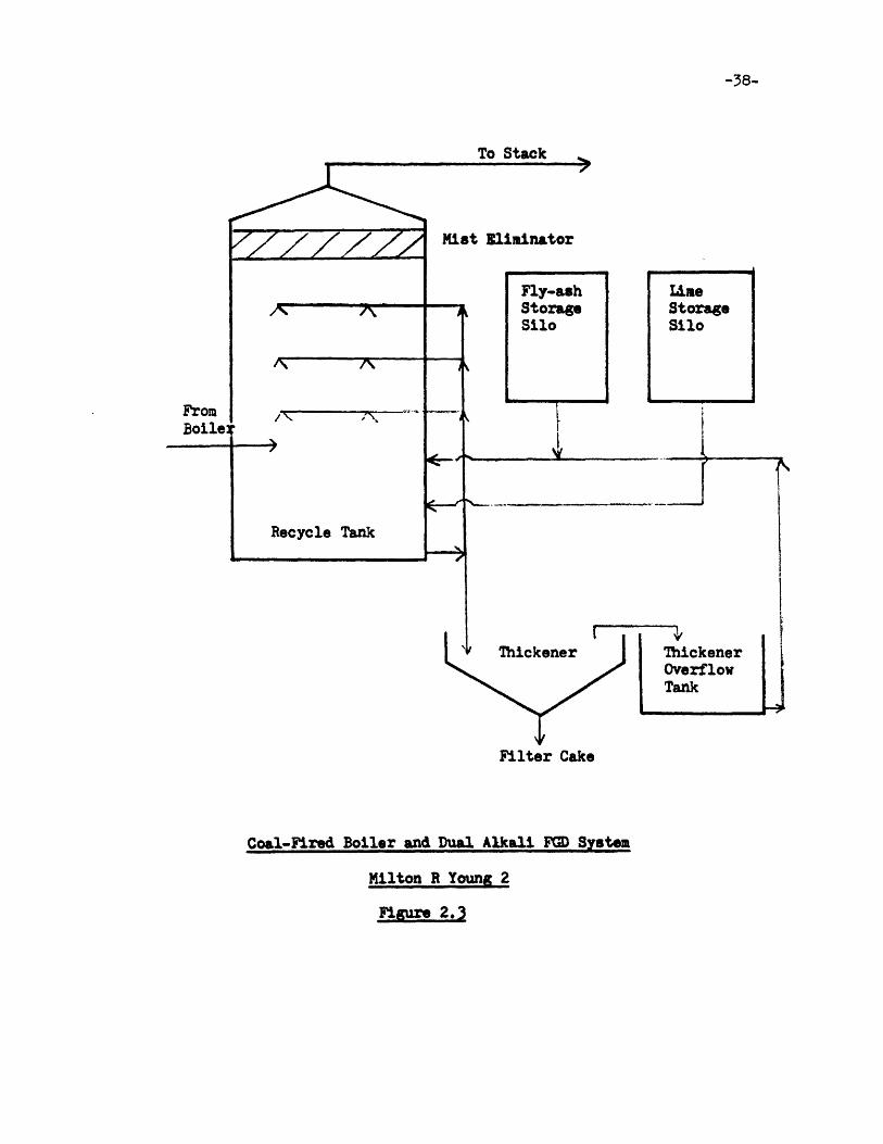
2.5 Dual Alkali Scrubbing
2.5.1 Process Description (Kaplan, 1979)
As in the limestone slurry system, dual-alkali processes dispose of
removed S02 as throwaway calcium sludge. Unlike limestone, however,
absorption of S02 and production of disposable waste are separated; the

___III M min In IIN mIIu.
-37-
addition of limestone or lime occuring outside the scrubber loop. The
scrubbing step uses an aqueous solution of soluble alkali. The absorption
reaction depends on gas/liquid chemical equilibrium and mass transfer rates
of sulfur oxides (SO ) from flue gas to scrubbing liquid instead of
limestone dissolution, the limiting factor in limestone scrubbing.
Therefore, SOx absorption efficiency in a double-alkali system is
potentially higher than in a limestone system with the same physical
dimensions and liquid-to-gas (L/G) flow rates. Scaling and plugging in the
absorption area are reduced because calcium slurry is confined to the
regeneration and disposal loop and soluble calcium is minimized in the
scrubber liquor. Figure 2.3 is an example of a flow diagram of a 125 MW
coal-fired boiler with a dual-alkali scrubbing FGD system.
2.5.2 Process Chemistry
Technically, the use of any combination of alkaline compounds, organic
or inorganic, for SQ2 removal and disposal can be classified as a dual-
alkali process. The process described in this section is a sodium sulfite
absorbent-lime reactant system.
Sodium sulfite in solution absorbs S02 in the scrubbing step
represented by equation (1):
S0" + so2 + o --- > 2HSO3 (1)
Sodium hydroxide formed in the regeneration step and sodium carbonate added
as solution makeup react with S02 as shown below. The absorption reactions
actually involve reaction of SQ2 with an aqueous base such as sulfite,
gi ~ i IIIIIIlI I4
-38-
To Stack
Mist Eliminator
ii j
Fly-ashStorageSilo
I
IAmeStorageSilo
I
Thickener 'ThickenerOverflowTank
Filter Cake
Coal-Fired Boiler and Dual Alkali FGD System
Milton R Young 2
Figure 2.3
FromBoiler
Recycle Tank
I I I 1 III I~--,,r----l; T----~C--~I~C-~- ~_i_~_--ih-- ----~- ---~---J ----- -; ------- --~ ~ '
I~ ___~ i
-39-
hydroxide, or carbonate rather than sodium ion which is present only to
maintain electrical neutrality.
20H- + s 2 -- -- + 0 (2)
o-- + S02 -> So-- + Co2 (3)
The use of lime for regeneration allows the system to be operated over
a wider pH range which in turn included the complete range of active alkali
hydroxide/sulfite /bisulfite. Limestone regeneration operates only in the
sulfite/bisulfite range.
Ca(OH)2 + 2HSO- --- S03 - + CaSO . 1/2 H20 + 3/2 H20 (4)
Ca(OH)2 + S03" + 1/2 H20 -- > 20H- + CaS03 . 1/2 H20 (5)
Ca(OH)2 + S" --- > 20H- +Casq (6)
Ca(OH)2 + So04 + 2H20 -- > 20H- + CaSk . 2H20 (7)
Total oxididizable sulfur (TOS) is the total concentration of sulfite
and bisulfite in solution. Oxidation of TOS to sulfate may occur in any
part of the system and is affected by composition of the scrubbing liquor,
oxygen content of the flue gas, impurities in the lime, and design of the
equipment.
s03-- + 1/2 02 -- > Sc (8)
HS0- + 1/2 02 --> So"4 + H+ (9)
The sum of concentrations of NaOH, Na2CO3 , NaHCO3 , Na2S03 and NaHS03
in the scrubbing solution is termed active alkali. The active alkali
concentration in a system can be dilute or concentrated; a concentrated
mode (active concentration of sodium greater than 0.15 M) was chosen for
this discussion. In this mode high sulfite levels prevent the
precipitation of calcium sulfate (CaSO4 ) as gypsum (CaSO4 . 2H20), equation
7. However, CaSQ, is precipitated along with calcium sulfite (CaSO3 * 1/2
~ 1 ~ I 11N
-40-
H2 0) as shown in equations 4-6. In this way the system can keep up with
sulfite oxidation at the rate of 25 to 30% of the S02 absorbed without
becoming saturated with CaSQ,. Usually, soluble calcium levels are less
than 100 ppm in the regenerated liquor of a concentrated mode dual-alkali
process.
2.5.3 Description of Equipment Components
The dual-alkali process has been divided into the following operating
areas:
- Materials Handling. This area includes facilities for receiving pebble
lime from an across-the-fence limestone calcination plant, lime storage
silo, and in-process storage for supply to the slakers. Soda ash storage
is also provided.
- Feed Preparation. Included in this area are two parallel slaking systems
and the facilities for dissolving makeup soda ash in water before feeding
to the absorption system.
- Gas Handling. Fan location and duct configuration are the same as in the
limestone scrubbing process.
- S02 Absorption Four tray tower absorbers with presaturators,
recirculation tanks, and pumps are included.
- Stack Gas Reheat. Equipment in this area includes indirect steam
reheaters and soot blowers for the coal variations.
- Reaction. Reaction tanks with agitators and pumps are provided in this
area.
-41-
- Solids Separation. Separation of calcium salts is accomplished by
thickener and filters.
- Solids Disposal. Filter cake is reslurried in this area and purged to
the disposal pond. A pond return pump is included.
2.5.4 Advantages and Disadvantages
System reliability can be adversely affected by two classes of
problems: mechanical and chemical.
Mechanical problems include malfunction of instrumentation and
mechanical and electrical equipment such as pumps, filters, centrifuges,
and valves. These problems in a commercial FGD system can be minimized by
careful selection of materials of construction and equipment and by
providing spares for equipment items such as pumps and motors which are
expected to be in continuous operation.
Chemical problems which may be associated with a dual-alkali system
include scaling, production of poor-settling solid waste product, excessive
sulfate buildup, water balance, and buildup of nonsulfur solubles which
enter the system as impurities in the coal or lime.
One of the primary reasons for development of dual-alkali processess
was to circumvent the scaling problems associated with lime/limestone wet
scrubbing systems. Since scrubbing in dual-akali systems employs a clear
solution rather than a slurry, there is a tendency to ignore potential
scaling problems. However testing experience has indicated that scaling
can occur and be particularly troublesome since the flue gas path through
-42-
the scrubber can shut down the boiler/scrubber system and lower reliability.
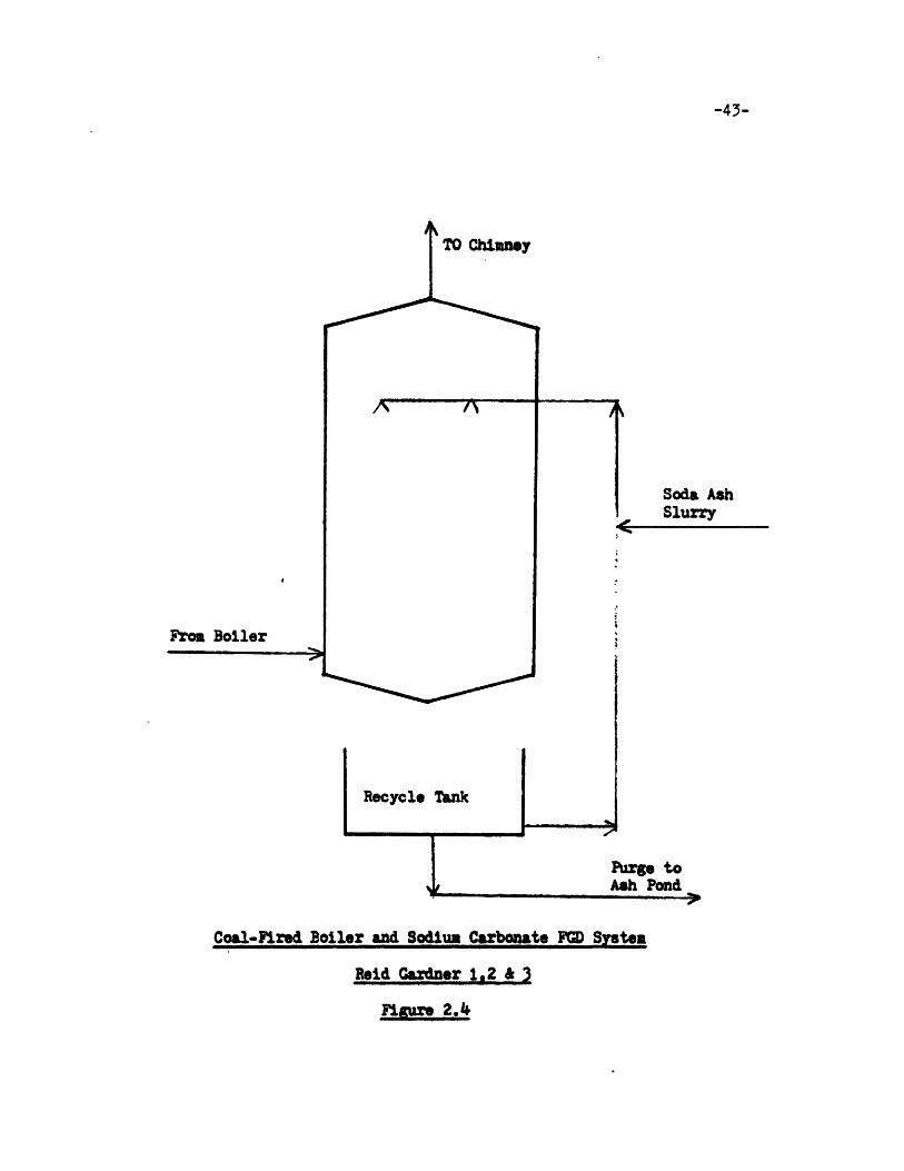
2.6 Sodium Carbonate Scrubbing
2.6.1 Process Description (Slack et. al., 1975)
The sodium carbonate method is shown in figure 2.4. Addition of
Na2 C03 to the thickener precipitates enough calcium to keep the calcium
content of the liquor to the scrubber well on the safe side of saturation
(about 100 ppm below saturation). It is expected that the Na2C03 makeup
requirement will be at least very high because of losses in the filter
cake.
2.6.2 Process Chemistry
In the absorption section, absorption of S02 in sodium sulfite
solution produces a bisulfite scrubber effluent solution according to the
overall reaction:
Na2 S O3 + S02 + H20 -- > 2NaHSO3 (1)
The sodium carbonate used as sodium makeup to the system forms sodium
sulfite in the scrubber:
Na2CO + SO2 -> Na 2 S03 + Co2 (2)
The absorber feed solution will also contain sodium sulfate in solution and
may contain some sodium bisulfite if neutralization is not completed in the
regneration section. The sulfate is formed in the scrubber by reaction of
Ill__ _ _ _ _ _l i II
-43-
TO Chimney
From Boiler
Recycle Tank
SSoda AshSlurry
Purge toAsh Pond
Coal-Fired Boiler and Sodium Carbonate FGD System
Reid Cardner 1.2 & 3
F lgur 2,4
-44-
sulfite with oxigen in the flue gas:
2Na 2 S03 + 02 -- > 2Na 2 SQ~ (3)
The rate of oxidation is a function of the absorber design, oxigen
concentration in the flue gas, flue gas temperature, and the nature and
concentration of the species in the scrubbing solution. As an example, for
flue gas containing about 4 to 5% 02 and 2,500 ppm S02, approximately 10%
of the SC removed from the flue gas will normally be oxidized to sulfate.
The neutralization goes to completion with lime:
Na2 SO3 + Ca(0H) 2 -- > 2NaOH + CaSO3 (4)
The usual form of calcium sulfite produced is the Hemihydrate, CaSO3 . 1/2
H2 0. Some sulfate is also precipitated, the amount depending on the
sulfite and sulfate concentration and on pH.
2.6.3 Description of Equipment Components
The equipment components are similar to those decribed for the
limestone scrubbing process.
2.6.4 Advantages and Disadvantages
The main drawback is that the sulfate formed incidentally by oxidation
in the scrubber and in other parts of the system is more difficult to
regenerate than when other absorbents are used. Much of the research in
the area is concerned with this problem.
-45-
3 COST ANALYSIS OF PROVEN PGD
3.1 Introduction
The cost of Flue Gas Desulfurization (FGD) systems is an area of
intense interest and substantial controversy. Few realistic cost figures
have been established.
In section 2, the main FGD processes were described by looking at
different technical advantages and disadvantages. However, these
differences were not translated into actual dollar figures.
The following economic analysis considers the FGD systems whose
commercial start-up occurred before the end of 1977. At least four years
(78,79,80,81) of data about these devices are available. Devices that have
been in use this long are referred to as proven FGD. The FGD systems are
not pilots and are installed on relatively large scale plants, units of at
least 50 MW. The processes used by these systems are the four processes
described in section 2.
Section 3.2 contains an overview of the proposed methodology with
emphasis on the data collection, the cost elements description and the cost
adjustment procedure.
In section 3.3, the results obtained by applying this methodology are
shown. The four main processes used by systems installed on either old or
new plants are compared. Their capital and annual costs and their energy
consumptions are analyzed. Then the impact of these costs on the consumer
and the producer is studied. Finally, in the conclusion, a comparison is
made with another FGD cost analysis.
_ IIIIYI YI l ll IIIYIIIIII lllll III1I
-46-
3.2 Description of the methodology
3.1.1 Collection of the data
The reported figures are acquired from various sources. (The most
reliable information was obtained from a previous cost study initiated by
PEDCo Environmental in March 1978. (Devitt et. al., 1980) In this first
study each utility with at least one operational FGD system was given a
cost form containing all available cost information then in the PEDCo
files.
The utility was asked to verify the data and fill in any missing
information. The PEDCo Environmental staff made a follow-up visit to
complete and verify the data collected.
Some costs were also taken from FGD cost survey questionnaires
developed by Edison Electric Institute (EEI). The EEI forms contain useful
capital cost information, however, in some cases the costs were projections
rather than actual dollar expenditures.
In addition to the sources just mentioned some 1978 and 1979 annual
costs were made available by a few utilities via written transmittals and
telephone communications.
3.2.2 Description of Cost Elements
Capital costs, expressed in $/kW, consist of direct costs, indirect
costs and other capital costs. Direct costs include the cost of the
equipment (scrubber, pump, fan,...), the cost of installation (piping,
instrumentation) and the site development (construction of access roads,
-47-
truck facilities,...). Indirect costs include interest during
construction, contractor's fees and expenses, engineering, legal expenses,
taxes, insurance, allowance for start-up and shakedown and spares. Other
capital costs include contingency costs (malfunctions, equipment
alterations, unforeseen sources), land for waste disposal and working
capital (amount of money invested in raw materials and supplies in stock).
Annual costs, expressed in mills/kWh, consist of direct costs, fixed
costs and overhead costs. Direct costs include the cost of raw materials
(lime, limestone,...) utilities (water, electricity,...), operating labor
and supervision and maintenance and repairs. Fixed costs include those of
depreciation, interim replacement, insurance, taxes and interest on
borrowed capital. Overhead costs include those of plant and payroll
expenses. Although they are not charged directly to a particular part of a
project like FGD, they are allocated to it.
3.2.3 Cost Adjustment Procedure
In order to compare the FGD systems on a common basis, the following
cost adjustments were made:
1. All capital costs are adjusted to 1981 dollars, using' the
escalation factors shown in Table 3.1. Actual costs were reported by
utilities in dollar values since the start up date. The total figure is
broken down into dollars per year and each year total is escalated to 1981
dollars and totaled again.
2. Particulate control costs are deducted. Since the purpose of the
IIYmmm mmmmNNmmanmN 1um In 111 1H , I. II l IIlI llM
-48-
study is to estimate the incremental cost for sulfur dioxide control,
particulate control costs are deducted using either data contained in the
costs breakdowns or as a percentage of the total direct cost, capital and
annual.
3. All non-labor annual costs are adjusted to a common 65% capacity
factor, assuming a continuous operation of 8#760 hours.
4. Sludge disposal costs are adjusted to reflect the costs of sulfur
dioxide waste disposal only (i.e., excluding fly ash disposal except where
usable as a sludge stabilizing agent) and to provide for disposal over the
anticipated lifetime of the FGD system. This latter correction is
necessary since several utilities reported costs for sludge disposal
capacity that would last only a fraction of the FGD system life. The
adjustments are based on a land cost of $2000/acre with a sludge depth of
50 ft in a clay lined pond (clay is assumed to be available at the site).
5. A 30 year life, value recognized by the National Power Survey of
the Federal Power Commission, is assumed for all new systems that were
installed for the life of the unit.
A 20 year life is assumed for retrofit systems that were installed for
the life of the unit.
3.3 Results and Interpretation
3.3.1 Introduction
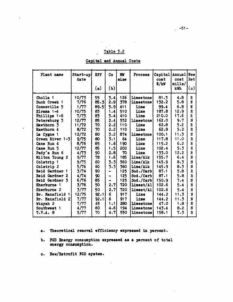
The detailed results are shown in Table 3.2. Twenty-six plants
correspond to the definition given in the introduction. The four main

-49-
Table 3.1
Escalation Factors
Year (a) Capital Utilities Chemicals Operation & Cons
Investment (c) (d) Maintenance Labor
(b) Labor (e) (f)
1970 0.537 0.238 0.550 0.540 0.542
1971 0.576 0.277 0.584 0.583 0.613
1972 0.600 0.321 0.603 0.630 0.669
1973 0.624 0.372 0.624 0.681 0.704
1974 0.738 0.496 0.733 0.735 0.768
1975 0.825 0.665 0.819 0.794 0.824
1976 0.875 0.762 0.866 0.857 0.887
1977 0.934 0.873 0.928 0.926 0.937
1978 1.0 1.0 1.0 1.0 1.0
1979 1.09 1.1 1.075 1.08 1.08
1980 1.188 1.21 1.156 1.166 1.166
1981 1.295 1.331 1.242 1.260 1.260
a. cost index is for mid-year (June)
b. reference: Marshall and Swift
c. includes fuel and electricity; reference: Department of Commerce
d. reference: Bureau of Mines
e. reference: Department of Labor
f. reference: Engineering News Record (Construction Labor)
III IIIIIYUIIYY iY YIIIIIIYI- 1" 1,0 1'J111 ,1,1li1 1jh,,,I i di01101 0 01 F -o l
-50-
processes described in Section 2 are represented here. The dual alkali
process is used either with lime or limestone. If the sodium carbonate
process which represents a small portion of FGD systems, is not taken into
account there are just two categories: the lime and the limestone process.
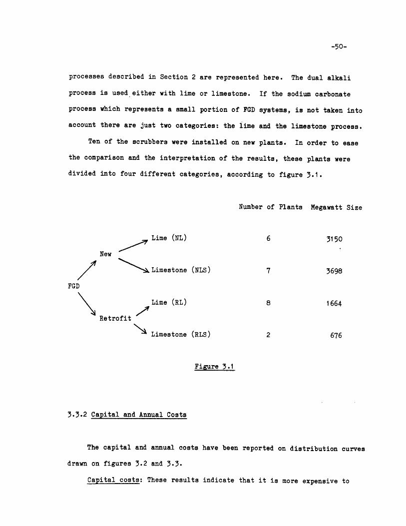
Ten of the scrubbers were installed on new plants. In order to ease
the comparison and the interpretation of the results, these plants were
divided into four different categories, according to figure 3.1.
Number of Plants Megawatt Size
Lime (NL) 6 3150
New
Limestone (NLS) 7 3698
FGD
Lime (RL) 8 1664
Retrofit
Limestone (RLS) 2 676
Figure 3.1
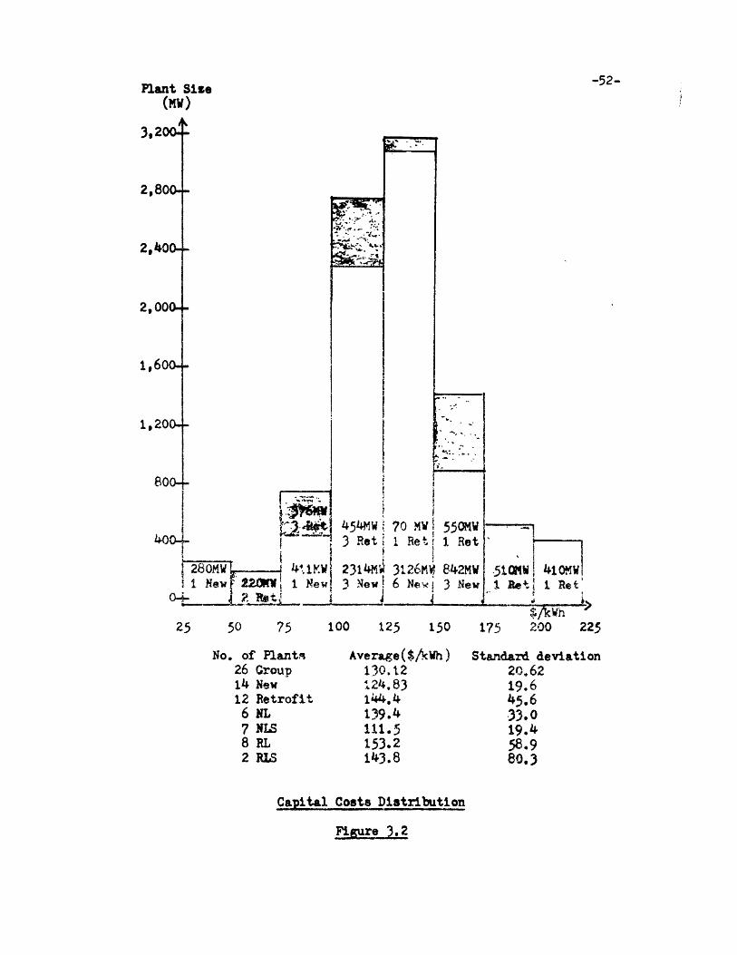
3.3.2 Capital and Annual Costs
The capital and annual costs have been reported on distribution curves
drawn on figures 3.2 and 3.3.
Capital costs: These results indicate that it is more expensive to
-51-
Table 3.2
Capital and Annual Costs
Plant name Start-up Eff Co MW Process Capital Annual Newdate size cost cost Ret
$/kW mills/(a) (b) kWh (c)
Cholla 1 10/73 55 3.4 126 Limestone 81.3 4.8 RDuck Creek 1 7/76 85.3 2.9 378 Limestone 132.2 5.8 NConesville 5 1/77 89.5 3.9 411 Lime 99.4 6.8 NElrama 1-4 10/75 83 1.4 510 Lime 187.8 12.9 RPhillips 1-6 7/73 83 3.4 410 Lime 210.0 17.6 RPetersburg 3 12/77 85 2.4 532 Limestone 162.0 9.7 NHawthorn 3 11/72 70 2.2 110 Lime 62.8 5.2 RHawthorn 4 8/72 70 2.2 110 Lime 62.8 5.2 RLa Cygne 1 12/72 80 3.2 874 Limestone 100.1 11.3 NGreen River 1-3 9/75 80 3.1 64 Lime 117.8 11.0 RCane Run 4 8/76 85 1.6 190 Lime 115.2 6.2 RCane Run 5 12/77 85 1.5 200 Lime 102.4 5.3 RPady's Run 6 4/73 90 2.8 70 Lime 133.0 12.2 RMilton Young 2 9/77 78 1.6 185 Lime/Alk 155.7 6.4 NColstrip 1 9/75 60 3.3 360 Lime/Alk 145.9 8.3 NColstrip 2 5/76 60 3.3 360 Lime/Alk 145.9 8.3 NReid Gardner 1 3/74 90 - 125 Sod./Carb 87.1 5.8 RReid Gardner 2 4/74 90 - 125 Sod./Carb 87.1 5.8 RReid Gardner 3 6/76 85 - 125 Sod./Carb 150.9 7.4 NSherburne 1 3/76 50 2.7 720 Limest/Al 102.6 5.4 NSherburne 2 3/77 50 2.7 720 Limest/Al 102.6 5.4 NBr. Mansfield 1 12/75 92.1 6 917 Lime 144.2 11.3 NBr. Mansfield 2 7/77 92.1 6 917 Lime 144.2 11.3 NWinyah 2 7/77 45 1.1 280 Limestone 47.0 1.8 NSouthwest 1 4/77 80 4.6 194 Limestone 143.4 8.2 NT.V.A. 8 5/77 70 4.7 550 Limestone 158.1 7.3 R
a. Theoretical removal efficiency expressed in percent.
b. PGD Energy consumption expressed as a percent of totalenergy consumption.
c. New/Retrofit FGD system.
Plant Size(MW)
3,200-
2,800--
2,00- -
2,000--
1,6oo.-
1,200- -
800- -
280MW 4 4l.1WI1 New 22KW I Newl
04- 2 Re
454Mw3 Ret
2314M?3 NewiJ
70 MWI Ret
3126M'6 Ne w
550MW1 Ret 1
842MW3 New
4i I Relt' I Re. '
25 50 75 100 125 150 175 200 225
No. of Plant,26 Group14 New12 Retrofit
6 NL7 NLS8 RL2 RLS
Average($/kWh)130.12124.83144.4139.4111.5153.2143.8
Standard deviation20.6219.645.633.019.458.980.3
Capital Costs Distribution
Figure 3.2
-52-
-'---' I----'
-53-
Plant Size(MW)
4,600.-
3,60(H-
3, 20
2,8 -
2,40
2,00
1,60
1,2
8004.
28NMW1 New l not
1410MW7 Rt
2539MV6 New
2.5
1444 New
7.5
134 MW2 Ret
2708MV3 New
510KV 410KVI Rot 1 Ret
Mills/Wh10 12.5 15 17.5
No. of Plants26 Group14 New12 Retrofit
6 NL7 NLS8 RL2 RLS
Average(Mills/kWh) Standard deviation8.7 1.78.4 1.89.6 3.19.7 2.97.3 2.0
11.3 4.56.8 3.6
Annual Costs Distribution
FYiur 3.3
_
-54-
install a FGD system on an already existing plant than to build both a new
scrubber and a new plant.
The numbers given in Table 3.2 indicate that there are 12 FGD retrofit
systems with a total size of 2590 MW and 14 new FGD systems with a total
size of 6973 MW. Therefore the average retrofit unit size is 216 MW
whereas the average new unit size is 498 MW. As stated by the economic
principle of economies of scale, the bigger the size of the unit, the less
the capital cost will be. The following interpretation reinforces the
former one. It is cheaper to design both a new plant and a new scrubber
rather than trying to design a scrubber which will fit an old boiler "as
well as possible"
The standard deviation is lower than average for the new plants, which
means that the capital costs are about the same. On the other hand, the
capital costs for retrofit systems are spread on a wide range, from
$62.80/kW for Hawthorn 3 and 4 to $210.00 for Phillips 1-6.
The results by category show that the limestone process installed on
new plants (NLS) has the lowest capital cost. The other results are not as
meaningful since there is a very high standard deviation which cannot lead
to a general interpretation.
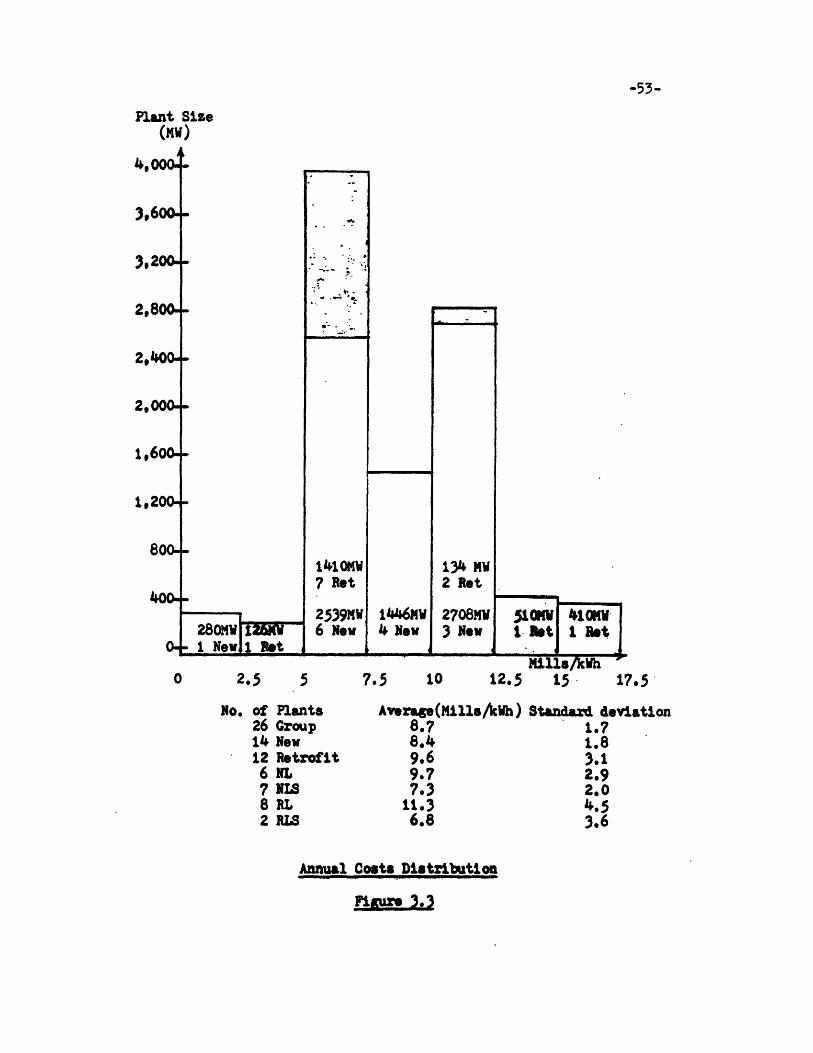
Annual Costs: The annual costs are again higher for retrofit plants
and spread on a wide range from 4.8 mills/kWh for Cholla 1 to 17.6
mills/kWh for Phillips 1-6. The cheapest annual costs are obtained once
again by the NLS cataegory. The RLS category is not considered because
there were only 2 plants and the standard deviation was quite high. A
possible explanation lies in the very cheap price of the limestone which
was in 1980 about $11.60 per ton versus a price of $46.00 per ton for the
-55-
lime. This may also explain the curious shape of the distribution curve
with two peaks: one between 5 and 7.5 mills/kWh, the other between 10 and
12.5 mills/kWh. Most of the lime processes are represented by the second
peak whereas most of the limestone processes are represented by the first
peak.
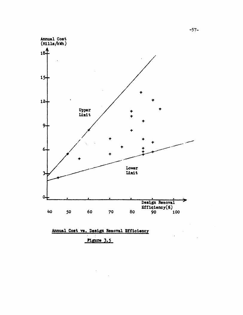
It is interesting to determine the relation between the annual cost
and the design removal efficiency given in Table 3.2. This curve has been
drawn on Figure 3.5. As expected, the greater the efficiency, the more
expensive the annual cost is. The different points are not on a straight
line. However the limits can be drawn. Between the upper limit and the
lower one all the points can be found. The slope of the upper limit is
greater, which means that the greater the efficiency, the larger the range
of the annual cost.
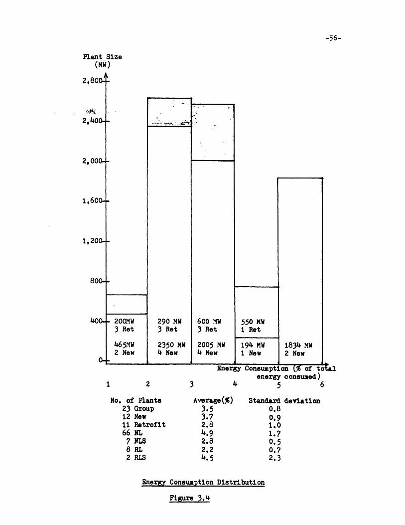
3.3.3 Energy Consumption
The distribution curve of the energy consumption expressed in percent
of the total MW capacity has been drawn in Figure 3.4. The energy
consumption is higher for new (3.7%) than for retrofit FGD systems (2.8%).
The following explanation may be given. If an FGD system is retrofitted to
an existing boiler the new electrical power demand of the FGD equipment
will decrease the boiler net MW rating. Since the boiler was originally
sized and designed to accomodate a certain grid demand, the utility may be
forced to buy make-up power from the grid and/or increase the design
capacity of planned boilers. Therefore the energy consumption for retrofit
T IIMINN =11 Y1Y Y6
-56-
Plant Size(MW)
2,8004
2, 400.
2, 000.
1,600.
1,200-
800-4
400-
0-
- 200MW3 Ret
465MW2 New
290 MW3 Ret
2350 MW4 New
e.
600 MW3 Ret
2005 MW4 New
550 M1 Ret
194 MW1 New
1834 MW2 New
Energy Consumption (% of totalenergy consumed)
2 3 4 5 6
No. of Plants23 Group12 New11 Retrofit66 NL
7 NLS8 RL2 RIS
Average(%)3.53.72.84.92.82.24.5
Standard deviation0.80.91.01.70.50.72.3
Energy Consumption Distribution
Figure 3.4
-57-
Annual Cost(MillsA/kh)
++ ~ 7"
40 50 60 70 80 90 - -o00
Annual Cost vs. Desigu% Removal Efficiency
Figure 3.5
----- unilrul rrlllllri Irlivlirl~
I, ,,I II I II I
systems will be designed as low as possible.
For a new system the problem is not the same. The energy consumption
required by the FGD system will be determined at the same time as the
boiler size so that both work properly. The high price of energy will of
course make it necessary to obtain a low energy consumption but it is not
as imperative as for a retrofit system.
3.3.4 Impact on Consumer/Producer
The average annual cost of the FGD technology is about 9 mills per kWh
(See Figure 3.3). It represents about 15% of the price of a kWh if we
consider an average price of 60 mills for one kWh. This setms to confirm
the claim that scrubbers would add at least $4 a month to the average home
utility bill. (Dumanoski, 1982) The objective of this section is to
determine the distribution of FGD cost between producer and consumer.
The study of electricity rates and more generally of the American
electricity supply is very complicated. American electricity supply is
decentralized into a patchwork of geographically separate operations. This
is very well described by Wilcox and Shepherd. (Wilcox et. al., 1975)
To explore the behavior of regulated firms, a variant of the standard
Averch-Johnson model (Anderson et. al., 1979) can be used. The standard
Averch-Johnson model shows that a monopoly constrained in its decisions by
a regulatory agency to earn a "fair rental" greater than the rental it
would earn in a perfectly competitive market will use relatively more
capital and less labor than cost minimization would require. As a
EIN mmmli Iii,
-59-
hypothetical example, one might envision a regulated firm that employs
excess capital in the form of pollution abatement equipment (See Section
4.3.3). The expanded capital stock would permit a higher absolute level of
profits. (Silverman et. al., 1982)
The use of this model suggests that the FGD technology helps the
electric utilities to increase their profits. Therefore the impact of FGD
which can be reviewed as a tax (for each kWh produced, 15% of the cost is
due to the scrubber) will be greater on the producer than on the consumer.
It confirms the fact that in a perfectly competitive case, the burden
of the tax shifts from consumers to producers as we move from the short run
to the long run for non-durable goods. (Mansfield, 1982) Whereas the
demand for durable goods such as cars is characterized by a stock
adjustment effect and therefore the long run demand curve will be more
elastic than the short run demand curve because substitutes for electricity
such as natural gas will become available.
However if we forget economics for a while and try to think simply
about it, we guess that in the long run the consumer will eventually pay for
it even if at the beginning the producers are obliged to pay for it because
of the regulated price. The producers will notice a decrease of their
profits due to the investment and use of scrubbers and will ask to raise
the regulated price. Who will the victim be? The consumer, very likely!
3.3.5 Combination of Annual and Capital Costs or Net Present Value
It would be very useful to compare these different plants with one
-60-
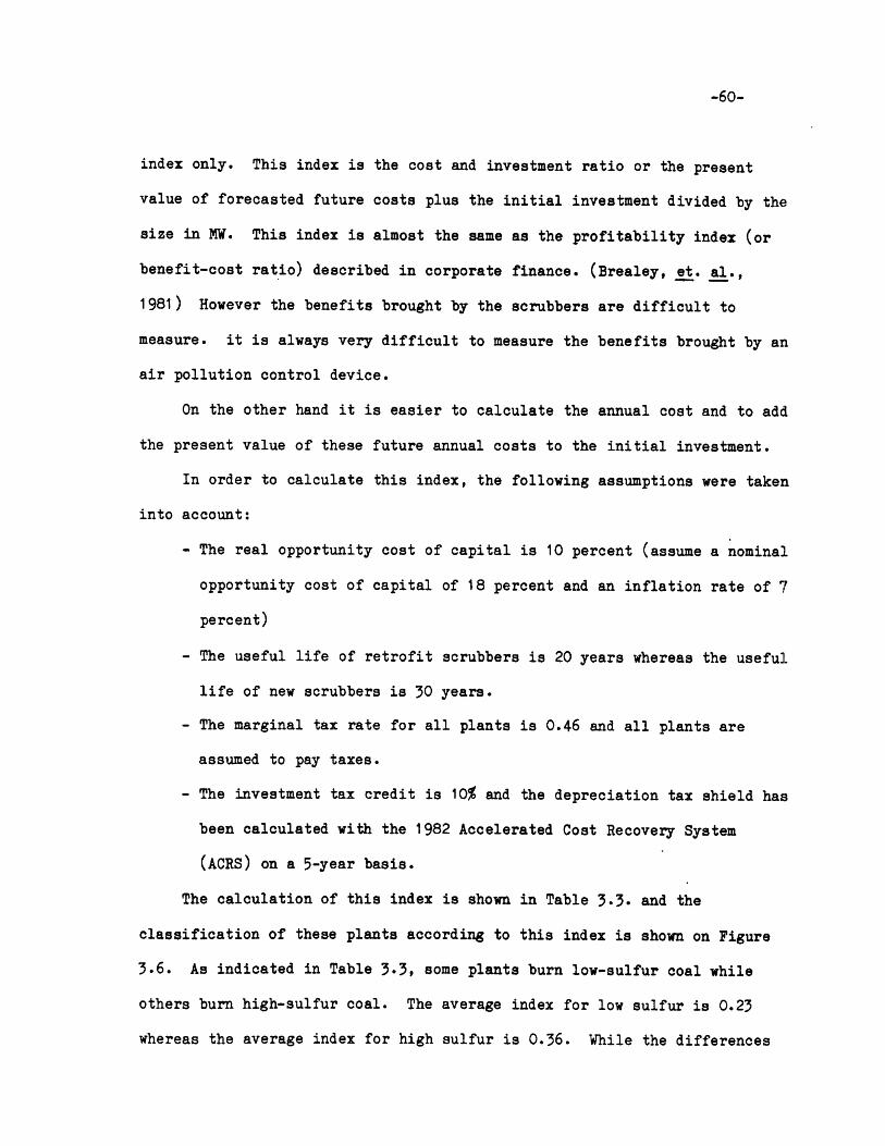
index only. This index is the cost and investment ratio or the present
value of forecasted future costs plus the initial investment divided by the
size in MW. This index is almost the same as the profitability index (or
benefit-cost ratio) described in corporate finance. (Brealey, et. al.,
1981) However the benefits brought by the scrubbers are difficult to
measure. it is always very difficult to measure the benefits brought by an
air pollution control device.
On the other hand it is easier to calculate the annual cost and to add
the present value of these future annual costs to the initial investment.
In order to calculate this index, the following assumptions were taken
into account:
- The real opportunity cost of capital is 10 percent (assume a nominal
opportunity cost of capital of 18 percent and an inflation rate of 7
percent)
- The useful life of retrofit scrubbers is 20 years whereas the useful
life of new scrubbers is 30 years.
- The marginal tax rate for all plants is 0.46 and all plants are
assumed to pay taxes.
- The investment tax credit is 10% and the depreciation tax shield has
been calculated with the 1982 Accelerated Cost Recovery System
(ACRS) on a 5-year basis.
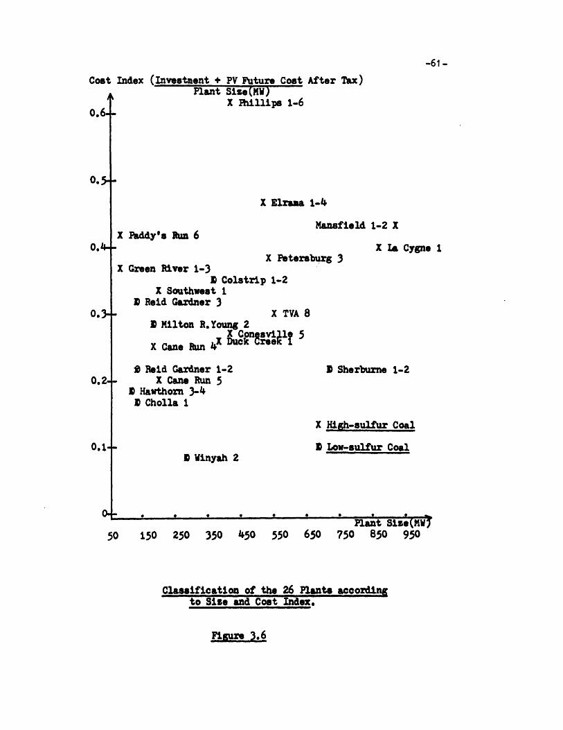
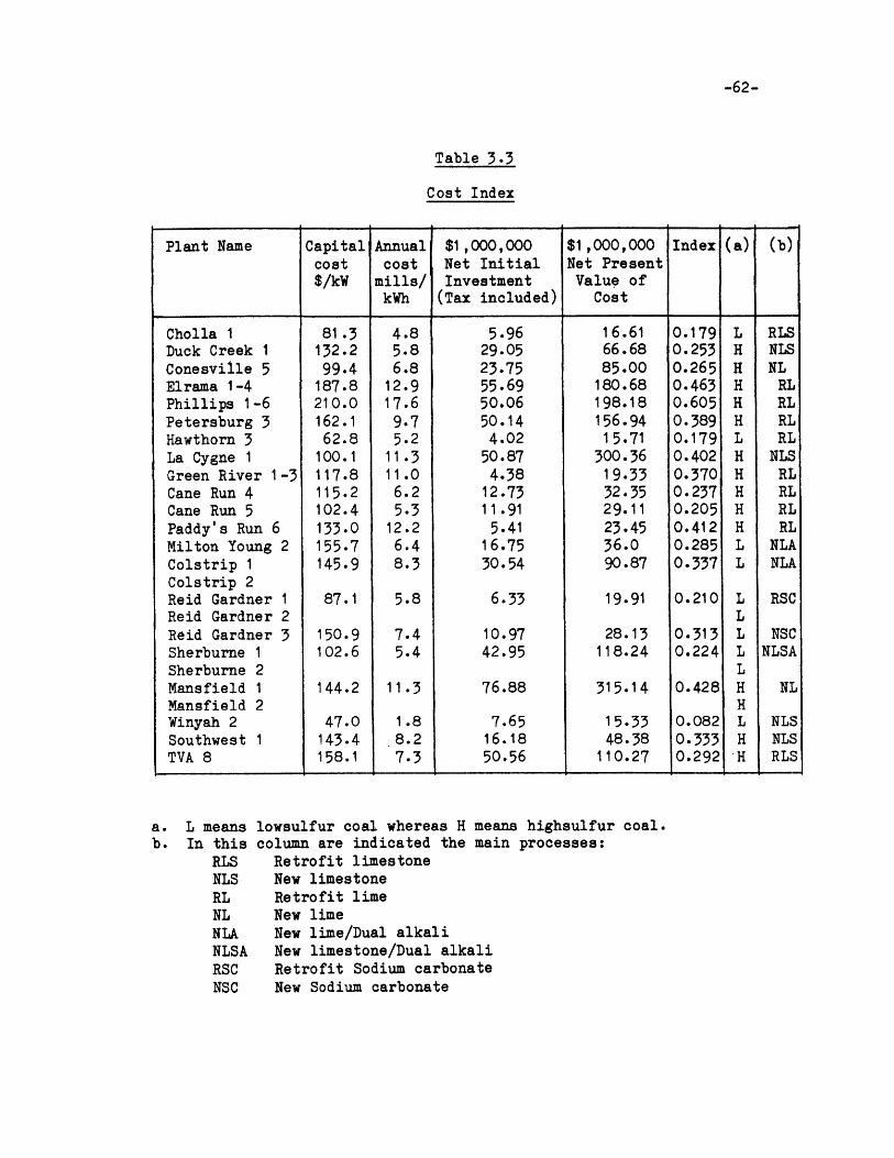
The calculation of this index is shown in Table 3.3. and the
classification of these plants according to this index is shown on Figure
3.6. As indicated in Table 3.3, some plants burn low-sulfur coal while
others burn high-sulfur coal. The average index for low sulfur is 0.23
whereas the average index for high sulfur is 0.36. While the differences
-61 -
Cost Index (Investment + PV Future Cost After Tax)Plant Sie (MW)
X millips 1-0
0.5+
X Elrama 1-4
X Paddy's Run 6
X Green River 1-3
X SouthweaD Reid Gardnez
Mansfield 1-2 X
X Petersburg 3X Ia Cygne 1
E Colstrip 1-2it 1
3'X TVA 8
U Milton R.Young 2
X ConsvCane 5X Cane Ran 16 Duck GreeK I
0 Reid Gardner 1-2X Cane Run 5
U Hawthorn 3-4D Cholla 1
N Winyah 2
D Sherburne 1-2
X High-sulfur Coal
D Low-sulfur Coal
0+ . 2 0 3 0 - 0o
50 150 250 350 450
.0 0 a --
Plant Sie(MW7550 650 750 850 950
Classification of the 26 Plants accordingto Sie and Cost Index.
Figure 3.6
0.3
0.2.-
0.1-
_ 1 11111 1111111 ......... ...I
0,6
-62-
Table 3.3
Cost Index
a. L means lowsulfur coal whereas H means highsulfur coal.b. In this
RLSNLSRLNLNLANLSARSCNSC
column are indicated the main processes:Retrofit limestoneNew limestoneRetrofit limeNew limeNew lime/Dual alkaliNew limestone/Dual alkaliRetrofit Sodium carbonateNew Sodium carbonate
Plant Name Capital Annual $1,000,000 $1,000,000 Index (a) (b)cost cost Net Initial Net Present$/kW mills/ Investment Value of
kWh (Tax included) Cost
Cholla 1 81.3 4.8 5.96 16.61 0.179 L RLSDuck Creek 1 132.2 5.8 29.05 66.68 0.253 H NLSConesville 5 99.4 6.8 23.75 85.00 0.265 H NLElrama 1-4 187.8 12.9 55.69 180.68 0.463 H RLPhillips 1-6 210.0 17.6 50.06 198.18 0.605 H RL
Petersburg 3 162.1 9.7 50.14 156.94 0.389 H RLHawthorn 3 62.8 5.2 4.02 15.71 0.179 L RLLa Cygne 1 100.1 11.3 50.87 300.36 0.402 H NLS
Green River 1-3 117.8 11.0 4.38 19.33 0.370 H RL
Cane Run 4 115.2 6.2 12.73 32.35 0.237 H RLCane Run 5 102.4 5.3 11.91 29.11 0.205 H RL
Paddy's Run 6 133.0 12.2 5.41 23.45 0.412 H RL
Milton Young 2 155.7 6.4 16.75 36.0 0.285 L NLAColstrip 1 145.9 8.3 30.54 90.87 0.337 L NLA
Colstrip 2Reid Gardner 1 87.1 5.8 6.33 19.91 0.210 L RSCReid Gardner 2 LReid Gardner 3 150.9 7.4 10.97 28.13 0.313 L NSCSherburne 1 102.6 5.4 42.95 118.24 0.224 L NLSASherburne 2 LMansfield 1 144.2 11.3 76.88 315.14 0.428 H NLMansfield 2 HWinyah 2 47.0 1.8 7.65 15.33 0.082 L NLSSouthwest 1 143.4 .8.2 16.18 48.38 0.333 H NLSTVA 8 158.1 7.3 50.56 110.27 0.292 H RLS
-63-
between the new and retrofit scrubbers decrease with the cost index
(because different useful lifes are considered), the limestone process
still remains cheaper and it is cheaper to install a scrubber on a plant
which burns low-sulfur coal than to install a scrubber on a plant which
burns high-sulfur coal.
3.3.6 Conclusion
Several studies or forecasts of the cost of FGD technology were made
within the last ten years. It is interesting to compare the results
obtained with our results.
In 1973, the Sulfur Oxide Control Technology Assessment Panel (U.S.
Environmental Protection Agency, 1973) estimated the costs of six different
sulfur oxide control technologies. The investment per kilowatt of capacity
ranged from $17 to $65, and the operating costs ranged from 0.6 mills to 3
mills per Kilowatt hour. At the time these costs were estimated, they
represented a large fraction, ranging from 20 percent upward, of the total
cost of electricity generation. These costs were estimates and were not
based on actual data.
An attempt to produce a generalized cost function has been made by
Burchard, (Burchard, 1972) who used data from a number of cost studies for
sulfur dioxide scrubbing systems and developed equations to represent costs
under a variety of conditions. Although it is not clear that Burchard's
equation is actually fitted by regression techniques to the existing data,
he does use his equation to reestimate the cost of actual facilities in his
-64-
input data and finds that his cost estimates are within 15 percent of the
original estimates.
A notable feature of Burchard's equation and data is the tremendous
range in most of the cost variables, many of which vary by at least a
factor of 2. The major contribution of this cost function is to reconcile
the variety of cost estimates for different scrubbing installations, which
vary enormously in parts because of the tremendously varied conditions of
plant size, fuel sulfur content, byproduct, disposal costs, and a number of
other factors.
Methods for sulfur dioxide removal from stack gases have been known in
principle for some time, but only during the last decade have large-scale
installations been made that can lead to the development of improvements
and cost reductions in this technology. If policies are adopted that
encourage or force the installation of large numbers of sulfur dioxide
scrubbers over the future, it would be reasonable to expect that research
and development would lead to substantial improvements in these processes.
Maximum efficiencies should rise and costs should fall.
All this cost analysis is concerned by the tail-end treatment or
removal of sulfur dioxide from stack gases. It is also possible to reduce
sulfur dioxide emisions, by removing sulfur from the fuel before it is
burned, by burning a low-sulfur fuel. Depending upon market conditons, in
some cases it may be less expensive to purchase low-sulfur coal than it is
to install stack gas scrubbers (See Section 1.2). Thus cost estimates
based upon gas stack scrubbing alone are likely to overestimate actual
costs incurred in a cost-minimizing abatement program for an area or a
country.
-65-
4 FUNCTIONAL ANALYSIS OF PROVEN FGD
4.1 Introduction
The cost analysis described in Section 3 would not be sufficient
without a functional analysis. One of our assumptions was a continuous
operation of the boiler and a capacity factor of 65%. Therefore the prices
calculated in Section 3 might not be realistic. A very high annual cost
might result from a very low utilization of the scrubber. On the other
hand, a very low annual cost might result from a very high utilization.
In order to remedy these drawbacks, we will study how well the FGD
systems operate and what are the main reasons for failure.
Section 4.2 contains an overview of the proposed methodology. A
definition of different viability indexes is given and the way these data
are collected is explained.
In Section 4.3, the results obtained by applying this methodology are
shown. The four main processes are compared with the set of indexes
previously described. The evolution of one of these indexes, the
operability, is shown. The different regulatory classes are presented and
a study of the operablity limit shows how well the legislation is applied.
After an analysis of the main reasons for failure, an interpretation of the
applied results is given.
Section 4.4 constitutes a synthesis of the results obtained in Section
4 and Section 3. The definition of the operating cost is given. Then the
average cost curve can be drawn.
Finally in Section 4.5 improvements of the viability of the FGD
systems are suggested as well as other methods of sulfur removal.
-66-
4.2 Description of the Methodology
4.2.1 Definition of Different Viability Indexes
Several parameters have been developed to quantify the viability of
FGD system technology. The operation of any FGD system during a given
period can be accurately represented by the "availability," "reliability,"
"operability," and "utilization" indexes. These parameters are defined
below and discussed briefly.
The availability index (A) is defined as the number of hours the FGD
system is available for operation (whether operated or not) divided by the
number of hours in period (8760 hrs for a year), expressed as a percentage:
A(%) = available FGD hrsx 100hrs in period
This parameter tends to overestimate the viability of the FGD system
because it does not penalize for election not to operate the system when it
could have been operated. Boiler downtime may tend to increase the
magnitude of the parameter because FGD failures generally cannot occur
during such periods.
The reliability index (R) is defined as the number of hours the FGD
system was operated divided by the number of hours the FGD system was
called upon to operate, expressed as a percentage:
R(%) = actual FGD hrs x 100.Called upon FGD hrs
This parameter has been developed in order not to penalize the FGD
- I...mE*IIII1 .IIIhI&II
system for elected outages, periods when the FGD system could have been run
but was not run because of chemical shortages, lack of manpower, short
duration boiler operations, etc. The main problem in using this formula is
the concise determination of whether the system was "called upon to
operate" during a given time period. Moreover, an undefined value can
result when the FGD system is not called upon to operate for a given period
(for instance, turbine or boiler outage when the FGD system is available).
The operability index (0) is defined as the number of hours the FGD
system was operated divided by the number of hours the boiler was operated,
expressed as a percentage:
0(%) = actual FGD hrsactual boiler hrs
This parameter indicates the degree to which the FGD system is
actually used, relative to boiler operating time. The parameter is
penalized when options are exercised not to use the FGD system when the
system is operable. In addition, an undefined value can result when the
FGD system is not called upon to operate for a given period (f6r instance,
turbine or boiler outage when the FGD system is available) (See
reliability).
The utilization index (U) is defined as the number of hours the FGD
system was operated divided by the number of hours in period (8760 hrs for
a year), expressed as a percentage:
U(%) * actual FGD hrs x 100hrs in period
-68-
This parameter is a relative stress factor for the FGD system. It is
not a complete measure of the FGD system viability because the parameter
can be strongly influenced by conditions that are external to the FGD
system. Infrequent boiler operation will lower the value of the parameter
although the FGD system may be highly dependable in its particular
application.
4.2.2 Collection of the Data
The four indexes mentioned above have been reported monthly and
supplied voluntarily by utility representatives, FGD system suppliers and
designers, regulatory agencies and others. These FGD system design and
performance data have been collected in a computerized data base known as
the Flue Gas Desulfurization Information System (FGDIS). Neither the U.S.
Environmental Protection Agency (EPA) nor the designated contractor
warrants the accuracy or completeness of information contained in this data
base.
The information provided for this thesis comes from a report which
summarized the data from the data base. (Bruck et. al., 1981)
Among the four indexes reported, only the last two can be actually
checked because both the number of actual FGD hours and the number of
actual boiler hours are also reported. As a matter of fact, the reported
operability and utilization indexes have not been taken into account. They
were recalculated from the numbers of hours indicated.
The reliability and operability indexes can be easily compared since
-69-
they only differ by the value of their denominator. It seems clear that
when the boiler does not operate, the FGD system should not operate either.
Therefore the number of hours the FGD system is called upon to operate
should be less than the number of actual boiler hours, which means that the
reliability should be greater than the operability. However, the contrary
can be noticed for a few utilities. As mentioned above, it depends on the
definition of "called upon to operate". Since the number of hours the FGD
system was called upon to operate and since the number of available FGD
hours are not recorded, the availability and reliability indexes cannot be
trusted as much as the operability and utilization indexes.
It will also be noticed that for some other reasons such as strike or
personnel change, the numbers recorded are either unavailable for a given
period or not recorded the same way they were before.
All these considerations have been taken into account so that the
following analysis could be as reliable as possible.
4.3 Results and Interpretations
4.3.1 Comparison of the Different Viability Indexes in 1980 or 1981
The utilization, operability, reliability and availability were
calculated for the group of plants already analyzed in Section 3. The
method of calculation is explained in the Appendix. The results are
presented in Table 4.1. The capacity factor is also included.
The distribution curve of the utilization index has been drawn on
Figure 4.1. The retrofit scrubbers are not used as much (55%) as the new
Irili1 Irili
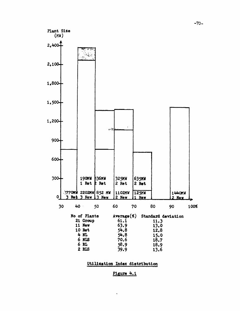
Plant Size(MW)
2, 4 00--
2,100-
1,800 -
.5004-
1,200+
900+
6004-
300- - 190MW1 Ret
. ,770MW 2202MW0 3 Ret 3 New
30 40
No of Plants21 Group11 New10 Ret4 NL6 NLs6 RL2 RLS
50 60 70 80 90 100%
Average(%) Standard deviation61.1 11,363.9 13,054.8 12.854.8 15.070.6 18.758.9 18.939.9 13.6
Utilisation Index distribution
Figure 4.1
-70-
536MW. Ret
852 MW,3 New
635MW2 Ret
i125MWiI New
325MW2 Ret
1102MW2 New
1440nw2 New
12 No v I
CI
r

1 # t ,.a
Table 4.1
Viability Indexes in 1980 and 1981
New Start- MW Process Utiliz Operab reliab availab cap FactPlant Name Ret Up Date
Cholla 1 R 10/73 126 limestone 55.4 72.7 99.81 99.82 87.1Duck Creek 1 N 7/76 378 limestone 52.5 72.7 82.0 58.9 62.9Conesville 5 N 1/77 411 lime 49.6 88.9 93.1 82.2 83.3Elrama 1-4 R 10/75 510 lime 72.2 78.7 94.2 95.4 49.0Phillips 1-6 R 7/73 410 lime 58.5 64.3 73.5 74.6 50.5Petersburg 3 N 12/77 532 limestone NA NA NA NA NAHawthorn 3 R 11/72 110 lime 35.9 100 97.0 93.0 25.8Hawthorn 4 R 8/72 110 lime 36.7 100 93.9 85.6 45.3La Cygne I N 12/72 874 limestone 45.1 98.1 93.7 85.9 45.6Green River 1-3 R 9/75 64 lime NA NA NA 100 NACane Run 4 R 8/76 190 lime 49.3 85.8 92.1 79.0 39.8Cane Run 5 R 12/77 200 lime 60.0 90.8 94.3 86.1 45.2Paddy's Run 6 R 4/73 70 lime NA NA NA 100 NAMilton R. Young 2 N 9/77 185 lime A 66.3 78.6 90.1 74.4 83.2Colstrip I N 9/75 360 lime A NA NA NA 89.3 NAColstrip 2 N 5/765 360 lime A NA NA NA 88.4 NAReid Gardner 1 R 3/74 125 SC 76.5 93.3 93.1 93.6 96.8Reid Garnder 2 R 4/74 125 SC 62.0 94.3 96.5 97.5 95.3Reid Gardner 3 N 6/76 125 SC 70.4 98.2 95.4 87.2 88.5Sherburne 1 N 3/67 720 limestone A 95.3 100 100 100 71.2Sherburne 2 N 3/77 720 limestone A 96.3 100 100 100 72.6Bruce Mansfield 1 N 12/75 917 lime 45.5 100 NA 77.8 NABruce Mansfield 2 N 7/77 917 lime 63.9 100 NA 95.9 NAWinyah 2 N 7/77 280 limestone A 58.5 93.5 94.0 85.9 69.8Southwest 1 N 4/77 194 limestone A 51.2 74.5 85.7 63.3 63.3TVA 8 R 5/77 550 limestone A 36.4 80.7 NA 90.6 41.0
(NA = Not Available)
-72-
ones (64%). The limestone process installed on new plants (NLS) has a very q
high utilization index (70%). In Section 3, the same NLS category obtained
the lowest annual cost in mills per kWh. However, as was explained in
Section 4.2.1 this index can be strongly influenced by conditions that are
external to the FGD system. This is the reason why we must consider the
other indexes.
The distribution curve of the operability index has been drawn on
Figure 4.2. The operability index is definitely higher (95%) for FGD
systems installed on new plants than for FGD systems installed on old
plants (83%). However the lime process installed on new plants has now the
highest operability index. Nothing can really be concluded about the
processes. Whereas the difference of operability between the new and
retrofit scrubbers is high (more than 10%), the difference of operability
between the lime and limestone processes, on either old or new plants is
very low (2 or 3%). In section 4.3.3, an explanation of these results is
given.
The distribution curve of the reliability index has been drawn on
Figure 4.3. Only 18 plants gave values of reliability indexes. It mainly
comes from the difficulty to define what is meant by "called upon to
operate". The differences between new and retrofit scrubbers, as well as
between lime and limestone processses are not very important.
The reliability index is the highest of the four indexes. Its average
value (93%) is also very high. For the lime processes installed on new
plants (NL), the reliability is lower (92%) than the operability (97%). As
mentioned in Section 4.2.2 the operability should be lower than the
reliability. The contrary means that the FGD system was called upon to
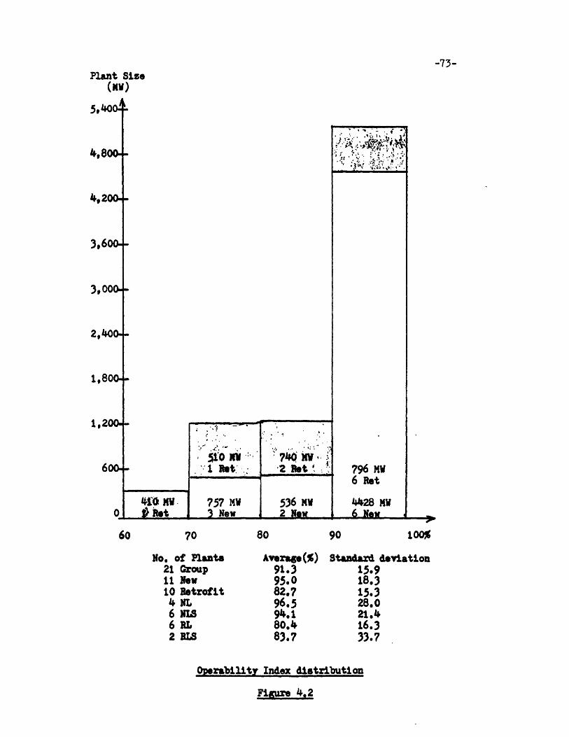
-73-Plant Size
(xV)
1,8
796 MW6 Ret
4428 MW
60 70 80 90 lo0%
No. of Plants21 Group11 New10 Retrofit4 NL6 NLS6 RL2 ELS
Average(%)91.395.082.796.594,.180.483.7
Standard deviation15.918.315.328.021.416.333.7
Operability Index distribution
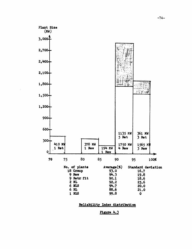
-74-
Plant Sise(MW)
3, ooo00
2,7
2,700--
2,100--
1,800-
1,50 -
1,200- -
900- -
600- -
300--410 0 Ret
01 A
378 MW1 New 194 MW
1 New
70 75
No. of plants18 Group
9 New9 Retr fit2 NL6 NLS6 RL1 RLS
Average(%)93.094.390. 192.294.788.699.8
Standard deviation16.719.818.625.620.021.0
0
Reliability Index distribution
M 4
1135 MW5 Ret
1750 MW4 New
361 MW3 Ret
1565 mlM3 New
80 1oo%
- _ r---rx.--~----X~ ~-- PII-S=i~E ~---pPs ~; ~__~ _~__~
__
__ _ __ _ _ __ _ _ __ _ InMm IIilfi Iih A,
-75-
operate when the boiler was not operating. It might be a way of keeping
the FGD system in operation in order to avoid the formation of sludges.
The distribution curve of the availability index has been drawn on
Figure 4.4. Contrary to the three former indexes, the availability of the
retrofit scrubbers is greater than the availability of the new scrubbers.
This result is only surprising in appearance. If the boiler does not
operate most of the time, the risk of FGD failure is very low and therefore
the availability of the system is very high. This is the reason why we
must also consider the utilization index when we look at the availability.
We already saw that the utilization index is a lot lower for retrofit
scrabbers than for new scrubbers and this is the reason why we observe this
amazing result.
Finally the distribution curve of the capacity factor has been drawn
on Figure 4.5. This capacity factor is the capacity factor of the boiler
and does not measure the viability of the FGD system. However a comparison
of this curve with the FGD utilization curve can be made. The average
capacity factor is the same as the average utilization factor - 61%.
Whereas the capacity factor of a new boiler (67%) is greater than the
utilization factor of a new scrubber (64%), the capacity factor of an old
boiler (52%) is less than the utilization factor of a retrofit scrubber
(55%). Nothing can be concluded from this comparison because these two
indexes are really independent.
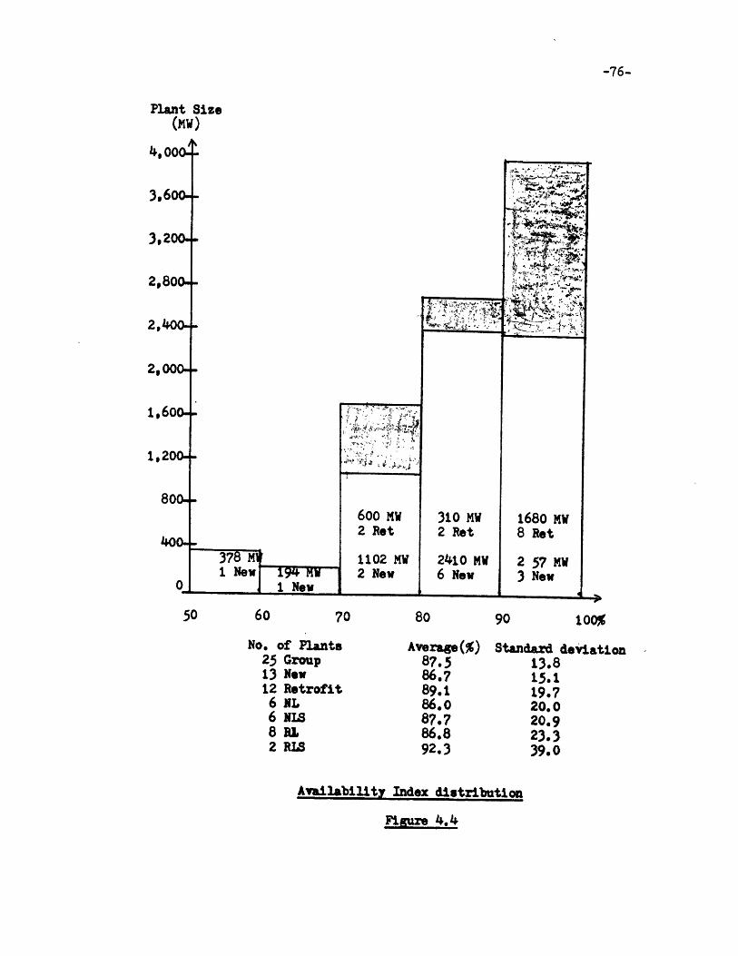
Plant Size(MV)
4,0001
3,6004
3,20-
2,80
2,0
2,00
1,60
1,20
800-4
403I New 194 MW
1 New,ThneU r
600 MW2 Ret
1102 MW2 New
No. of Plants25 Group13 New12 Retrofit6 NL6 NLS8 RL2 RIS
Average(%)87.586,789.186.087.786.892.3
Standard deviation13.815.119.720.020.923.339.0
Availability Index distribution
-76-
1680 MW8 Ret
2 57 MW3 New
310 MW2 Ret
2410 MW6 New
100%
- -- p-rrrl C-=--F~CI ~Ccr=ii~= -- ~F-4LI-;W-~_I________
I ~I
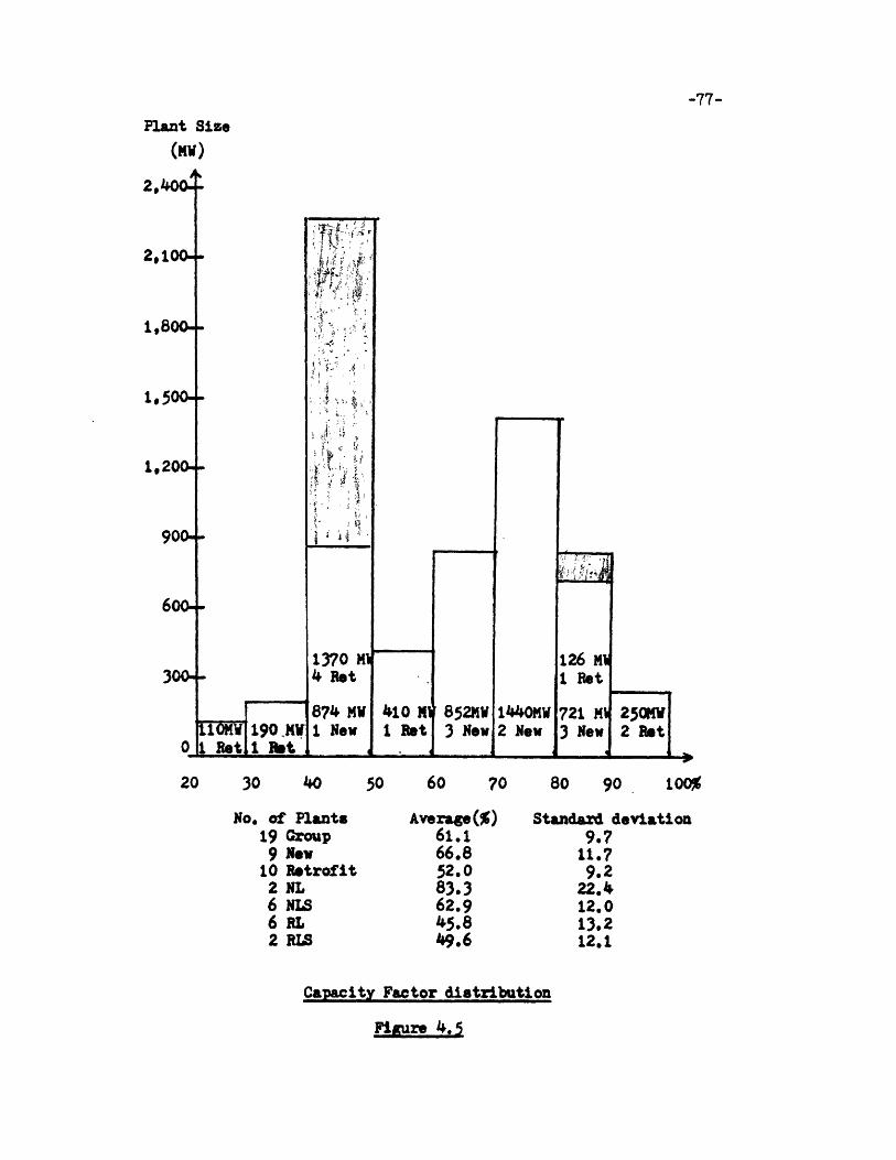
-77-
Plant Sise
(MW)
20 30 40 50 60 70 80 90 10oo%
No. of Plants Average(%) Standard deviation19 Group9 New
10 Retrofit2 NL6 NS6 RL2 RLS
61.166.852.083.362.945.849.6
9.711.79.2
22.A12.013.212.1
Capacity Factor distribution
PFigure 4.5
I
-78-
4.3.2 Evolution of the Operability
Among the four viability indexes described in Section 4.2.1, the
operability seems the most reliable since the number of hours the FGD
system is operated is recorded by the utility as well as the number of
boiler hours. It also gives an accurate measure of the viability of the
FGD system. That is the reason why this index has been chosen to analyze
the viability of the FGD systems through the years.
The results are shown in Table 4.2. The years of FGD operation begin
only after the commercial start-up. Four plants, Hawthorn 3 & 4, La Cygne
1 and Paddy's Run 6 have been operating for nine years. The value 0 was
given to the operability whenever both the number of boiler hours and FGD
hours were equal to zero, which was a case of indetermination.
The average operability has been calculated for every year and drawn
on Figure 4.6. During the first three years the operability stays at a low
level of about 60% before jumping at the fourth year and reaching during
the following years an asymptotic level of about 95%.
The average operability was also calculated for the four different
categories of processes, new lime, new limestone, retrofit lime, and
retrofit limestone scrubbing. It is interesting to look at the curve of
the NL category. The shape is about the same as the average operability.
However the level of the first years is lower at about 30% and the
asymptotic level is lower at about 80%. The precipitation of calcium
sulfate or gypsum can explain this low level of operability.
The shape of the average operability curve can be compared to the S-
shaped curve of the spread of innovation described by many economists.
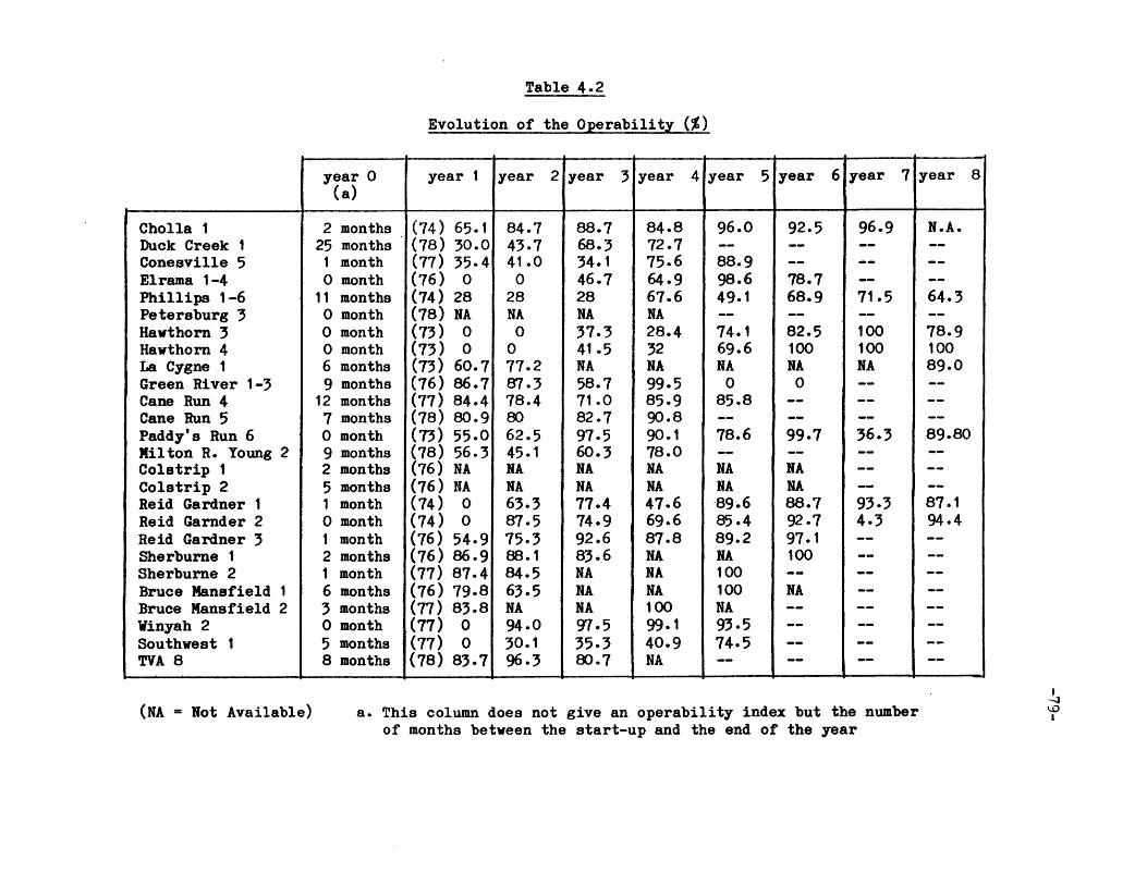
$ ." . L
Table 4.2
Evolution of the Operability (%)
Cholla 1Duck Creek 1Conesville 5Elrama 1-4Phillips 1-6Petersburg 3Hawthorn 3Hawthorn 4La Cygne 1Green River 1-3Cane Run 4Cane Run 5Paddy's Run 6Milton R. Young 2Colstrip 1Colstrip 2Reid Gardner 1Reid Garnder 2Reid Gardner 3Sherburne 1Sherburne 2Bruce Mansfield 1Bruce Mansfield 2Winyah 2Southwest 1TVA 8
year 0(a)
2 months25 months1 month0 month
11 months0 month0 month0 month6 months9 months
12 months7 months0 month9 months2 months5 months1 month0 month1 month2 months1 month6 months3 months0 month5 months8 months
N 2 a a a a 4 £
year 1
-r-
(74)(78)(77)(76)(74)(78)(73)(73)(73)(76)(77)(78)(73)(78)(76)(76)(74)(74)(76)(76)(77)(76)(77)(77)(77)(78)
year
65.130.035.4
028NA
0O
60.786.784.480.955.056.3NANA
OO
54.986.987.479.883.8
0O
83.7
year
88.768.334.146.728NA37.341.5NA58.771.082.797.560.3NANA77.474.992.683.6NANANA97.535.380.7
year 4
84.872.775.664.967.6NA28.432NA99.585.990.890.178.0NANA47.669.687.8NANANA10099.140.9NA
year
96.0
88.998.649.1
74.169.6NA0
85.8
78.6
NANA89.685.489.2NA100100NA93.574.5--
year
92.5
78.768.9
82.5100NA0
99.7
NANA88.792.797.1100
NA----
--
year 7
96.9
71.5
100100NA
36.3
93.34.3
,-
m----------
(NA = Not Available) a. This column does not give an operability index but the numberof months between the start-up and the end of the year
year
N.A.--
o--
64.3
78.910089.0
89.80
--
87.194.4--------
----
..
84.743.741.0028NA0077.287.378.48062.545.1NANA63.387.575.388.184.563.5NA94.030.196.3
... -- -- --
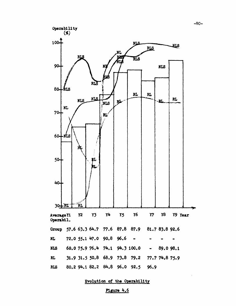
-80-Operability
M%
AverageYi Y2Operabil.
Group 57.6 63.3
NL 72.0 55.1
NLs 60.0 75.9
RL 31.9 31.5
R.LS 80.2 94.1
Y3 Y1 Y5 Y6 Y7 Y8 Y9 Year
64.7
47.0
76..
50.8
82.2
77.6
90.8
68.9
84.8
87.8
96.6
94.3
73.8
96,0
87.9
100.0
79.2
92.5
81.7 83.8 92.6
- 89.0 98.1
77.7 74.8 75,9
96.9
Evolution of the Operability
Figure 4.6
-81-
(Kennedy et. al., 1972) This curve shows that most innovations exhibit a
slow initial acceptance, a period during which many firms adopt the
innovation and a final stage in which adoption ceases (at perhaps less than
100%). The meaning is slightly different. The percent of firms adopting
the FGD technology does not change since we are studying our 26 utility
plants. However it represents the evolution of technical progress and
shows how fast the utilities master the FGD technology.
4.3.3 Regulatory Classes and Operability Limit
The sulfur emissions are regulated by standards set up by the
Environmental Protection Agency (EPA) and called the New Source Performance
Standards (NSPS). These standards, promulgated in December 1971 and in
June 1979, are more stringent for new plants than for old plants.
Depending on the plant location and the quality of coal used, the plant
belongs to one of the following categories:
A The unit is subject to NSPS promulgated in June 1979.
B The unit is subject to NSPS promulgated in December 1971.
C The unit is subject to standards more stringent than 79 NSPS.
D The unit is subject to standards more stringent than 71 NSPS, but
no more stringent than 79 NSPS.
E The unit is subject to standards equal to or less stringent than 71
NSPS.
These categories are shown on Table 4.3. These data were provided by
PEDCo. For each plant are given both the regulatory classification and the
11 11I III I IJ11 1 I1,1 1 IIIII IIIJI 11611, 11 1 1, .1 1 IIIEW
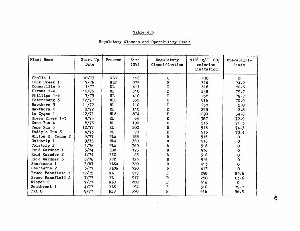
Table 4.3
Regulatory Classes and Operability Limit
Plant Name Start-Up Process Size Regulatory x10 9 g/J S02 OperabilityDate (MW) Classification emission limit
limitation
Cholla 1- 10/73 RLS 126 C 430 0Duck Creek 1 7/76 NLS 378 B 516 74.2Conesville 5 1/77 NL 411 D 516 80.6Elrama 1-4 10/75 RL 510 D 258 79.7Phillips 1-6 7/73 RL 410 D 258 79.7Petersburg 3 12/77 NLS 532 B 516 70.9Hawthorn 3 11/72 RL 110 D 258 2.8Hawthorn 4 8/72 RL 110 D 258 2.8La Cygne 1 12/71 NLS 874 E 1290 59.6Green River 1-3 9/75 RL 64 E 387 72.9Cane Run 4 8/76 RL 190 D 516 74.3Cane Run 5 12/77 RL 200 D 516 74.3Paddy's Run 6 4/73 RL 70 E 516 70.4Milton R. Young 2 9/77 NLA 185 D 516 0Colstrip 1 9/75 NLA 360 B 516 0Colstrip 2 5/76 NLA 360 B 516 0Reid Gardner 1 3/74 RSC 125 B 516 0Reid Garnder 2 4/74 RSC 125 B 516 0Reid Gardner 3 6/76 NSC 125 B 516 0Sherburne 1 3/67 NLSA 720 D 413 0Sherburne 2 3/77 NLSA 720 D 413 0Bruce Mansfield 1 12/75 NL 917 D 258 83.6Bruce Mansfield 2 7/77 NL 917 D 258 83.6Winyah 2 7/77 NLS 280 B 516 0Southwest 1 4/77 NLS 194 B 516 75.7TVA 8 5/77 RLS 550 E 516 96.5
1 . 1 1 t
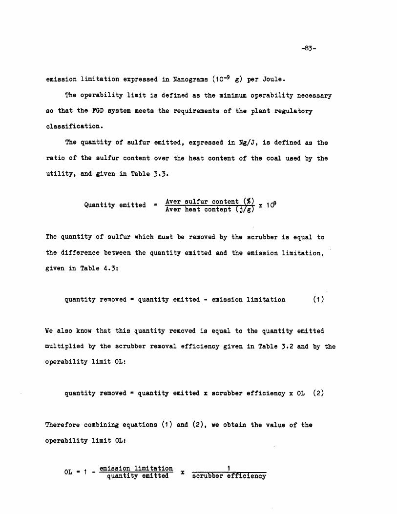
___________________________________________________ im InIIIIuIIIInII mrnmIIIIhIIImYI ImMNY1ImI
-83-
emission limitation expressed in Nanograms (10-9 g) per Joule.
The operability limit is defined as the minimum operability necessary
so that the FGD system meets the requirements of the plant regulatory
classification.
The quantity of sulfur emitted, expressed in Ng/J, is defined as the
ratio of the sulfur content over the heat content of the coal used by the
utility, and given in Table 3.3.
Quantity emitted = Aver sulfur content (%)Aver heat contept (j/g)
The quantity of sulfur which must be removed by the scrubber is equal to
the difference between the quantity emitted and the emission limitation,
given in Table 4.3:
quantity removed = quantity emitted - emission limitation (1)
We also know that this quantity removed is equal to the quantity emitted
multiplied by the scrubber removal efficiency given in Table 3.2 and by the
operability limit OL:
quantity removed - quantity emitted x scrubber efficiency x OL (2)
Therefore combining equations (1) and (2), we obtain the value of the
operability limit OL:
emission limitation 1quantity emitted scrubber efficiency
-- -
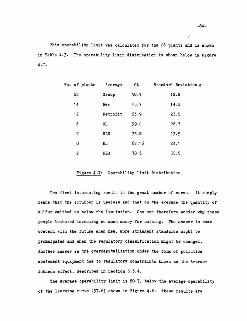
-84-
This operability limit was calculated for the 26 plants and is shown
in Table 4.3. The operability limit distribution is shown below in Figure
4.7.
No. of plants Average OL Standard Deviation a
26 Group 50.7 12.8
14 New 45.7 14.8
12 Retrofit 63.9 23.5
6 NL 59.2 26.7
7 NLS 35.8 13.9
8 RL 67.16 24.1
2 RLS 78.5 55.5
Figure 4.7: Operability Limit Distribution
The first interesting result is the great number of zeros. It simply
means that the scrubber is useless and that on the average the quantity of
sulfur emitted is below the limitation. One can therefore wonder why these
people bothered investing so much money for nothing. The answer is some
concern with the future when new, more stringent standards might be
promulgated and when the regulatory classification might be changed.
Another answer is the overcapitalization under the form of pollution
abatement equipment due to regulatory constraints known as the Averch-
Johnson effect, described in Section 3.3.4.
The average operability limit is 50.7, below the average operability
of the learning curve (57.6) shown in Figure 4.6. These results are
-85-
apparently good, However, a closer look is necessary. When not zero, the
operability limit is included between 70 and 95%, numbers usually reached
by the fourth year of utilization (See Figure 4.6). Moreover the RL
category whose learning curve is well below the average learning curve
(-20%) has one of the highest operability limits (67.6). In 1981, 5 FGD
systems representing 25% of the MW capacity had operability indexes below
their operability limits. The conclusion is quite disappointing. Whenever
the scrubbers are useless the present operability is very high whereas
whenever the emission limitations depend on the operability, this index is
generally below the limit.
4.3.4 Main Reasons for Failure
The main reasons for failure are the freeze of the make-up solution,
the plugging of the lines and the corrosion of different parts of the FGD
system. (Chem Systems International Ltd., 1976)
In the winter months, when the weather conditions are particularly
bad, a utility experiences some problems due to frozen pipes. Although it
does not endanger the scrubber nor its components, the freeze decreases the
level of operability and is difficult to prevent. That is the reason why
the operability index does not go over 92%. Moreover the capacity factor
of the plant is generally the highest during these winter conditions
because the demand for electricity reaches its peak. While the scrubber
cannot operate because of the weather, the boiler operates much more than
usual and thus a bigger quantity of sulfur is emmitted to the atmosphere.
-86-
The plugging of the lines has been reported by almost all the
utilities which operate a FGD system. This generally occurs during the
first years of operation. While the firm moves along the learning curve,
these problems are progressively solved.
A certain level of solids must be maintained in the slurry. Thus the
precipitation of gypsum and the calcium sulfite/sulfate solid solution
occurs. However the system must be kept below the critical level of
saturation with respect to gypsum.
Another parameter, the pH, has an important impact on scaling. A high
pH promotes the formation of scale whereas a low PH reduces the sulfur
dioxide removal. Optimum levels of 8 for lime and 6 for limestone have
been determined by operating experience.
Corrosion seems to be a very important problem in the FGD systems.
Even if'in the short therm it does not cause a decrease of the operability
index, it will on a longterm basis. Sulfurs containing acids and chlorides
are the main agents of corrosion. Elimination of scale in the system
reduces potential sites for locally high concentrations of chloride ion.
The scrubber shells are now made of stainless steel instead of carbon steel
because of its superior resistance to corrosion.
Although the scaling and corrosion problems are solved when the
utility moves along the operating curve, the freeze problem still remains.
Dry scrubbing may be a solution.
-87-
4.3.5 Other Performance Indexes
A good way of comparing the performance of our plants is to plot the
operability versus the operability limit, as shown in Figure 4.8. The
average operability of the points situated on the left side of this Figure
is 96.55 for an average operability limit of 0.23 which gives a very high
ratio of 420. On the right side of the Figure the points represent an
average operability of 88.8 and an average operability limit of 78.7 which
gives a low ratio of 1.13. Fortunately this last ratio is greater than 1
which tends to show that the regulations are met on the average even for
high-sulfur coal.
Another way of looking at the performance is to calculate a
performance index that considers SO2 removal efficiency, operability and
capacity factor. A similar index has been described by Yeager. (Yeager,
1978) This index has been calculated in Table 4.5. Figure 4.9 shows a
classification of these plants according to this index.
The results are very different from Yeager's analysis, although the
same plants are considerd. However Yeager plotted the performance index vs
the start-up date which probably means that the FGD availability and
capacity factor are average, calculated since the beginning whereas mine
are just calculated for the year 1981. It can also be noticed that my
index is slightly different since I used the operability instead of the
availability. Section 4.2.1 explained the flaws linked with the use of the
availability.
The distinction between high-sulfur coal and low-sulfur coal brings
opposite results. The average performance index for plants burning high-
_ ___. ________ __~_ ^____
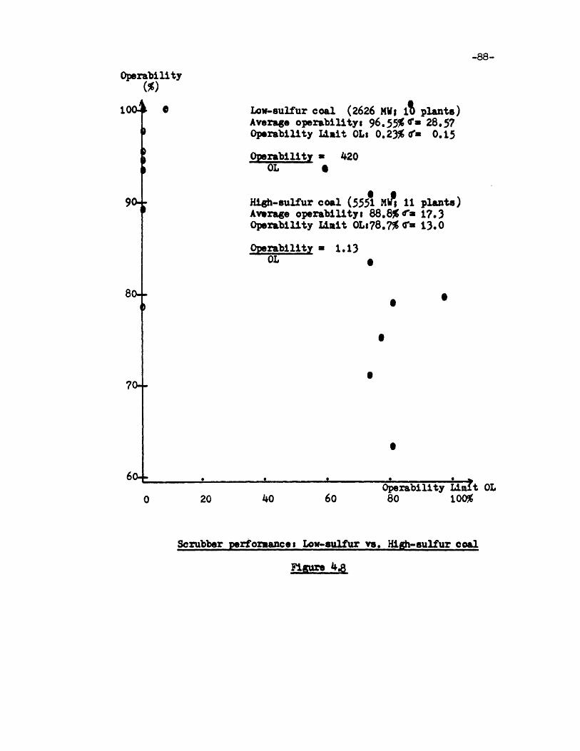
Operability
()
90--
80--
Low-sulfur coal (2626 MWj i plants)Average operability, 96.55% T= 28.57Operability Limait OLs 0.23% 0a 0.15
Operability = 420OL S
High-sulfur coal (5551 MA 11 plants)Average operabilitys 88.8% '. 17.,Operability Liilt OLs78.7%r = 13.0
Operability =OL
1.13
70o
60- 6 0 . 0
Operability80
Limit OL100%
Scrubber performances Low-sulfur vs High-sulfur coal
-88-
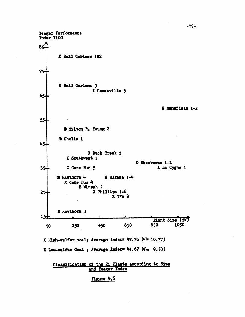
-89-
Yeager PerformanceIndex X100
I Reid Gardner 1&2
P Reid Gardner 3X Coneaville 5
X Mansfield 1-2
N Milton R. Young 2
D Cholla 1
X Duck Creek 1X Southwest 1
X Can* Run 5
3 Hawthorn 4 X B1rana 1-4X Cane Run 4
SVWinyah 2X Phillips 1-6
X TVA 8
M Hawthorn 3
D Sherburne 1-2X La Cygne 1
250 450 650ranx 1r0 pn
850 1050
x High-sulfur coals Average Index= 47.76 (Cu 10.77)
a Low-sulfur coal s Averge Iadex= 41.67 ('= 9.53)
Classification of the 21 Plants according to Siseand Yeager Index
Figure 4.9
8A
65+
55+
454.
35+
25H
4 1, 0
-90-
sulfur coal is 48 whereas it is only 42 for plants burning low sulfur coal.
This suggests a major flaw in the perfomance index. In fact the sulfur
removal efficiency as well the plant capacity factor are factors which
influence the quantity of sulfur removed but not the performance of the
scrubber. The perfomance of the scrubber can be better described by one of
the four indexes described in Section 4.2.1. The Yeager index tries to
unify two incompatible factors: the quantity of sulfur removed and the
actual performance of the scrubber. That is why the Yeager index over-
estimates the actual performance of scrubbers from high-sulfur plants and
underestimates the actual performance of scrubbers from low-sulfur plants.
In order to compare cost and operability the cost index calculated in
Section 3.3.4 can be plotted versus the operability as shown in Figure 4.10.
Although these points are very dispersed, they can be correlated by a
regression whose coefficient of correlation is -0.45 and whose equation is:
Cost Index = 74.55 - (0.5137 x operability)
The Figure simply means that the greater the operability is, the lower
the cost is. This represents an introduction to Section 4.4 where the
relation between operating cost and operability is described.
4.4 Relation Between Operability and Cost
4.4.1 Definition of the Operating Cost
The operating cost represents the direct cost portion of the annual
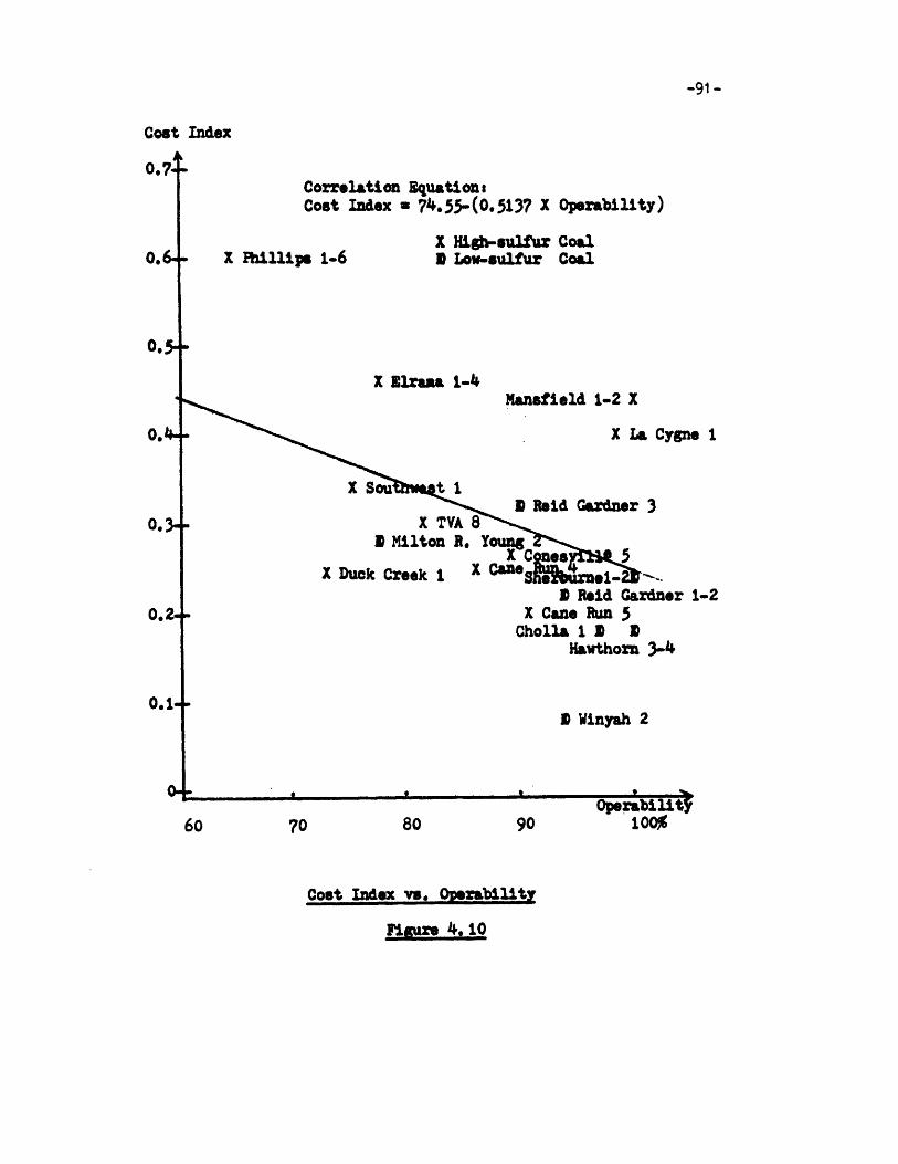
Cost Index
0.7Correlation EquationsCost Index a 74.5-(0o.5137 x Operability)
x Phillips 1-6X High-sulfur CoalSLow-sulfur Coal
x Elraaa 1-4Mansfield 1-2 X
X La C
X Son u 1D Reid Gardner 3
X TVA 83 Milton R. Young
X Duck Creek I X CSae 0.1-D Reid Gardner 1-2
X Cane Run 5Cholla I O D
Hawthorn 3-4
I Winyah 2
uperaOauy100%
Cost Index vs. Operability
Figure 4. 10
-91 -
0.64.
0.,5-
0.3-
ygne I
0.2-
0.1+
60
__
1 C)~JI
0,44
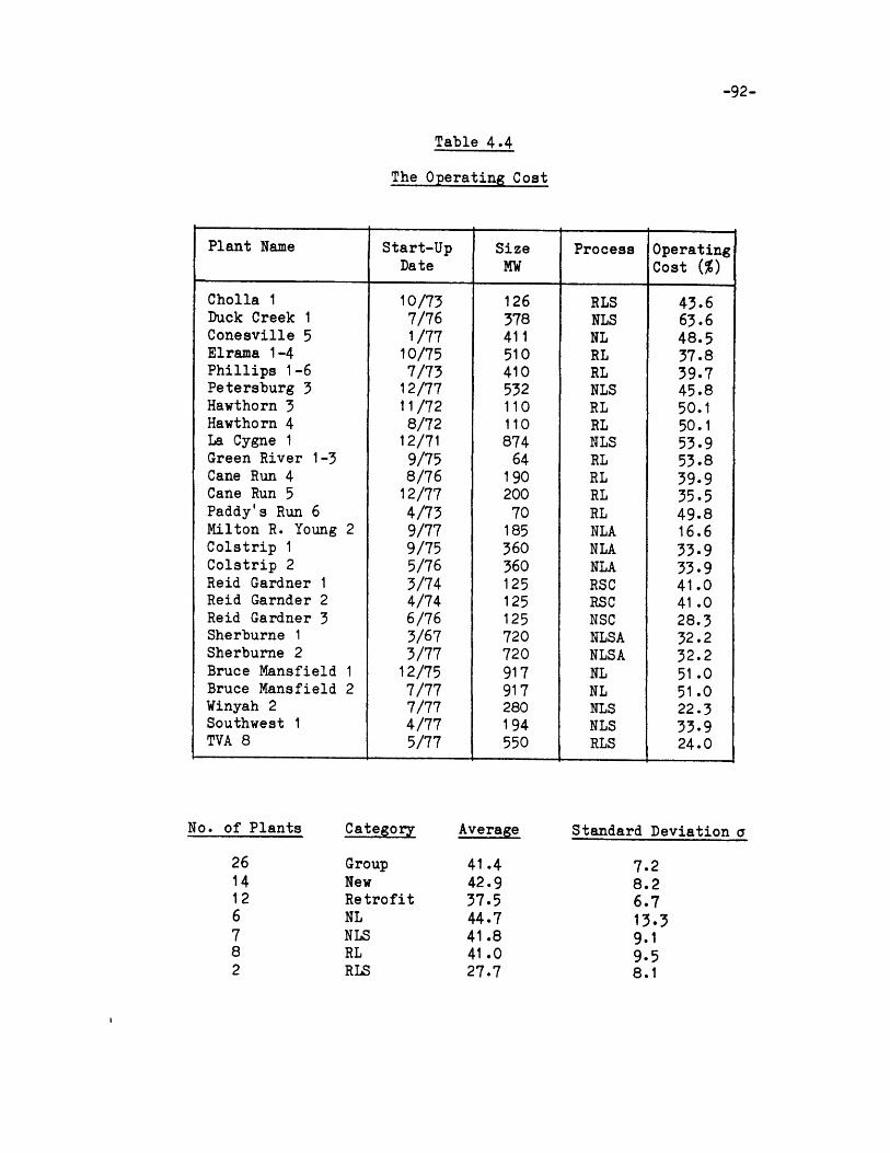
-92-
Table 4.4
The Operating Cost
No. of Plants
2614126782
Category
GroupNewRetrofitNLNLSRLRLS
Average
41.442.937.544.741.841.027.7
Standard Deviation a
7.28.26.713.39.19.58.1
Plant Name Start-Up Size Process OperatingDate MW Cost (%)
Cholla 1 10/73 126 RLS 43.6Duck Creek 1 7/76 378 NLS 63.6Conesville 5 1/77 411 NL 48.5Elrama 1-4 10/75 510 RL 37.8Phillips 1-6 7/73 410 RL 39.7Petersburg 3 12/77 532 NLS 45.8Hawthorn 3 11/72 110 RL 50.1Hawthorn 4 8/72 110 RL 50.1La Cygne 1 12/71 874 NLS 53.9Green River 1-3 9/75 64 RL 53.8Cane Run 4 8/76 190 RL 39.9Cane Run 5 12/77 200 RL 35.5Paddy's Run 6 4/73 70 RL 49.8Milton R. Young 2 9/77 185 NLA 16.6Colstrip 1 9/75 360 NLA 33.9Colstrip 2 5/76 360 NLA 33.9Reid Gardner 1 3/74 125 RSC 41.0Reid Garnder 2 4/74 125 RSC 41.0Reid Gardner 3 6/76 125 NSC 28.3Sherburne 1 3/67 720 NLSA 32.2Sherburne 2 3/77 720 NLSA 32.2Bruce Mansfield 1 12/75 917 NL 51.0Bruce Mansfield 2 7/77 917 NL 51.0Winyah 2 7/77 280 NLS 22.3Southwest 1 4/77 194 NLS 33.9TVA 8 5/77 550 RLS 24.0
-93-
cost as described in Section 3.2.2. This operating cost includes the cost
of raw materials such as lime or limestone, the cost of utilities such as
water and electricity as well as the cost of operating labor, supervision,
maintenance, and repairs.
In Table 4.4 the operating cost has been calculated for each plant of
the group as a percentage of the total annual cost. The average operating
cost represents 41% of the total annual cost.
If the FGD system does not operate during the year the operating cost
will be zero and so will the operability. Therefore the total annual cost
will decrease. On the other hand, the utility which burns coal without
removing sulfur might be obliged to pay a fine. In order to avoid this a
clever strategy can be adopted. A simulation of failures can be performed
and as we saw in Section 4.3 it will be difficult to detect it.
4.4.2 Average Cost Curve
In the former section we saw how the operating cost influences the
operability. The operability directly affects the quantity of sulfur
removed and is thus linked with the price necessary to remove this quantity
by a relation known as the average cost curve.
The average cost curve drawn on Figure 4.11 represents the annual cost
in mills/kWh versus the annual quantity of sufur removed in kg/kWh.
However, this annual cost will be different from the annual cost calculated
in Table 3.2; an average 65% capacity factor and a continuous operation of
the boiler (8760 hrs) were assumed.
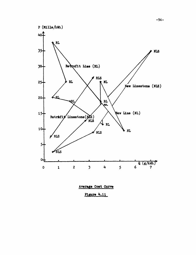
-94-
P (illsAwh)
NLS
.t Line (RL)
New Liiestone (NIS)
Lime (NL)
SnL
i 2 3 S 5 6 (1 2 3 4 5 6 7
Aver e Cost Curve
Figure 4.11
30--
RLS25--
204-
15+
10-NLS
E m
-95-
From the data given by PEDCo, (Bruck et. al., 1981) actual capacity
factors and actual numbers of boiler hours were calculated. The results
are shown in Table 4.5. For five plants, the number of boiler hours is
zero. The demand was too low and the utility did not produce any
elctricity. The capacity factor varies within a range from 25% for
Hawthron 3 to 95% for Reid Gardner 2.
The new price P is calculated as folows;
Pg (mills/kWh) x 0.65 x 8760
capacity factor (%) x number of boiler hours (hrs)
The average operability index was calculated for 1981. The same PEDCo
survey shows the average sulfur content (in percent) and the average heat
content (in J/g) of the coal utilized, and the sulfur design removal
efficiency (in percent) ranging from 45 to 92. These data are listed in
Table 4.5
The quantity of sulfur removed is calculated as follows:
Q(g/KWh) F FGD operability (%) x average sulf. cont. x sulf. eff.average heat cont. (J/g) x 278 10- 9
Two observations can be made from this curve:
- The limestone scrubbing processes have increasing average costs
whereas the lime scrubbing processes have decreasing average costs.
- The curves for new processes, both limestone and lime are situated
on the right side of the Figure, whereas the curves for retrofit
processes are situated on the left side.
The decreasing average cost for the limestone process can be explained
-- ~ MIIIII
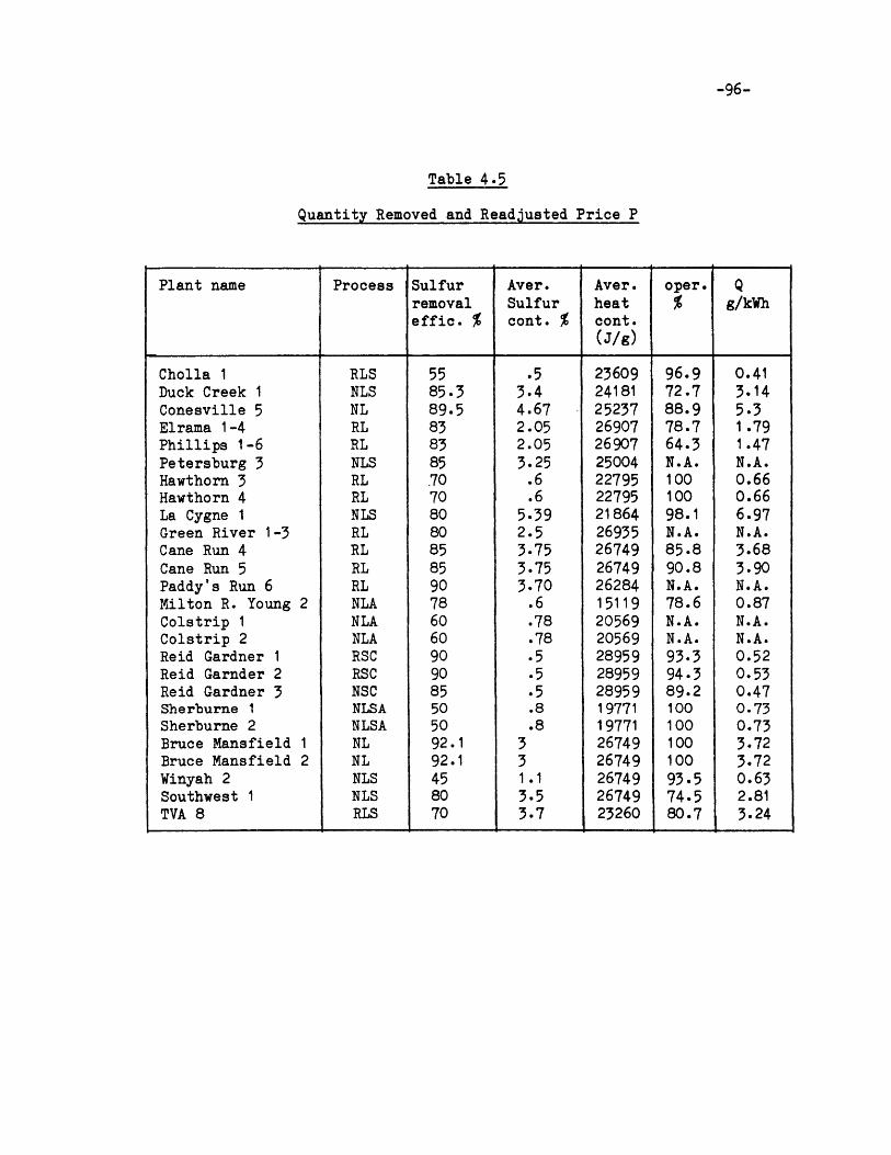
-96-
Table 4.5
Quantity Removed and Readjusted Price P
Plant name Process Sulfur Aver. Aver. oper. Qremoval Sulfur heat % g/kWheffic. % cont. % cont.
(J/g)
Cholla 1 RLS 55 .5 23609 96.9 0.41Duck Creek 1 NLS 85.3 3.4 24181 72.7 3.14Conesville 5 NL 89.5 4.67 25237 88.9 5.3Elrama 1-4 RL 83 2.05 26907 78.7 1.79Phillips 1-6 RL 83 2.05 26907 64.3 1.47Petersburg 3 NLS 85 3.25 25004 N.A. N.A.Hawthorn 3 RL 70 .6 22795 100 0.66Hawthorn 4 RL 70 .6 22795 100 0.66La Cygne 1 NLS 80 5.39 21864 98.1 6.97Green River 1-3 RL 80 2.5 26935 N.A. N.A.Cane Run 4 RL 85 3.75 26749 85.8 3.68Cane Run 5 RL 85 3.75 26749 90.8 3.90Paddy's Run 6 RL 90 3.70 26284 N.A. N.A.Milton R. Young 2 NLA 78 .6 15119 78.6 0.87Colstrip 1 NLA 60 .78 20569 N.A. N.A.Colstrip 2 NLA 60 .78 20569 N.A. N.A.Reid Gardner 1 RSC 90 .5 28959 93.3 0.52Reid Garnder 2 RSC 90 .5 28959 94.3 0.53Reid Gardner 3 NSC 85 .5 28959 89.2 0.47Sherburne 1 NLSA 50 .8 19771 100 0.73Sherburne 2 NLSA 50 .8 19771 100 0.73Bruce Mansfield 1 NL 92.1 3 26749 100 3.72Bruce Mansfield 2 NL 92.1 3 26749 100 3.72Winyah 2 NLS 45 1.1 26749 93.5 0.63Southwest 1 NLS 80 3.5 26749 74.5 2.81TVA 8 RLS 70 3.7 23260 80.7 3.24
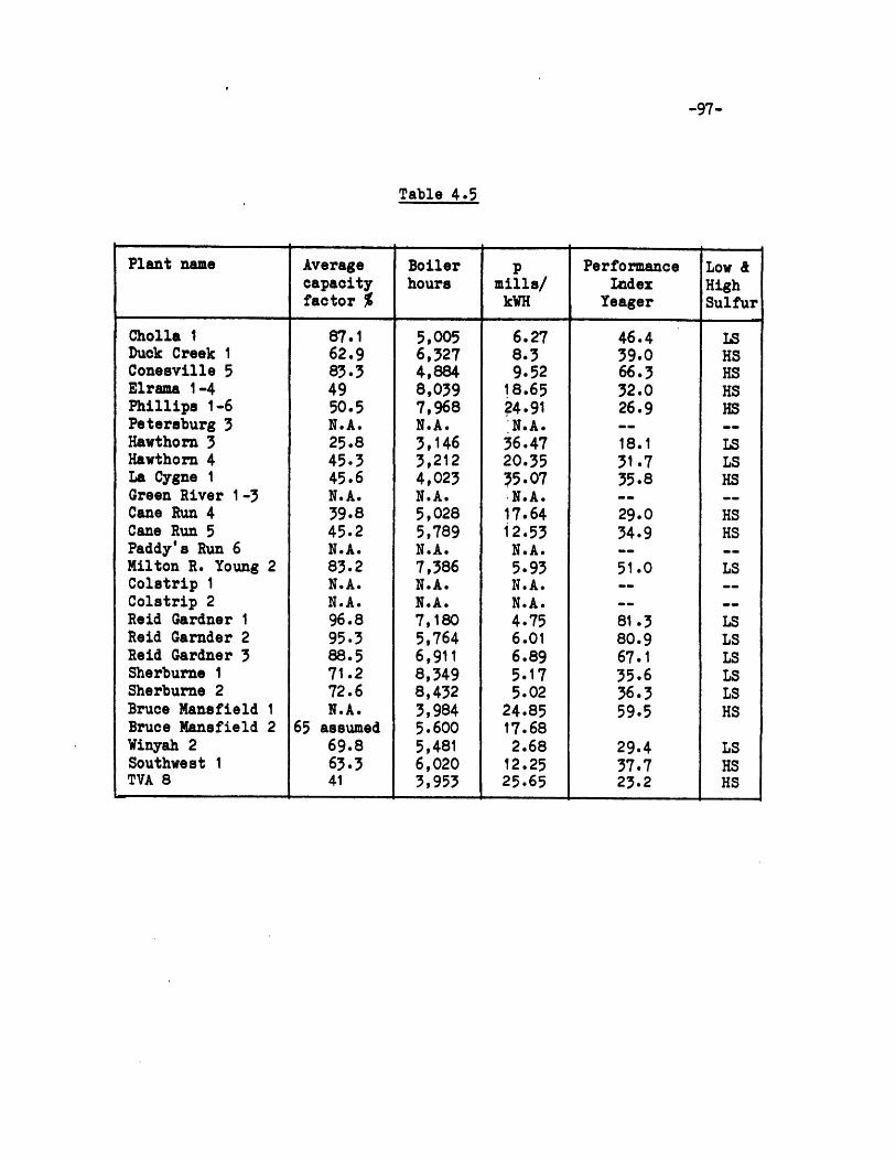
-97-
Table 4.5
Plant name Average Boiler p Performance Low &capacity hours mills/ Index Highfactor % kWH Yeager Sulfur
Cholla 1 87.1 5,005 6.27 46.4 LSDuck Creek 1 62.9 6,327 8.3 39.0 HSConesville 5 83.3 4,884 9.52 66.3 HSElrama 1-4 49 8,039 18.65 32.0 HSPhillips 1-6 50.5 7,968 24.91 26.9 HSPetersburg 3 N.A. N.A. -N.A. -- --Hawthorn 3 25.8 3,146 36.47 18.1 LSHawthorn 4 45.3 3,212 20.35 31.7 LSLa Cygne 1 45.6 4,023 5.07 35,8 HSGreen River 1-3 N.A. N.A. :N.A. -- --Cane Run 4 39.8 5,028 17.64 29.0 HSCane Run 5 45.2 5,789 12.53 34.9 HSPaddy's Run 6 N.A. N.A. N.A. -- --Milton R. Young 2 83.2 7,386 5.93 51.0 LSColstrip I N.A. N.A. N.A. -- --Colatrip 2 N.A. N.A. N.A. -- --Reid Gardner 1 96.8 7,180 4.75 81.3 LSReid Garnder 2 95.3 5,764 6.01 80.9 LSReid Gardner 3 88.5 6,911 6.89 67.1 LSSherburne 1 71.2 8,349 5.17 35.6 LSSherburne 2 72.6 8,432 5.02 36.3 LSBruce Mansfield 1 N.A. 3,984 24.85 59.5 HSBruce Mansfield 2 65 assumed 5.600 17.68Winyah 2 69.8 5,481 2.68 29.4 LSSouthwest 1 63.3 6,020 12.25 37.7 HSTVA 8 41 3,953 25.65 23.2 HS
011111
-98-
by economies of scale. This economic principle, however, does not seem to
be valid for the lime process, probably because the price of lime is four
times as much as the price of limestone.
The second observation can be interpreted as follows. For the same
price, the quantity of sulfur removed for new processes is greater than for
retrofit processes which means that the design of new scrubbers makes them
more efficient than the retrofit ones.
To obtain these data, different plants were looked at one point in
time, the year 1981. We assumed that these different firms were similar,
once the differences of capacity factor, operability and number of boiler
hours were removed. The principal difficulty is that the firms may not be
sufficiently similar and that the data collected may more correctly
represent "interutility" differences rather than reflecting a simple
relationship between quantity removed and costs. (Johnson, 1960)
Another method would have been to look at the quantity of sulfur
removed and cost data for a particular plant in different time periods.
(See Section 5) The difficulty with this method is that prices of inputs
may change over time. Such price changes will obviously affect costs
independently of how a utility's quantity of sulfur removed is changing.
(Nicholson, 1978)
The reason why this method was not used in this section is that many
data were missing for most of the utilities. Therefore I was not able to
derive these curves for all the plants of my survey. However, these curves
have been derived for the four utilities listed in the case studies in
Section 5.
It will be also noticed that the capital cost is not included in this
-"0 III MIhI I0Y1
-99-
annual cost, contrary to an usual average cost curve.
4.5 Conclusion
As the FGD technology moves along the learning curve, considerable
progress is made in resolving major problems that plague the initial FGD
installations. More work needs to be done, however, to optimize system
design and reduce cost and system energy demand without impairing
reliability and efficiency.
The design of the mist eliminators should be improved because of the
plugging of the lines due to precipitation of gypsum.
The instrumentation and process control strategies must be improved as
well as the construction materials used in FGD systems and related
equipment. The problem of corrosion is a very important one and reduces
the life of the scrubber and its components.
The study of the average cost curve shows a very big difference
between the adjusted cost P0 of 5.2 mills/kWh and a real cost P of 36.5
mills/kWh, which represents about 60% of the price of a kWh! However for
sodium carbonate and dual alkali processes this difference is smaller (P is
even smaller than PO).
Hence other methods of sulfur removal should be considered. The dry
collection processes should be investigated. A substantial amount of work
has already been done to verify process design using lime and sodium
carbonate reagents for low to medium sulfur coal applications. The
feasibility of dry collection for medium to high sulfur coal applications
-100-
could prove beneficial.
__________________________________________*IIIIIEIlHIIIYIELYY
-101-
5. CASE STUDIES
5.1 Introduction
In Section 3 and Section 4 we looked at a group of plants and we used
a statistical analysis to calculate the cost and to study the operation of
the FGD systems installed in the utilities.
In Section 5 we analyze the FGD systems as case studies. For each
category previously considered (New/Retrofit Limestone and New/Retrofit
Lime Scrubbing) one plant is selected. The criteria of selection are a
large unit capacity (125 MW), a good operability index (70%) and a good set
of data concerning the operation of the scrubber since its initial start
up.
Section 5.2.1, 5.3.1, 5.4.1, 5.5.1 contain descriptions and an
analysis of the evolution of the operability along the years for each of
the plants selected. The variations are explained and a comparison is
conducted between the FGD system and the category which it belongs to.
In Sections 5.2.2, 5.3.2, 5.4.2, 5.5.2 the evolution of costs is
described. Actually it would be more accurate to say that we consider the
evolution of the annual cost per kWh produced, since the capacity factor of
the plant and the number of boiler hours are the variables which determine
the cost. The average cost curves for each plant are drawn, using the
evolution of cost and operability previously studied.
Section 5.2.3, 5.3.3, 5.4.3, 5.5.3 summarize the problems encountered
in the case study.
Finally in Section 5.6 a comparison between the FGD system and the
category which it belongs to is performed. An attempt is made to explain
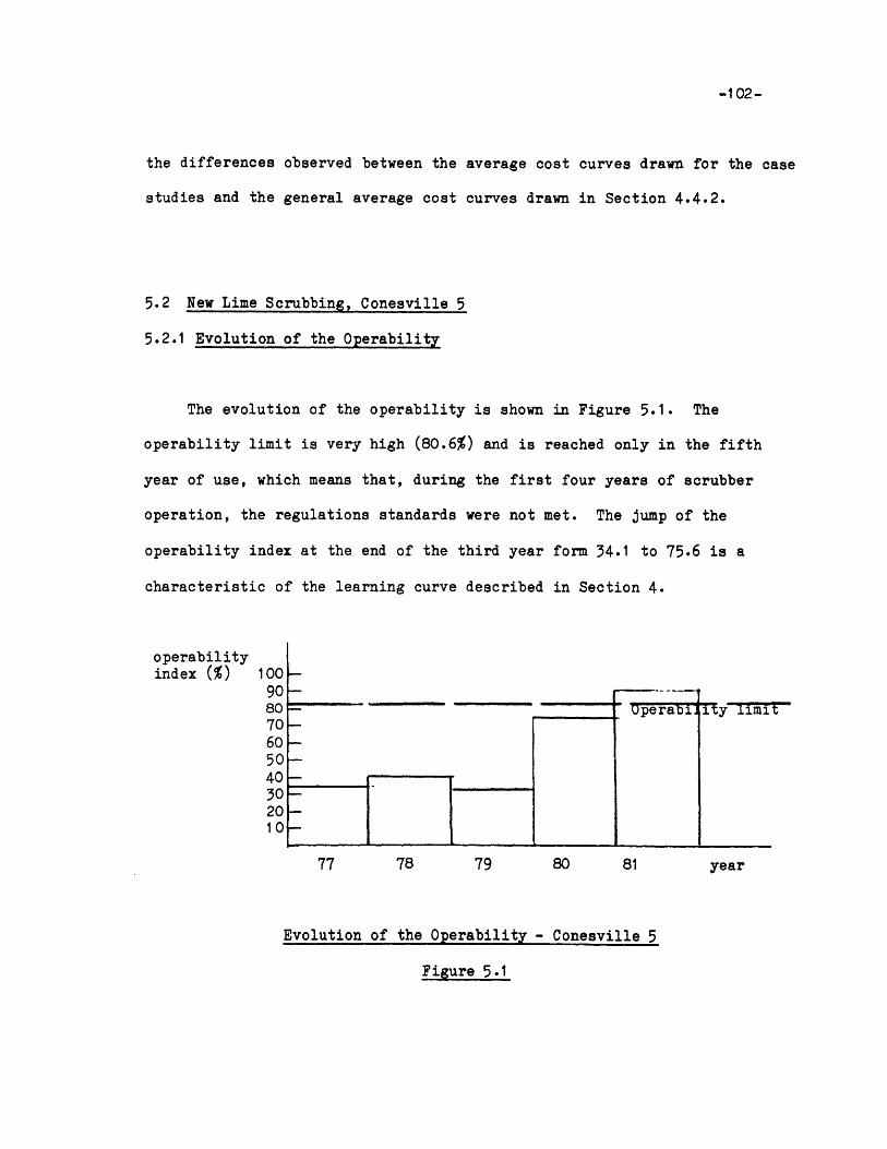
-102-
the differences observed between the average cost curves drawn for the case
studies and the general average cost curves drawn in Section 4.4.2.
5.2 New Lime Scrubbing, Conesville 5
5.2.1 Evolution of the Operability
The evolution of the operability is shown in Figure 5.1. The
operability limit is very high (80.6%) and is reached only in the fifth
year of use, which means that, during the first four years of scrubber
operation, the regulations standards were not met. The jump of the
operability index at the end of the third year form 34.1 to 75.6 is a
characteristic of the learning curve described in Section 4.
operabilityindex ( 100
908070605040302010
77 78 79 80 81 year
Evolution of the Operability - Conesville 5
Figure 5.1
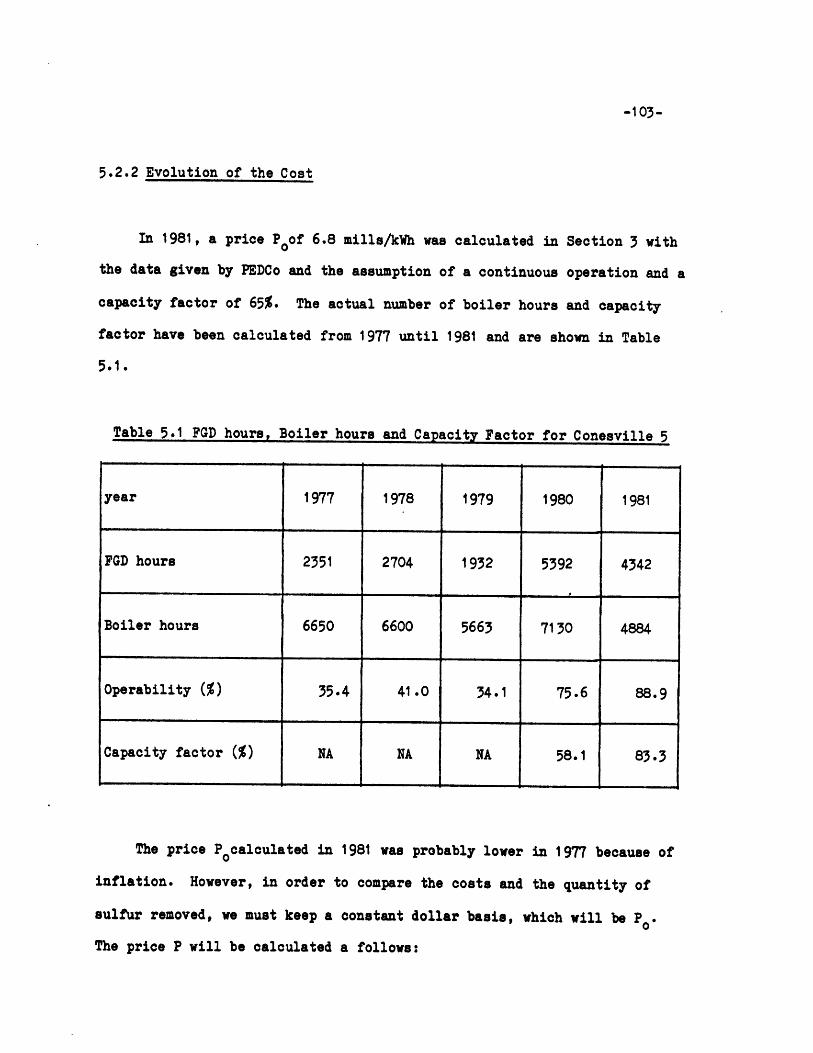
-103-
5.2.2 Evolution of the Cost
In 1981, a price P of 6.8 mills/kWh was calculated in Section 3 with
the data given by PEDCo and the assumption of a continuous operation and a
capacity factor of 65%. The actual number of boiler hours and capacity
factor have been calculated from 1977 until 1981 and are shown in Table
5.1.
Table 5.1 FGD hours, Boiler hours and Capacity Factor for Conesville 5
year 1977 1978 1979 1980 1981
FGD hours 2351 2704 1932 5392 4342
Boiler hours 6650 6600 5663 7130 4884
Operability (%) 35.4 41.0 34.1 75.6 88.9
Capacity factor (%) NA NA NA 58.1 83.3
The price Pocalculated in 1981 was probably lower in 1977 because of
inflation. However, in order to compare the costs and the quantity of
sulfur removed, we must keep a constant dollar basis, which will be Po.
The price P will be calculated a follows:
-e - ----- '~ 00111110IYIY MINI I, l1hI INIIIIIY YA WIIN IN

-104-
Po x 8760 x 0.65Boiler hours x Capacity factor
When the capacity factor is not available, the usual 65% capacity factor is
assumed.
The quantity Q of sulfur removed was calculated with the equation gien
in Section 4. The results are shown below in Table 5.2.
Table 5.2
Annual Cost and Quantity of Sulfur Removes
These results are drawn in Figure 5.5. The average cost curve obtained is
very flat, which means that the price is almost constant, whatever the
quantity of sulfur removed is.
5.2.3 Problems Encountered
After a fire which delayed the unit start up for one month, the early
operations began in January 1977 and were marked by cold weather and
year 1977 1978 1979 1980 1981
mills/kWh P 8.96 9.03 10.52 9.35 9.52
g/kWh Q 2.1 2.4 2.0 4.5 5.3
P =
-105-
related problems such as frozen lines. In April 1977, some plugging
occurred in the tube thickeners. Rocks up to five inches in diameter were
detected. It was decided to install mechanical separators and metal
detectors at the lime shipment facility. Many modifications and repairs
were made to the unit instrumentation system, to the absorber liner and to
the piping so that the FGD system was most often closed until the end of
1977. The operability for 1977 was 35.4%, which is well below the average
operability for the first year of operation, 57.6% calculated in Section 4.
We will also notice that the first year operability for the new lime
scrubbing category is 72.0%!
In 1978, the operability remained about the same for the same reasons.
In April 1978, the FGD system was down due to an excess of flocculant in
the thickener. This excess yielded a high solids level in the overflow and
resulted in plugging problems in the absorber modules. Finally, in May,
the thickener was emptied in order to restore a proper flocculant balance.
In July and August outage time was due to plugging in the mist eliminator.
In 1979, the operability index was the lowest since the start up.
During January and February, the scrubber did not work because of severe
winter weather. In March and April, module B did not operate because of
severe corrosion at the inlet presaturator duct. In May and June, the pH
lines were plugged. During the first three years of "operation", the FGD
system experienced all the problems listed in Section 4.
The problems encountered in 1980 were minor problems and therefore the
operability finally increased. The instrumentation and mist eliminator
nozzle plugging caused some FGD system outage time.
In 1981, the operability was above the operability limit. The FGD
- - YIIIIYIYIIIIYIII Y IIIIIIIYIIIIYYIYIIIYYIIIYI llliil-- 11 111-, , 11W 11-1 I, 111 W UM ON ON
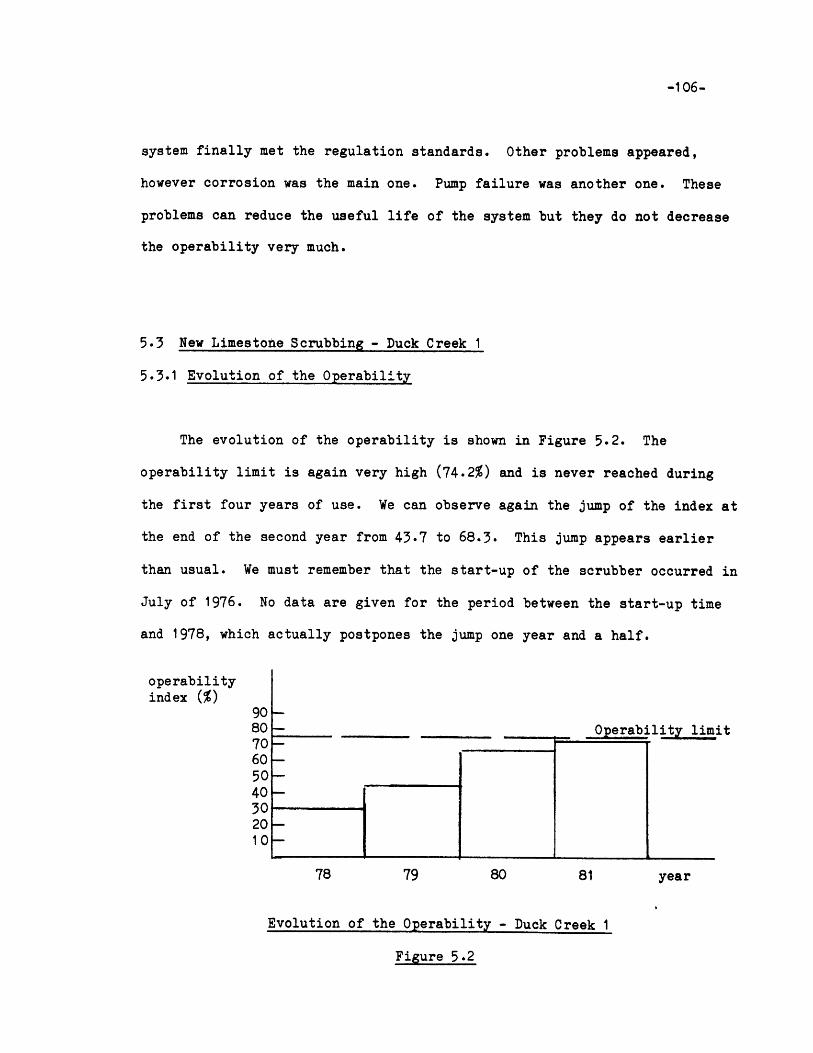
-106-
system finally met the regulation standards. Other problems appeared,
however corrosion was the main one. Pump failure was another one. These
problems can reduce the useful life of the system but they do not decrease
the operability very much.
5.3 New Limestone Scrubbing - Duck Creek 1
5.3.1 Evolution of the Operability
The evolution of the operability is shown in Figure 5.2. The
operability limit is again very high (74.2%) and is never reached during
the first four years of use. We can observe again the jump of the index at
the end of the second year from 43.7 to 68.3. This jump appears earlier
than usual. We must remember that the start-up of the scrubber occurred in
July of 1976. No data are given for the period between the start-up time
and 1978, which actually postpones the jump one year and a half.
operabilityindex (%)
9080 -- Operability limit70-605040 -302010
78 79 80 81 year
Evolution of the Operability - Duck Creek 1
Figure 5.2
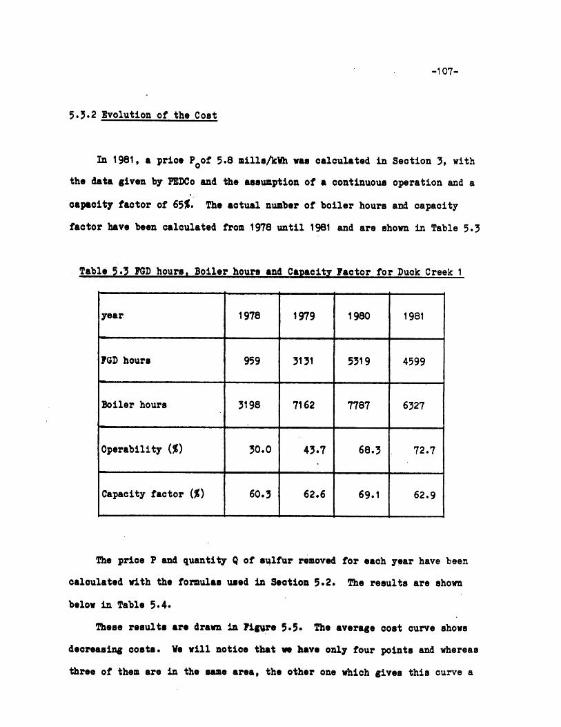
-107-
5.3.2 Evolution of the Cost
In 1981, a price Poof 5.8 mills/kWh was calculated in Section 3, with
the data given by PEDCo and the assumption of a continuous operation and a
capacity factor of 65%. The actual number of boiler hours and capacity
factor have been calculated from 1978 until 1981 and are shown in Table 5.3
Table 5.3 POD hours, Boiler hours and Capacity Factor for Duck Creek 1
year. 1978 1979 1980 1981
FGD hours 959 3131 5319 4599
Boiler hours 3198 7162 7787 6327
Operability (%) 30.0 43.7 68.3 72.7
Capacity factor (0) 60.3 62.6 69.1 62.9
The price P and quantity Q of sulfur removed for each year have been
calculated with the formulas used in Section 5.2. The results are shown
below in Table 5.4.
These results are drawn in Figure 5.5. The average cost curve shows
decreasing costs. We will notice that we have only four points and whereas
three of them are in the same area, the other one which gives this curve a
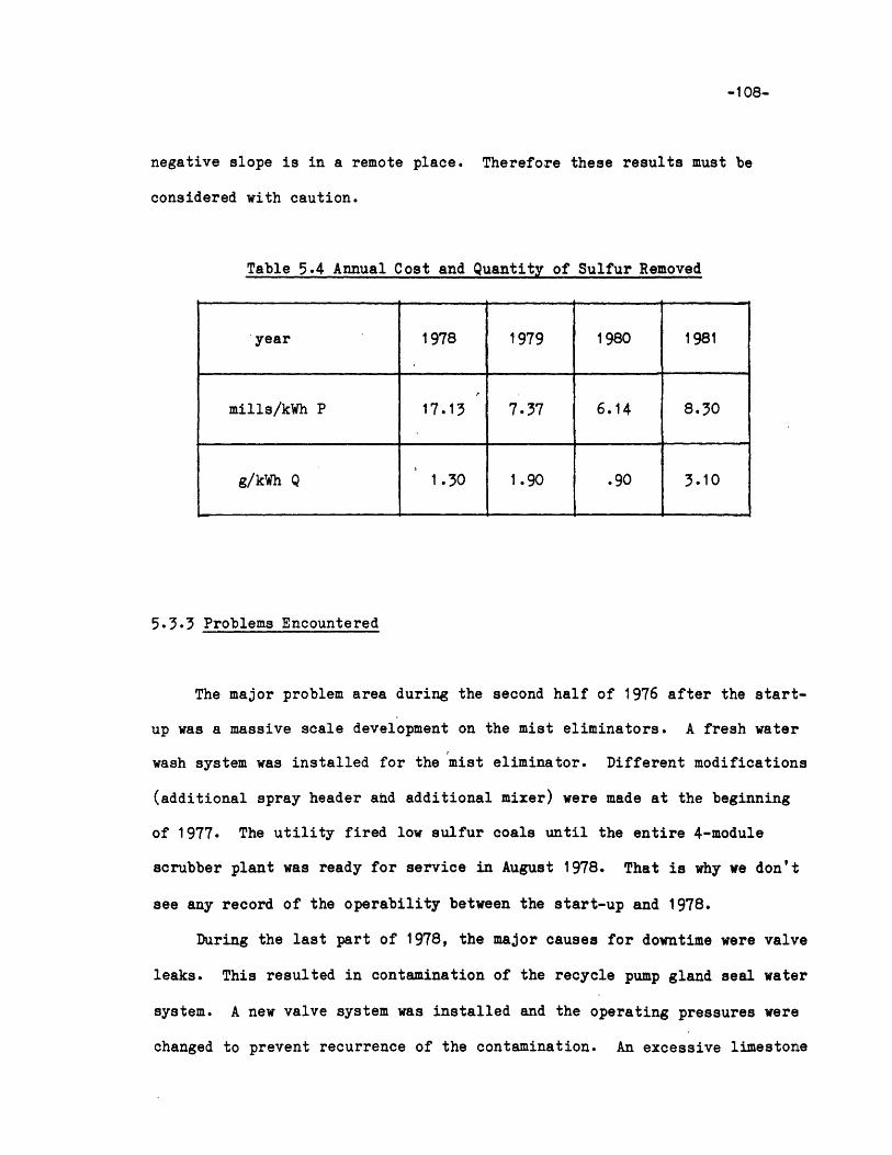
-108-
negative slope is in a remote place. Therefore these results must be
considered with caution.
Table 5.4 Annual Cost and Quantity of Sulfur Removed
year 1978 1979 1980 1981
mills/kWh P 17.13 7.37 6.14 8.30
g/kWh Q 1.30 1.90 .90 3.10
5.3.3 Problems Encountered
The major problem area during the second half of 1976 after the start-
up was a massive scale development on the mist eliminators. A fresh water
wash system was installed for the mist eliminator. Different modifications
(additional spray header and additional mixer) were made at the beginning
of 1977. The utility fired low sulfur coals until the entire 4-module
scrubber plant was ready for service in August 1978. That is why we don't
see any record of the operability between the start-up and 1978.
During the last part of 1978, the major causes for downtime were valve
leaks. This resulted in contamination of the recycle pump gland seal water
system. A new valve system was installed and the operating pressures were
changed to prevent recurrence of the contamination. An excessive limestone
-109-
carryover to the mist eliminator was also noted. The top rod deck was
removed to improve gas flow and eliminate the carryover problem.
In the early months of 1979, frosen line problems were experienced.
Freezing problems continued to hamper GD operations during March. In the
last three quarters of the year two major problems were encountered: the
mist eliminator was plugged (already a start-up problem three years ago)
and storage pump leaks were reported as well as recycle pump failures.
In 1980, the operability almost reached 70%, still below the
operability limit. The main problems encountered are due to leaks and
repairs because of aging materials. Among replacements were the replacement
of the limestone storage tank mixer motor and of the ball mill motor.
The operability reached its maximnu in 1981 at 72.7%. However the
major problem of Duck Creek 1, plugging, is not yet solved. This is the
main reason why the operability did not reach 100%. Extensive plugging was
observed at the beginning of April, resulting in the need for extensive
maintenance, cleaning, repairs, and upgrading of each module.
Clearly, at the end of 1981, the plugging problem remained at Duck
Creek 1. This problem caused outage time which resulted in a low
availability of the system and consequently a quicker deterioration of the
main parts of the equipment (lines, pup, fana,...).
5.4 Retrofit Lime Scrubbing - Cane Run 4
5.4.1 Evolution of the Operability
Whereas the two former case studies, Conesville 5 and Duck Creek 1,
I I
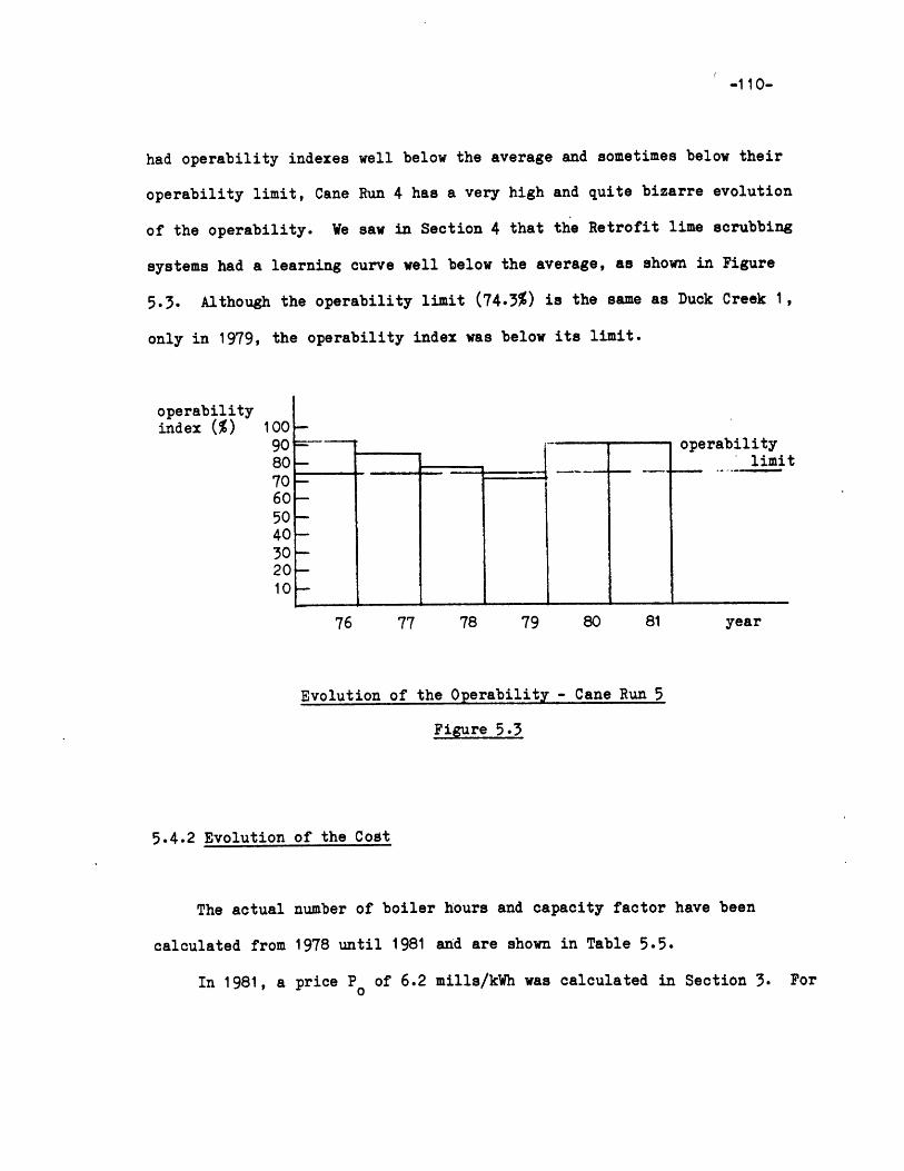
-110-
had operability indexes well below the average and sometimes below their
operability limit, Cane Run 4 has a very high and quite bizarre evolution
of the operability. We saw in Section 4 that the Retrofit lime scrubbing
systems had a learning curve well below the average, as shown in Figure
5.3. Although the operability limit (74.3%) is the same as Duck Creek 1,
only in 1979, the operability index was below its limit.
operabilityindex (%) 100
90 - - operability80 -- limit
70 --60 --
50 -4030 --
76 77 78 79 80 81 year
Evolution of the Operability -
Figure 5.3
Cane Run 5
5.4.2 Evolution of the Cost
The actual number of boiler hours and capacity factor have been
calculated from 1978 until 1981 and are shown in Table 5.5.
In 1981, a price Po of 6.2 mills/kWh was calculated in Section 3. For
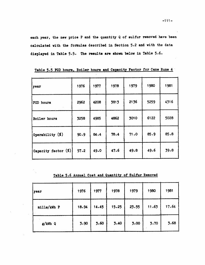
-111-
each year, the new price P and the quantity Q of sulfur removed have been
calculated with the formulas described in Section 5.2 and with the data
displayed in Table 5.5. The results are shown below in Table 5.6.
Table 5.5 FGD hours, Boiler hours and Capacity Factor for Cane Rune 4
year 1976 1977 1978 1979 1980 1981
FGD hours 2962 4208 3813 2136 5259 4316
Boiler hours 3258 4985 4862 3010 6122 5028
Operability (%) 90.9 84.4 78.4 71.0 85.9 85.8
Capacity factor (%) 57.2 49.0 47.6 49.8 49.6 39.8
Table 5.6 Annual Cost and Quantity of Sulfur Removed
-112-
The results are drawn in Figure 5.5. The average cost curve is very
inelastic. The price varies a lot whereas the quantity of sulfur removed
remains about the same. This high inelasticity is due to the evolution of
the operability which is almost constant. Actually this average cost curve
represents the product of the number of boiler hours times the capacity
factor versus the operability, since the reference price P, remains
constant as well as the scrubber design removal efficiency, the coal heat
content and the coal sulfur content.
5.4.3 Problems Encountered
The problems are quite different from the problems encountered during
the two previous case studies because of the high level of operability. In
1976, there were some minor problems with the spray nozzles in the mobile
bed contactor. The plastic expanded due to the high operating temperatures
and blocked the slurry feed. These nozzles were replaced with ceramic
constructed components.
At the beginning of 1977, the FGD system was taking off line, as
usual, because of the freezing problem. The reason for Cane Run 4 is
linked to the supply of Lime which ceased because the barges could not come
due to the Ohio River freeze up. No real problem was encountered later on.
A few modifications were completed. For instance, a new spray header was
added to increase the liquid gas ratio. In September 1977 the FGD system
was officially proved to have achieved compliance.
In 1978, the operability index decreased from 84.4% to 78.4%, mainly

-113-
because of severe winter weather.
The scrubber was off line during the month of September 1979, due to a
mechanical failure with the damper gates. This is the reason why the
operability index is the lowest (71.0%).
In 1980, the operability increased again due to mild winter weather,
in spite of several failures which occurred during the last months of 1980.
Different failures (spray pump, valves, ductwork and mist eliminators)
caused some outage time. This is part of the maintenance necessary to
repair a material which becomes old.
No major problems were encountered during 1981. However, in August
1981 the traditional FGD problem, plugging, appeared in the absorber module
and caused some outage time.
This FGD system is very unusual. The learning curve does not appear
and thus no major problems wer encountered. The only reason why the
operability does not reach 100% is a problem of lime supply during the
winter. How can it be solved? Papermills which receive wqod through the
rivers begin stocking a bigger pile of wood during the summer and the fall
in order not to be stopped because of the river freeze up. Cane Run 4 has
problably already considered this eventuality but the investment necessary
to overstock the lime might be too high. Another solution would be to buy
lime from another producer during the winter. Once again, the problem can
be solved but the real question is: Is it worth spending extra money just
to decrease sulfur emissions since the EPA has officially approved the
scrubber?

-114-
5.5 Retrofit Limestone Scrubbing - Cholla 1
5.5.1 Evolution of the Operability
The operability limit for Cholla 1 is 0. Therefore a low operability
index is expected. These expectations are different from reality. A
traditional learning curve is observed with an early jump at the end of the
first year from 65.1% to 84.7%. Although the data for 1981 were not
available, seven years (74-80) of data have been recorded and the 1980
operability index is 96.9%.
operability operabilityindex (%) 100- . limit - 0
90 -80 -70-60 -
74 75 76 77 78 79 80 year
Evolution of the Operability - Cholla 1
Figure 5.4
5.5.2 Evolution of the Cost
The actual number of boiler hours and capacity factor have been
calculated from 1974 until 1980 and are shown in Table 5.7.
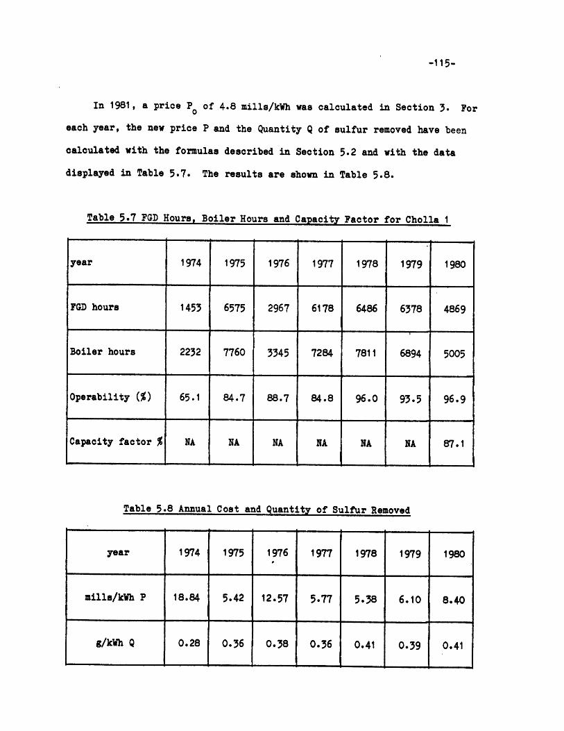
-115-
In 1981, a price Po of 4.8 mills/kWh was calculated in Section 3. For
each year, the new price P and the Quantity Q of sulfur removed have been
calculated with the formulas described in Section 5.2 and with the data
displayed in Table 5.7. The results are shown in Table 5.8.
Table 5.7 FGD Hours, Boiler Hours and Capacity Factor for Cholla 1
year 1974 1975 1976 1977 1978 1979 1980
FGD hours 1453 6575 2967 6178 6486 6378 4869
Boiler hours 2232 7760 3345 7284 7811 6894 5005
Operability (%) 65.1 84.7 88.7 84.8 96.0 93.5 96.9
Capacity factor % NA NA NA NA NA NA 87.1
Table 5.8 Annual Cost and Quantity of Sulfur Removed
year 1974 1975 1976 1977 1978 1979 1980
mills/kWh P 18.84 5.42 12.57 5.77 5.38 6.10 8.40
g/kWh Q 0.28 0.36 0.38 0.36 0.41 0.39 0.41

-116-
P (Mil.s/kh)
24
Cane Run 4 (L)
+ RL
NLS
ars
Cholla
VRLS)SRLS
Duck Creek 1 +(NLS)
1 + $L
+ NIL +bonesville 5N + NLS (NL)
+ NLS
* RLS9 RLS9 RLS
Q(g/kWh)1 2 3 4 5 6
Case Studies - Average Cost Curves
Figure 5.5
21
18.-
15-
12-
9+
3+
0 ~
RLS RL
%
+ N
-117-
The results are drawn in Figure 5.5. The average cost curve is
similar to the Cane Run 4 case. Since the operability is very high and
almost constant, the quantity of sulfur removed remains constant whereas
the price varies following the number of boiler hour fluctuations. The
quantity of sulfur removed per kWh is very small. This is due to the low
sulfur content of the coal used by Cholla 1 and a consequence of the zero
operability limit.
5.5.3 Problems Encountered
The main problem which occurred after the commercial startup in
December 1973 was a vibration problem. The difference in the size of the
main duct and reheated transition duct caused the gas flow to produce
harmonic vibrations in the reheater. The installation of baffles partially
dampened the vibrations.
The two other problems which appeared are classical FGD problems:
corrosion and plugging. One of the reheater bundles was badly corroded by
acid that condensed in the uninsulated duct upstream of the reheaters. The
tube bundle was replaced, a baffle was installed to divert condensed acid
from reheater tubes and the duct upstream of the reheater was insulated.
When the system operated at low flow rates, some lines plugged, solids
settled out in standby pumps and excessive fan vibrations occurred because
of an accumulation of scale buildup when the unit was idle. To solve these
problems the piping was modified to eliminate stagnant pockets, the pumps
were flushed immediately after removal from service and the fan was
'~---...-'-~-~ -- - - - ~- _.- F-_C __~__ _L=__ ___
-118-
sandblasted.
Operation of the system throughout 1975 and 1976 was accompanied by a
number of minor problem areas related to plugging and corrosion. the
operability was very high during these two years at about 85%. As a
consequence of the corrosion/erosion problem, many leaks were discovered at
sensitive points of the scrubber. The last 15% necessary to reach 100%
were due to intensive repairs and maintenance caused by these multiple
minor problems. The weather in the winter did not seem to be a problem.
During 1977, routine maintenance was required. In December, the
overhaul period began. Therefore the boiler and scrubbing system were out
of service. Evidence of chloride attack was found in the liquid gas
centrifugal separator shell and on the reheater tubes. Extensive corrosion
was also discovered in the ductwork. Although the utility had recoated
different parts, the problem was not fully resolved.
During 1978, 1979, and 1980, no major problems were reported. A very
high operability index (around 95%) means that the only outage time was due
to routine maintenance.
It is amazing to see how busy people can be trying to improve the
operability level when they know that the operability limit is zero and
that the scrubber is not necessary. Usually utilities with a zero
operability limit have a very high operability index. An explanation could
be the following: the utilities which have a zero operability limit have
not much sulfur to remove from their coal. Therefore the usual plugging
and corrosion problems have not the same gravity as for a utility with a
high operability limit.
-119-
5.6. Conclusion
The comparison of the average cost curves obtained for each of these
case studies with the curves obtained in Section 4 for the corresponding
category is interesting. Striking differences can be observed and
explained by the two following considerations.
As we saw in this section, each case study is not really a good
representative of the category which it belongs to. Therefore the average
cost curves drawn in Figure 5.5 give only a partial view of what the real
curves look like.
We must also consider the fact that the curves drawn in Figure 5.5.
are drawn with data given for a period ranging from 4 to 7 years, whereas
the curves drawn in Figure 4.8 are drawn for the year 1981 only. Therefore
these later curves can be viewed as short run curves, while the former ones
can be viewed as long run curves, which are the aggregate of different
short run curves.
_ I III' L_ - .:~IIIIPI~-
-120-
6 CONCLUSIONS AND RECOMMENDATIONS
6.1 Conclusions
The cost analysis shows that the limestone wet scrubbing process is
the cheapest of all FGD processes. It is also cheaper to install a
scrubber on a plant which uses low-sulfur coal than on a plant which uses
high-sulfur coal. The financial analysis which takes into account capital
and annual costs reduces the gap between retrofit and new scrubbers. The
overall result is that scrubbing raises utility capital requirements by 25
percent and electricity bills by at least 15 percent if we assume that the
burden of the FGD technology is totally shifted onto the consumer.
Our functional analysis shows that the scrubber becomes operational
only three years after the start-up date, which corresponds to a move along
the learning curve. However the scrubber works well when it removes almost e
no sulfur (low-sulfur coal) whereas problems of plugging and corrosion
prevent a good performance of the scrubber which "tries" to remove a lot of
sulfur (high-sulfur coal).
Moreover the operability limit defined as the minimum operability
necessary to meet the regulations is too high for high-sulfur coals, and in
most cases even after five or more years the regulations are still not met.
On the other hand, scrubbers controlling the emissions from plants burning
low-sulfur coal have a zero operability limit, which means that the
regulations are met even without scrubbers. It is a result of the New
Source Performance Standards which require every new plant to install a
scrubber. Ironically, these low-sulfur scrubbers do not have many
problems. This is logical since they do not remove much sulfur.
-121-
6.2 Recommendations
Therefore the legislation should be changed. A mandate such as "All
new plants must install scrubbers" must be avoided and replaced by the
"Best available Technology" introduced in the Clean Air Act of 1970. For
existing scrubbers, the operability limit should be the same, whatever the
location or the type of coal used. It means that the standards should
become more stringent for low-sulfur coals (in order to increase the
operability limit) and less stringent for high-sulfur coals (in order to
reduce the operability limit). However we know from the past that the
solution chosen differs from the rational solution. In this particular
problem a consensus must be found between the different stakeholders who
are the environmentalists, the utilities, the Department of Energy, the
coal miners and the FGD system designers.
In addition to its economic, energy and environmental impacts, the
United States' decision on whether and how to implement control strategies
could have international implications. At a November 1980 conference on
acid precipitation in Portland, Maine, the Parliamentary Secretary of the
Canadian Ministry of the Environment made his government's position clear:
"The official position of the government of Canadais that we cannot wait for a perfect understandingof the acid precipitation phenomenon before movingto control it."
However the legislator cannot be blamed for the poor performance of
the scrubber. Research and Development must be pursued in order to optimize
system design and reduce cost and system energy demand. Improvement of
-122-
mist elimination and instrumentation as well as optimization of
construction materials will reduce the plugging and corrosion problems.
Investigation of other processes like dry collection should be
conducted. A substantial amount of work has already been made to verify
process design using lime and sodium carbonate reagents for low to medium
sulfur coal applications. The feasibility of dry collection for medium to
high sulfur coal applications could prove beneficial and shoud be
investigated. Also R&D on "in-combustion" sulfur removal, (e.g. lime
injected multistage burner (LIMB) should be further increased.
Finally a constant enforcement pressure might improve the operability!
Today, inspection visits are few and far between. The regulators rely on
the polluters themselves to supply data on their scrubbing efficiency and
thus regulators are unable to distinguish reliable from unreliable
information. Unqualified utility employees are sent to the scrubbing
operation. We know that scrubbers constantly demand creative tending when
they become clogged or corroded. Therefore a conscientious and highly
competent staff is an absolute requirement. Why, for instance, is there
such a difference between the Japanese and American operability of
scrubbers? People believe that the successful use of scrubbers in Japan is
due to the strength of the Japanese enforcement program. The Japanese
operate control research centers that are usually linked directly, via
telemetry, to stations monitoring emissions from a major source.
It is therefore important for the EPA to create an administrative
infrastructure equal to the challenge of enforcement.
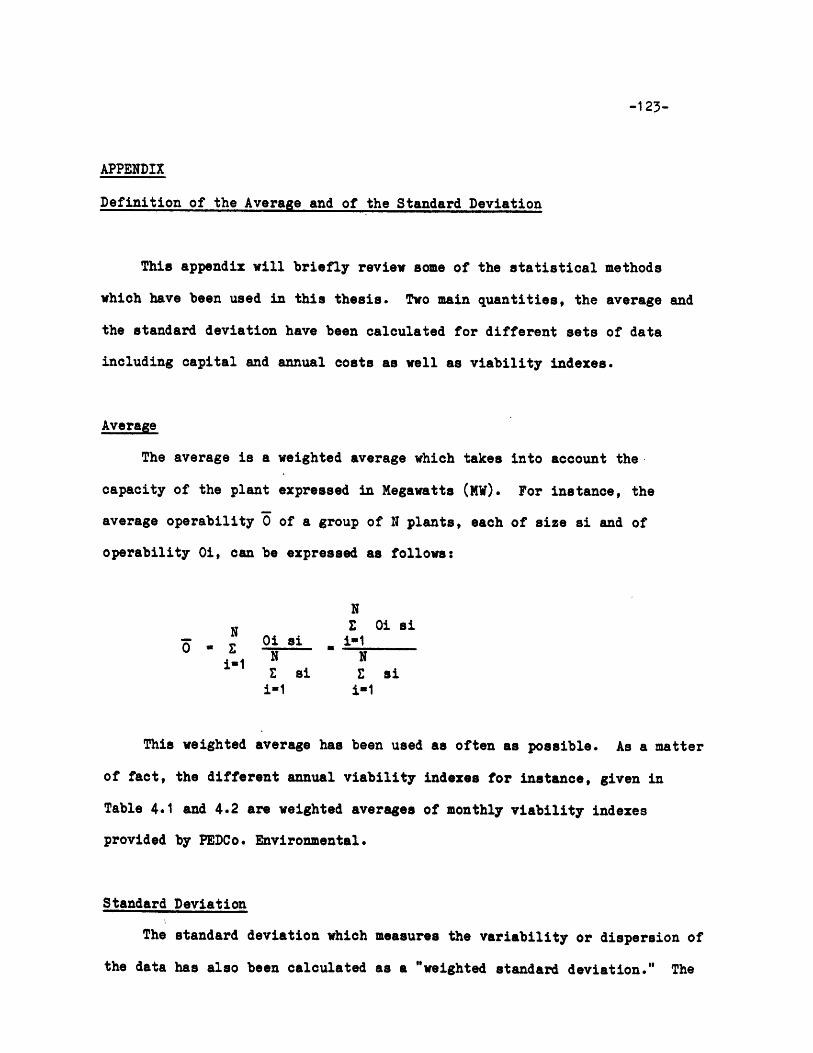
-123-
APPENDIX
Definition of the Average and of the Standard Deviation
This appendix will briefly review some of the statistical methods
which have been used in this thesis. Two main quantities, the average and
the standard deviation have been calculated for different sets of data
including capital and annual costs as well as viability indexes.
Average
The average is a weighted average which takes into account the
capacity of the plant expressed in Megawatts (MW). For instance, the
average operability 0 of a group of N plants, each of size si and of
operability Oi, can be expressed as follows:
NN E Oi si
Oisi i-i0 E 0-
N NE si E sii=1 i-1
This weighted average has been used as often as possible. As a matter
of fact, the different annual viability indexes for instance, given in
Table 4.1 and 4.2 are weighted averages of monthly viability indexes
provided by PEDCo. Environmental.
Standard Deviation
The standard deviation which measures the variability or dispersion of
the data has also been calculated as a "weighted standard deviation." The
----;x------.~ __ ;; --~_.~ ?r - ~im .;-r+----- I _---
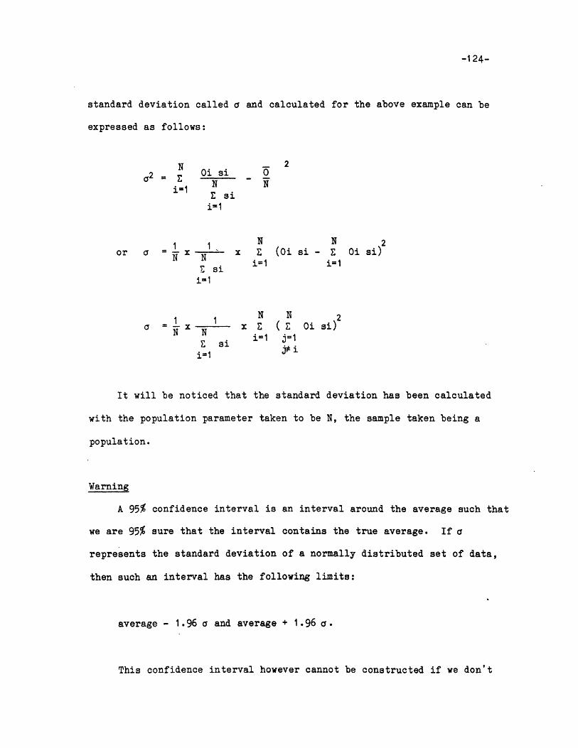
-124-
standard deviation called a and calculated for the above example can be
expressed as follows:
N 22 Oi si 0
N Ni=1z sii=1
o x N N 2
i= 1or a X I x E (Oi si - E
N NN 2
a X N x z (z Oisi)i=1 j=1
i=1
It will be noticed that the standard deviation has been calculated
with the population parameter taken to be N, the sample taken being a
population.
Warning
A 95% confidence interval is an interval around the average such that
we are 95% sure that the interval contains the true average. If a
represents the standard deviation of a normally distributed set of data,
then such an interval has the following limits:
average - 1.96 a and average + 1.96 a.
This confidence interval however cannot be constructed if we don't
-125-
have a normal distribution. Another analysis should be done to construct
such intervals in case for instance of exponential or t-distributions.
The standard deviation can always be calculated and measure the
variability or the dispersion of the data (it is called risk in finance).
However only in the case of a normal distribution can it be interpreted as
the boundary of a confidence interval.
-126-
REFERENCES r
Ackerman, B.A., and W.T. Hassler, 1981, Clean Coal/Dirty Air, Yale
University Press, New Haven, Connecticut.
Anderson, R.J., R.O. Reid, and E.P. Sesking, 1979, An Analysis of
Alternatives Policies for Attaining and Maintaining a Short Term NO,
Standard, Mathtech, Inc. Princeton, N.J.
Berman, I.M., 1981, "New generating capacity: when, where and by whom?"
Power Engineering, Vol. 85, No. 4, pp. 72-81.
Braley, R., and S. Myers, 1981, Principles of Corporate Finance, McGraw-
Hill Book Co., Inc., New York.
Bruck, N.G., and M.T. Melia, 1981, Design and Performance Data for
Operational FGD Systems EPA utility FGD survey Contract No. 68-02-
3173.
Bruck, N., M. Melia, R. McKibben, and B. Pelsori, 1982, Design and
Performance Data For Operational FGD Systems EPA utility FGD survey
April June 1982 Contract No. 68-02-3173.
Burchard, J.K., 1972, "Some general considerations of Flue Gas scrubbing
for utilities" in Proceedings-Sulphur and Utility Fuels: The Growing
Dilemma McGraw-Hill Book Co., Inc., New York, pp. 91-124.
Chapman, R.A., and M.A. Wells, 1981, Coal Resources and Sulphur Emission
Regulations Teknekron Inc., Report to EPA, EPA-600/7-81-086, Berkeley,
CA 94704.
Chem. Systems International Ltd., 1976, Reducing Pollution from Selected
Energy Transformation Sources, Graham and Trotman Ltd., London United
Kingdom.
-127-
Cowling, E., 1980, Acid Precipitaiton and Its Ecological Consequences, North
Carolina State University, Raleigh, N.C.
Curtis, C., 1980, Before The Rainbow: Wht We Know About Acid Rain, Edision
Electric Institute, Washington, D.C.
Devitt, T.W. and B.A. Laseke, 1980, "Utility Flue Gas Desulfurization in the
U.S." Chemical Engineering Progress, Vol. 76, No. 5, pp. 45-57.
Dumanoski, D., 1982, "Acid Politics" Technology Review, October 1982, pp.
64-66.
Haug, N., G. Oelert, and G. Weisser, 1979, Appendix 95-B-Lime/Sludge Flue
Gas Desulfurization Process, January, NTIS PB-295 003, Springfield,
Virginia.
Johnson, J., 1960, Statistical Cost Analysis, McGraw-Hill Book Co., Inc.,
New York, N.Y.
Kaplan, N., 1979, Summary of Utility Dual Alkali Systems, Industrial
Environment Research Laboratory Office of Research and Development,
U.S. EPA.
Kennedy, C., and A.P. Thirwal, 1972, "Surveys in Applied Economics:
technical progress" Economic Journal 82, No. 325, pp. 11-72.
Mansfield, E., 1980, Principles of Microeconomics, 3rd. edition, Norton New
York, N.Y.
Nicholson, W., 1978, Microeconomic Theory, The Dryden Press, Hinsdale,
Illinois.
Princiotta, F., R.W. Gerstle, and E. Schindler, 1979, Appendix 95-A-
Limestone/Sludge Flue Gas Desulfurization Process, January, NTIS PB-
295 002 Springfield, Virginia.
Silverman, B.C., 1982, "Acid Rain and a comparative analysis of two large-
-128-
scale electric utility models" Journal of Air Pollution Control t
Association, Vol. 32, No. 10, pp. 1031-1042.
Slack, A.V. and G.A. Hollinden, 1975, Sulfur Dioxide Removal from Waste
Gases, Noyes Data Corporation, Park Ridge, N.J.
U.S. EPA, Sulfur Oxid Control Technology Assessment Panel, 1973, Final
Report of the Sulfur Oxid Control Technology Assessment Panle to the
Federal Interagency Committee of Evaluation of State Air
Implementation Plans, Washington, D.C.
U.S. EPA, 1980, Acid Rain, EPA-600/9-79-036 p. 22.
U.S. EPA, 1980, Selected Impact of Electric Utility Operations in the Ohio
River Basin (1976-2000), Washington, D.C.
U.S. Department of Energy, 1980, Publ. No. DOE/EIA-0095, Energy Information
Adminstration Office of coal and electric power statistics.
Wilcox, C., and W.G. Sheperd, 1975, Public Policies Toward Business, 5th
edition Irwin Homewood, Illinois, pp. 391-422.
Yeager, K.E., 1978, Direct Use of Coal. Impact of Best Available Control
Technology, Proc. 5th energy techn. conf. Washington, D.C.
I