Fluctuations of eigenvalues and second order Poincaré inequalities

Probab. Theory Relat. Fields (2009) 143:1–40DOI 10.1007/s00440-007-0118-6

Fluctuations of eigenvalues and second order Poincaréinequalities

Sourav Chatterjee

Received: 16 May 2007 / Revised: 18 October 2007 / Published online: 30 November 2007© Springer-Verlag 2007

Abstract Linear statistics of eigenvalues in many familiar classes of randommatrices are known to obey gaussian central limit theorems. The proofs of such resultsare usually rather difficult, involving hard computations specific to the model in ques-tion. In this article we attempt to formulate a unified technique for deriving such resultsvia relatively soft arguments. In the process, we introduce a notion of ‘second orderPoincaré inequalities’: just as ordinary Poincaré inequalities give variance bounds,second order Poincaré inequalities give central limit theorems. The proof of the mainresult employs Stein’s method of normal approximation. A number of examples areworked out, some of which are new. One of the new results is a CLT for the spectrumof gaussian Toeplitz matrices.

Keywords Central limit theorem · Random matrices · Linear statistics of eigen-values · Poincaré inequality · Wigner matrix · Wishart matrix · Toeplitz matrix

Mathematics Subject Classification (2000) 60F05 · 15A52

1 Introduction

Suppose An is an n×n matrix with real or complex entries and eigenvalues λ1, . . . , λn ,repeated by multiplicities. A linear statistic of the eigenvalues of An is a function of the

The author’s research was partially supported by NSF grant DMS-0707054 and a Sloan ResearchFellowship.

S. Chatterjee (B)Department of Statistics, University of California at Berkeley,367 Evans Hall#3860, Berkeley, CA 94720-3860, USAe-mail: [email protected]: http://www.stat.berkeley.edu/∼sourav

123

2 S. Chatterjee

form∑n

i=1 f (λi ), where f is some fixed function. Central limit theorems for linearstatistics of eigenvalues of large dimensional random matrices have received consider-able attention in recent years. A very curious feature that makes these results unusualand interesting is that they usually do not require normalization, i.e., one does not haveto divide by

√n; only centering is enough. Moreover, they have important applications

in statistics and other applied areas (see e.g., the recent survey by Johnstone [35]).The literature around the topic is quite large. To the best of our knowledge, the

investigation of central limit theorems for linear statistics of eigenvalues of largedimensional random matrices began with the work of Jonsson [36] on Wishart matri-ces. The key idea is to express

∑λk

i as

∑λk

i = Tr(Akn) =

∑

i1,i2,...,ik

ai1i2 ai2i3 · · · aik−1ik aik i1 ,

where An is an n × n Wishart matrix, and then apply the method of moments to showthat this is gaussian in the large n limit. In fact, Jonsson proves the joint convergence ofthe law of (Tr(An),Tr(A2

n), . . . ,Tr(Apn )) to a multivariate normal distribution (where

p is fixed).A similar study for Wigner matrices was carried out by Sinaı̆ and Soshnikov [46,47].

A deep and difficult aspect of the Sinaı̆–Soshnikov results is that they get central limittheorems for Tr(Apn

n ), where pn is allowed to grow at the rate o(n2/3), instead ofremaining fixed. They also get CLTs for Tr( f (An)) for analytic f .

Incidentally, for gaussian Wigner matrices, the best available results are due toJohansson [34], who characterized a large (but not exhaustive) class of functions forwhich the CLT holds. In fact, Johansson proved a general result for linear statisticsof eigenvalues of random matrices whose entries have a joint density with respectto Lebesgue measure of the form Z−1

n exp(−n Tr V (A)), where V is a polynomialfunction and Zn is the normalizing constant. These models are widely studied in thephysics literature. Johansson’s proof relies on a delicate analysis of the joint densityof the eigenvalues, which is explicitly known for this class of matrices.

Another important contribution is the work of Diaconis and Evans [21], who provedsimilar results for random unitary matrices. Again, the basic approach relies on themethod of moments, but the computations require new ideas because of the lackof independence between the matrix entries. However, as shown in [20,21], strik-ingly exact computations are possible in this case by invoking some deep connectionsbetween symmetric function theory and the unitary group.

An alternative approach, based on Stieltjes transforms, has been developed in Baiand Yao [5] and Bai and Silverstein [6]. This approach has its roots in the semi-rigorousworks of Girko [24] and Khorunzhy et al. [38].

Yet another line of attack, via stochastic calculus, was initiated in the work ofCabanal-Duvillard [14]. The ideas were used by Guionnet [26] to prove central limittheorems for certain band matrix models. Far reaching results for a very general class ofband matrix models were later obtained using combinatorial techniques by Andersonand Zeitouni [1].

Other influential ideas, sometimes at varying levels of rigor, come from the papersof Costin and Lebowitz [19], Boutet de Monvel et al. [12], Johansson [33], Keating

123

Fluctuations of eigenvalues and second order Poincaré inequalities 3

and Snaith [37], Hughes et al. [30], Soshnikov [48], Israelson [31] and Wieand [52].The recent works of Anderson and Zeitouni [2], Dumitriu and Edelman [22], Riderand Silverstein [44], Rider and Virág [43], Jiang [32], and Hachem et al. [28,29] pro-vide several illuminating insights and new results. The recent advances in the theoryof second order freeness (introduced by Mingo and Speicher [41]) are also of greatinterest.

In this paper we introduce a result (Theorem 3.1) that may provide a unified ‘softtool’ for matrices that can be easily expressed as smooth functions of independentrandom variables. The tool is soft in the sense that we only need to calculate variousupper and lower bounds rather than perform exact computations of limits as requiredfor existing methods. (In this context, it should be noted that soft arguments are pos-sible even in the combinatorial techniques, if one works with cumulants instead ofmoments, e.g., as in [1], Lemma 4.10).

We demonstrate the scope of our approach with applications to generalized Wig-ner matrices, gaussian matrices with arbitrary correlation structure, gaussian Toeplitzmatrices, Wishart matrices, and double Wishart matrices.

1.1 The intuitive idea

Let us now briefly describe the main idea. Suppose X = (X1, . . . , Xn) is a vector ofindependent standard gaussian random variables, and g : R

n → R is a smooth func-tion. Let ∇g denote the gradient of g. We know that if ‖∇g(X)‖ is typically small,then g(X) has small fluctuations. In fact, the gaussian Poincaré inequality says that

Var(g(X)) ≤ E‖∇g(X)‖2. (1)

Thus, the size of ∇g controls the variance of g(X). Based on this, consider the follow-ing speculation: Is it possible to extend the Poincaré inequality to the ‘second order’,as a method of determining whether g(X) is approximately gaussian by inspecting thebehavior of the second order derivatives of g?

The speculation turns out to be correct (and useful for random matrices), althoughin a rather mysterious way. The following example is representative of a general phe-nomenon.

Suppose B is a fixed n × n real symmetric matrix, and the function g : Rn → R is

defined as

g(x) = xt Bx,

where xt denotes the transpose of the vector x . Let X = (X1, . . . , Xn) be a vector ofindependent standard gaussian random variables, and let us ask the question “Whenis g(X) approximately gaussian?”.

Now, if λ1, λ2, . . . , λn are the eigenvalues of B with corresponding eigenvectorsu1, u2, . . . , un , then

g(X) =n∑

i=1

λi Y2i ,

123

4 S. Chatterjee

where Yi = uti X . Since we can assume without loss of generality that u1, . . . , un

are mutually orthogonal, therefore Y1, . . . ,Yn are again i.i.d. standard gaussian. Thisseems to suggest that g(X) is approximately gaussian if and only if ‘no eigenvaluedominates in the sum’. In fact, one can show that g(X) is approximately gaussian ifand only if

maxi

|λi |2 �∑

i

λ2i .

Now ∇2g(x) ≡ 2B, where ∇2g denotes the Hessian matrix of g. Thus, the questionabout the gaussianity of g(X) can be reduced to a question about the negligibility ofthe operator norm squared of ∇2g(X) (= 2 max |λi |2) in comparison to the varianceof g(X) (= 2

∑λ2

i ).In Theorem 2.2 we generalize this notion to show that for any smooth g, g(X) is

approximately gaussian whenever the typical size of the operator norm squared of∇2g(X) is small compared to Var(g(X)), and a few other conditions are satisfied. Anoutline of the rigorous proof is given in the next subsection.

The idea is applied to random matrices as follows. We consider random matricesthat can be easily expressed as functions of independent random variables, and thinkof the linear statistics of eigenvalues as functions of these independent variables. Thesetup can be pictorially represented as

large vector X → matrix A(X) → linear statistic∑

i f (λi ) =: g(X).

The main challenge is to evaluate the second order partial derivatives of g. However,our task is simplified (and the argument is ‘soft’) because we only need bounds andnot exact computations. Still, a considerable amount of bookkeeping is involved. Weprovide a ‘finished product’ in Theorem 3.1 for the convenience of potential futureusers of the method.

A discrete version of this idea is investigated in the author’s earlier paper [16].However, no familiarity with [16] is required here.

1.2 Outline of the proof via Stein’s method

The argument for general g is not as intuitive as for quadratic forms. It begins withStein’s method [49,50]: If a random variable W satisfies E(ϕ(W )W ) ≈ E(ϕ′(W )) fora large class of functionsϕ, then W is approximately standard gaussian. The idea stemsfrom the fact that if W is exactly standard gaussian, then E(ϕ(W )W ) = E(ϕ′(W ))

for all absolutely continuous ϕ for which both sides are well defined. Stein’s lemma(Lemma 5.1 in this paper) makes this precise with error bounds.

Now suppose we are given a random variable W , and there is a function h such thatfor all a.c. ϕ,

E(ϕ(W )W ) = E(ϕ′(W )h(W )). (2)

123


For example, if W has a density ρ with respect to Lebesgue measure, and E(W ) = 0,E(W 2) = 1, then the function

h(x) =∫ ∞

x yρ(y)dy

ρ(x)

serves the purpose. Now if h(W ) ≈ 1 in a probabilistic sense, then we can concludethat

E(ϕ(W )W ) ≈ E(ϕ′(W )),

and it would follow by Stein’s method that W is approximately standard gaussian.This idea already occurs in the literature on normal approximation [15]. However, itis not at all clear how one can infer facts about h(W ) when W is an immensely com-plex object like a linear statistic of eigenvalues of a Wigner matrix. One of the maincontributions of this paper is an explicit formula for h(W ) when W can be expressedas a differentiable function of a collection of independent gaussian random variables.

Lemma 1.1 Suppose X = (X1, . . . , Xn) is a vector of independent standard gauss-ian random variables, and g : R

n → R is an absolutely continuous function. LetW = g(X), and suppose that E(W ) = 0 and E(W 2) = 1. Suppose h is a functionsatisfying (2) for all Lipschitz ϕ. Then h(W ) = E(T (X)|W ), where

T (x) :=1∫

0

1

2√

tE

(n∑

i=1

∂g

∂xi(x)

∂g

∂xi(√

t x + √1 − t X)

)

dt.

Barring the technical details, the proof of this lemma is surprisingly simple. Toestablish (2), we only have to show that for all Lipschitz ϕ,

E(ϕ(W )W ) = E(ϕ′(W )T (X)).

This is achieved via gaussian interpolation. Let X ′ be an independent copy of X , andlet Wt = g(

√t X + √

1 − t X ′). Since E(W ) = 0, we have

E(ϕ(W )W ) = E(ϕ(W )(W1 − W0)) =1∫

0

E

(

ϕ(W )∂Wt

∂t

)

dt

= E

⎛

⎝

1∫

0

ϕ(W )

n∑

i=1

(Xi

2√

t− X ′

i

2√

1 − t

)∂g

∂xi(√

t X + √1 − t X ′)dt

⎞

⎠ .

Integration by parts on the right hand side gives the desired result. The details of theproof are contained in the proof of the more elaborate Lemma 5.3 in Sect. 5.

Since E(W 2) = 1, taking ϕ(x) = x it follows that E(h(W )) = 1. Combiningthis with the fact that Var(h(W )) ≤ Var(T (X)), we see that we only have to bound

123

6 S. Chatterjee

Var(T (X)) to show that W is approximately gaussian. Now, if g is a complicatedfunction, T is even more complicated. Hence, we cannot expect to evaluate Var(T (X)).On the other hand, we can always use the gaussian Poincaré inequality (1) to computea bound on Var(T (X)). This involves working with ∇T . Since T already involves thefirst order derivatives of g, ∇T brings the second order derivatives into the picture.This is how we relate the smallness of the Hessian of g to the approximate gaussianityof g(X), leading to Theorem 2.2 in the next section.

We should mention here that a problem with Lemma 1.1 is that we have to knowhow to center and scale W so that E(W ) = 0 and E(W 2) = 1. This may not be easyin practice.

It is also worth noting that Lemma 1.1 can, in fact, be used to prove the gaussianPoincaré inequality (1)—just by taking ϕ(x) = x and applying the Cauchy–Schwarzinequality to bound the terms inside the integral in the expression for E(T ). In thissense, one can view Lemma 1.1 as a generalization of the gaussian Poincaré inequality.Incidentally, the first proof of the gaussian Poincaré inequality in the probability litera-ture is due to Chernoff [18] who used Hermite polynomial expansions. However, suchinequalities have been known to analysts for a long time under the name of ‘Hardyinequalities with weights’ (see e.g., [42]).

We should also mention two other concepts from the existing literature that may berelated to this work. The first is the notion of the ‘zerobias transform’ of W , as definedby Goldstein and Reinert [25]. A random variable W ∗ is called a zerobias transformof W if for all ϕ, we have

E(ϕ(W )W ) = E(ϕ′(W ∗)).

A little consideration shows that our function h is just the density of the law of W ∗ withrespect to the law of W when the laws are absolutely continuous with respect to eachother. However, while it is quite difficult to construct zerobias transforms (not knownat present for linear statistics of eigenvalues), Lemma 1.1 gives a direct formula for h.

The second related idea is the work of Borovkov and Utev [10] which says that ifa random variable W with E(W ) = 0 and E(W 2) = 1 satisfies a Poincaré inequal-ity with Poincaré constant close to 1, then W is approximately standard gaussian (ifthe Poincaré constant is exactly 1, the W is exactly standard gaussian). As shownby Chen [17], this fact can be used to prove central limit theorems in ways that areclosely related to Stein’s method. Although it seems plausible, we could not detectany apparent relationship between this concept and our method of extending Poincaréinequalities to the second order.

2 Second order Poincaré inequalities

All our results are for functions of random variables belonging to the following classof distributions.

Definition 2.1 For each c1, c2 > 0, let L(c1, c2) be the class of probability measureson R that arise as laws random variables like u(Z), where Z is a standard gaussian

123


r.v. and u is a twice continuously differentiable function such that for all x ∈ R

|u′(x)| ≤ c1 and |u′′(x)| ≤ c2.

For example, the standard gaussian law is in L(1, 0). Again, taking u = the gauss-ian cumulative distribution function, we see that the uniform distribution on the unitinterval is in L((2π)−1/2, (2πe)−1/2). For simplicity, we just say that a random vari-able X is “in L(c1, c2)” instead of the more elaborate statement that “the distributionof X belongs to L(c1, c2)”.

Recall that for any two random variables X and Y , the supremum of |P(X ∈ B)−P(Y ∈ B)| as B ranges over all Borel sets is called the total variation distance betweenthe laws of X and Y , often denoted simply by dT V (X,Y ). Note that the total variationdistance remains unchanged under any transformation like (X,Y ) → ( f (X), f (Y ))where f is a measurable bijective map. Next, recall that the operator norm of an m ×nreal or complex matrix A is defined as

‖A‖ := sup{‖Ax‖ : x ∈ Cn, ‖x‖ = 1}.

Recall that ‖A‖2 is the largest eigenvalue of A∗ A. If A is a hermitian matrix, ‖A‖is just the spectral radius (i.e., the eigenvalue with the largest absolute value) of A.This is the default norm for matrices in this paper, although occasionally we use theHilbert–Schmidt norm

‖A‖H S :=⎛

⎝∑

i, j

|ai j |2⎞

⎠

1/2

.

The following theorem gives normal approximation bounds for general smooth func-tions of independent random variables whose laws are in L(c1, c2) for some finitec1, c2.

Theorem 2.2 Let X = (X1, . . . , Xn) be a vector of independent random variables inL(c1, c2) for some finite c1, c2. Take any g ∈ C2(Rn) and let ∇g and ∇2g denote thegradient and Hessian of g. Let

κ0 =(

E

n∑

i=1

∣∣∣∣∂g

∂xi(X)

∣∣∣∣

4)1/2

,

κ1 = (E‖∇g(X)‖4)1/4, and

κ2 = (E‖∇2g(X)‖4)1/4.

Suppose W = g(X) has a finite fourth moment and let σ 2 = Var(W ). Let Z be anormal random variable having the same mean and variance as W . Then

dT V (W, Z) ≤ 2√

5(c1c2κ0 + c31κ1κ2)

σ 2 .

123

8 S. Chatterjee

If we slightly change the setup by assuming that X is a gaussian random vector withmean 0 and covariance matrix �, keeping all other notation the same, then the cor-responding bound is

dT V (W, Z) ≤ 2√

5‖�‖3/2κ1κ2

σ 2 .

Note that when X1, . . . , Xn are gaussian, we have c2 = 0, and the first boundbecomes simpler. For an elementary illustrative application of Theorem 2.2, considerthe function

g(x) = 1√n

n−1∑

i=1

xi xi+1.

Then

∂g

∂xi= xi−1 + xi+1√

n,

with the convention that x0 ≡ xn+1 ≡ 0. Again,

∂2g

∂xi∂x j=

{1/

√n if |i − j | = 1,

0 otherwise.

It follows that κ0 = O(1/√

n), κ1 = O(1), and κ2 = O(1/√

n), which gives a totalvariation error bound of order 1/

√n. Note that the usual way to prove a CLT for

n−1/2 ∑n−1i=1 Xi Xi+1 is via martingale arguments, but total variation bounds are not

trivial to obtain along that route.

Remarks (i) Theorem 2.2 can be viewed as a second order analog of the gauss-ian Poincaré inequality (1). While the Poincaré inequality implies that g(X)is concentrated whenever the individual coordinates have small ‘influence’ onthe outcome, Theorem 2.2 says that if in addition, the ‘interaction’ betweenthe coordinates is small, then g(X) has gaussian behavior. The magnitude of‖∇2g(X)‖ is a measure of this interaction.

(ii) The smallness of ‖∇2g(X)‖ does not seem to imply that g(X) has any specialstructure, at least from what the author understands. In particular, it does notimply that g(X) breaks up as an approximately additive function as in Hájekprojections [23,51]. It is quite mysterious, at the present level of understanding,as to what causes the gaussianity.

(iii) A problem with Theorem 2.2 is that it does not say anything about σ 2. However,in practice, we only need to know a lower bound on σ 2 to use Theorem 2.2 forproving a CLT. Sometimes this may be a lot easier to achieve than computing

123


the exact limiting value of σ 2. This is demonstrated in some of our examplesin Sect. 4.

(iv) One may wonder why we work with random variables in L(c1, c2) instead of justgaussian random variables. Indeed, the main purpose of this limited generalityis simply to pre-empt the question ‘Does your result extend to the non-gauss-ian case?’. However, it is more serious than that: the true rate of convergencemay actually differ significantly depending on whether X is gaussian or not, asdemonstrated in the case of Wigner matrices in Sect. 4.

(v) There is a substantial body of literature on central limit theorems for generalfunctions of independent random variables. Some examples of available tech-niques are: (a) the classical method of moments, (b) the martingale approach andSkorokhod embeddings, (c) the method of Hajék projections and some sophisti-cated extensions (e.g., [23,45,51]), (d) Stein’s method of normal approximation(e.g., [25,49,50]), and (e) the big-blocks–small-blocks technique and its mod-ern multidimensional versions (e.g., [3,9]). For further references—particularlyon Stein’s method, which is a cornerstone of our approach—we refer to [16].Apart from the method of moments, none of the other techniques have beenused for dealing with random matrix problems.

3 The random matrix result

Let n be a fixed positive integer and I be a finite indexing set. Suppose that for each1 ≤ i, j ≤ n, we have a C2 map ai j : R

I → C. For each x ∈ RI, let A(x) be the

complex n × n matrix whose (i, j)th element is ai j (x). Let

f (z) =∞∑

m=0

bm zm

be an analytic function on the complex plane. Let X = (Xu)u∈I be a collection ofindependent random variables in L(c1, c2) for some finite c1, c2. Under this verygeneral setup, we give an explicit bound on the total variation distance between thelaws of Re Tr f (A(X)) and a gaussian random variable with matching mean and var-iance (here as usual, Re z and Im z denote the real and imaginary parts of a complexnumber z).

As mentioned before, the method involves some bookkeeping, partly due to thequest for generality. The algorithm requires the user to compute a few quantities asso-ciated with the matrix model, step by step as described below. First, let

R = {α ∈ CI : ∑

u∈I|αu |2 = 1} and

S = {β ∈ Cn×n : ∑n

i, j=1|βi j |2 = 1}.(3)

123

10 S. Chatterjee

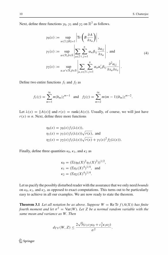
Next, define three functions γ0, γ1 and γ2 on RI as follows.

γ0(x) := supu∈I,‖B‖=1

∣∣∣∣Tr

(

B∂A

∂xu

)∣∣∣∣ ,

γ1(x) := supα∈R,β∈S

∣∣∣∣∣∣

∑

u∈I

n∑

i, j=1

αuβi j∂ai j

∂xu

∣∣∣∣∣∣, and

γ2(x) := supα,α′∈R,β∈S

∣∣∣∣∣∣

∑

u,v∈I

n∑

i, j=1

αuα′vβi j

∂2ai j

∂xu∂xv

∣∣∣∣∣∣.

(4)

Define two entire functions f1 and f2 as

f1(z) =∞∑

m=1

m|bm |zm−1 and f2(z) =∞∑

m=2

m(m − 1)|bm |zm−2.

Let λ(x) = ‖A(x)‖ and r(x) = rank(A(x)). Usually, of course, we will just haver(x) ≡ n. Next, define three more functions

η0(x) = γ0(x) f1(λ(x)),

η1(x) = γ1(x) f1(λ(x))√

r(x), and

η2(x) = γ2(x) f1(λ(x))√

r(x)+ γ1(x)2 f2(λ(x)).

Finally, define three quantities κ0, κ1, and κ2 as

κ0 = (E(η0(X)2η1(X)

2))1/2,

κ1 = (Eη1(X)4)1/4, and

κ2 = (Eη2(X)4)1/4.

Let us pacify the possibly disturbed reader with the assurance that we only need boundson κ0, κ1, and κ2, as opposed to exact computations. This turns out to be particularlyeasy to achieve in all our examples. We are now ready to state the theorem.

Theorem 3.1 Let all notation be as above. Suppose W = Re Tr f (A(X)) has finitefourth moment and let σ 2 = Var(W ). Let Z be a normal random variable with thesame mean and variance as W . Then

dT V (W, Z) ≤ 2√

5(c1c2κ0 + c31κ1κ2)

σ 2 .

123


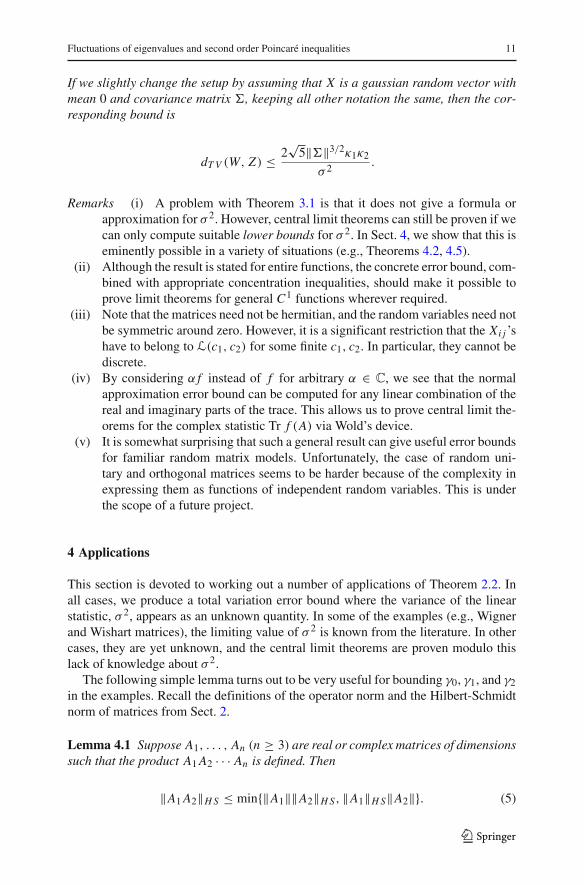
If we slightly change the setup by assuming that X is a gaussian random vector withmean 0 and covariance matrix �, keeping all other notation the same, then the cor-responding bound is

dT V (W, Z) ≤ 2√

5‖�‖3/2κ1κ2

σ 2 .

Remarks (i) A problem with Theorem 3.1 is that it does not give a formula orapproximation for σ 2. However, central limit theorems can still be proven if wecan only compute suitable lower bounds for σ 2. In Sect. 4, we show that this iseminently possible in a variety of situations (e.g., Theorems 4.2, 4.5).

(ii) Although the result is stated for entire functions, the concrete error bound, com-bined with appropriate concentration inequalities, should make it possible toprove limit theorems for general C1 functions wherever required.

(iii) Note that the matrices need not be hermitian, and the random variables need notbe symmetric around zero. However, it is a significant restriction that the Xi j ’shave to belong to L(c1, c2) for some finite c1, c2. In particular, they cannot bediscrete.

(iv) By considering α f instead of f for arbitrary α ∈ C, we see that the normalapproximation error bound can be computed for any linear combination of thereal and imaginary parts of the trace. This allows us to prove central limit the-orems for the complex statistic Tr f (A) via Wold’s device.

(v) It is somewhat surprising that such a general result can give useful error boundsfor familiar random matrix models. Unfortunately, the case of random uni-tary and orthogonal matrices seems to be harder because of the complexity inexpressing them as functions of independent random variables. This is underthe scope of a future project.

4 Applications

This section is devoted to working out a number of applications of Theorem 2.2. Inall cases, we produce a total variation error bound where the variance of the linearstatistic, σ 2, appears as an unknown quantity. In some of the examples (e.g., Wignerand Wishart matrices), the limiting value of σ 2 is known from the literature. In othercases, they are yet unknown, and the central limit theorems are proven modulo thislack of knowledge about σ 2.

The following simple lemma turns out to be very useful for bounding γ0, γ1, and γ2in the examples. Recall the definitions of the operator norm and the Hilbert-Schmidtnorm of matrices from Sect. 2.

Lemma 4.1 Suppose A1, . . . , An (n ≥ 3) are real or complex matrices of dimensionssuch that the product A1 A2 · · · An is defined. Then

‖A1 A2‖H S ≤ min{‖A1‖‖A2‖H S, ‖A1‖H S‖A2‖}. (5)

123

12 S. Chatterjee

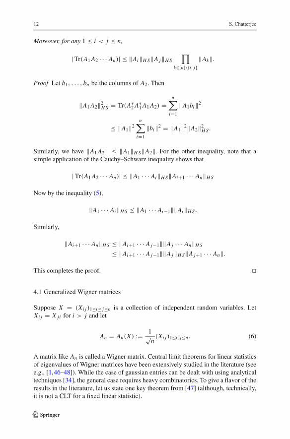
Moreover, for any 1 ≤ i < j ≤ n,

| Tr(A1 A2 · · · An)| ≤ ‖Ai‖H S‖A j‖H S

∏

k∈[n]\{i, j}‖Ak‖.

Proof Let b1, . . . , bn be the columns of A2. Then

‖A1 A2‖2H S = Tr(A∗

2 A∗1 A1 A2) =

n∑

i=1

‖A1bi‖2

≤ ‖A1‖2n∑

i=1

‖bi‖2 = ‖A1‖2‖A2‖2H S .

Similarly, we have ‖A1 A2‖ ≤ ‖A1‖H S‖A2‖. For the other inequality, note that asimple application of the Cauchy–Schwarz inequality shows that

| Tr(A1 A2 · · · An)| ≤ ‖A1 · · · Ai‖H S‖Ai+1 · · · An‖H S

Now by the inequality (5),

‖A1 · · · Ai‖H S ≤ ‖A1 · · · Ai−1‖‖Ai‖H S .

Similarly,

‖Ai+1 · · · An‖H S ≤ ‖Ai+1 · · · A j−1‖‖A j · · · An‖H S

≤ ‖Ai+1 · · · A j−1‖‖A j‖H S‖A j+1 · · · An‖.

This completes the proof. ��

4.1 Generalized Wigner matrices

Suppose X = (Xi j )1≤i≤ j≤n is a collection of independent random variables. LetXi j = X ji for i > j and let

An = An(X) := 1√n(Xi j )1≤i, j≤n . (6)

A matrix like An is called a Wigner matrix. Central limit theorems for linear statisticsof eigenvalues of Wigner matrices have been extensively studied in the literature (seee.g., [1,46–48]). While the case of gaussian entries can be dealt with using analyticaltechniques [34], the general case requires heavy combinatorics. To give a flavor of theresults in the literature, let us state one key theorem from [47] (although, technically,it is not a CLT for a fixed linear statistic).

123


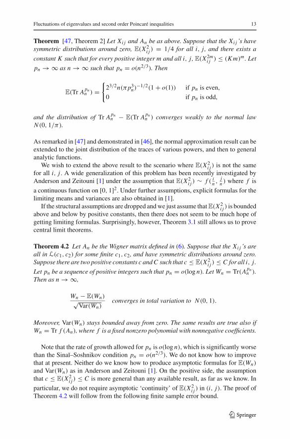
Theorem [47, Theorem 2] Let Xi j and An be as above. Suppose that the Xi j ’s havesymmetric distributions around zero, E(X2

i j ) = 1/4 for all i, j , and there exists a

constant K such that for every positive integer m and all i, j , E(X2mi j ) ≤ (K m)m. Let

pn → ∞ as n → ∞ such that pn = o(n2/3). Then

E(Tr Apnn ) =

{23/2n(πp3

n)−1/2(1 + o(1)) if pn is even,

0 if pn is odd,

and the distribution of Tr Apnn − E(Tr Apn

n ) converges weakly to the normal lawN (0, 1/π).

As remarked in [47] and demonstrated in [46], the normal approximation result can beextended to the joint distribution of the traces of various powers, and then to generalanalytic functions.

We wish to extend the above result to the scenario where E(X2i j ) is not the same

for all i, j . A wide generalization of this problem has been recently investigated byAnderson and Zeitouni [1] under the assumption that E(X2

i j ) ∼ f ( in ,

jn ) where f is

a continuous function on [0, 1]2. Under further assumptions, explicit formulas for thelimiting means and variances are also obtained in [1].

If the structural assumptions are dropped and we just assume that E(X2i j ) is bounded

above and below by positive constants, then there does not seem to be much hope ofgetting limiting formulas. Surprisingly, however, Theorem 3.1 still allows us to provecentral limit theorems.

Theorem 4.2 Let An be the Wigner matrix defined in (6). Suppose that the Xi j ’s areall in L(c1, c2) for some finite c1, c2, and have symmetric distributions around zero.Suppose there are two positive constants c and C such that c ≤ E(X2

i j ) ≤ C for all i, j .

Let pn be a sequence of positive integers such that pn = o(log n). Let Wn = Tr(Apnn ).

Then as n → ∞,

Wn − E(Wn)√Var(Wn)

converges in total variation to N (0, 1).

Moreover, Var(Wn) stays bounded away from zero. The same results are true also ifWn = Tr f (An), where f is a fixed nonzero polynomial with nonnegative coefficients.

Note that the rate of growth allowed for pn is o(log n), which is significantly worsethan the Sinaı̆–Soshnikov condition pn = o(n2/3). We do not know how to improvethat at present. Neither do we know how to produce asymptotic formulas for E(Wn)

and Var(Wn) as in Anderson and Zeitouni [1]. On the positive side, the assumptionthat c ≤ E(X2

i j ) ≤ C is more general than any available result, as far as we know. In

particular, we do not require asymptotic ‘continuity’ of E(X2i j ) in (i, j). The proof of

Theorem 4.2 will follow from the following finite sample error bound.

123

14 S. Chatterjee

Lemma 4.3 Fix n. Let A = A(X) be the Wigner matrix defined in (6). Suppose theXi j ’s are in L(c1, c2) for some finite c1, c2. Take an entire function f and define f1,f2 as in Theorem 3.1. Let λ denote the spectral radius of A. Let a = (E f1(λ)

4)1/4

and b = (E f2(λ)4)1/4. Suppose W = Re Tr f (A) has finite fourth moment and let

σ 2 = Var(W ). Let Z be a normal random variable with the same mean and varianceas W . Then

dT V (W, Z) ≤ 2√

5

σ 2

(4c1c2a2

√n

+ 8c31ab

n

)

.

Remarks (i) It is well known that under mild conditions, λ converges to a finitelimit as n → ∞ (see e.g., [4, Sect. 2.2.1]). Even exponentially decaying tailbounds are available [27]. Thus a and b are generally O(1) in the above bound.

(ii) Sinaı̆ and Soshnikov [46, Corollary 1] showed that σ 2 converges to a finite limitunder certain conditions on f and the distribution of the Xi j ’s. If these condi-tions are satisfied and the limit is nonzero, then we get a bound of order 1/

√n.

Moreover, for gaussian Wigner matrices we have c2 = 0 and hence a bound oforder 1/n. The difference between the gaussian and non-gaussian cases is notan accident. With f (z) = z, we have

Tr f (A) = 1√n

n∑

i=1

Xii .

In this case we know that the error bound in the non-gaussian case is exactly oforder 1/

√n.

Before proving Lemma 4.3, let us first prove Theorem 4.2 using the lemma. Themain difference between Lemma 4.3 and Theorem 4.2 is that the assumption of sym-metry on the distributions of the entries allows us to compute a lower bound on theunknown quantity σ 2 and actually prove a CLT in Theorem 4.2.

Proof of theorem 4.2 Let s2i j = E(X2

i j ), and let

ξi j = Xi j

si j.

Let �n denote the matrix 1√n(ξi j )1≤i, j≤n . Now take any collections of nonnegative

integers (αi j )1≤i≤ j≤n and (βi j )1≤i≤ j≤n . Then

Cov(∏

Xαi ji j ,

∏Xβi ji j

)=

(∏sαi j +βi ji j

) (∏E(ξ

αi j +βi ji j )−

∏E(ξ

αi ji j )E(ξ

βi ji j )

),

where the products are taken over 1 ≤ i ≤ j ≤ n. Now note that ifαi j +βi j is odd, then

E(ξαi j +βi ji j ) = E(ξ

αi ji j )E(ξ

βi ji j ) = 0. If αi j and βi j are both odd, then E(ξ

αi j +βi ji j ) ≥ 0

123


and E(ξαi ji j ) = E(ξ

βi ji j ) = 0. Finally, if αi j and βi j are both even, then

E(ξαi ji j )E(ξ

βi ji j ) ≤ (E(ξ

αi j +βi ji j ))

αi jαi j +βi j (E(ξ

αi j +βi ji j ))

βi jαi j +βi j = E(ξ

αi j +βi ji j ).

Thus, under all circumstances, we have

E(ξαi j +βi ji j ) ≥ E(ξ

αi ji j )E(ξ

βi ji j ) ≥ 0. (7)

Therefore,

Cov(∏

Xαi ji j ,

∏Xβi ji j

)≥ c

12

∑(αi j +βi j )Cov

(∏ξαi ji j ,

∏ξβi ji j

).

From this, it follows easily that for any positive integer pn ,

Var(Tr Apnn ) ≥ cpn Var(Tr�pn

n ).

Now, by (7),

Var(Tr�pnn ) ≥ 1

n pn

∑

1≤i1,...,i pn ≤n

Var(ξi1i2ξi2i3 · · · ξi pn i1).

If i1, . . . , i pn are distinct numbers, then

Var(ξi1i2ξi2i3 · · · ξi pn i1) = E(ξ2i1i2)E(ξ2

i2i3) · · · E(ξ2

i pn i1) = 1.

Thus,

Var(Tr�pnn ) ≥ n(n − 1) · · · (n − pn + 1)

n pn,

and so, if pn is a sequence of integers such that pn = o(n1/2), then

Var(Tr Apnn ) ≥ K cpn , (8)

where K is a positive constant that does not vary with n.Now note that for any nonnegative integer αi j , E(ξ

αi ji j ) ≥ 0. Thus,

E

(∏Xαi ji j

)=

∏sαi ji j E(ξ

αi ji j ) ≤ C

12

∑αi j E

(∏ξαi ji j

).

In particular, for any positive integer l,

E(Tr Al) ≤ Cl/2E(Tr�l

n).

123

16 S. Chatterjee

Let λn denote the spectral radius of An . Then for any positive integer m and anypositive even integer l,

E(λmn ) ≤

(E(Tr Alm

n ))1/ l ≤ Cm/2

(E(Tr�lm

n ))1/ l

.

Now let l = ln := 2[log n]. If mn is a sequence of positive integers such that mn =o(n2/3/ log n), it follows from the Sinaı̆–Soshnikov result stated above that for all n,

(E(Tr�lnmn

n ))1/ ln ≤ K ′2mn n1/ ln ≤ K 2mn ,

where K ′ and K are constants that do not depend on n. Note that we could applythe theorem because ξi j ’s are symmetric and E(ξ2m

i j ) ≤ (K m)m for all m due to

the L(c1, c2) assumption. The 2mn term arises because E(ξ2i j ) = 1 instead of 1/4 as

required in the Sinaı̆–Soshnikov theorem. Combined with the previous step, this gives

E(λmnn ) ≤ K (4C)mn/2. (9)

Now let us apply Lemma 4.3 to W = Tr Apnn . First, let us fix n. We have f (x) = x pn ,

and hence f1(x) = pn x pn−1 and f2(x) = pn(pn − 1)x pn−2. It follows that botha2 and ab are bounded by p2

n(E(λ4pnn ))1/2, which according to (9), is bounded by

K p2n(4C)pn . On the other hand, by (8), σ 2 is lower bounded by K cpn . Combining,

and using Lemma 4.3, we get

dT V (W, Z) ≤ K p2n√

n

(4C

c

)pn

,

where K is a constant depending only on c, C , c1 and c2, and Z is a gaussian randomvariable with the same mean and variance as W . If pn = o(log n), the bound goes tozero.

When Wn = Tr f (An), where f is a fixed polynomial with nonnegative coeffi-cients, the proof goes through almost verbatim, and is in fact simpler. The nonneg-ativity of the coefficients is required to ensure that all monomial terms are positivelycorrelated, so that we can get a lower bound on the variance. ��

Proof of Lemma 4.3 Let I = {(i, j) : 1 ≤ i ≤ j ≤ n}. Let x = (xi j )1≤i≤ j≤n denote atypical element of R

I. For each such x , let A(x) = (ai j (x))1≤i, j≤n denote the matrixwhose (i, j)th element is n−1/2xi j if i ≤ j and n−1/2x ji if i > j . Then the matrix Aconsidered above is simply A(X), and this puts us in the setting of Theorem 3.1. Now,

∂ai j

∂xkl=

{n−1/2 if (i, j) = (k, l) or (i, j) = (l, k),

0 otherwise.

123


Therefore, for any matrix B with ‖B‖ = 1, and 1 ≤ k �= l ≤ n,

∣∣∣∣Tr

(

B∂A

∂xkl

)∣∣∣∣ =

∣∣∣∣bkl + blk√

n

∣∣∣∣ ≤ 2√

n.

It is clear that the same bound holds even if k = l. Thus,

γ0(x) ≤ 2√n

for all x ∈ RI.

Next, let R and S be as in (3), and take anyα ∈ R,β ∈ S. Then by the Cauchy–Schwarzinequality, we have

∣∣∣∣∣∣

∑

(k,l)∈I

n∑

i, j=1

αklβi j∂ai j

∂xkl

∣∣∣∣∣∣≤ 1√

n

∑

(k,l)∈I

|αkl(βkl + βlk)| ≤ 2√n.

Thus,

γ1(x) ≤ 2√n

for all x ∈ RI.

Now, it is clear that γ2(x) ≡ 0 and r(x) ≤ n. Thus, if we define η0, η1, and η2 as inTheorem 3.1, and let λ(x) be the spectral radius of A(x), then for all x ∈ R

I we have

η0(x) ≤ 2 f1(λ(x))√n

,

η1(x) ≤ 2 f1(λ(x)), and

η2(x) ≤ 4 f2(λ(x))

n.

This gives

κ0 ≤ 4(E f1(λ)4)1/2√

n, κ1 ≤ 2(E f1(λ)

4)1/4, and κ2 ≤ 4(E f2(λ)4)1/4

n.

Plugging these values into Theorem 3.1, we get the result. ��

4.2 Gaussian matrices with correlated entries

Suppose we have a collection X = (Xi j )1≤i, j≤n of jointly gaussian random variableswith mean zero and n2 × n2 covariance matrix �. Let A = n−1/2(Xi j )1≤i, j≤n . Notethat A may be non-symmetric. Limiting behavior of the spectrum in such matriceshave been recently investigated by Anderson and Zeitouni [2] under special structureson �. We have the following general result.

123

18 S. Chatterjee

Proposition 4.4 Take an entire function f and define f1, f2 as in Theorem 3.1. Let λdenote the operator norm of A. Let a = (E f1(λ)

4)1/4 and b = (E f2(λ)4)1/4. Suppose

W = Re Tr f (A) has finite fourth moment and let σ 2 = Var(W ). Let Z be a normalrandom variable with the same mean and variance as W . Then

dT V (W, Z) ≤ 2√

5‖�‖3/2ab

σ 2n.

Proof The computations of κ1 and κ2 are exactly the same as for Wigner matrices.The only difference is that we now apply the second part of Theorem 3.1. ��

Of course, the limiting behavior of σ 2 is not known, so this does not prove a centrallimit theorem as long as such results are not established. The term ‖�‖3/2 can oftenbe handled by the well-known Gershgorin bound for the operator norm:

‖�‖ ≤ max1≤i, j≤n

n∑

k,l=1

|σi j,kl |,

where σi j,kl = Cov(Xi j , Xkl). The next example gives a concrete application of theabove result.

4.3 Gaussian Toeplitz matrices

Fix a number n and let X0, . . . , Xn−1 be independent standard gaussian random vari-ables. Let An be the matrix

An := n−1/2(X |i− j |)1≤i, j≤n .

This is a gaussian Toeplitz matrix, of the kind recently considered in Bryc et al. [13]and also in Meckes [40] and Bose and Sen [11]. Although Toeplitz determinants havebeen extensively studied (see e.g., Basor [7] and references therein), to the best of ourknowledge, there are no existing central limit theorems for general linear statistics ofeigenvalues of random Toeplitz matrices. We have the following result.

Theorem 4.5 Consider the gaussian Toeplitz matrices defined above. Let pn be asequence of positive integers such that pn = o(log n/ log log n). Let Wn = Tr(Apn

n ).Then, as n → ∞,

Wn − E(Wn)√Var(Wn)

converges in total variation to N (0, 1).

Moreover, there exists a positive constant C such that Var(Wn) ≥ (C/pn)pn n for

all n. The central limit theorem also holds for Wn = Tr f (An), when f is a fixednonzero polynomial with nonnegative coefficients. In that case, Var(Wn) ≥ Cn forsome positive constant C depending on f .

123


Remarks (i) Note that the theorem is only for gaussian Toeplitz matrices. In fact,considering the function f (x) = x , we see that a CLT need not always hold forlinear statistics of non-gaussian Toeplitz matrices.

(ii) This is an example of a matrix ensemble where nothing is known about thelimiting formula for Var(Wn). Theorem 3.1 enables us to prove the CLT evenwithout knowing the limit of Var(Wn). As before, this is possible because wecan easily get lower bounds on Var(Wn).

Proof In the notation of the previous subsection,

σi j,kl ={

1 if |i − j | = |k − l|,0 otherwise.

Thus,

‖�‖ ≤ maxi, j

∑

k,l

|σi j,kl | ≤ 2n.

Let λn denote the spectral norm of An . Using Proposition 4.4 and the above bound on‖�‖, we have

dT V (Wn, Zn) ≤ Cp2n(Eλ

4pnn )1/2

√n

Var(Wn), (10)

where Zn is a gaussian random variable with the same mean and variance as Wn andC is a universal constant.

In the rest of the argument we will write p instead of pn to ease notation. First,note that

Wn = Tr(Apn ) = n−p/2

∑

1≤i1,...,i p≤n

X |i1−i2| X |i2−i3| · · · X |i p−i1|.

As in the Proof of theorem 4.2, it is easy to verify that all terms in the above sumare positively correlated with each other, and hence, for any partition D of the set{1, . . . , n}p into disjoint subcollections,

Var(Wn) ≥ n−p∑

D∈D

Var

⎛

⎝∑

(i1,...,i p)∈D

X |i1−i2| X |i2−i3| · · · X |i p−i1|

⎞

⎠ . (11)

For any collection of distinct positive integers 1 ≤ a1, . . . , ap−1 ≤ �n/3p�, letDa1,...,ap−1 be the set of all 1 ≤ i1, . . . , i p ≤ n such that ik+1 − ik = ak for k =1, . . . , p − 1 and 1 ≤ i1 ≤ �n/3�. Clearly, |Da1,...,ap−1 | = �n/3�. Again, since the

123

20 S. Chatterjee

ai ’s are distinct,

Var

⎛

⎜⎝

∑

(i1,...,i p)∈Da1,...,ap−1

X |i1−i2| X |i2−i3| · · · X |i p−i1|

⎞

⎟⎠

= |Da1,...,ap−1 |2Var(Xa1 · · · Xap−1 Xa1+···+ap−1) = |Da1,...,ap−1 |2 ≥ n2

9.

Next, note that the number of ways to choose a1, . . . , ap−1 satisfying the restrictionsis

�n/3p�(�n/3p� − 1) · · · (�n/3p� − p + 2).

Since we can assume, without loss of generality, that n ≥ 4p2, the above quan-tity can be easily seen to be lower bounded by (n/12p)p−1. Finally, noting that if(a1, . . . , ap−1) �= (a′

1, . . . , a′p−1), then Da1,...,ap−1 and Da′

1,...,a′p−1

are disjoint, andapplying (11), we get

Var(Wn) ≥ n−p n p−1

(12p)p−1

n2

9≥ C pn

p p, (12)

where C is a positive universal constant.Next, let λn denote the spectral norm of An . By Theorem 1 of Meckes [40], we know

that E(λn) ≤ C√

log n. Now, it is easy to verify that the map (X0, . . . , Xn−1) �→ λn

has Lipschitz constant bounded irrespective of n. By standard gaussian concentrationresults (e.g., [39, Sects. 5.1–5.2]), it follows that for any k,

E|λn − E(λn)|k ≤ Ck/2kk/2,

where, again, C is a universal constant. Combining with result for E(λn), it followsthat for any n and k,

E(λkn) ≤ (Ck log n)k/2.

Thus, the term p2(Eλ4pn )

1/2 in (10) is bounded by p2(Cp log n)p. Therefore, from(10) and (12), it follows that

dT V (Wn, Zn) ≤ C p p2p+2(log n)p

√n

,

where C is a universal constant. Clearly, if p = o(log n/ log log n), this goes to zero.This completes the proof for Wn = Tr(Apn

n ). When Wn = Tr f (An), where f isa fixed polynomial with nonnegative coefficients, the proof goes through exactly asabove. If f (x) = c0 + · · · + ck xk , the nonnegativity of the coefficients ensures that

123


Var(Wn) ≥ c2k Var(Tr Ak

n), and we can re-use the bounds computed before to showthat Var(Wn) ≥ C( f )n. The rest is similar. ��

4.4 Wishart matrices

Let n ≤ N be two positive integers, and let X = (Xi j )1≤i≤n,1≤ j≤N be a collection ofindependent random variables in L(c1, c2) for some finite c1, c2. Let

A = N−1 X Xt .

In statistical parlance, the matrix A is called the Wishart matrix or sample covariancematrix corresponding to the data matrix X . Just as in the Wigner case, linear statisticsof eigenvalues of Wishart matrices also satisfy unnormalized central limit theoremsunder certain conditions. This was proved for polynomial f by Jonsson [36], and for amuch larger class of functions in Bai and Silverstein [6]. A different proof was recentlygiven by Anderson and Zeitouni [1]. We have the following error bound.

Proposition 4.6 Let λ be the largest eigenvalue of A. Take any entire function fand define f1, f2 as in Theorem 3.1. Let a = (E( f1(λ)

4λ2))1/4 and b = (E( f1(λ)+2n−1/2 f2(λ)λ)

4)1/4. Suppose W = Re Tr f (A) has finite fourth moment and let σ 2 =Var(W ). Let Z be a normal random variable with the same mean and variance as W .Then

dT V (W, Z) ≤ 8√

5

σ 2

(c1c2a2√n

N+ c3

1abn

N 3/2

)

.

If we now change the setup and assume that the entries of X are jointly gaussian withmean 0 and nN × nN covariance matrix�, keeping all other notation the same, thenthe corresponding bound is

dT V (W, Z) ≤ 8√

5‖�‖3/2abn

σ 2 N 3/2 .

Remarks (i) As in the Wigner case, it is well known that under mild conditions,λ = O(1) as n, N → ∞ with n/N → c ∈ [0, 1). We refer to Sect. 2.2.2 in thesurvey article [4] for details. It follows that a and b are O(1).

(ii) It is shown in [6] that in the case of independent entries, if n/N → c ∈ (0, 1),thenσ 2 converges to a finite positive constant under fairly general conditions (anexplicit formula for the limit is also available). Therefore under such conditions,the first bound above is of order 1/

√N .

(iii) We should remark that the spectrum of X Xt is often studied by studying theblock matrix

(0 XXt 0

)

,

123

22 S. Chatterjee

because

(0 XXt 0

)2

=(

X Xt 00 Xt X

)

.

Thus, in principle, we can derive Proposition 4.6 using the information contained inLemma 4.3. However, for expository purposes, we prefer carry out the explicit com-putations necessary for applying Theorem 3.1 without resorting to the above trick.The computations will also be helpful in dealing with the double Wishart case in thenext subsection.

Proof of Proposition 4.6 First, let us define the indexing set

I = {(p, q) : p = 1, . . . , n, q = 1, . . . , N }.

From now on, we simply write pq instead of (p, q). Let x = (x pq)pq∈I be a typicalelement of R

I. In the following, the collection x is used as a matrix, and it seems thatthe only way to avoid confusion is to write X instead of x , so we do that. Generally,there is no harm in confusing this X with the collection of random variables definedat the onset.

Let γ0, γ1, and γ2 be defined as in (4). For each m and i , let emi be the i th coordinatevector in R

m , i.e., the vector whose i th component is 1 and the rest are zero. Then

∂A

∂x pq= N−1(enpet

Nq Xt + XeNqetnp),

and

∂2 A

∂x pq∂xrs= N−1(enpet

NqeNsetnr + enr et

NseNqetnp)

={

N−1(enpetnr + enr et

np) if q = s,

0 otherwise.(13)

Now take any n × n matrix B with ‖B‖ = 1. Then for any p, q,

∣∣∣∣Tr

(

B∂A

∂x pq

)∣∣∣∣ = N−1| Tr(Benpet

Nq Xt + B XeNqetnp)|

= N−1|etNq Xt Benp + et

np B XeNq |

≤ 2N−1‖B‖‖X‖ = 2

√λ

N.

This shows that

γ0 ≤ 2

√λ

N.

123


Next, let α = (αpq)1≤p≤n,1≤q≤N , α′ = (αpq)1≤p≤n,1≤q≤N , and β = (βi j )1≤i, j≤n bearbitrary matrices of complex numbers such that ‖α‖H S = ‖α′‖H S = ‖β‖H S = 1.Then

∣∣∣∣∣∣

n∑

p=1

N∑

q=1

n∑

i, j=1

αpqβi j∂ai j

∂x pq

∣∣∣∣∣∣= N−1

∣∣∣∣∣∣

n∑

p=1

N∑

q=1

n∑

i, j=1

αpqβi j etni (enpet

Nq Xt +XeNqetnp)enj

∣∣∣∣∣∣

= N−1

∣∣∣∣∣∣

n∑

p=1

N∑

q=1

n∑

j=1

αpqβpj x jq +n∑

p=1

N∑

q=1

n∑

i=1

αpqβi pxiq

∣∣∣∣∣∣

= N−1∣∣Tr(αXtβ t )+Tr(αXtβ)

∣∣ .

By Lemma 4.1, we have

| Tr(αXtβ t )+ Tr(αXtβ)| ≤ 2‖α‖H S‖X‖‖β‖H S = 2√

Nλ.

Thus,

γ1 ≤ 2

√λ

N.

Again, by the formula (13) for second derivatives of A,

∣∣∣∣∣∣

n∑

p,r=1

N∑

q,s=1

n∑

i, j=1

αpqα′rsβi j

∂2ai j

∂x pq∂xrs

∣∣∣∣∣∣

= N−1

∣∣∣∣∣∣

n∑

p,r=1

N∑

q=1

n∑

i, j=1

αpqα′rqβi j e

tni (enpet

nr + enr etnp)enj

∣∣∣∣∣∣

= N−1

∣∣∣∣∣∣

n∑

p,r=1

N∑

q=1

αpqα′rq(βpr + βr p)

∣∣∣∣∣∣

= N−1∣∣∣Tr(αα′tβ t )+ Tr(αα′tβ)

∣∣∣ ≤ 2N−1‖α‖H S‖α′‖H S‖β‖H S .

This shows that

γ2 ≤ 2

N.

Finally, note that rank(A) ≤ n. Combining the bounds we get

η0 ≤ 2 f1(λ)

√λ

N, η1 ≤ 2 f1(λ)

√λn

N, and η2 ≤ 2 f1(λ)

√n

N+ 4 f2(λ)λ

N.

123

24 S. Chatterjee

From this, we get

κ0 ≤ 4√

n

N(E( f1(λ)

4λ2))1/2,

κ1 ≤ 2√

n√N(E( f1(λ)

4λ2))1/4, and

κ2 ≤ 2√

n

N(E( f1(λ)+ 2n−1/2 f2(λ)λ)

4)1/4.

With the aid of Theorem 3.1, this completes the proof. ��

4.5 Double Wishart matrices

Let n ≤ N ≤ M be three positive integers, and let X = (Xi j )1≤i≤n,1≤ j≤N beand Y = (Yi j )1≤i≤n,1≤ j≤M be two collections of independent random variables inL(c1, c2) for some finite c1, c2. Let

A = X Xt (Y Y t )−1.

A matrix like A is called a double Wishart matrix. Double Wishart matrices are veryimportant in statistical theory of canonical correlations (see the Discussion in Sect. 2.2of [35]).

If the matrices X and Y had independent standard gaussian entries, the matrixX Xt (X Xt + Y Y t )−1 would be known as a Jacobi matrix. In a recent preprint, Jiang[32] proves the CLT for the Jacobi ensemble. We have the following result.

Proposition 4.7 Let λx and λy be the largest eigenvalues of N−1 X Xt and M−1Y Y t ,and let δy be the smallest eigenvalue of M−1Y Y t . Let λ = max{1, λx , λy, δ

−1y }. Take

any entire function f and define f1, f2 as in Theorem 3.1. Let a = (E( f1(λ)4λ14))1/4

and

b = (E(4 f1(λ)λ5 + 2n−1/2 f2(λ)λ

7)4)1/4.

Suppose W = Re Tr f (A) has finite fourth moment and let σ 2 = Var(W ). Let Z be anormal random variable with the same mean and variance as W . Then

dT V (W, Z) ≤ 4√

10

σ 2

(c1c2a2 N

√n

M2 + 2c31ab

√Nn

M2

)

.

Remarks (i) Assume that n, N , and M grow to infinity at the same rate (we referto this as the ‘large dimensional limit’). From the results about the extremeeigenvalues of Wishart matrices ([4, Sect. 2.2.2]), it is clear that λ = O(1), andhence a, b are stochastically bounded.

123


(ii) There are no rigorous results about the behavior of σ 2 in the large dimensionallimit, other than in the gaussian case, which has been settled in [32], where itis shown that σ 2 converges to a finite limit.

(iii) When the entries of X and Y are jointly gaussian and some conditions on thedimensions are satisfied, the exact joint distribution of the eigenvalues of A isknown (see [35], Sect. 2.2 for references and an interesting story). While it maybe possible to derive a CLT for the gaussian case using the explicit form of thisdensity, it is hard to see how the non-gaussian case can be handled by either themethod of moments or Stieltjes transforms.

(iv) In principle, it seems something could be said using the second order freenessresults of Mingo and Speicher [41]. However, to the best of our knowledge, anexplicit CLT for double Wishart matrices has not been worked out using secondorder freeness.

Proof of Proposition 4.7 For convenience, let C = X Xt and D = Y Y t . Note that‖C‖ = ‖X‖2 = Nλx , ‖D‖ = ‖Y‖2 = Mλy and ‖D−1‖ = 1/(Mδy). Let the othernotation be as in the proof of Proposition 4.6. Now

∂A

∂x pq= (enpet

Nq Xt + XeNqetnp)D

−1.

Again, using the formula

∂D−1

∂ypq= −D−1 ∂D

∂ypqD−1,

we have

∂A

∂ypq= −C D−1(enpet

MqY t + Y eMqetnp)D

−1.

Now take any n × n matrix B with ‖B‖ = 1. Then for any p, q,

∣∣∣∣Tr

(

B∂A

∂x pq

)∣∣∣∣ = | Tr(Benpet

Nq Xt D−1 + B XeNqetnp D−1)|

= |etNq Xt D−1 Benp + et

np D−1 B XeNq |≤ 2‖D−1‖‖X‖≤ 2λ3/2

√N

M.

Similarly,

∣∣∣∣Tr

(

B∂A

∂ypq

)∣∣∣∣ ≤ 2‖C‖‖Y‖‖D−1‖2 ≤ 2λ7/2 N

M3/2 .

123

26 S. Chatterjee

Since λ ≥ 1 and N ≤ M ,

γ0 ≤ 2λ7/2√

N

M.

Next, let αn×N , α̃n×M , α′n×N , α̃′

n×M , and βn×n be arbitrary arrays of complex numberssuch that ‖α‖2

H S + ‖α̃‖2H S = 1, ‖α′‖2

H S + ‖α̃′‖2H S = 1, and ‖β‖H S = 1. Then

∣∣∣∣∣∣

n∑

p=1

N∑

q=1

n∑

i, j=1

αpqβi j∂ai j

∂x pq

∣∣∣∣∣∣

=∣∣∣∣∣∣

n∑

p=1

N∑

q=1

n∑

i, j=1

αpqβi j etni (enpet

Nq Xt + XeNqetnp)D

−1enj

∣∣∣∣∣∣

=∣∣∣∣∣∣

n∑

p=1

N∑

q=1

n∑

j=1

αpqβpj (Xt D−1)q j +

n∑

p=1

N∑

q=1

n∑

i, j=1

αpqβi j xiq(D−1)pj

∣∣∣∣∣∣

=∣∣∣Tr(αXt D−1β t )+ Tr(D−1β t Xαt )

∣∣∣

≤ 2‖α‖H S‖β‖H S‖X‖‖D−1‖ ≤ 2‖α‖H Sλ3/2

√N

M.

Similarly,

∣∣∣∣∣∣

n∑

p=1

M∑

q=1

n∑

i, j=1

α̃pqβi j∂ai j

∂ypq

∣∣∣∣∣∣

=∣∣∣∣∣∣

n∑

p=1

M∑

q=1

n∑

i, j=1

α̃pqβi j etni C D−1(enpet

MqY t + Y eMqetnp)D

−1enj

∣∣∣∣∣∣

=∣∣∣∣∣∣

n∑

p=1

M∑

q=1

n∑

i, j=1

(α̃pqβi j (C D−1)i p(Y

t D−1)q j + α̃pqβi j (C D−1Y )iq(D−1)pj

)∣∣∣∣∣∣

=∣∣∣Tr(α̃Y t D−1β t C D−1)+ Tr(C D−1Y α̃t D−1β t )

∣∣∣

≤ 2‖α̃‖H S‖β‖H S‖Y‖‖C‖‖D−1‖2 ≤ 2‖α̃‖H Sλ7/2 N

M3/2 .

Combining, and using the inequality

‖α‖H S + ‖α̃‖H S ≤√

2(‖α‖2H S + ‖α̃‖2

H S) = √2,

123


we get

γ1 ≤ 2√

2λ7/2√

N

M.

Next, let us compute the second derivatives. First, note that

∂2 A

∂x pq∂xrs= (enpet

NqeNsetnr + enr et

NseNqetnp)D

−1

={(enpet

nr + enr etnp)D

−1 if q = s,

0 otherwise.

Using Lemma 4.1 in the last step below, we get

∣∣∣∣∣∣

n∑

p,r=1

N∑

q,s=1

n∑

i, j=1

αpqα′rsβi j

∂2ai j

∂x pq∂xrs

∣∣∣∣∣∣

=∣∣∣∣∣∣

n∑

p,r=1

N∑

q=1

n∑

i, j=1

αpqα′rqβi j e

tni (enpet

nr + enr etnp)D

−1enj

∣∣∣∣∣∣

=∣∣∣∣∣∣

n∑

p,r=1

N∑

q=1

n∑

j=1

αpqα′rqβpj (D

−1)r j +n∑

p,r=1

N∑

q=1

n∑

j=1

αpqα′rqβr j (D

−1)pj )

∣∣∣∣∣∣

=∣∣∣Tr(αα′t D−1β t )+ Tr(αα′tβ(D−1)t )

∣∣∣

≤ 2‖α‖H S‖α′‖H S‖β‖H S‖D−1‖.

Thus, we have

∣∣∣∣∣∣

n∑

p,r=1

N∑

q,s=1

n∑

i, j=1

αpqαrsβi j∂2ai j

∂x pq∂xrs

∣∣∣∣∣∣≤ 2‖α‖H S‖α′‖H Sλ

M. (14)

Next, note that

∂2 A

∂x pq∂yrs= −(enpet

Nq Xt + XeNqetnp)D

−1(enr etMsY t + Y eMset

nr )D−1.

123

28 S. Chatterjee

When we open up the brackets in the above expression, we get four terms. Let us dealwith the first term:

∣∣∣∣∣∣

n∑

p,r=1

N∑

q=1

M∑

s=1

n∑

i, j=1

αpq α̃′rsβi j e

tni (enpet

Nq Xt D−1enr etMsY t D−1)enj

∣∣∣∣∣∣

=∣∣∣∣∣∣

n∑

p,r=1

N∑

q=1

M∑

s=1

n∑

j=1

αpq α̃′rsβpj (X

t D−1)qr (Yt D−1)s j

∣∣∣∣∣∣

=∣∣∣Tr(αXt D−1α̃′Y t D−1β)

∣∣∣ ≤ ‖α‖H S‖α̃′‖H S

λ3√

N

M3/2 .

It can be similarly verified that the same bound holds for the other three terms as well.Combining, we get

∣∣∣∣∣∣

n∑

p,r=1

N∑

q=1

M∑

s=1

n∑

i, j=1

αpq α̃′rsβi j

∂2ai j

∂x pq∂yrs

∣∣∣∣∣∣≤ 4‖α‖H S‖α̃′‖H S

λ3√

N

M3/2 . (15)

Finally, note that

∂2 A

∂ypq∂yrs= C D−1(enpet

NqY t + Y eNqetnp)D

−1(enr etNsY t + Y eNset

nr )D−1

+ C D−1(enr etNsY t + Y eNset

nr )D−1(enpet

NqY t + Y eNqetnp)D

−1

− C D−1(enpetnr + enr et

np)D−1

I{q=s}.

Proceeding exactly as before, it is quite easy to get the following bound. It seemsreasonable to omit the details.

∣∣∣∣∣∣

n∑

p,r=1

M∑

q,s=1

n∑

i, j=1

α̃pq α̃′rsβi j

∂2ai j

∂ypq∂yrs

∣∣∣∣∣∣≤ 10‖α̃‖H S‖α̃′‖H S

λ5 N

M2 . (16)

Combining (14), (15), and (16), and noting that N ≤ M , λ ≥ 1, and the HS-norms ofα, α′, α̃, and α̃′ are all bounded by 1, it is now easy to get that

γ2 ≤ 16λ5

M.

Finally, note that rank(A) ≤ n. Combining everything we get

η0 ≤ 2 f1(λ)λ7/2

√N

M, η1 ≤ 2

√2 f1(λ)λ

7/2√

Nn

M,

and η2 ≤ 12 f1(λ)λ5√n

M+ 8 f2(λ)λ

7 N

M2 .

123


From this, we get

κ0 ≤ 4N√

2n

M2 (E( f1(λ)4λ14))1/2,

κ1 ≤ 2√

2Nn

M(E( f1(λ)

4λ14))1/4, and

κ2 ≤ 4√

n

M(E(4 f1(λ)λ

5 + 2n−1/2 f2(λ)λ7)4)1/4.

An application of Theorem 3.1 completes the proof. ��

5 Proofs

5.1 Proof of Theorem 2.2

The following basic lemma due to Charles Stein is our connection with Stein’s method.For the reader’s convenience, we reproduce the proof.

Lemma 5.1 ([50, p. 25]) Let Z be a standard gaussian random variable. Then forany random variable W , we have

dT V (W, Z) ≤ sup{|E(ψ(W )W − ψ ′(W ))| : ‖ψ ′‖∞ ≤ 2}.

Proof Take any u : R → [−1, 1]. It can be verified that the function

ϕ(x) = ex2/2

x∫

−∞e−t2/2(u(t)− Eu(Z))dt

= −ex2/2

∞∫

x

e−t2/2(u(t)− Eu(Z))dt

is a solution to the equation

ϕ′(x)− xϕ(x) = u(x)− Eu(Z).

Thus for each x ,

ϕ′(x) = u(x)− Eu(Z)− xex2/2

∞∫

x

e−t2/2(u(t)− Eu(Z))dt.

123

30 S. Chatterjee

It follows that

supx≥0

|ϕ′(x)| ≤ (sup |u(x)− Eu(Z)|)⎛

⎝1 + supx≥0

xex2/2

∞∫

x

e−t2/2dt

⎞

⎠

≤ 2 sup |u(x)− Eu(Z)| ≤ 4.

It can be verified that the same bound holds for supx≤0 |ϕ′(x)| by replacing x with−x . Therefore, we have

|Eu(W )− Eu(Z)| = |E(ϕ(W )W − ϕ′(W ))|≤ sup{|E(ψ(W )W − ψ ′(W ))| : ‖ψ ′‖∞ ≤ 4}.

Since

dT V (W, Z) = 1

2sup{|Eu(W )− Eu(Z)| : ‖u‖∞ ≤ 1},

this completes the proof. ��The next lemma is for technical convenience.

Lemma 5.2 It suffices to prove Theorem 2.2 under the assumption that g, ∇g and∇2g are uniformly bounded.

Proof Suppose we have proved Theorem 2.2 under the said assumption. Take anyg ∈ C2(Rn) such that σ 2 is finite. Now, if any one among κ0, κ1, and κ2 is infinite,there is nothing to prove. So let us assume that they are all finite.

Let h : R+ → [0, 1] be a C∞ function such that h(t) = 1 when t ≤ 1 and h(t) = 0

when t ≥ 2. For each α > 0 let

gα(x) = g(x)h(α−1‖x‖).

Clearly, as α → ∞,

dT V (g(X), gα(X)) ≤ P(g(X) �= gα(X)) ≤ P(‖X‖ > α) → 0. (17)

Note that for any finite α, gα and its derivatives are uniformly bounded over Rn . Now,

since Eg(X)2 is finite, |gα(x)| ≤ |g(x)| for all x , and gα converges to g pointwise,the dominated convergence theorem gives

limα→∞ Egα(X) = Eg(X), and lim

α→∞ Egα(X)2 = Eg(X)2.

Again, since Eg(X)4 and κ0, κ1 and κ2 are all finite, the same logic shows that

limα→∞ κi (gα) = κi (g) for i = 0, 1, 2.

123


These three steps combined show that if Theorem 2.2 holds for each gα , it must holdfor g as well. This completes the proof. ��

The following result is the main ingredient in the proof of Theorem 2.2.

Lemma 5.3 Let Y = (Y1, . . . ,Yn) be a vector of i.i.d. standard gaussian random vari-ables. Let f : R

n → R be an absolutely continuous function such that W = f (Y )has zero mean and unit variance. Assume that f and its derivatives have subexpo-nential growth at infinity. Let Y ′ be an independent copy of Y and define the functionT : R

n → R as

T (y) :=1∫

0

1

2√

tE

(n∑

i=1

∂ f

∂yi(y)

∂ f

∂yi(√

t y + √1 − tY ′)

)

dt

Let h(w) = E(T (Y )|W = w). Then Eh(W ) = 1. If Z is standard gaussian, then

dT V (W, Z) ≤ 2E|h(W )− 1| ≤ 2[Var(T (Y ))]1/2,

where dT V is the total variation distance.

Proof Take any ψ : R → R so that ψ ′ exists and is bounded. Then we have

E(ψ(W )W ) = E(ψ( f (Y )) f (Y )− ψ( f (Y )) f (Y ′))

= E

⎛

⎝

1∫

0

ψ( f (Y ))d

dtf (

√tY +√

1 − tY ′)dt

⎞

⎠

= E

⎛

⎝

1∫

0

ψ( f (Y ))n∑

i=1

(Yi

2√

t− Y ′

i

2√

1 − t

)∂ f

∂yi(√

tY +√1 − tY ′)dt

⎞

⎠ .

Now fix t ∈ (0, 1), and let Ut = √tY +√

1 − tY ′, and Vt = √1 − tY −√

tY ′. Then Ut

and Vt are independent standard gaussian random vectors and Y = √tUt +

√1 − tVt .

Taking any i , and using the integration-by-parts formula for the gaussian measure (ingoing from the second to the third line below), we get

E

(

ψ( f (Y ))

(Yi

2√

t− Y ′

i

2√

1 − t

)∂ f

∂yi(√

tY + √1 − tY ′)

)

= 1

2√

t (1 − t)E

(

ψ( f (√

tUt + √1 − tVt ))Vt,i

∂ f

∂yi(Ut )

)

= 1

2√

tE

(

ψ ′( f (Y ))∂ f

∂yi(Y )

∂ f

∂yi(Ut )

)

.

Note that we need the growth condition on the derivatives of f to carry out the inter-change of expectation and integration and the integration-by-parts. From the above,

123

32 S. Chatterjee

we have

E(ψ(W )W ) = E

⎛

⎝ψ ′(W )

1∫

0

1

2√

t

n∑

i=1

∂ f

∂yi(Y )

∂ f

∂yi(√

tY + √1 − tY ′)dt

⎞

⎠

= E(ψ ′(W )T (Y )) = E(ψ ′(W )h(W )).

The assertion that E(h(W )) = 1 now follows by taking ψ(w) = w and using thehypothesis that E(W 2) = 1. Also, easily, we have the upper bound

|E(ψ(W )W − ψ ′(W ))| = |E(ψ ′(W )(h(W )− 1))|≤ ‖ψ ′‖∞E|h(W )− 1|.

A simple application of Lemma 5.1 completes the proof. ��

Theorem 2.2 follows from the above lemma if we bound Var(T (Y )) using thegaussian Poincaré inequality, as we do below.

Proof of Theorem 2.2 First off, by Lemma 5.2, we can assume that g, ∇g, and ∇2gare uniformly bounded and hence apply Lemma 5.3 without having to check forthe growth conditions at infinity. Let Y1, . . . ,Yn be independent standard gaussianrandom variables and ϕ1, . . . , ϕn be functions such that Xi = ϕi (Yi ) and ‖ϕ′

i‖∞ ≤ c1,‖ϕ′′

i ‖∞ ≤ c2 for each i . Define a function ϕ : Rn → R

n as ϕ(y1, . . . , yn) :=(ϕ1(y1), . . . , ϕn(yn)) and let

f (y) := g(ϕ(y)).

Then W = g(X) = f (Y ). It is not difficult to see, through centering and scaling, thatit suffices to prove Theorem 2.2 under the assumptions that E(W ) = 0 and E(W 2) = 1(this is where the σ 2 appears in the error bound). Now define T as in Lemma 5.3:

T (y) =1∫

0

1

2√

tE

(n∑

i=1

∂ f

∂yi(y)

∂ f

∂yi(√

t y + √1 − tY ′)

)

dt,

where Y ′ is an independent copy of Y . Our strategy for bounding Var(T ) is to simplyuse the gaussian Poincaré inequality:

Var(T (Y )) ≤ E‖∇T (Y )‖2.

123


The boundedness of ∇2g ensures that we can move the derivative inside the integralswhen differentiating T :

∂T

∂yi(y) = E

1∫

0

1

2√

t

n∑

j=1

∂2 f

∂yi∂y j(y)

∂ f

∂y j(√

t y + √1 − tY ′)dt

+ E

1∫

0

1

2

n∑

j=1

∂ f

∂y j(y)

∂2 f

∂yi∂y j(√

t y + √1 − tY ′)dt.

Now for each t ∈ [0, 1], let Ut = √tY + √

1 − tY ′. With several applications ofJensen’s inequality and the inequality (a + b)2 ≤ 2a2 + 2b2, we get

E‖∇T (Y )‖2 ≤ E

1∫

0

1√t

n∑

i=1

⎛

⎝n∑

j=1

∂2 f

∂yi∂y j(Y )

∂ f

∂y j(Ut )

⎞

⎠

2

dt

+ E

1∫

0

1

2

n∑

i=1

⎛

⎝n∑

j=1

∂ f

∂y j(Y )

∂2 f

∂yi∂y j(Ut )

⎞

⎠

2

dt (18)

Now, we have

∂ f

∂yi(y) = ∂g

∂xi(ϕ(y))ϕ′

i (yi ).

Thus, if i �= j ,

∂2 f

∂yi∂y j= ∂2g

∂xi∂x j(ϕ(y))ϕ′

i (yi )ϕ′j (y j ).

On the other hand,

∂2 f

∂y2i

= ∂2g

∂x2i

(ϕ(y))ϕ′i (yi )

2 + ∂g

∂xi(ϕ(y))ϕ′′

i (yi ).

Thus, for any y, u ∈ Rn ,

n∑

i=1

⎛

⎝n∑

j=1

∂2 f

∂yi∂y j(y)

∂ f

∂y j(u)

⎞

⎠

2

≤ 2n∑

i=1

⎛

⎝n∑

j=1

∂2g

∂xi∂x j(ϕ(y))ϕ′

i (yi )ϕ′j (y j )

∂g

∂x j(ϕ(u))ϕ′

j (u j )

⎞

⎠

2

123

34 S. Chatterjee

+ 2n∑

i=1

(∂g

∂xi(ϕ(y))ϕ′′

i (yi )∂g

∂xi(ϕ(u))ϕ′

i (ui )

)2

≤ 2c61‖∇2g(ϕ(y))‖2‖∇g(ϕ(u))‖2 + 2c2

1c22

n∑

i=1

(∂g

∂xi(ϕ(y))

∂g

∂xi(ϕ(u))

)2

.

Let us now fix t ∈ [0, 1], replace y by Y and u by Ut and use the above inequality tobound the first integrand on the right hand side of (18). First, note that since Ut hasthe same law as Y ,

E(‖∇2g(ϕ(Y ))‖2‖∇g(ϕ(Ut ))‖2)

≤ (E‖∇2g(ϕ(Y ))‖4)1/2(E‖∇g(ϕ(Ut ))‖4)1/2

= (E‖∇2g(X)‖4)1/2(E‖∇g(X)‖4)1/2 = κ21κ

22 .

For the same reason, we also have

n∑

i=1

E

[(∂g

∂xi(ϕ(Y ))

∂g

∂xi(ϕ(Ut ))

)2]

≤ κ20 .

Combining, we get

E

n∑

i=1

⎛

⎝n∑

j=1

∂2 f

∂yi∂y j(Y )

∂ f

∂y j(Ut )

⎞

⎠

2

≤ 2c61κ

21κ

22 + 2c2

1c22κ

20 .

Since this does not depend on t , it is now easy to see that the first term on the righthand side is bounded by 4c6

1κ21κ

22 + 4c2

1c22κ

20 . In a very similar manner, the second

term can be bounded by c61κ

21κ

22 + c2

1c22κ

20 . Combining, and applying the inequality√

a + b ≤ √a + √

b, we finish the proof of first part of the theorem.To prove the second part, let X = AY , where Y is a vector of independent standard

gaussian random variables and A is a matrix such that � = AAt . Define h : Rn → R

as h(y) = g(Ay). It is easy to verify that

‖∇h(y)‖ ≤ ‖�‖1/2‖∇g(Ay)‖ and ‖∇2h(y)‖ ≤ ‖�‖‖∇2g(Ay)‖.

The rest is straightforward from the first part of the theorem applied to h(Y ) insteadof g(X), noting that for the standard gaussian distribution we have c1 = 1 and c2 = 0.

��

5.2 Proof of Theorem 3.1

Let us begin with some bounds on matrix differentials. Inequality (5) from Lemma 4.1is particularly useful.

123


Lemma 5.4 Let A = (ai j )1≤i, j≤n be an arbitrary square matrix with complex entries.Let f (z) = ∑∞

m=0 bm zm be an entire function. Define two associated entire functionsf1 and f2 as f1(z) = ∑∞

m=1 m|bm |zm−1 and f2(z) = ∑∞m=2 m(m − 1)|bm |zm−2.

Then for each i, j , we have

∂

∂ai jTr( f (A)) = ( f ′(A)) j i .

This gives the bounds

∣∣∣∣∂

∂ai jTr( f (A))

∣∣∣∣ ≤ f1(‖A‖) for each i, j , and

∑

i, j

∣∣∣∣∂

∂ai jTr( f (A))

∣∣∣∣

2

≤ rank(A) f1(‖A‖)2.

Next, for each 1 ≤ i, j, k, l ≤ n, let

hi j,kl = ∂2

∂ai j∂aklTr( f (A)).

Let H be the n2 × n2 matrix (hi j,kl)1≤i, j,k,l≤n. Then ‖H‖ ≤ f2(‖A‖).

Proof For each i , let ei be the i th coordinate vector in Rn , i.e., the vector whose i th

component is 1 and the rest are zero. Take any integer m ≥ 1. A simple computationgives

∂

∂ai jTr(Am) =

m−1∑

r=0

Tr

(

Ar ∂A

∂ai jAm−r−1

)

= m Tr

(∂A

∂ai jAm−1

)

.

Thus,

∂

∂ai jTr( f (A)) = Tr

(∂A

∂ai jf ′(A)

)

= Tr(ei etj f ′(A)) = ( f ′(A)) j i .

The first inequality follows from this, since |( f ′(A)) j i | ≤ ‖ f ′(A)‖ ≤ f1(‖A‖). Next,recall that if B is a square matrix and r = rank(B), then ‖B‖H S ≤ √

r‖B‖. Thisholds because

‖B‖2H S =

∑

i

λ2i ,

123

36 S. Chatterjee

where λi are the singular values of B, whereas ‖B‖ = maxi |λi |. Thus, if we letr = rank(A), then

⎛

⎝∑

i, j

∣∣∣∣∂

∂ai jTr( f (A))

∣∣∣∣

2⎞

⎠

1/2

= ‖ f ′(A)‖H S ≤∞∑

m=1

m|bm |‖Am−1‖H S

≤ √r

∞∑

m=1

m|bm |‖Am−1‖ ≤ √r

∞∑

m=1

m|bm |‖A‖m−1 = √r f1(‖A‖).

This proves the first claim. Next, fix some m ≥ 2. Another simple computation showsthat

∂2

∂ai j∂aklTr(Am) = m

m−2∑

r=0

Tr

(∂A

∂ai jAr ∂A

∂aklAm−r−2

)

= mm−2∑

r=0

Tr(ei etj Ar eket

l Am−r−2).

Now let B = (bi j )1≤i, j≤n and C = (ci j )1≤i, j≤n be arbitrary arrays of complex num-bers such that

∑i, j |bi j |2 = ∑

i, j |ci j |2 = 1. Using the above expression, we get

∑

i, j,k,l

bi j ckl∂2

∂ai j∂aklTr(Am) = m

m−2∑

r=0

Tr(B Ar C Am−r−2).

Now, by Lemma 4.1, it follows that

| Tr(B A1C A2)| ≤ ‖B‖H S‖C‖H S‖A1‖‖A2‖ ≤ ‖A‖m−2.

Thus,

∣∣∣∣∣∣

∑

i, j,k,l

bi j cklhi j,kl

∣∣∣∣∣∣≤

∞∑

m=2

m(m − 1)|bm |‖A‖m−2 = f2(‖A‖).

Since this holds for all B,C such that∑

i, j |bi j |2 = ∑i, j |ci j |2 = 1, the proof is done.

��Proof of Theorem 3.1 Let all notation be as in the statement of the theorem. For anyn × n matrix B, let ψ(B) = Tr f (B). Define the map g : R

I → C as g = ψ ◦ A, thatis,

g(x) = Tr f (A(x)).

123


It is useful to recall the following basic fact for the subsequent computations: For anyk and any vector x ∈ C

k ,

‖x‖ = sup{∣∣∣∑k

1xi yi

∣∣∣ : y ∈ C

k, ‖y‖ = 1}. (19)

Using this and the definition of γ1 we get

‖∇g(x)‖= supα∈R

∣∣∣∣∣∣

∑

u∈I

αu∂g

∂xu(x)

∣∣∣∣∣∣

= supα∈R

∣∣∣∣∣∣

∑

u∈I

n∑

i, j=1

αu∂ψ

∂ai j(A(x))

∂ai j

∂xu(x)

∣∣∣∣∣∣≤γ1(x)

⎛

⎝n∑

i, j=1

∣∣∣∣∂ψ

∂ai j(A(x))

∣∣∣∣

2⎞

⎠

1/2

.

Now suppose f1 is defined as in Lemma 5.4. Applying the second bound fromLemma 5.4 to the last term in the above expression, we get

‖∇g(x)‖ ≤ γ1(x) f1(‖A(x)‖)√rank(A(x)) = η1(x). (20)

Again note that for any u ∈ I, by Lemma 5.4 and the definition of γ0, we have

∣∣∣∣∂g

∂xu(x)

∣∣∣∣ =

∣∣∣∣Tr

(

f ′(A) ∂A

∂xu

)∣∣∣∣ ≤ γ0(x) f1(‖A(x)‖) = η0(x).

Thus,

∑

u∈I

∣∣∣∣∂g

∂xu(x)

∣∣∣∣

4

≤ maxu∈I

∣∣∣∣∂g

∂xu(x)

∣∣∣∣

2 ∑

u∈I

∣∣∣∣∂g

∂xu(x)

∣∣∣∣

2

≤ η0(x)2η1(x)

2. (21)

Next, note that

∂2g

∂xu∂xv=

n∑

i, j=1

∂ψ

∂ai j(A(x))

∂2ai j

∂xu∂xv(x)+

n∑

i, j,k,l=1

∂2ψ

∂ai j∂akl(A(x))

∂ai j

∂xu(x)

∂akl

∂xv(x).

Thus, if ∇2g denotes the Hessian matrix of g, then

‖∇2g(x)‖ = supα,α′∈R

∣∣∣∣∣∣

∑

u,v∈I

αuα′v

∂2g

∂xu∂xv

∣∣∣∣∣∣

≤ supα,α′∈R

∣∣∣∣∣∣

∑

u,v∈I

n∑

i, j=1

αuα′v

∂ψ

∂ai j(A(x))

∂2ai j

∂xu∂xv(x)

∣∣∣∣∣∣

+ supα,α′∈R

∣∣∣∣∣∣

∑

u,v∈I

n∑

i, j,k,l=1

αuα′v

∂2ψ

∂ai j∂akl(A(x))

∂ai j

∂xu(x)

∂akl

∂xv(x)

∣∣∣∣∣∣.

123

38 S. Chatterjee

Now, by the definition of γ2(x) and Lemma 5.4, we have

supα,α′∈R

∣∣∣∣∣∣

∑

u,v∈I

n∑

i, j=1

αuα′v

∂ψ

∂ai j(A(x))

∂2ai j

∂xu∂xv(x)

∣∣∣∣∣∣

≤ γ2(x)

⎛

⎝n∑

i, j=1

∣∣∣∣∂ψ

∂ai j(A(x))

∣∣∣∣

2⎞

⎠

1/2

≤ γ2(x) f1(‖A(x)‖)√rank(A(x)).

For the second term, note that by the definition of the operator norm and the identity(19),

supα,α′∈R

∣∣∣∣∣∣

∑

u,v∈I

n∑

i, j,k,l=1

αuα′v

∂2ψ

∂ai j∂akl(A(x))

∂ai j

∂xu(x)

∂akl

∂xv(x)

∣∣∣∣∣∣

≤ ‖∇2ψ(A(x))‖ supα∈R

n∑

i, j=1

∣∣∣∣∣∣

∑

u∈I

αu∂ai j

∂xu(x)

∣∣∣∣∣∣

2

= ‖∇2ψ(A(x))‖ supα∈R,β∈S

∣∣∣∣∣∣

n∑

i, j=1

∑

u∈I

αuβi j∂ai j

∂xu(x)

∣∣∣∣∣∣

2

.

Using the third bound from Lemma 5.4 and the definition of γ1(x), we now get

supα,α′∈R

∣∣∣∣∣∣

∑

u,v∈I

n∑

i, j,k,l=1

αuα′v

∂2ψ

∂ai j∂akl(A(x))

∂ai j

∂xu(x)

∂akl

∂xv(x)

∣∣∣∣∣∣≤ f2(‖A(x)‖)γ1(x)

2.

Combining the bounds obtained in the last two steps, we have

‖∇2g(x)‖ ≤ γ2(x) f1(‖A(x)‖)√rank(A(x))+ γ 21 (x) f2(‖A(x)‖)

= η2(x). (22)

Finally, since g is defined on a real domain, therefore ∇ Re g = Re ∇g and ∇2 Re g =Re ∇2g. Thus, ‖∇ Re g(x)‖ ≤ ‖∇g(x)‖ and ‖∇2 Re g(x)‖ ≤ ‖∇2g(x)‖. The proofis now completed by using (20), (21), and (22) to bound κ1, κ0, and κ2 in Theorem 2.2.The second part follows from the second part of Theorem 2.2. ��Acknowledgment The author is grateful to Persi Diaconis for many helpful remarks and suggestions,and to the referee for suggesting a number of key improvements.

References

1. Anderson, G., Zeitouni, O.: A CLT for a band matrix model. Probab. Theory Related Fields 134(2), 283–338 (2006)

123


2. Anderson, G., Zeitouni, O.: A law of large numbers for finite range dependent random matrices.Preprint. Available at http://arxiv.org/math/0609364, (2006)

3. Avram, F., Bertsimas, D.: On central limit theorems in geometrical probability. Ann. Appl. Pro-bab. 3(4), 1033–1046 (1993)

4. Bai, Z.D.: Methodologies in spectral analysis of large-dimensional random matrices, a review. Stat.Sinica 9(3), 611–677 (1999)

5. Bai, Z.D., Yao, J.-F.: On the convergence of the spectral empirical process of Wigner matrices. Preprint(2003)

6. Bai, Z.D., Silverstein, J.W.: CLT for linear spectral statistics of large-dimensional sample covariancematrices. Ann. Probab. 32, 533–605 (2004)

7. Basor, E.L.: Toeplitz determinants, Fisher–Hartwig symbols, and random matrices. Recent perspec-tives in random matrix theory and number theory, pp. 309–336. London Math. Soc. Lecture Note Ser.,vol. 322. Cambridge University Press, Cambridge (2005)

8. Basor, E., Chen, Y.: Perturbed Hankel determinants. J. Phys. A 38(47), 10101–10106 (2005)9. Bickel, P.J., Breiman, L.: Sums of functions of nearest neighbor distances, moment bounds, limit

theorems and a goodness of fit test. Ann. Probab. 11(1), 185–214 (1983)10. Borovkov, A.A., Utev, S.A.: An inequality and a characterization of the normal distribution connected

with it. Teor. Veroyatnost. Primenen. 28(2), 209–218 (1983)11. Bose, A., Sen, A.: Spectral norm of random large dimensional noncentral Toeplitz and Hankel matrices.

Electron. Commun. Probab. 12, 29–35 (2007) (electronic)12. Boutetde Monvel, A., Pastur, L., Shcherbina, M.: On the statistical mechanics approach in the random

matrix theory: Integrated density of states. J. Stat. Phys. 7, 585–611 (1995)13. Bryc, W., Dembo, A., Jiang, T.: Spectral measure of large random Hankel, Markov, and Toeplitz

matrices. Ann. Probab. 34(1), 1–38 (2006)14. Cabanal-Duvillard, T.: Fluctuations de la loi empirique de grande matrices aléatoires. Ann. Inst. H.

Poincaré Probab. Stat. 37, 373–402 (2001)15. Cacoullos, T., Papathanasiou, V., Utev, S.A.: Variational inequalities with examples and an application

to the central limit theorem. Ann. Probab. 22(3), 1607–1618 (1994)16. Chatterjee, S.: A new method of normal approximation. Ann. Probab. Available at http://arxiv.org/abs/

math/0611213, (2006) (to appear)17. Chen, L.H.Y.: The central limit theorem and Poincaré-type inequalities. Ann. Probab. 16(1), 300–304

(1988)18. Chernoff, H.: A note on an inequality involving the normal distribution. Ann. Probab. 9(3), 533–535

(1981)19. Costin, O., Lebowtz, J.: Gaussian fluctuations in random matrices. Phys. Rev. Lett. 75, 69–72 (1995)20. Diaconis, P., Shahshahani, M.: On the eigenvalues of random matrices: Studies in applied probabil-

ity. J. Appl. Probab. 31A, 49–62 (1994)21. Diaconis, P., Evans, S.N.: Linear functionals of eigenvalues of random matrices. Trans. Am. Math.

Soc. 353, 615–2633 (2001)22. Dumitriu, I., Edelman, A.: Global spectrum fluctuations for the β-Hermite and β-Laguerre ensembles

via matrix models. J. Math. Phys. 47(6), 063302–063336 (2006)23. Friedrich, K.O.: A Berry–Esseen bound for functions of independent random variables. Ann.

Stat. 17(1), 170–183 (1989)24. Girko, V.L.: Theory of Random Determinants. Kluwer, Dordrecht (1990)25. Goldstein, L., Reinert, G.: Stein’s method and the zero bias transformation with application to simple

random sampling. Ann. Appl. Probab. 7(4), 935–952 (1997)26. Guionnet, A.: Large deviations upper bounds and central limit theorems for non-commutative func-

tionals of Gaussian large random matrices. Ann. Inst. H. Poincaré Probab. Stat. 38, 341–384 (2002)27. Guionnet, A., Zeitouni, O.: Concentration of the spectral measure for large matrices. Electron. Comm.

Probab. 5, 119–136 (2000)28. Hachem, W., Khorunzhiy, O., Loubaton, P., Najim, J., Pastur, L.: A new approach for capacity analysis

of large dimensional multi-antenna channels. Preprint (2006)29. Hachem, W., Loubaton, P., Najim, J.: A CLT for information-theoretic statistics of Gram random

matrices with a given variance profile. Preprint (2007)30. Hughes, C.P., Keating, J.P., O’Connell, N.: On the characteristic polynomial of a random unitary

matrix. Commun. Math. Phys. 220, 429–451 (2000)

123

http://arxiv.org/math/0609364

http://arxiv.org/abs/math/0611213

http://arxiv.org/abs/math/0611213

40 S. Chatterjee

31. Israelson, S.: Asymptotic fuctuations of a particle system with singular interaction. Stoch. Process.Appl. 93, 25–56 (2001)

32. Jiang, T.: Approximation of Haar distributed matrices and limiting distributions of eigenvalues ofJacobi Ensembles. Preprint (2006)

33. Johansson, K.: On random matrices from the classical compact groups. Ann. Math. 145(2), 519–545(1997)

34. Johansson, K.: On the fluctuation of eigenvalues of random Hermitian matrices. Duke Math. J. 91,151–204 (1998)

35. Johnstone, I.M.: High dimensional statistical inference and random matrices. Proc. ICM 2006 (toappear) (2006)

36. Jonsson, D.: Some limit theorems for the eigenvalues of a sample covariance matrix. J. Mult.Anal. 12, 1–38 (1982)

37. Keating, J.P., Snaith, N.C.: Random matrix theory and ζ(1/2 + i t). Commun. Math. Phys. 214, 57–89(2000)

38. Khorunzhy, A.M., Khoruzhenko, B.A., Pastur, L.A.: Asymptotic properties of large random matriceswith independent entries. J. Math. Phys. 37, 5033–5060 (1996)

39. Ledoux, M.: The Concentration of Measure Phenomenon, volume 89 of Mathematical Surveys andMonographs. American Mathematical Society, Providence (2001)

40. Meckes, M.W.: On the spectral norm of a random Toeplitz matrix. Preprint. Available at http://arxiv.org/pdf/math/0703134, (2006)

41. Mingo, J.A., Speicher, R.: order freeness and fluctuations of random matrices. I. Gaussian and Wishartmatrices and cyclic Fock spaces. J. Funct. Anal. 235(1), 226–270 (2006)

42. Muckenhoupt, B.: Hardy’s inequality with weights. Studia Math. 44, 31–38 (1972)43. Rider, B., Virág, B.: The noise in the circular law and the Gaussian free field. Available at http://arxiv.

org/math.PR/0606663, (2006)44. Rider, B., Silverstein, J.W.: Gaussian fluctuations for non-Hermitian random matrix ensembles. Ann.

Probab. (to appear) (2006)45. Rüschendorf L.: Projections and iterative procedures. In: Krishnaiah, P.R. (ed.) Multivariate Analysis

VI, pp. 485–493. North-Holland, Amsterdam (1985)46. Sinaı̆, Ya., Soshnikov, A.: Central limit theorems for traces of large random matrices with independent

entries. Bol. Soc. Brasil. Mat. 29, 1–24 (1998)47. Sinaı̆, Ya., Soshnikov, A.: A refinement of Wigner’s semicircle law in a neighborhood of the spectrum

edge for random symmetric matrices. Funct. Anal. Appl. 32(2), 114–131 (1998)48. Soshnikov, A.: Gaussian limits for determinantal random point fields. Ann. Probab. 28, 171–181 (2002)49. Stein, C.: A bound for the error in the normal approximation to the distribution of a sum of depen-

dent random variables. In: Proc. of the Sixth Berkeley Symp. on Math. Statist. and Probab., Vol. II:Probability theory, pp. 583–602 (1972)

50. Stein, C.: Approximate computation of expectations. IMS Lecture Notes—Monograph Series, vol. 7(1986)

51. van Zwet, W.R.: A Berry–Esseen bound for symmetric statistics. Z. Wahrsch. Verw. Gebiete 66(3),425–440 (1984)

52. Wieand, K.: Eigenvalue distributions of random unitary matrices. Probab. Theory RelatedFields 123, 202–224 (2002)

123

http://arxiv.org/pdf/math/0703134

http://arxiv.org/pdf/math/0703134

http://arxiv.org/math.PR/0606663

http://arxiv.org/math.PR/0606663

Documents

Fluctuations of eigenvalues and second order Poincaré inequalities