D. Lacoste

Laboratoire Physico-Chimie Théorique,

UMR Gulliver, ESPCI, Paris

Fluctuation theorems: where do we go from here ?

Outline of the talk  

1.  Fluctuation theorems for systems out of equilibrium 2.  Modified fluctuation-dissipation theorems out of equilibrium 3.  Fluctuations theorems for systems at equilibrium

4.  Non-invasive estimation of dissipation

Fluctuation theorems for systems out of equilibrium

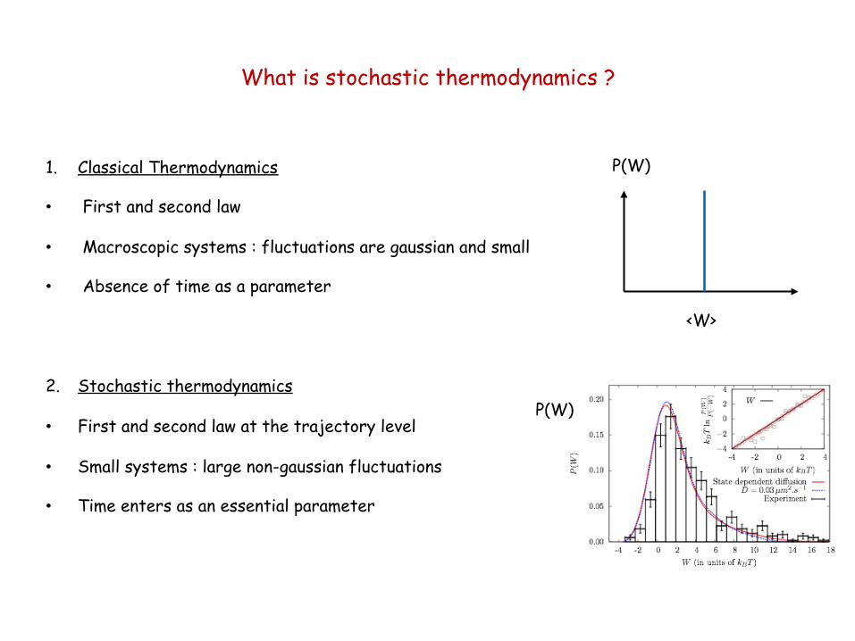
1.  Classical Thermodynamics

•  First and second law •  Macroscopic systems : fluctuations are gaussian and small

•  Absence of time as a parameter 2.  Stochastic thermodynamics

•  First and second law at the trajectory level •  Small systems : large non-gaussian fluctuations

•  Time enters as an essential parameter

What is stochastic thermodynamics ?

P(W)

<W>

P(W)

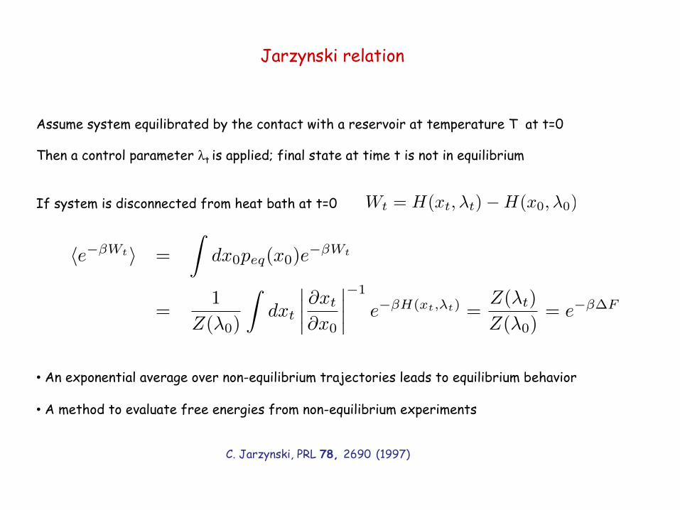
Assume system equilibrated by the contact with a reservoir at temperature T at t=0 Then a control parameter lt is applied; final state at time t is not in equilibrium If system is disconnected from heat bath at t=0 •  An exponential average over non-equilibrium trajectories leads to equilibrium behavior

•  A method to evaluate free energies from non-equilibrium experiments

Jarzynski relation

Wt = H(xt,�t)�H(x0,�0)

he��Wti =

Zdx0peq(x0)e

��Wt

=1

Z(�0)

Zdxt

����@xt

@x0

�����1

e

��H(xt,�t) =Z(�t)

Z(�0)= e

���F

C. Jarzynski, PRL 78, 2690 (1997)

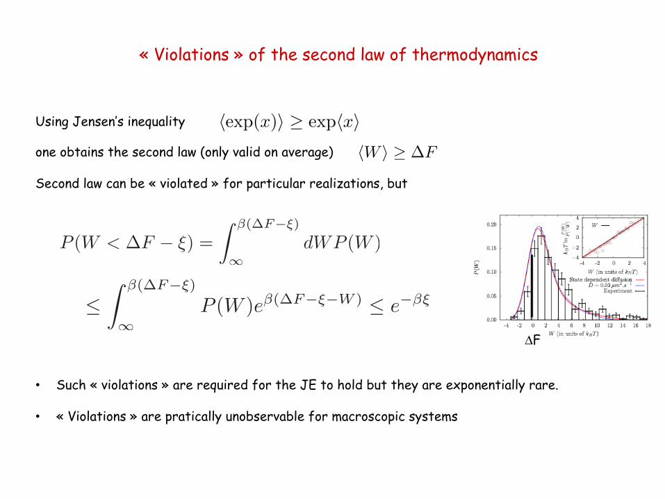
Using Jensen’s inequality one obtains the second law (only valid on average) Second law can be « violated » for particular realizations, but •  Such « violations » are required for the JE to hold but they are exponentially rare.

•  « Violations » are pratically unobservable for macroscopic systems

« Violations » of the second law of thermodynamics

hexp(x)i � exphxihW i � �F

P (W < �F � ⇠) =

Z �(�F�⇠)

1dWP (W )

Z �(�F�⇠)

1P (W )e�(�F�⇠�W ) e��⇠

DF

Systems in contact with a thermostat

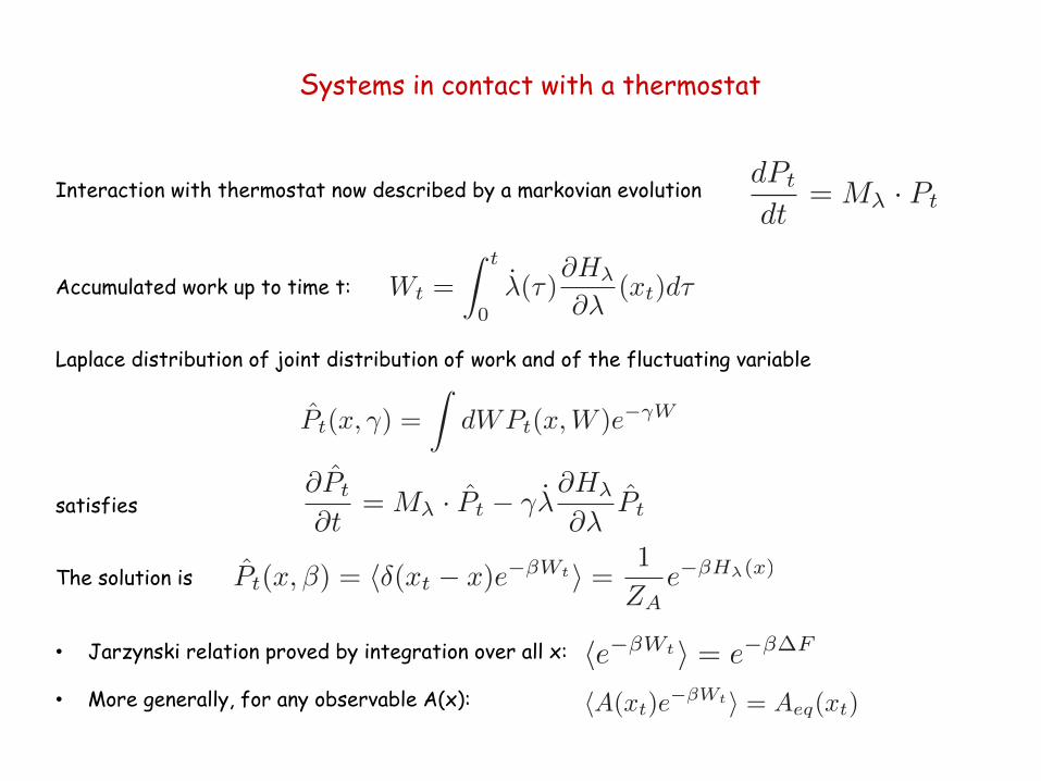
Interaction with thermostat now described by a markovian evolution Accumulated work up to time t: Laplace distribution of joint distribution of work and of the fluctuating variable satisfies The solution is •  Jarzynski relation proved by integration over all x:

•  More generally, for any observable A(x):

dPt

dt= M� · Pt

Wt =

Z t

0�̇(⌧)

@H�

@�(xt)d⌧

P̂t(x, �) =

ZdWPt(x,W )e��W

@P̂t

@t= M� · P̂t � ��̇

@H�

@�P̂t

P̂t(x,�) = h�(xt � x)e��Wti = 1

ZAe

��H�(x)

hA(xt)e��Wti = Aeq(xt)

he��Wti = e���F

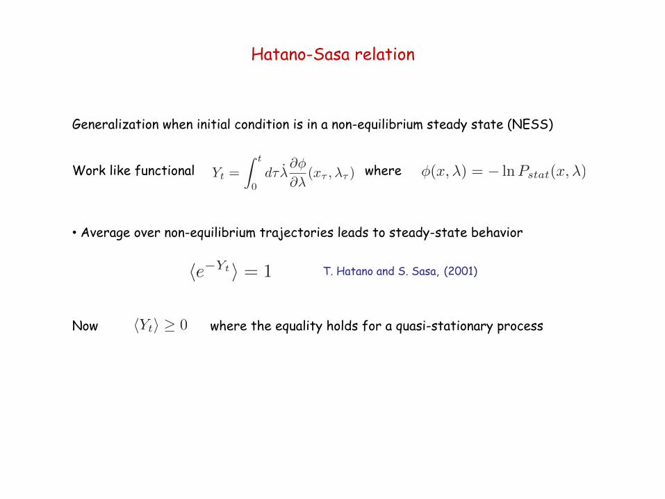
Generalization when initial condition is in a non-equilibrium steady state (NESS) Work like functional where •  Average over non-equilibrium trajectories leads to steady-state behavior

Now where the equality holds for a quasi-stationary process

Hatano-Sasa relation

T. Hatano and S. Sasa, (2001)

Yt =

Z t

0d⌧ �̇

@�

@�

(x⌧ ,�⌧ ) �(x,�) = � lnPstat(x,�)

he�Yti = 1

hYti � 0

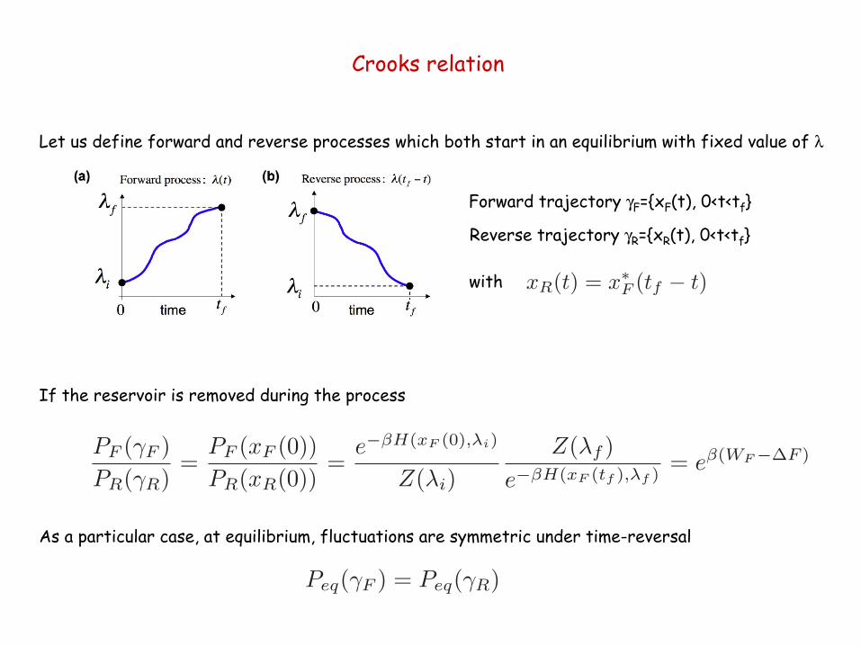
Let us define forward and reverse processes which both start in an equilibrium with fixed value of l

Forward trajectory gF={xF(t), 0<t<tf} Reverse trajectory gR={xR(t), 0<t<tf}

with If the reservoir is removed during the process As a particular case, at equilibrium, fluctuations are symmetric under time-reversal

Crooks relation

Peq(�F ) = Peq(�R)

xR(t) = x

⇤F (tf � t)

PF (�F )

PR(�R)=

PF (xF (0))

PR(xR(0))=

e

��H(xF (0),�i)

Z(�i)

Z(�f )

e

��H(xF (tf ),�f )= e

�(WF��F )

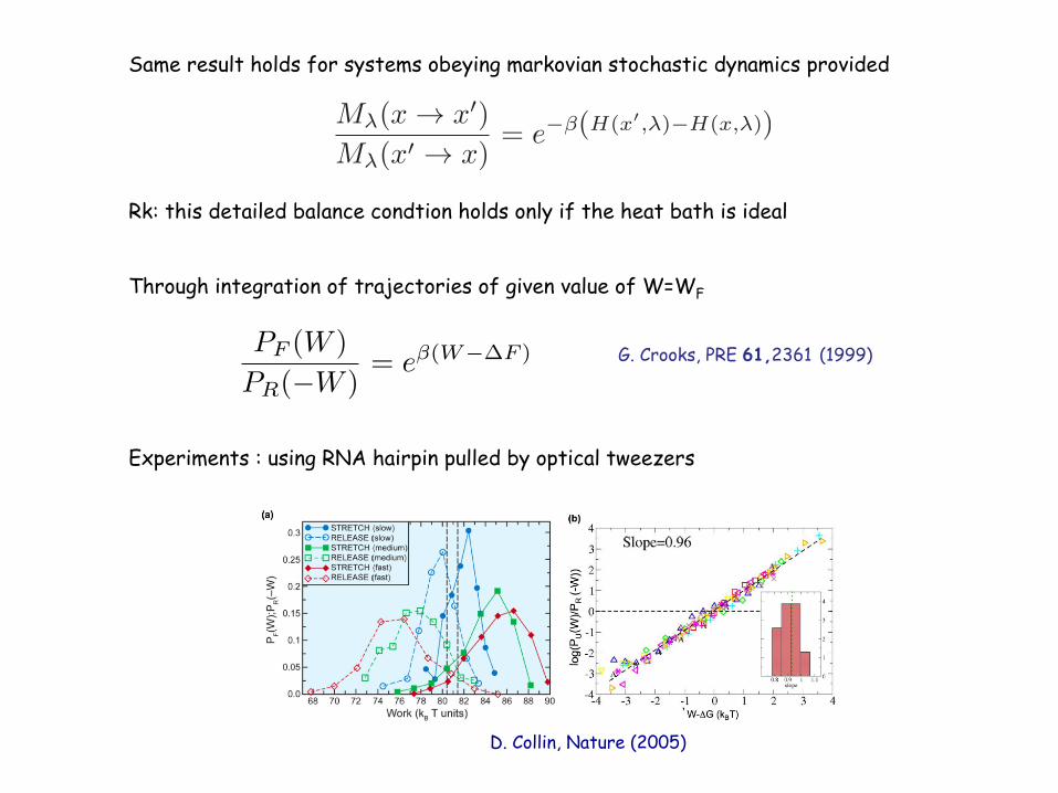
Same result holds for systems obeying markovian stochastic dynamics provided Rk: this detailed balance condtion holds only if the heat bath is ideal Through integration of trajectories of given value of W=WF Experiments : using RNA hairpin pulled by optical tweezers

D. Collin, Nature (2005)

G. Crooks, PRE 61,2361 (1999) PF (W )

PR(�W )= e�(W��F )

M�(x ! x

0)

M�(x0 ! x)= e

��(H(x0,�)�H(x,�))

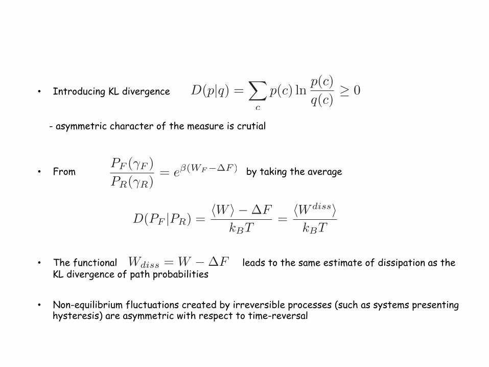
•  Introducing KL divergence

- asymmetric character of the measure is crutial

•  From by taking the average

•  The functional leads to the same estimate of dissipation as the KL divergence of path probabilities

•  Non-equilibrium fluctuations created by irreversible processes (such as systems presenting hysteresis) are asymmetric with respect to time-reversal

D(p|q) =X

c

p(c) lnp(c)

q(c)� 0

D(PF |PR) =hW i ��F

kBT=

hW dissikBT

PF (�F )

PR(�R)= e�(WF��F )

Wdiss = W ��F

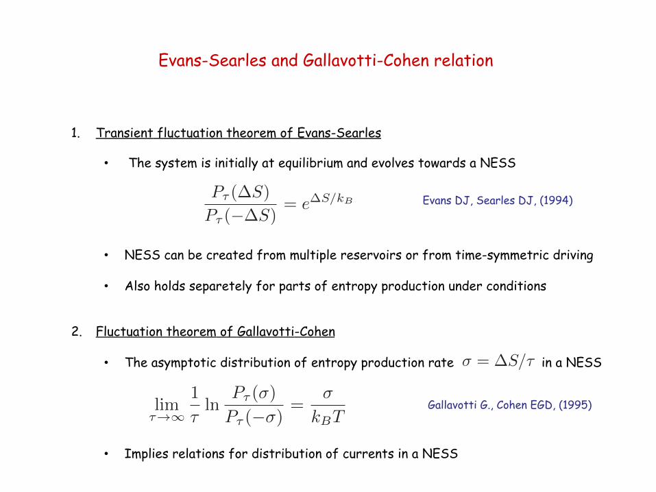
1.  Transient fluctuation theorem of Evans-Searles

•  The system is initially at equilibrium and evolves towards a NESS

•  NESS can be created from multiple reservoirs or from time-symmetric driving

•  Also holds separetely for parts of entropy production under conditions 2.  Fluctuation theorem of Gallavotti-Cohen

•  The asymptotic distribution of entropy production rate in a NESS

•  Implies relations for distribution of currents in a NESS

Evans-Searles and Gallavotti-Cohen relation

P⌧ (�S)

P⌧ (��S)= e�S/kB

� = �S/⌧

lim⌧!1

1

⌧ln

P⌧ (�)

P⌧ (��)=

�

kBT

Evans DJ, Searles DJ, (1994)

Gallavotti G., Cohen EGD, (1995)

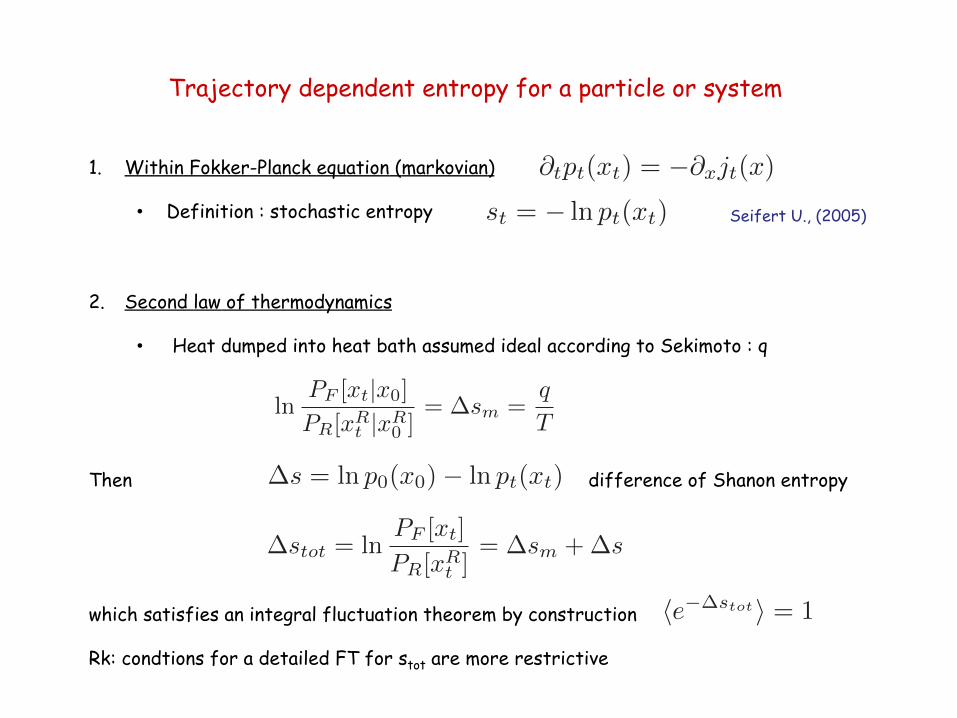
Trajectory dependent entropy for a particle or system

1.  Within Fokker-Planck equation (markovian)

•  Definition : stochastic entropy

2.  Second law of thermodynamics

•  Heat dumped into heat bath assumed ideal according to Sekimoto : q

Then difference of Shanon entropy which satisfies an integral fluctuation theorem by construction Rk: condtions for a detailed FT for stot are more restrictive

st = � ln pt(xt)

@

t

p

t

(xt

) = �@

x

j

t

(x)

Seifert U., (2005)

lnPF [xt|x0]

PR[xRt |xR

0 ]= �sm =

q

T

�s = ln p0(x0)� ln pt(xt)

�s

tot

= lnP

F

[xt

]

P

R

[xR

t

]= �s

m

+�s

he��stoti = 1

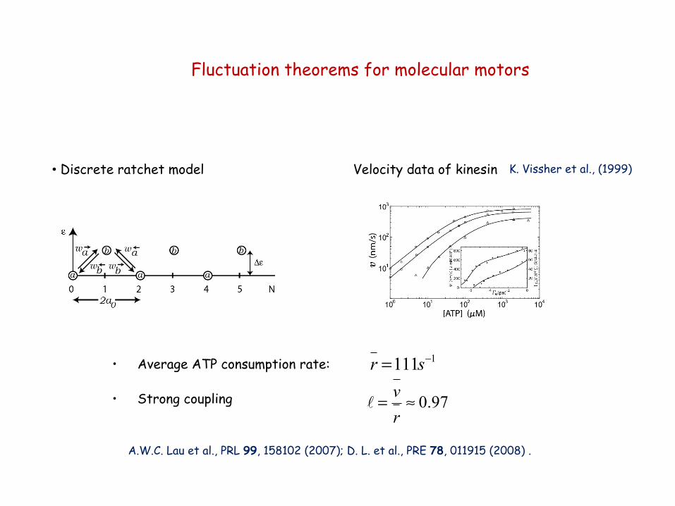
•  Discrete ratchet model Velocity data of kinesin

K. Vissher et al., (1999)

ℓ = vr≈ 0.97

1111r s−= •  Average ATP consumption rate:

•  Strong coupling

A.W.C. Lau et al., PRL 99, 158102 (2007); D. L. et al., PRE 78, 011915 (2008) .

Fluctuation theorems for molecular motors

•  Statistics of the displacement n(t) and of the number of ATP molecules consumed y(t) as function of external and chemical loads ?

•  At thermodynamic equilibrium: f=0 and Dµ=0 , fluctuations of n(t) and y(t) are gaussian, characterized by two diffusion coefficients D1 and D2

•  Near equilibrium: for small f and Dµ=0, linear response theory holds,

Einstein relations: L11=D1 and L22=D2

Onsager relations: L12=L21 •  What happens far from equilibrium ?

Minimal ratchet: thermodynamics

Velocity (mechanical current) v( f ,Δµ) = limt→∞

d n(t)dt( )

( , ) limt

d y tr f

dtµ

→∞Δ =ATP consumption rate (chemical current)

11 12

21 22

v L f L

r L f L

µµ

= + Δ

= + Δ

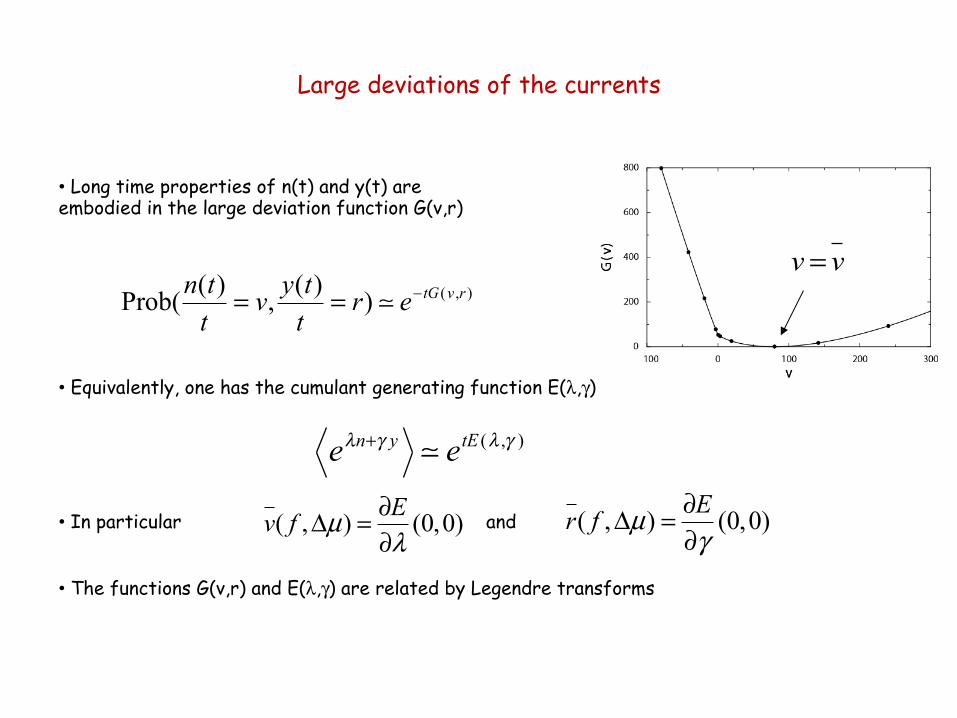
•  Long time properties of n(t) and y(t) are embodied in the large deviation function G(v,r)

•  Equivalently, one has the cumulant generating function E(l,g)

•  In particular and

•  The functions G(v,r) and E(l,g) are related by Legendre transforms

Large deviations of the currents

Prob(n(t)t

= v, y(t)t

= r) ! e− tG(v ,r )

eλn+γ y ! etE (λ ,γ )

( , ) (0,0)Ev f µλ∂Δ =∂

v v=

( , ) (0,0)Er f µγ

∂Δ =∂

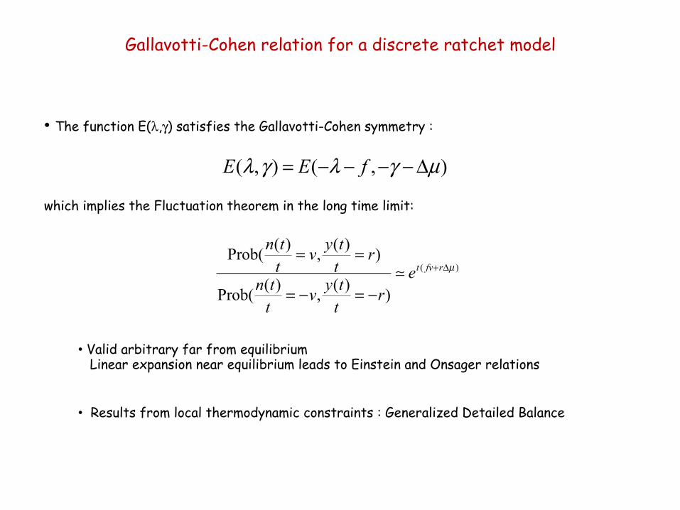
•  The function E(l,g) satisfies the Gallavotti-Cohen symmetry :

which implies the Fluctuation theorem in the long time limit:

•  Valid arbitrary far from equilibrium Linear expansion near equilibrium leads to Einstein and Onsager relations

•  Results from local thermodynamic constraints : Generalized Detailed Balance

Gallavotti-Cohen relation for a discrete ratchet model

( , ) ( , )E E fλ γ λ γ µ= − − − −Δ

Prob(n(t)t

= v, y(t)t

= r)

Prob(n(t)t

= −v, y(t)t

= −r)! et ( fv+rΔµ )

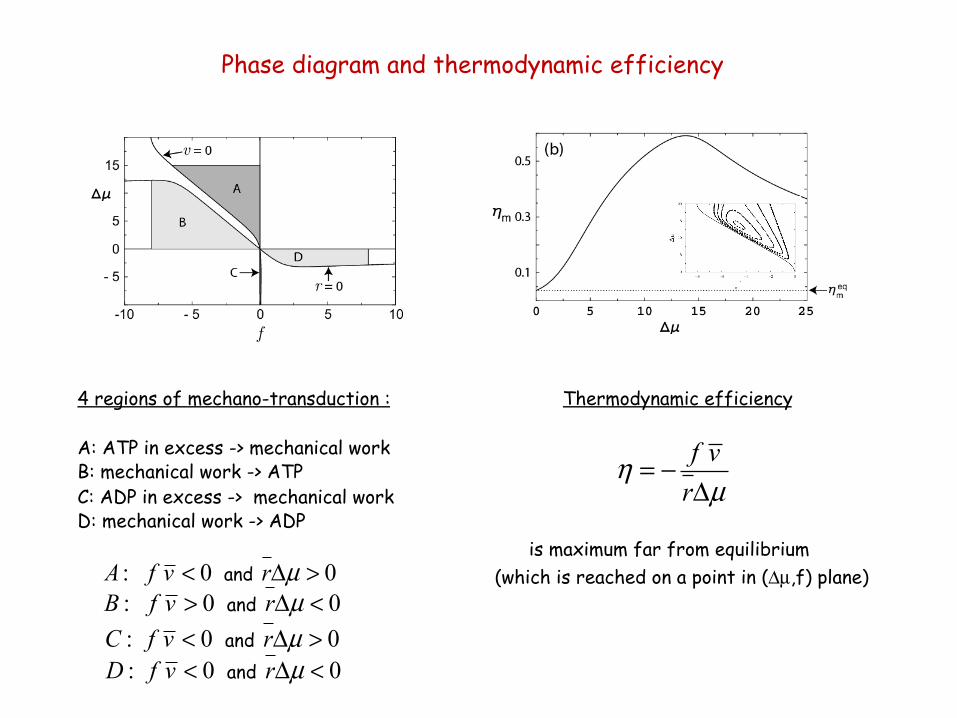
4 regions of mechano-transduction : Thermodynamic efficiency A: ATP in excess -> mechanical work B: mechanical work -> ATP C: ADP in excess -> mechanical work D: mechanical work -> ADP is maximum far from equilibrium (which is reached on a point in (Dµ,f) plane)

Phase diagram and thermodynamic efficiency

: 0 0A f v r µ< Δ >and : 0 0B f v r µ> Δ <and : 0 0C f v r µ< Δ >and : 0 0D f v r µ< Δ <and

f vr

ηµ

= −Δ

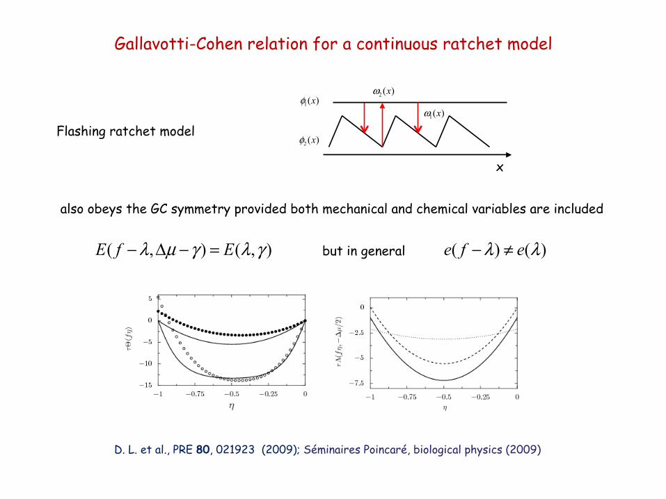
D. L. et al., PRE 80, 021923 (2009); Séminaires Poincaré, biological physics (2009)

Flashing ratchet model also obeys the GC symmetry provided both mechanical and chemical variables are included

( , ) ( , )E f Eλ µ γ λ γ− Δ − = but in general ( ) ( )e f eλ λ− ≠

x

1( )xφ

2 ( )xφ

1( )xω

2 ( )xω

Gallavotti-Cohen relation for a continuous ratchet model

Modified fluctuation-dissipation theorems out of equilibrium

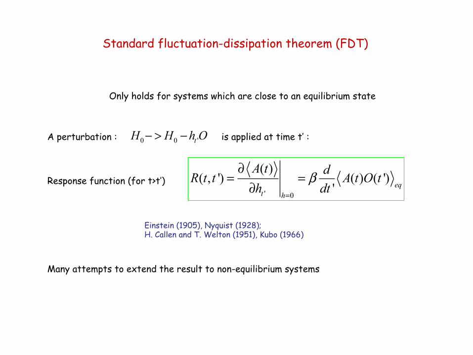
Standard fluctuation-dissipation theorem (FDT)

A perturbation : is applied at time t’ : Response function (for t>t’) Many attempts to extend the result to non-equilibrium systems

0 0 '− > − tH H h O

' 0

( )( , ') ( ) ( ')

'β

=

∂= =

∂ eqt h

A t dR t t A t O th dt

Einstein (1905), Nyquist (1928); H. Callen and T. Welton (1951), Kubo (1966)

Only holds for systems which are close to an equilibrium state

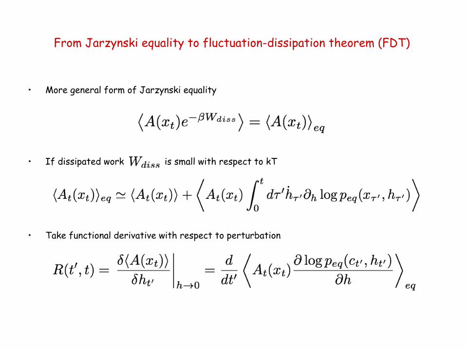
•  More general form of Jarzynski equality

•  If dissipated work is small with respect to kT

•  Take functional derivative with respect to perturbation

From Jarzynski equality to fluctuation-dissipation theorem (FDT)

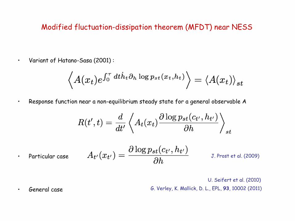
•  Variant of Hatano-Sasa (2001) :

•  Response function near a non-equilibrium steady state for a general observable A

•  Particular case

•  General case

Modified fluctuation-dissipation theorem (MFDT) near NESS

J. Prost et al. (2009)

U. Seifert et al. (2010) G. Verley, K. Mallick, D. L., EPL, 93, 10002 (2011)

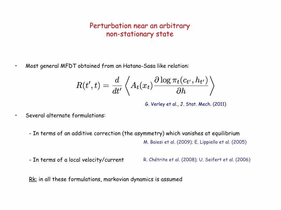
•  Most general MFDT obtained from an Hatano-Sasa like relation:

•  Several alternate formulations:

G. Verley et al., J. Stat. Mech. (2011)

Perturbation near an arbitrary non-stationary state

- In terms of an additive correction (the asymmetry) which vanishes at equilibrium

- In terms of a local velocity/current Rk: in all these formulations, markovian dynamics is assumed

M. Baiesi et al. (2009); E. Lippiello et al. (2005)

R. Chétrite et al. (2008); U. Seifert et al. (2006)

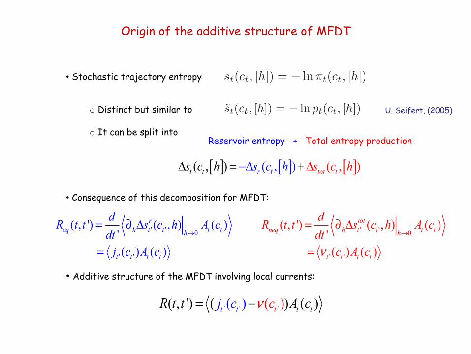
•  Stochastic trajectory entropy

o  Distinct but similar to

o  It can be split into

•  Consequence of this decomposition for MFDT:

•  Additive structure of the MFDT involving local currents:

[ ] [ ] [ ]( , ) ) (, )( ,Δ = −Δ Δ+r t tot tt ts c sh cc h s h

Origin of the additive structure of MFDT

Reservoir entropy +

Total entropy production

' ' 0

' '

( , ') ( , ) ( )'( ) ( )

→= ∂ Δ

=

req h t t t th

t t t t

dR t t s c h A cdtj c A c

' ' 0

' '

( , ') ( , ) ( )'( ) ( )ν

→= ∂ Δ

=

totneq h t t t th

t t t t

dR t t s c h A cdt

c A c

' ' '( )( , ') ( ) () )(ν= −t t tt tR t t Aj cc c

U. Seifert, (2005) s̃t(ct, [h]) = � ln pt(ct, [h])

st(ct, [h]) = � ln⇡t(ct, [h])

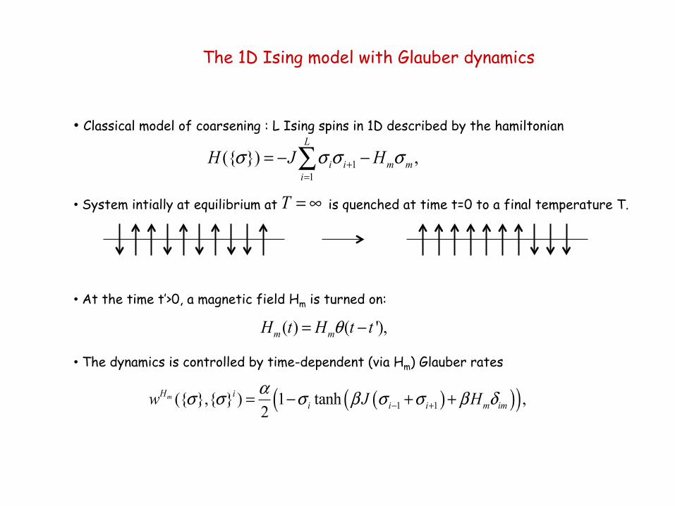
The 1D Ising model with Glauber dynamics

•  Classical model of coarsening : L Ising spins in 1D described by the hamiltonian

•  System intially at equilibrium at is quenched at time t=0 to a final temperature T.

•  At the time t’>0, a magnetic field Hm is turned on:

•  The dynamics is controlled by time-dependent (via Hm) Glauber rates

11

({ }) ,σ σ σ σ+=

= − −∑L

i i m mi

H J H

( )( )( )1 1({ },{ } ) 1 tanh ,2ασ σ σ β σ σ β δ− += − + +mH i

i i i m imw J H

( ) ( '),θ= −m mH t H t t

=∞T

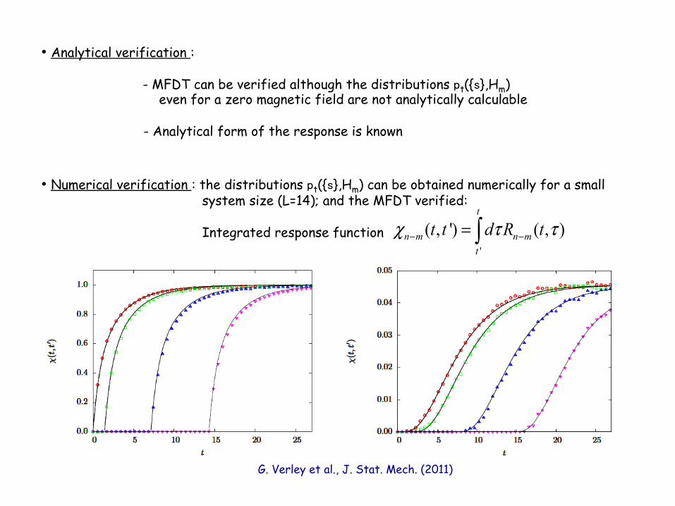
•  Analytical verification :

- MFDT can be verified although the distributions pt({s},Hm) even for a zero magnetic field are not analytically calculable - Analytical form of the response is known •  Numerical verification : the distributions pt({s},Hm) can be obtained numerically for a small system size (L=14); and the MFDT verified:

Integrated response function

'

( , ') ( , )χ τ τ− −= ∫t

n m n mt

t t d R t

G. Verley et al., J. Stat. Mech. (2011)

Fluctuation theorems for equilibrium systems

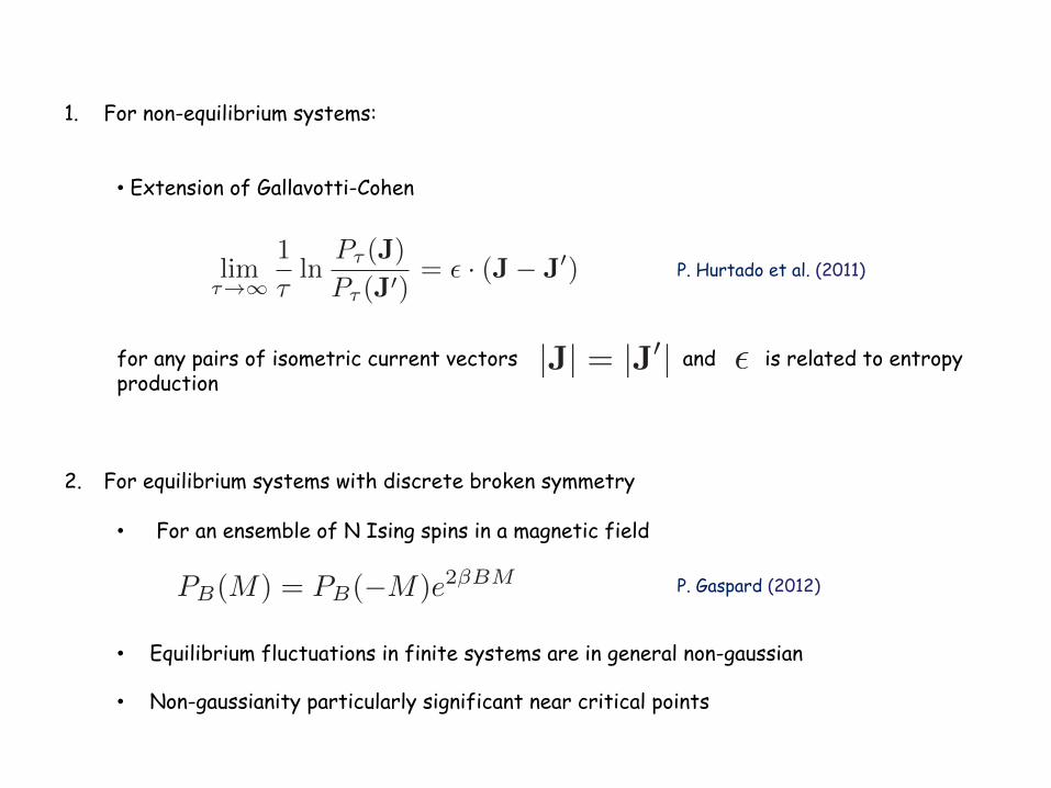
1.  For non-equilibrium systems:

•  Extension of Gallavotti-Cohen for any pairs of isometric current vectors and is related to entropy production

2.  For equilibrium systems with discrete broken symmetry

•  For an ensemble of N Ising spins in a magnetic field

•  Equilibrium fluctuations in finite systems are in general non-gaussian

•  Non-gaussianity particularly significant near critical points

lim⌧!1

1

⌧ln

P⌧ (J)

P⌧ (J0)= ✏ · (J� J0) P. Hurtado et al. (2011)

|J| = |J0| ✏

PB(M) = PB(�M)e2�BM P. Gaspard (2012)

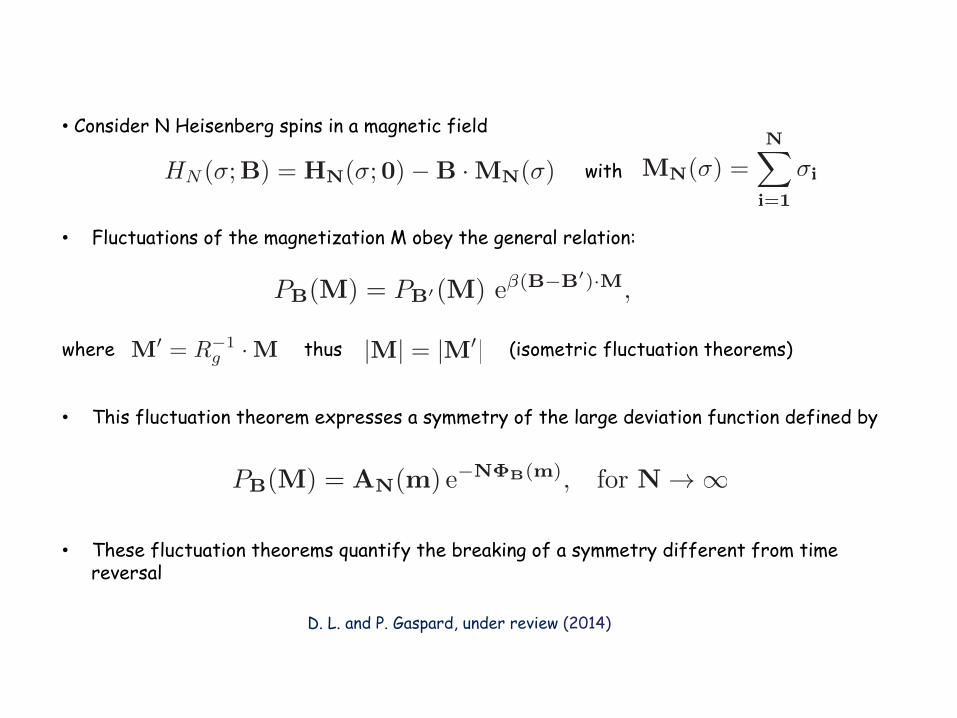
•  Consider N Heisenberg spins in a magnetic field

with •  Fluctuations of the magnetization M obey the general relation: where thus (isometric fluctuation theorems) •  This fluctuation theorem expresses a symmetry of the large deviation function defined by

•  These fluctuation theorems quantify the breaking of a symmetry different from time reversal

PB(M) = PB0(M) e�(B�B0)·M,

PB(M) = AN(m) e

�N�B(m), for N ! 1

HN (�;B) = HN(�;0)�B ·MN(�) MN(�) =NX

i=1

�i

M0 = R�1g ·M |M| = |M0|

D. L. and P. Gaspard, under review (2014)

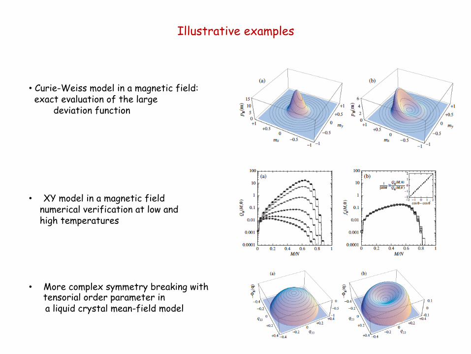
Illustrative examples

•  Curie-Weiss model in a magnetic field: exact evaluation of the large deviation function

•  XY model in a magnetic field numerical verification at low and high temperatures

•  More complex symmetry breaking with tensorial order parameter in

a liquid crystal mean-field model

Non-invasive estimation of dissipation from trajectory information

Irreversibility as time-reversal symmetry breaking

•  Direct determination of work or heat is difficult for most complex systems

•  Non-equilibrium fluctuations created by irreversible processes have a well-defined arrow of time

•  This arrow of time can be « measured » by comparing the statistics of fluctuations forward and backward in time using the KL divergence

•  This amounts to enforce fluctuation theorems and exploit them to extract a measurement rather than trying to « verify » them

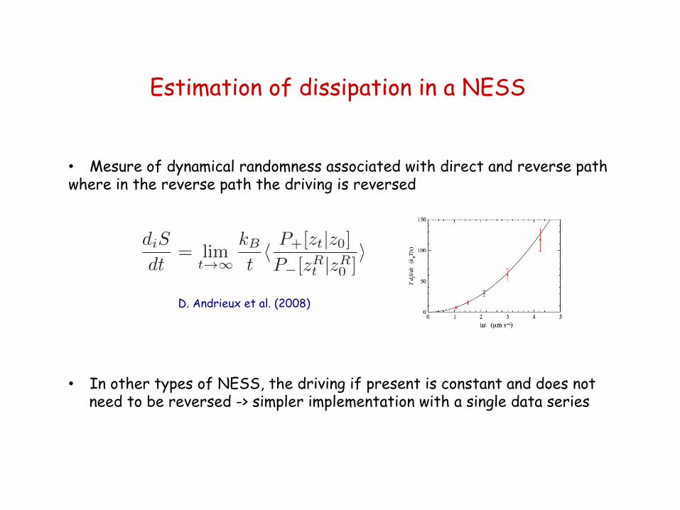
Estimation of dissipation in a NESS

•  Mesure of dynamical randomness associated with direct and reverse path where in the reverse path the driving is reversed

•  In other types of NESS, the driving if present is constant and does not need to be reversed -> simpler implementation with a single data series

diS

dt= lim

t!1

kBth P+[zt|z0]P�[zRt |zR0 ]

i

D. Andrieux et al. (2008)

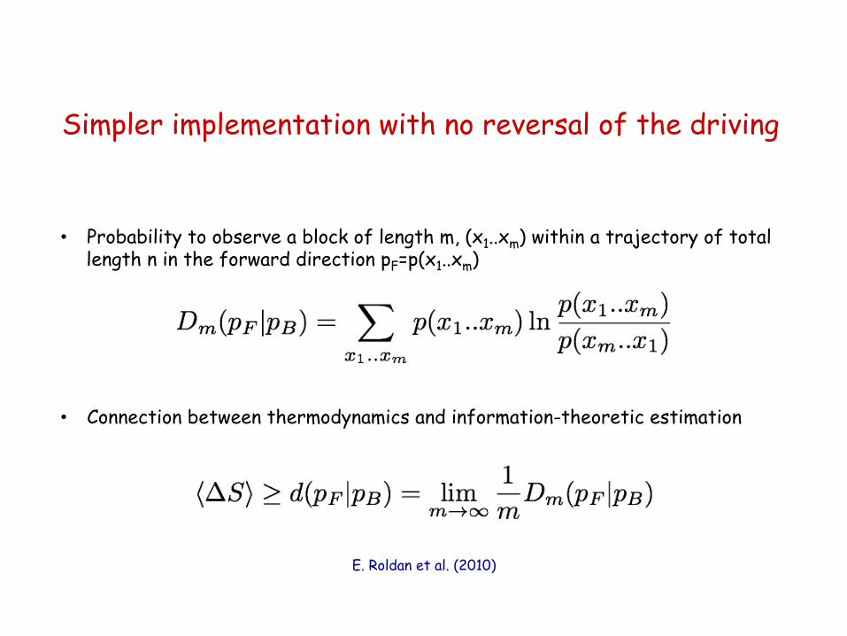
•  Probability to observe a block of length m, (x1..xm) within a trajectory of total

length n in the forward direction pF=p(x1..xm)

•  Connection between thermodynamics and information-theoretic estimation

Simpler implementation with no reversal of the driving

E. Roldan et al. (2010)

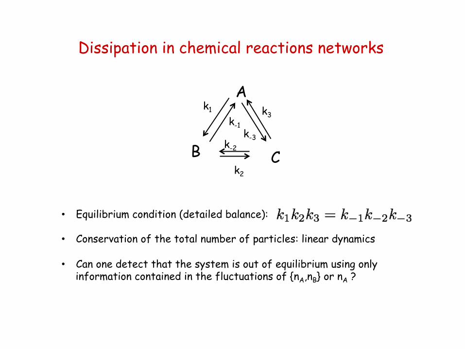
•  Equilibrium condition (detailed balance):

•  Conservation of the total number of particles: linear dynamics

•  Can one detect that the system is out of equilibrium using only

information contained in the fluctuations of {nA,nB} or nA ?

A

B C

k-1

k1 k3

k-3

k2

k-2

Dissipation in chemical reactions networks

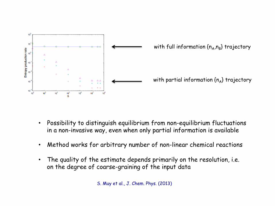
with full information {nA,nB} trajectory

S. Muy et al., J. Chem. Phys. (2013)

with partial information {nA} trajectory

•  Possibility to distinguish equilibrium from non-equilibrium fluctuations

in a non-invasive way, even when only partial information is available

•  Method works for arbitrary number of non-linear chemical reactions

•  The quality of the estimate depends primarily on the resolution, i.e. on the degree of coarse-graining of the input data

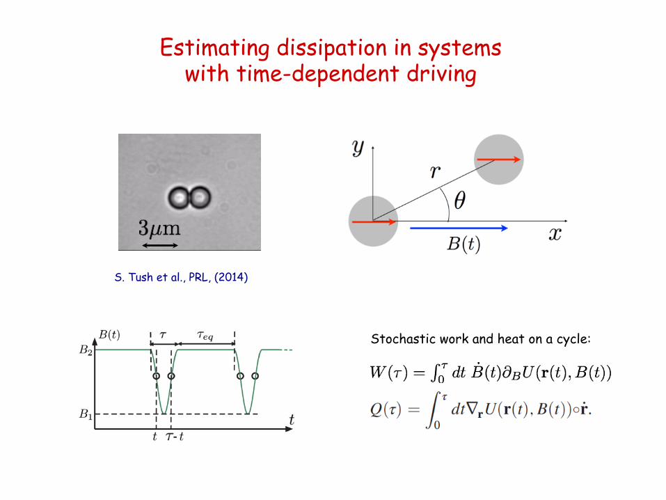
Estimating dissipation in systems with time-dependent driving

S. Tush et al., PRL, (2014)

Stochastic work and heat on a cycle:

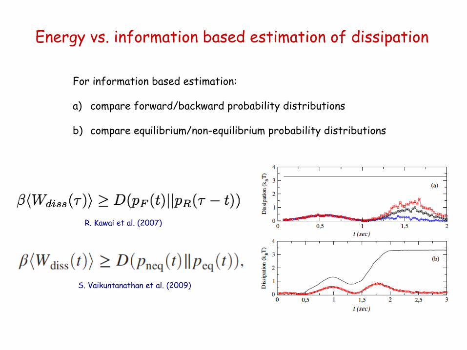
Energy vs. information based estimation of dissipation

R. Kawai et al. (2007)

For information based estimation: a)  compare forward/backward probability distributions

b)  compare equilibrium/non-equilibrium probability distributions

S. Vaikuntanathan et al. (2009)

Acknowledgements  

1.  Fluctuation theorems for systems out of equilibrium K. Mallick, A. Lau 2.  Fluctuations theorems for systems at equilibrium P. Gaspard 3.  Modified fluctuation-dissipation theorems out of equilibrium R. Chétrite, G. Verley 4.  Non-invasive estimation of dissipation from trajectory information

Theory: A. Kundu, G. Verley Experiments with manipulated colloids: S. Tush, J. Baudry