Flows in environmental fluids and porous media

INTERNATIONAL JOURNAL OF ENERGY RESEARCHInt. J. Energy Res. 2003; 27:825–846 (DOI: 10.1002/er.913)

Flows in environmental fluids and porous media

Adrian Bejann,y

Department of Mechanical Engineering and Materials Science Duke University, Durham, NC 27708-0300, USA

SUMMARY

This paper reviews some of the most basic flows that effect the dispersal of heat and mass in environmentalconfigurations. Two important classes of environmental flows are discussed: free turbulent flows (shearlayers, jets, plumes and wakes) and free flows in porous media (plumes, wakes behind concentrated sourcesof heat and mass, plumes, penetrative convection). These flows are ‘free’ from the effect of confiningboundaries. The emphasis is on fundamental mechanisms and the methods (use the simplest first) that havebeen developed for the prediction and description of environmental flows. Copyright# 2003 John Wiley &Sons, Ltd.

KEY WORDS: plumes; jets; shear layers; porous media; penetrative convection; concentrated sources;turbulent; environmental; pulsating fires; stratified flows

1. ENERGY AND THE ENVIRONMENT

Realistic models of energy systems demand the treatment of installations and their flowingsurroundings together, more so when the installations are large and their spheres of impactgreater. This unified treatment is the ultimate objective of the research interface called ‘‘energyand the environment’’. In this article I review the fundamentals of some of the most importanttypes of flows that govern the behaviour of environmental fluids (air, water) and fluid-saturatedporous media.

On the fluid-flow side, the most important class are the free stream turbulent flows}shearlayers, jets, plumes}flows that are free from wall effects because they are situated sufficientlyfar from solid boundaries (Bejan, 1995). We are particularly interested in turbulent flowsbecause the flows that effect the interaction between our installations and their environments arehighly turbulent. They are high Reynolds number flows. The smoke plume swept by the wind inthe wake of an industrial area and the water jets discharged by a city into the river are examplesof how our presence impacts what surrounds us.

Free-stream flows rely on turbulent mixing to diffuse away our refuse and, in this way, tominimize the negative effect that high concentrations of such refuse (heat, species) might have

Copyright # 2003 John Wiley & Sons, Ltd.

nCorrespondence to: Dr. A Bejan, Department of Mechanical Engineering and Materials Science, Duke University,Durham, NC 27708-0300, U.S.A.

yE-mail: [email protected]

on the biosphere. Turbulent mixing is the most effective transport mechanism known: in fact,the occurrence of turbulence in any flow is anticipated on a theoretical basis by the constructalprinciple of maximizing the speed with which the mixed region spreads (Bejan, 2000). Tointroduce the energy engineer to the most basic characteristics of this mechanism is the objectiveof Section 2.

The fundamentals of the modelling of environmental flows through fluid-saturated porousmedia are outlined in Section 3. This field experienced significant growth during the past 2decades, and now is one of the most active in thermal sciences (Nield and Bejan, 1999). Itsdevelopment is comparable with that of classical convection (transport by the flow of a purefluid): governing principles are in place, experimental data continue to stimulate improvementsin the governing principles, and there is an abundance of practical applications. From anenvironmental standpoint, the fundamental aspects that are covered in Section 3 are relevant tounderstanding the spreading of contaminated fluids through the ground, the leakage of heatthrough the walls of buildings, and the flow of geothermal fluids through the earth’s porouscrust.

2. FREE TURBULENT FLOWS

2.1. Free shear layers

The simplest turbulent mixing configuration is shown in Figure 1. A free shear layer forms in thevicinity of the interface between a moving fluid region and a region filled by stationary fluid. Forexample, two shear layers form immediately downstream of a slit (a two-dimensional nozzle).The shear-layer region sketched in Figure 1 refers to the time-averaged flow. The instantaneousflow is dominated by a ladder of large and growing eddies, so large that their diameters definethe thickness of the shear layer.

One key question in the study of environmental flows is how fast and how far the mixingregion spreads. In a free shear layer then, a key unknown is the thickness of the shear layer}thetransversal dimension D, as a function of the longitudinal distance x. Related to this question ishow the mixing region is influenced by the flow discontinuity (e.g. industrial discharge) thatdrives the mixing. In Figure 1, the driving effect is provided by the velocity and temperaturediscrepancies between the nozzle conditions (U0, T0) and the conditions in the stagnant fluidzone (U1, T1).

The mixing phenomenon has two parts, which in the absence of significant body forces aredecoupled: momentum transport, or the smoothing of the velocity distribution, and energytransport, or the smoothing of the temperature distribution. Starting with the momentummixing, the time-averaged equations for mass and momentum conservation in the (x, y) framedefined in Figure 1 are (Bejan, 1995)

@ %uu

@xþ

@%vv

@y¼ 0 ð1Þ

%uu@ %uu

@xþ %vv

@ %uu

@y¼ �

1

rd %PP

dxþ

@

@ynþ eMð Þ

@ %uu

@y

� �ð2Þ

The symbols appearing in these equations and the rest of the paper are defined in nomenclature.Overbars indicate time-averaged quantities. Equation (2) is of the boundary layer type: it applies

Copyright # 2003 John Wiley & Sons, Ltd. Int. J. Energy Res. 2003; 27:825–846

A. BEJAN826

inside the shear layer region x�D provided that region is slender, D � x: The unknowns( %uu; %vv; %PP; eM) exceed the number of equations. Three assumptions define the classical route ofclosing this and the similar problems reviewed in this section:

(a) The longitudinal pressure gradient inside the mixing region d %PP=dx is the same as on theoutside, dP1=dx ¼ 0: This is a consequence of the slenderness of the mixing region.

(b) The molecular kinematic diffusivity n is neglected in favour of the eddy diffusivity eM inEquation (2). This is true sufficiently downstream the shear layer, starting with the ‘virtualorigin’’ x ¼ 0 located in the vicinity of the transition from laminar shear to turbulent shear.

(c) The empirical observation that in an actual flow D appears to be proportional to x,

D=x � constant ð3Þ

leads to a model}a formula}for eM. Specifically, Equation (2) demands the equivalence ofscales U 2

0 =x � eMU0=D2; which combined with Equation (3) yields

eM � U0x ð4Þ

Prandtl’s (1969) alternative was to derive Equation (4) by combining observation (3) from hismixing length model (Schlichting, 1960; Bejan, 1995). In the buckling theory of turbulent flowEquation (4) is theoretical, not empirical, because Equation (3) is deduced, not assumed (Bejan,1995, Chapter 6, pp. 376–378): the predicted form of Equation (3) is D=x � tanðD=3lBÞ ¼ 0:19;where lB is the buckling wavelength at the location x where the layer thickness is D.

Figure 1. The development of two free shear layers on both sides of a two-dimensional jet.


FLOWS IN ENVIRONMENTAL FLUIDS AND POROUS MEDIA 827

Simplified according to assumptions (a)–(c), Equations (1) and (2) can be solved numericallyin similarity formulation to obtain the flow field ( %uu; %vv) subject to the far-field conditions %uu ¼ U0

as y ! 1 and %uu ¼ %vv ¼ 0 as y ! �1 (Prandtl, 1969; Schlichting, 1960). In the similarityformulation Equation (4) assumes the form eM ¼ U0x=ð4s2Þ; where s is an empirical constant. Acurve fit to the numerical solution is the longitudinal velocity profile (e.g. Bejan, 1995)

%uu ¼ 12U0 1þ erf sy=x

� �� ð5Þ

for which the constant has been determined from measurements, s ffi 13:5: If we takeerf(1.16)ffi0.9 to represent the edge of the time-averaged shear layer (y � D=2), then the error-function argument sðD=2Þ=x ¼ 1:16 means that D=x � 0:17; which is in agreement with thetheoretical expression listed under Equation (4).

The thermal mixing between the two fluid regions (T0; T1) of Figure 1 is accounted for by thetime-averaged energy equation

%uu@ %TT

@xþ %vv

@ %TT

@y¼ eH

@2 %TT

@x2ð6Þ

where eH is the thermal eddy diffusivity already modelled in accordance with assumptions(b) and (c). The simplest approach is to use the hypothesis that the turbulent Prandtl numberPrt ¼ eM=eHffi1; so that the %TTðx; yÞ problem becomes analogous to the %uuðx; yÞ problem reviewedalready, and the %TT solution can be curve fitted in the same way as Equation (5):

%TT� T1T0 � T1

ffi%uu

U0ffi

1

21þ erf s

yx

� �h ið7Þ

These velocity and temperature distributions indicate that the most intense rates of momentumand heat transport occur across the initial plane of separation, y ¼ 0: For example, the flow ofenergy (enthalpy) across the y ¼ 0 plane occurs at the rate q00y¼0 ¼ rcpeHð@ %TT=@yÞy¼0; whichcombined with Equation (7), eH ffi eM; and eM ¼ U0x=ð4s2Þ; becomes

Sty¼0 ¼q00y¼0= T0 � T1ð Þ

rcpU0¼

1

4sp1=2ffi 0:01 ð8Þ

In conclusion, the transport rate across the separation plane x-independent, and the associatedStanton number (Equation (8)) is a constant.

2.2. Jets

The time-averaged mixing and growth of a turbulent two-dimensional jet region is summarizedby a treatment similar to that of the two-dimensional shear layer (Section 2.1). Consider theconfiguration of Figure 2: a jet of velocity U0 and temperature T0 is injected through a slit ofspacing D0 into a stagnant isothermal reservoir (T1) containing the same fluid as the jet. Theinitial mixing between the U0 and U1 ¼ 0 regions is ruled by the free shear layer phenomenon(Figure 1). The two shear layers grow linearly and merge downstream at a distance proportionalto the nozzle dimension D0. In the shear layer section the centreline velocity is nearly equal toU0, and is independent of x. Downstream of the merger of the two shear layers the streamproceeds as a jet with a centreline velocity %uuc that decreases monotonically in the x direction.The following description applies only to the downstream jet region, again, based on theassumption that this region is slender: D � x; where DðxÞ is the transversal length scale of the jetregion.


A. BEJAN828

The analytical description of the jet velocity distribution is based on the mass and momentumequations (1) and (2) coupled with assumptions (a)–(c). In particular, (c) is justified bymeasurements that show that D is proportional to x, or is deduced from theory (Bejan, 1995,Chapters 6 and 9). Defined by the D/x=constant proportionality, the point at x ¼ 0 representsthe virtual origin of the jet region (Figure 2). After assumptions (a)–(c), Equation (2) assumes asimpler form involving the eddy diffusivity model

eM ¼1

4g2%uucx ð9Þ

where the constant g is determined from experiments or theory. Jet flows have the additionalproperty that their longitudinal momentum is conserved. Integrating the momentum equationall the way across the jet, in the plane x=constant, we find the ‘jet strength’ constraintZ 1

�1%uu2 dy ¼ U 2

0D0 ð10Þ

where D0 is the diameter of the round nozzle. This represents the scaling %uu2cD � U20D0: Defining

x0 as the distance from the nozzle exit to the virtual origin of the jet, x=x0 ¼ D=D0; constraint(10) requires

%uuc

U0¼

xx0

�1=2

ð11Þ

The centerline velocity decays as x�1/2, as a consequence of the linear growth (D � x) and thestrength constraint (10). This behaviour is the basis for the similarity solution for %uuðx; yÞ (for

Figure 2. The large-scale instantaneous (buckled) structure of a two-dimensional turbulent jet, and theconstant-angle shape of the time-averaged jet flow region (Bejan, 1995).



details see Bejan, 1995),

%uu ¼ U0xx0

�1=2

ð1� tanh2ZÞ ð12Þ

where Z ¼ gy=x: Substituted into constraint (10), the %uu solution pinpoints the value of x0,namely x0 ¼ ð3=4ÞgD0: The empirically determined constant (g ffi 7:67) is of the same order(about half) as the constant s determined for free shear layers, and stresses the universality ofthe theoretical linear growth of all free turbulent flows (Table I).

The temperature distribution in the jet region follows closely the velocity distribution. This isto be expected, because the same large-scale eddies (D size) rule the velocity and thermal mixing.Experimentally it is found that the temperature distribution is fitted well by

%TT� T1%TTc � T1

¼%uu

%uuc

0:5

ð13Þ

The centreline excess temperature ð %TTc � T1Þ decreases as x�1/2, in the same manner as %uuc:Curvefit (13) shows that the temperature profile is somewhat broader than the %uu profile at thesame x.

Round turbulent jets have been treated similarly. The momentum eddy diffusivityscales as eM � %uucx; and the jet strength constraint requires a faster decay of thecentreline velocity, %uuc � x�1: In place of the similarity solution (Bejan, 1995, p. 384),more commonly used in environmental engineering is the Gaussian form (Fischer et al.,1979),

%uu ¼ %uucexp �ðr=bÞ2� �

ð14Þ

Experiments with water jets indicate that the length scale (b) in the radial direction (r) isproportional to the jet length x,

b=x ¼ 0:107� 0:003 ð15Þ

which transforms Equation (14) into %uu= %uuc ¼ exp½�ð9:35 r=xÞ2�: The corresponding jet strengthconstraint is %uuc ¼ 7:46 K1=2=x; where the conserved longitudinal momentum (K) is

K ¼ 2pZ 1

0

%uu2r dr ¼p4U2

0D20 ð16Þ

Table I. The longitudinal variation (x) of the time-averaged scales of free turbulent flows (Bejan, 1995).

Configuration D %vvc ð %TTc � T1Þ

Shear layersTwo-dimensional x x0 x0

JetsAxisymmetric x x�1 x�1

Two-dimensional x x�1/2 x�1/2

PlumesAxisymmetric x x�1/3 x�5/3

Two-dimensional x x0 x�1


A. BEJAN830

The temperature distribution is again closely related to the velocity distribution. Thecorresponding Gaussian profile is (Fischer et al., 1979)

%TT� T1 ¼ %TTc � T1� �

exp � r=bT� �2h i

ð17Þ

where the effective radius of the thermal jet is averaged based on measurements,

bT=x ¼ 0:127� 0:004 ð18Þ

Comparing Equations (18) and (15) we note that the temperature profile is slightly broader thanthe velocity profile, bT=b ffi 1:2: The axial decay of the centreline excess temperature is dictatedby the conservation of energy in any constant-x plane,

2pZ 1

0

rcP %uu %TT� T1� �

r dr ¼ rcPU0 T0 � T1ð Þp4D2

0 ð19Þ

where the right-hand side is the enthalpy flow rate through the plane of the round nozzle ofdiameter D0, velocity U0, and temperature T0. Equations (17)–(19) yield

%TTc � T1� �

= T0 � T1ð Þ ¼ 5:65D0=x ð20Þ

The centreline excess temperature decreases as x�1. Taken together, Equations (17) and (20)describe the extent to which the thermal jet has spread into the isothermal and stagnantreservoir.

When a jet is discharged horizontally into a density stratified (or thermally stratified)reservoir, it becomes turbulent only if the stratification is sufficiently weak. Consider the densitystratification rðyÞ ¼ r02by; where y is the vertical direction, and b ¼ �dr=dy > 0 is the densitygradient (the degree of stratification). The density gradient b should not be confused with theradial length scale appearing in Equation (14). The jet, as any other stream, has the property tobuckle with the longitudinal length scale lB (buckling wavelength) such that lB/D�2, where Dis the local transversal dimension of the stream. The length lB is theoretical. A back of theenvelope analysis shows that a direct consequence of the geometric similarity rule lB/D�2 is thecondition for transition to a turbulent jet in a stratified reservoir,

gb

r V =D� �2 9 1

4ð21Þ

The group on the left-hand side is also known as the Richardson number, Ri, where g is thegravitational acceleration. Equation (21) has also been derived based on a much more extensivehydrodynamic stability analysis (Jaluria, 1980).

The buckling wavelength scaling lB � 2D has also been used to correlate all the observationsof transition to turbulence (Bejan, 1995, Table 6.2). The universal dimensionless condition fortransition to turbulent flow is

VDn

� Oð102Þ ð22Þ

where V and D are the local scales of the longitudinal velocity and transversal dimension of theflow. For example, the laminar-turbulent shear layer transition of Figure 1 is governed byEquation (22).



2.3. Plumes

Plumes are similar to jets, except that they are driven by buoyancy, not by the momentumimparted by the flow exiting the nozzle. Consider Figure 3: heated fluid rises above a point heatsource of power q(W). Attached to the time-averaged mixing region is the cylindrical system(y, r), such that y ¼ 0 marks the virtual origin of the mixing region. Again, the classicaltreatment is based on the observation that the mixing region is cone shaped, D=y ¼ constant:

The similarity solution is based on the steps outlined in Section 2.1. More frequently used isthe integral-method solution (Turner, 1973, Gebhart et al., 1988), in which the eM model(assumption (c) of Section 2.1) is replaced by the ‘‘entrainment hypothesis’’ that at the edge ofthe mixing region (r ! 1) the group r %uu is of the same order of magnitude as the group b%vvc;where %uu; b and %vvc are the horizontal (entrainment) velocity, radial length scale of the mixingcone, and centreline velocity. This assumption is consistent with the geometric view that themixing is dominated by the largest eddies (Figure 3), the length scale of which is b. Since %uu is

Figure 3. The buckled shape of a turbulent plume above a concentrated heat source, and the funnel shapeof the time-averaged mixing region (Bejan, 1995).


A. BEJAN832

negative, the entrainment hypothesis is the statement

r %uuð Þ1¼ � #aab%vvc ð23Þ

where #aa is determined empirically, #aa ¼ 0:12: Next, instead of the momentum integral (10), wewrite that the plume is the result of the balance between buoyancy and the rate of increase invertical momentum,

d

dy

Z 1

0

%vv2r dr ¼ gbZ 1

0

ð %TT� T1Þr dr ð24Þ

Similarly, in place of the energy conservation integral (19) we have the plume strength integral

q ¼ 2prcP

Z 1

0

%vvð %TT� T1Þr dr ð25Þ

Finally, Gaussian profiles are assumed for the vertical velocity and excess temperatureprofiles,

%vv ¼ %vvcexp � r=b� �2h i

ð26Þ

%TT� T1 ¼ %TTc � T1� �

exp � r=bT� �2h i

ð27Þ

The integral solution resulting from the integral analysis is (Bejan, 1995)

b ¼ ð6=5Þ#aay ð28Þ

%vvc ¼25qgb

24p#aa2rcPy1þ

b2Tb2

� �1=3ð29Þ

%TTc � T1 ¼ 0:685#aa�4=3 gbð Þ�1=3 1þ b=bT� �2h i

1þ bT=b� �2h i�1=3

q=prcP� �2=3

y�5=3 ð30Þ

This solution shows that in a round plume the centreline velocity decays as y�1/3, and thecentreline excess temperature decays as y�5/3. The corresponding features of the two-dimensional (wedge shaped) turbulent plume (cf. Bejan, 1995, Problem 9.3) are summarizedin Table I.

The analysis summarized in this section can be extended to the more general case where theinitial section of the plume is a forced jet, defined by a nozzle of known flow rate ð%vvcb2Þy¼0 andknown momentum strength ð%vv2cb

2Þy¼0: Given enough time, that is, above a certain height, thestrength of the buoyant jet becomes dominated by the effect of buoyancy, and the behaviour ofthe buoyant jet becomes similar to that of the simple plume. The height y above which the initialjet becomes a plume can be estimated by comparing the local (y) strength of the plume [%vv2cb

2;Equations (28)–(30)] with the initial jet strength, ð%vv2cb

2Þy¼0: These combinations of jet and plumeeffects are covered in more detail in Jaluria (1980).

As a reminder that all the flows covered in this section have been subjected to time averaging,we note that the intermittency of turbulent flow is most evident in how plumes pulsate above theheat sources that generate them. Fires pulsate with a frequency fv that scales as D

�1/2, where D isthe fire base length scale

f 2v ffi

2:3 m=s2

Dð31Þ



To predict this frequency was a problem proposed by Prof. P. J. Pagni of the University ofCalifornia, Berkeley, in the ASME forum on Some Unanswered Questions in Fluid Mechanics(Pagni, 1989). He noted that ‘it has been known for 20 years that fires pulsate with a regularfrequency, releasing large annular vortices (coherent structures) from their bases. What is notknown is why Equation (31) describes the shedding frequency of pool-flame oscillation overmore than three orders of magnitude of the flame base diameter, from D � 0:03 to 60m?’

The explanation for Equation (31) lies in the geometric similarity of the buckled (meandering)plume shape, lB=D � 2; which also accounted for the Richardson number criterion (21) and thelaminar-turbulent flow transition criterion (22). Near its base, the plume exhibits the lB=Dscaling law, e.g. Figure 3. In another back of the envelope analysis, Bejan (1991, 1995) showedthat Equation (31) follows from combining lB=D � 2 with the well-known description of aninviscid plume that accelerates upward. Combining this with the transition criterion (22) yieldsthe prediction that fire plumes will oscillate only if their bases are large enough such thatD90:02 m: This agrees well with Pagni’s observation that oscillations occur above D � 0:03 m:The theory, however, contributes the thought that oscillations will be present in pool fires withbase diameters even larger than 60m, i.e. beyond the range noted by Pagni.

2.4. Thermal wakes behind concentrated sources

An even simpler way to model the dispersion of thermal pollution in the wake of a concentratedheat source is shown in Figure 4. Consider a line heat source of power q0(W/m) normal to atime-averaged uniform stream ð %UU1; %TT1Þ populated throughout by eddies that have the samecharacteristic size and peripheral speed. This type of turbulence can be created in the laboratory,immediately behind a turbulence-generating grid installed normal to the flow in a wind tunnel.In nature, grid-generated turbulence is no more than an approximate model for the eddytransport capability of large streams that bathe concentrated sources of heat or mass (e.g. theatmospheric boundary layer and the mainstream section of a river). The eddy population insuch streams is the result of earlier (upstream) stream–wall and stream–stream interactions.

Figure 4. The development of a thermal wake behind a line heat source perpendicular to a uniform streamwith grid-generated turbulence (Bejan, 1995).


A. BEJAN834

The energy equation applicable to this situation is,

%UU1@ %TT

@x¼ eH

@2 %TT

@y2ð32Þ

has already been simplified based on the following assumptions: (d) The thermal eddy diffusivityis much greater than the molecular diffusivity, eHa; (e) The thermal wake region is slender; (f)The eddy diffusivity eH is not a function of either y or x; the value of this constant, assumedknown, is controlled by the mechanism that generates turbulence in the %UU1 stream. The scaleanalysis of the energy equation shows that the thermal wake thickness scales as ðeHx= %UU1Þ1=2:The scale analysis of the enthalpy conservation constraint

q0 ¼ rcP

Z 1

�1

%UU1ð %TT� %TT1Þ dy ð33Þ

shows that the centreline-to-ambient temperature difference ð %TTc � %TT1Þ scales as ðq0=rcP Þ �ð %UU1eHxÞ

�1=2: The similarity solution recommended by these results is Bejan (1995)

%TT x; yð Þ � %TT1� � %UU1eHx

� �1=2q0=rcP

¼1

2p1=2exp �

Z2

4

ð34Þ

Z ¼ y %UU1=eHx� �1=2

ð35Þ

In conclusion, the time-averaged temperature field behind the line source has a Gaussian profilethe span of which increases as x1/2. The centreline temperature difference ð %TTðx; ; 0Þ � %TT1Þdecreases as x�1/2 in the flow direction. The temperature field is known if the eddy diffusivity eHassociated with the uniform turbulence is known; in fact, the above solution can be combinedwith actual measurements of %TTðx; yÞ in order to calculate the eH value of a certain population ofeddies produced by a certain laboratory technique.

The thermal wake behind a point source immersed in grid-generated turbulence can beanalysed according to the same model. The temperature field is given by (cf. in Bejan, 1995,Problem 9.4)

%TTðx; yÞ � %TT1 ¼q

4prcP eHxexp �

%UU1r2

4eHx

ð36Þ

where q(W) is the strength of the point source and r is the radial distance measured away fromthe wake centreline.

2.5. Mass transfer

The analogy between mass transfer and heat transfer makes many turbulent thermal mixingresults convertible into formulas for accounting for the spreading of a chemical species. In placeof the energy equation (6), the conservation of species in the time-averaged flow field isdescribed by

%uu@ %CC

@xþ %vv

@ %CC

@y¼

@

@yDþ emð Þ

@ %CC

@y

" #ð37Þ

where %CC (kg speciesm�3) is the time-averaged volumetric concentration, D is the molecular massdiffusivity, and em is the mass eddy diffusivity. A useful simplification that makes the analogy



even more transparent is the hypothesis that the turbulent Schmidt number (eM/em) isapproximately equal to 1.

For example, by analogy with Equations (17) and (18), the turbulent mixing zone created bythe discharge of a round jet of concentration C0 into a stagnant reservoir of concentration C1

has a mixing region described by

%CC� C1

%CCc � C1ffi exp �

r0:127x

� �2� �

ð38Þ

The centreline concentration %CCc is related to the concentration C0 in the nozzle of radius r0 byinvoking the conservation of species in every constant-x plane,Z 1

0

%uu %CC� C1� �

r dr ¼ U0 C0 � C1ð Þr20=2 ð39Þ

Another example is the concentration downstream from a point mass source of strength’mm(kg s�1) bathed by a turbulent stream with uniform time-averaged velocity %UU1 and uniform em(grid-generated turbulence, Figure 4),

%CC� C1 ¼’mm

4pemxexp �

r2 %UU1

4emx

ð40Þ

The concentration distribution in the wake of a line source of size ’mm(kg s�1m�1) is described by

%CC� C1 ¼’mm0

4p %UU1emx� �1=2 exp �

y2 %UU1

4emx

ð41Þ

where y is measured transversally, away from the plane of symmetry of the wake. Furtherexamples of turbulent mixing in environmental mass convection are covered in Fischer et al.(1979).

3. FREE FLOWS IN POROUS MEDIA

3.1. Fundamentals

In this section we turn our attention to several classes of environmental flows through saturatedporous media. These flows have features in common with some of the examples treated inSection 2. The most important is that they are ‘‘free’’ from interaction with solid boundaries. Wewill review the main results that are available for calculating the rate of spreading or mixingthrough wakes, plumes and penetrative convection. The flow description is based on volume-averaging the relevant properties (velocity, temperature) of the porous medium with fluid in itspores. The fluid is single phase. It is assumed that the smallest (infinitesimal-like) volume forwhich the following description is valid meets the condition that it is a representative elementaryvolume (r.e.v., Bear, 1972; Greenkorn, 1983; Nield and Bejan, 1999), which means that itslength scale is at least one order of magnitude greater than the pore length scale. The r.e.v.assumption is particularly well suited for the description of environmental flows such as waterseepage through soil or sand. It is further assumed that the fluid saturated porous medium ishomogeneous and isotropic.


A. BEJAN836

Mass conservation is accounted for by the equation

f@r@t

þr rvð Þ ¼ 0 ð42Þ

where f is the porosity or void fraction, r is the fluid density and v(u, v, w) is the volume-averaged velocity vector. For momentum conservation, the simplest and most applicable is theDarcy flow model,

v ¼K

m�rP þ rgð Þ ð43Þ

where m, P, K and g are the fluid viscosity, pressure, porous medium permeability, andgravitational acceleration vector. In the following examples the porous medium is assumedhomogeneous and isotropic such as K is constant. The permeability K has the units (m2), and isusually determined empirically. For example, the permeability of a column of packed spheres iscorrelated by K ¼ d2f3=½180ð1� fÞ2�; in which d is the sphere diameter. The Darcy flow modelis valid when the pore Reynolds number uK1=2=n"O (10), where u is the scale of the volume-averaged velocity. Faster flows require descriptions based on extended Darcy models, forexample, the Forchheimer and Brinkman models. These extensions are detailed in Nield andBejan (1999).

The conservation of energy in volume-averaged flow is governed by the equation

s@T@t

þ v rT ¼ ar2T ð44Þ

where s is the capacity ratio

s ¼ fþ ð1� fÞðrcÞs=ðrcP Þf ð45Þ

and (rc)s and (rcP)f are the heat capacities of the solid (matrix) and fluid present in the r.e.v. Thethermal diffusivity a ¼ k=ðrcP Þf is based on the effective thermal conductivity of the porousmatrix when its pores are filled with fluid. Equation (44) holds for porous media withoutvolumetric heat generation. The temperature T represents the local temperature of the solid andfluid at the same point (r.e.v.), in other words, it is assumed that the solid matrix is locally inthermal equilibrium with the fluid.

3.2. Concentrated heat sources in uniform flow

Consider the uniform flow (u) through a porous medium (Figure 5) and the development ofthermal wakes downstream of concentrated sources of heat. These configurations are analogousto the thermal wake of Figure 4, except that instead of eddy mixing in Figure 5 the heating effectis dispersed by thermal diffusion through the porous medium. This analogy makes the problemequivalent to that of Section 2.4, therefore in this section we review only the results.

The temperature field behind a point heat source (Figure 5(a)) of strength q buried in a fluidsaturated porous medium is, cf. Equation (40),

T � T1 ¼q

4pkxexp �

ur2

4ax

ð46Þ

This result is valid in the limit where convection overwhelms diffusion as a longitudinal heattransfer mechanism in the wake, i.e. where ux=a 1:



The thermal wake behind a line heat source perpendicular to a uniform volume-averaged flow(u, T1) is sketched in Figure 5(b). If the source strength is q0, the two-dimensional temperaturedistribution T(x, y) is analogous to Equation (41),

T � T1 ¼q0

rcp� �

f4puaxð Þ1=2

exp �uy2

4ax

ð47Þ

Equation (47) holds when convection dominates conduction in the vicinity of the source, that iswhen the wake is slender, ux=a 1: In the opposite case, the temperature field is dominated byconduction and its analytical form may be derived by classical heat conduction methods (e.g.Bejan, 1993). Corresponding formulas can be used for calculating the concentration fieldsbehind sources of a chemical species.

3.3. Plumes

When the fluid motion is driven by buoyancy, the flow field and the temperature field arecoupled, and are both driven by the concentrated source. Environmental applications rangefrom the buried nuclear waste and electric cables, to the effect of underground nuclearexplosions. When the heated region above the point heat source is slender enough, it ispermissible to study its development based on boundary layer theory (Bejan, 1995). As shown inFigure 6, we attach a cylindrical system of co-ordinates (r, z) and (vr, vz) to the plume so that thez-axis passes through the heat source and points against gravity. The governing equations forthis y-symmetric convection problem are

@vr@r

þvrrþ

@vz@z

¼ 0 ð48Þ

vr ¼ �Km

@P@r

; vz ¼ �Km

@P@z

þ rg

ð49Þ

vr@T@r

þ vz@T@z

¼ a1

r@

@rr@T@r

þ

@2T@z2

� �ð50Þ

Inside the slender flow region we can write r � dT and z � H dT; where dT is the lengthscale of the plume radius; therefore, after eliminating the pressure terms, Equations (49) and

Figure 5. Concentrated heat sources in a fluid-saturated porous medium with uniform flow: (a) pointsource, and (b) line source.


A. BEJAN838

(50) reduce to

@vz@r

¼Kgbn

@T@r

ð51Þ

vr@T@r

þ vz@T@z

¼ar

@

@rr@T@r

ð52Þ

The scale analysis of these two equations dictates

vz �Kgbn

DT and vz �aH

d2Tð53Þ

where DT is the plume-ambient temperature difference, T � T1 ¼ functionðzÞ: A third scalingrelation follows from the fact that energy released by the point source q(W) is convected upwardthrough the plume flow,

q � rvzd2T cPDT ð54Þ

Combining relations (53) and (54) yields the wanted plume scales

vz �aH

Ra; dT � HRa�1=2; DT �qkH

ð55Þ

Figure 6. Slender plume above a point heat source in a fluid-saturated porous medium (Bejan, 1995).



where Ra is the Rayleigh number based on source power, Ra ¼ Kgbq=ðankÞ: In conclusion, thescale analysis suggests the following dimensionless variables:

zn ¼zH

; rn ¼rH

Ra1=2; Tn ¼T � T1ð Þq=kH

vzn ¼vz

a=H� �

Ra; vrn ¼

vra=H� �

Ra1=2ð56Þ

The corresponding governing equations and boundary conditions are

@vrn@rn

þvrnrn

þ@vzn@zn

¼ 0 ð57Þ

@vzn@rn

¼@Tn@rn

ð58Þ

vrn@Tn@rn

þ vzn@Tn@zn

¼@2Tn@z2

n

ð59Þ

vrn ¼ 0;@Tn@rn

¼ 0; at rn ¼ 0 ð60Þ

vzn ! 0; Tn ! 0; as rn ! 1 ð61Þ

Integrating equation (57) subject to the rn!1 boundary conditions, we find that vzn¼ T n.Replacing T n by vzn in Equations (59) and (61), we obtain a problem identical to the boundarylayer treatment of a laminar round jet discharging into a constant-pressure reservoir. Applied tothe present problem, the method consists of introducing the similarity variable Z andstreamfunction profile F ðZÞ such that

Z ¼ rn=zn ; c ¼ znF ðZÞ ð62Þ

vrn ¼ �1

rn

@c@zn

; vzn ¼1

rn

@c@rn

ð63Þ

The similarity solution is (Bejan, 1995)

F ¼CZð Þ2

1þ CZ=2� �2 ð64Þ

where constant C ¼ 0:141 is determined from the conservation of energy in every constant-z cutacross the plume

q ¼Z 2p

0

Z 1

0

rcP vzðT � T1Þr dr dy; ðconstantÞ ð65Þ


A. BEJAN840

In conclusion, the solution has the form

Tn ¼ vzn ¼2C2

zn

1

1þ CZ=2� �2

vrn ¼Czn

CZ�1

4CZð Þ3

1þ CZ=2� �2h i2 ; c ¼ 4zn ln 1þ

CZ2

2" #

ð66Þ

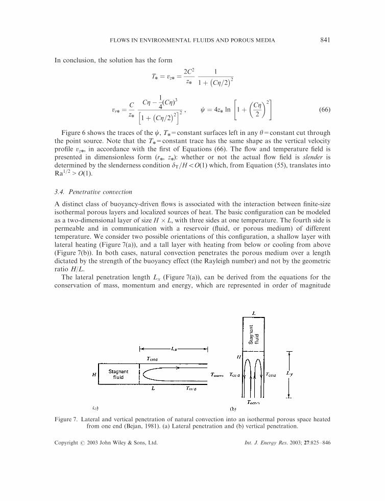
Figure 6 shows the traces of the c, Tn=constant surfaces left in any y=constant cut throughthe point source. Note that the Tn=constant trace has the same shape as the vertical velocityprofile vzn, in accordance with the first of Equations (66). The flow and temperature field ispresented in dimensionless form (rn, zn): whether or not the actual flow field is slender isdetermined by the slenderness condition dT=H5Oð1Þ which, from Equation (55), translates intoRa1=2 > Oð1Þ:

3.4. Penetrative convection

A distinct class of buoyancy-driven flows is associated with the interaction between finite-sizeisothermal porous layers and localized sources of heat. The basic configuration can be modeledas a two-dimensional layer of size H � L; with three sides at one temperature. The fourth side ispermeable and in communication with a reservoir (fluid, or porous medium) of differenttemperature. We consider two possible orientations of this configuration, a shallow layer withlateral heating (Figure 7(a)), and a tall layer with heating from below or cooling from above(Figure 7(b)). In both cases, natural convection penetrates the porous medium over a lengthdictated by the strength of the buoyancy effect (the Rayleigh number) and not by the geometricratio H/L.

The lateral penetration length Lx (Figure 7(a)), can be derived from the equations for theconservation of mass, momentum and energy, which are represented in order of magnitude

Figure 7. Lateral and vertical penetration of natural convection into an isothermal porous space heatedfrom one end (Bejan, 1981). (a) Lateral penetration and (b) vertical penetration.



terms byuLx

�vH

ð67Þ

uH

;vLx

�Kgbn

DTLx

ð68Þ

uDTLx

� aDTL2x

; aDTH2

ð69Þ

These three equations determine the unknown scales u, v, and Lx. Assuming that the flowpenetrates the layer such that Lx > H ; it is easy to show that

Lx � HRa1=2H ð70Þ

The convective heat transport between the isothermal porous layer and the heat reservoirpositioned laterally scales as

Q � rcPð ÞfHuDT � kDT Ra1=2H ð71Þ

where RaH ¼ KgbHT=ðanÞ: This heat transfer result demonstrates that the actual length of theporous layer (L) does not influence the heat transfer rate; Q and Lx are set by the Rayleighnumber RaH. The actual flow and temperature patterns associated with the lateral penetrationphenomenon can be determined analytically as a similarity solution (Bejan, 1981). Thepenetration length and heat transfer rate predicted by the similarity solution are Lx ¼ 0:158HRa

1=2H and Q=ðkT Þ ¼ 0:319 Ra

1=2H : The effect of anisotropy in the medium, and the effect of

temperature variation along the horizontal walls of the porous layer are also documented inBejan (1981).

In the vertical layer of Figure 7(b) the bottom wall is permeable and in communication with adifferent reservoir. Fluid motion sets in as soon as a DT is imposed between the bottom surfaceand vertical walls. Fluid motion is present because no matter how small the DT, the porousmedium experiences a finite-temperature gradient of order DT/L in the horizontal direction nearthe heated wall.

Let Ly be the distance of vertical penetration. The balances for mass, momentum and energyare

uL�

vLy

ð72Þ

uLy

;vL�

Kgbn

DTL

ð73Þ

uDTL

� aDTL2

; aDTL2y

ð74Þ

Assuming vertical penetration over a distance Ly greater than L, we conclude that

Ly � L RaL ð75Þ

where RaL is the Rayleigh number based on L, RaL ¼ KgbLT =ðanÞ: The net heat transfer ratethrough the bottom wall of the system scales as

Qy � ðrcP ÞfLvDT � kDTRaL ð76Þ


A. BEJAN842

In conclusion, both Ly and Qy are proportional to RaL, unlike the corresponding quantities inthe case of lateral penetration, which are proportional to Ra

1=2H : Once again, the imposed

temperature difference (DT) and the transversal dimension of the layer (L) determine thelongitudinal extent (Ly) of the penetrative flow. The physical height of the porous layer (H) doesnot influence the phenomenon as long as it is greater than Ly.

The phenomenon of partial vertical penetration was studied in the cylindrical geometry in anattempt to model geothermal flows (Bejan, 1980). The vertical penetration length and net heattransfer rate are Ly=r0 ¼ 0:0847 Rar0 and Qy=ðr0kDT Þ ¼ 0:255 Rar0 ; where Rar0 ¼ Kgbr0DT=ðanÞis the Rayleigh number based on the dimension normal to the penetrative flow (the cylindricalwell radius, r0).

4. OTHER CONFIGURATIONS

Environmental flows can be modelled in considerably more complex and diverse configurationsthan the free flows illustrated in this review. A distinct class are the flows that depend greatly onthe solid walls that confine them}in the extreme, the flows that occur in completely enclosedspaces. The study of flows in cavities filled with fluid and/or porous media saturated with fluidhas attracted a lot of interest during the last 2 decades. This body of work forms the subject ofseveral other review articles in this issue. Additional reviews may be found in the more recentreference books (e.g. Bejan, 1995; Jaluria, 1980; Kakac et al., 1985, 1987; Nield and Bejan, 1999).

The most complex configurations are in between. The study of flows that are partially ortemporarily free while confined by walls benefits from a good understanding of both extremes,free flows and enclosed flows. In closing, let us consider one such an example, namely the time-dependent Darcy flow due to the presence in a porous medium of two distinct regions (differenttemperatures and species concentrations) separated initially by a vertical interface (Figure 8,Zhang and Bejan, 1987). In time, the two regions share a counterflow that brings the entirespace to thermal and chemical equilibrium. The space is two dimensional with height H andhorizontal dimension L.

As an example of how two dissimilar adjacent regions come to equilibrium by convection,Figure 8 shows the evolution of the flow, temperature, and concentration fields of a relativelyhigh Rayleigh number flow driven by a buoyancy effect that is due entirely to density changescaused by temperature changes. This is also known as heat transfer driven flow. As the timeincreases, the warm fluid (initially on the left-hand side) migrates into the upper half of thesystem. The thermal barrier between the two thermal regions is smoothed gradually by thermaldiffusion. Figures 8(c) and 8(d) show that as the Lewis number decreases the sharpness of theconcentration dividing line disappears, as the phenomenon of mass diffusion becomes morepronounced.

In the case of heat transfer driven flows, the time scale associated with the end of convectivemass transfer in the horizontal direction is

#tt �js

� � LH

2

Ra�1 if Le Ra >js

LH

2

ð77Þ

#tt �js

� � LH

2

Le if Ra5js

LH

2

ð78Þ



The dimensionless time #tt is defined as #tt ¼ ðatÞ=ðsH2Þ: Values of #tt are listed on the side of eachframe of Figure 8. The Rayleigh number is Ra ¼ KgbHDT=ðanÞ; where DT is the initialtemperature difference between the two regions. The Lewis number definition is Le ¼ a=D;where D is the mass diffusivity of the chemical species. The time criteria (77) and (78) have beentested numerically along with the corresponding time scales for approach to thermal equilibrium.

Figure 8. The horizontal spreading and layering of thermal and chemical deposits in a porous mediumwhere natural convection is driven solely by temperature gradients (Ra ¼ 1000;H=L ¼ 1;j=s ¼ 1).

(a) Streamlines; (b) Isotherms, or isosolutal lines for Le ¼ 1 (Zhang and Bejan, 1987).

NOMENCLATURE

b =scale of jet (or plume) radius (m)b =stratification gradient (�dr/dy)


A. BEJAN844

bT =scale of thermal jet (or plume) radius (m)c =specific heat (J kg�1K�1)cP =specific heat at constant pressure (J kg�1K�1)C =volumetric concentration (kg m�3)C =constant, Equation (64)d =pore diameter (m)D =diameter, thickness (m)D =mass diffusivity (m2 s�1)fv =frequency of pulsating fire plume (s�1)F =similarity streamfunction, Equation (62)g =gravitational acceleration (m s�2)H =height (m)k =thermal conductivity (Wm�1K�1)K =jet strength (m4 s�2)K =permeability (m2)Lx,y =penetration distances (m)Le =Lewis number’mm =mass flow rate (kg s�1)’mm0 =mass flow rate per unit length (kg s�1m�1)P =pressure (Pa)q =heat transfer rate (W)q0 =heat transfer rate per unit length (Wm�1)q00 =heat flux (Wm�2)r =radial position (m)r0 =radius (m)Raq =Rayleigh number based on source strength, Equation (55)RaH,L =Rayleigh numbers based on temperature difference, Equations (71) and (75)St =Stanton numberT =temperature (K)u,v,w =velocity components (m s�1)U,V =velocity (m s�1)x,y =cartesian co-ordinates (m)

Greek symbols

a =thermal diffusivity (m2 s�1)#aa =constant, Equation (23)b =coefficient of volumetric thermal expansion (K�1)g =constant, Equation (9)dT =thermal thickness (m)DT =temperature difference (K)eH =thermal eddy diffusivity (m2 s�1)em =mass eddy diffusivity (m2 s�1)eM =momentum eddy diffusivity (m2 s�1)Z =similarity variablesy =angular position (rad)



REFERENCES

Bear J. 1972. Dynamics of Fluids in Porous Media. American Elsevier: New York.Bejan A. 1980. Natural convection in a vertical cylindrical well filled with porous medium. International Journal of Heat

and Mass Transfer 23:726–729.Bejan A. 1981. ‘Lateral intrusion of natural convection into a horizontal porous structure. Journal of Heat Transfer

103:237–241.Bejan A. 1991. Predicting the pool fire vortex shedding frequency. Journal of Heat Transfer 113:261–263.Bejan A. 1993. Heat Transfer. Wiley: New York.Bejan A. 1995. Convection Heat Transfer (2nd edn), Wiley: New York.Bejan A. 2000. Shape and Structure, from Engineering to Nature, Cambridge University Press: Cambridge, UK.Fischer HB, List EJ, Koh RCY, Imberger J, Brooks NH. 1979. Mixing in Inland and Coastal Waters, Chapter 9.

Academic Press: New York.Gebhart B, Jaluria Y, Mahajan RL, Sammakia B. 1988. Buoyancy-Induced Flows and Transport. Hemisphere: New

York.Greenkorn RA. 1983. Flow Phenomena in Porous Media. Marcel Dekker: New York.Jaluria Y. 1980. Natural Convection Heat and Mass Transfer. Pergamon: Oxford, 1980.Kakac S, Aung W, Viskanta R (eds). 1985. Natural Convection: Fundamentals and Applications. Hemisphere: New York.Kakac S, Shah RK, Aung W (eds). 1987. Handbook of Single-Phase Convective Heat Transfer. Wiley: New York.Nield DA, Bejan A. 1999. Convection in Porous Media (2nd edn). Springer: New York.Pagni PJ. 1989. Pool vortex shedding frequencies. In Some Unanswered Questions in Fluid Mechanics. Trefethen LM,

Panton RL (eds). ASME Paper No. 89-WA/FE-5.Prandtl L. 1969. Essentials of Fluid Dynamics. Blackie & Son: London, 122.Schlichting H. 1960. Boundary Layer Theory, (4th edn). McGraw-Hill, New York.Turner JS. 1973. Buoyancy Effects in Fluids, Cambridge University Press: Cambridge, UK.Zhang Z, Bejan A. 1987. The horizontal spreading of thermal and chemical deposits in a porous medium. International

Journal of Heat and Mass Transfer 37:129–138.

lB =buckling wavelength (m)m =viscosity (kg s�1m�1)n =kinematic viscosity (m2 s�1)r =density (kgm�3)s =capacity ratio, Equation (45)s =constant, Equation (5)f =porosityc =streamfunction

Superscript

� =time averaged

Subscripts

c =centrelinef =fluidr =radials =solidz =longitudinal0 =nozzle1 =ambientn =dimensionless, Equation (56)


A. BEJAN846

Documents

Flows in environmental fluids and porous media