FLOW THROUGH A DE LAVAL NOZZLE

Connor RobinsonComputational Fluid Dynamics, ME 702

December 20th, 2016

1

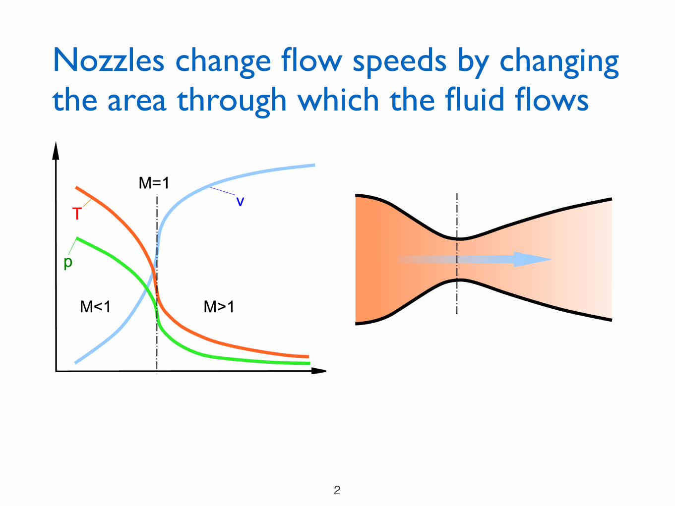
Nozzles change flow speeds by changing the area through which the fluid flows

2

We can gain physical insight about the flow using the governing equations

3

We can gain physical insight about the flow using the governing equations

4

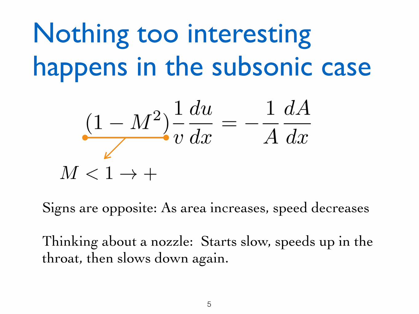
Nothing too interesting happens in the subsonic case

5

Signs are opposite: As area increases, speed decreases

Thinking about a nozzle: Starts slow, speeds up in the throat, then slows down again.

In the supersonic case, get smooth acceleration throughout the nozzle

6

Signs are the same: As area increases, speed increases

Thinking about a nozzle: Starts slow, speeds up in the throat, then continues to speed up!

This is known as a de Laval nozzle.

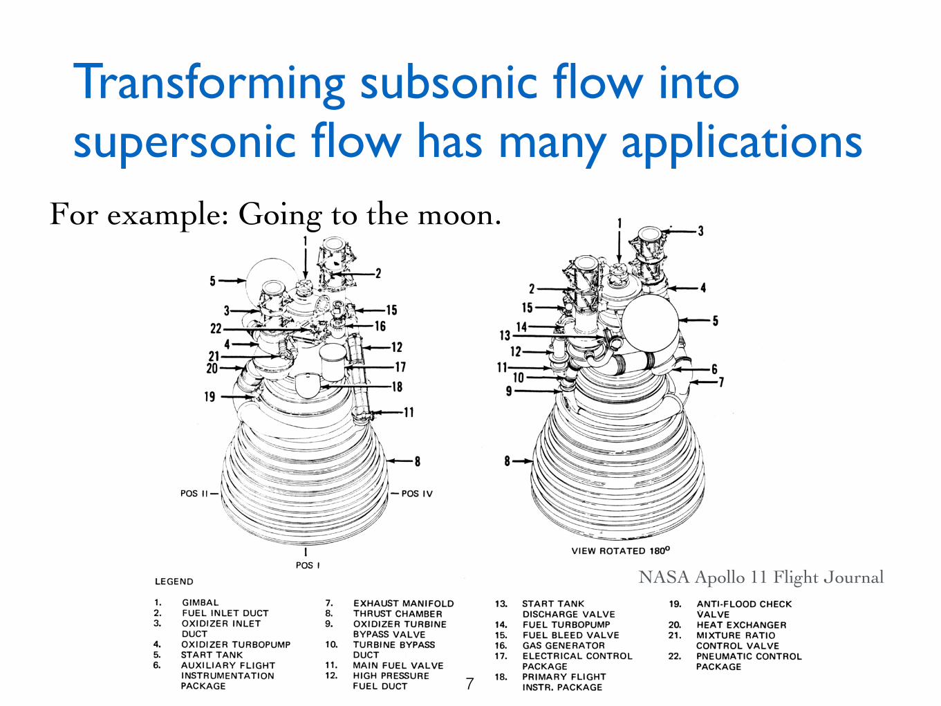
Transforming subsonic flow into supersonic flow has many applications

7

For example: Going to the moon.

NASA Apollo 11 Flight Journal

There are also astrophysical applications: Solar wind

8

Parker (1963)

Constructing the mesh for the nozzle

9

20

1

r[m]

z[m]

Cells: 400 x 200Transfinite scaling: 0.95

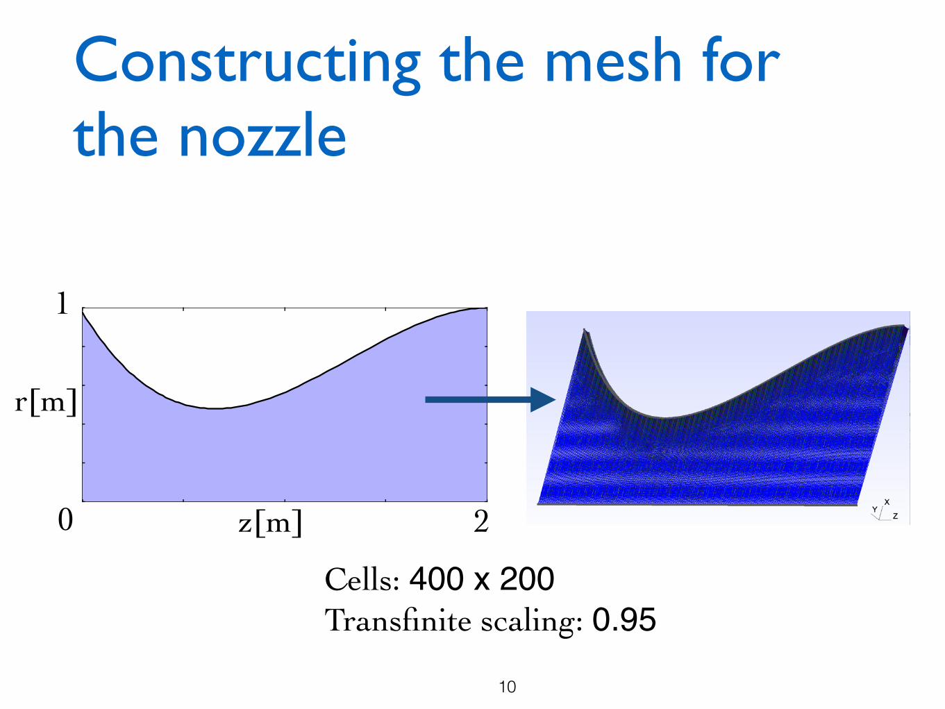
Constructing the mesh for the nozzle

10

20

1

r[m]

z[m]

Cells: 400 x 200Transfinite scaling: 0.95

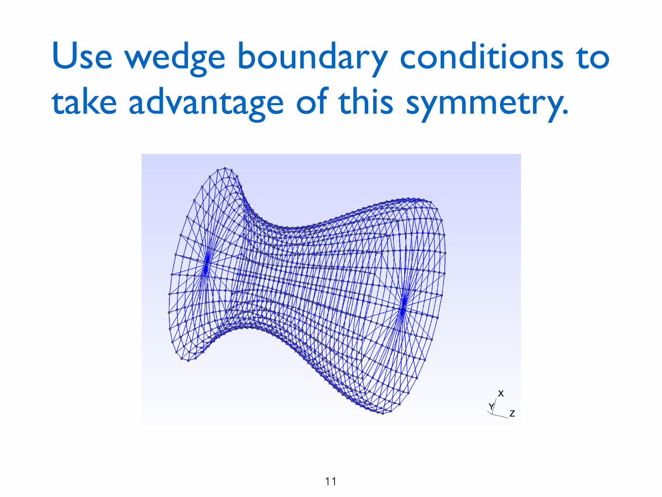
Use wedge boundary conditions to take advantage of this symmetry.

11

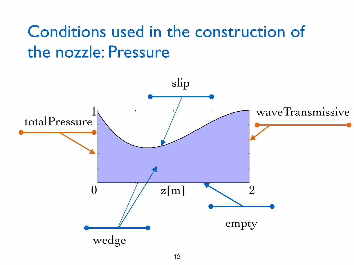
Conditions used in the construction of the nozzle: Pressure

12

20

1

z[m]

slip

waveTransmissivetotalPressure

emptywedge

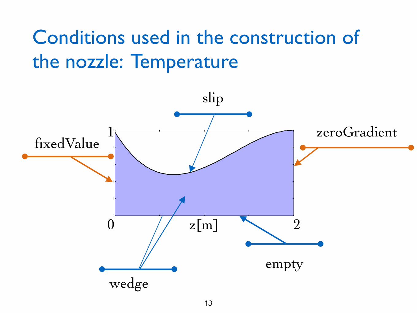
Conditions used in the construction of the nozzle: Temperature

13

20

1

z[m]

slip

zeroGradientfixedValue

emptywedge

Conditions used in the construction of the nozzle: Velocity

14

20

1

z[m]

slip

zeroGradientzeroGradient

emptywedge

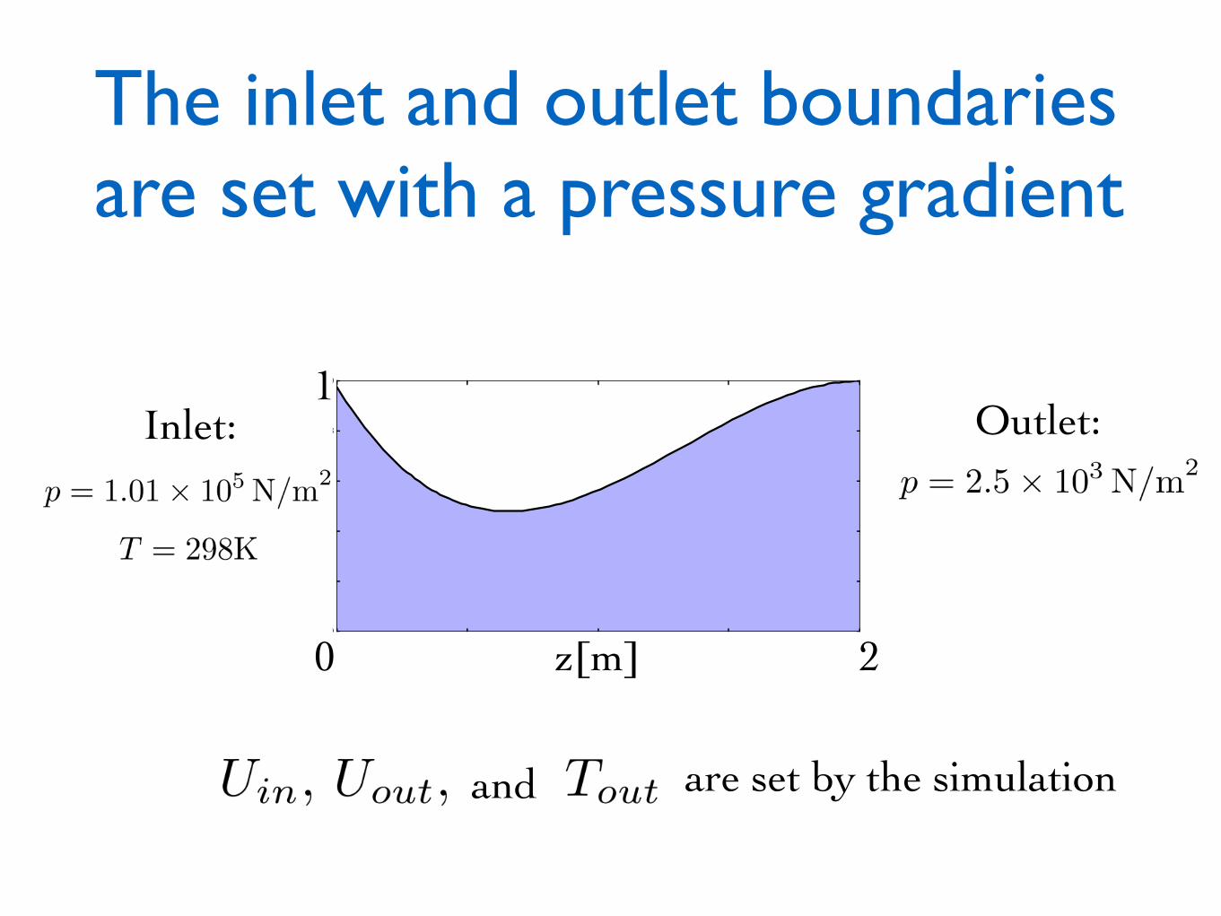
The inlet and outlet boundaries are set with a pressure gradient

15

20

1

z[m]

Inlet:

Outlet:

and are set by the simulation

Simulation uses the rhoCentralFoam solver

16

Density-based compressible flow solver based on central-upwind schemes

Uses Sutherland’s law to calculate the dynamic viscosity

Assumed the flow was laminar (no turbulence)

Initially get waves and shocks that dissipate over time

17

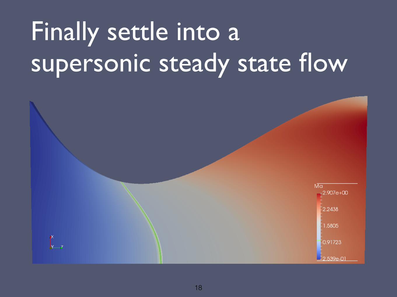
Finally settle into a supersonic steady state flow

18

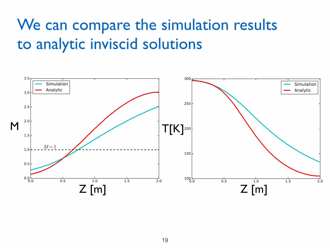
We can compare the simulation results to analytic inviscid solutions

19

M T[K]

Z [m]Z [m]

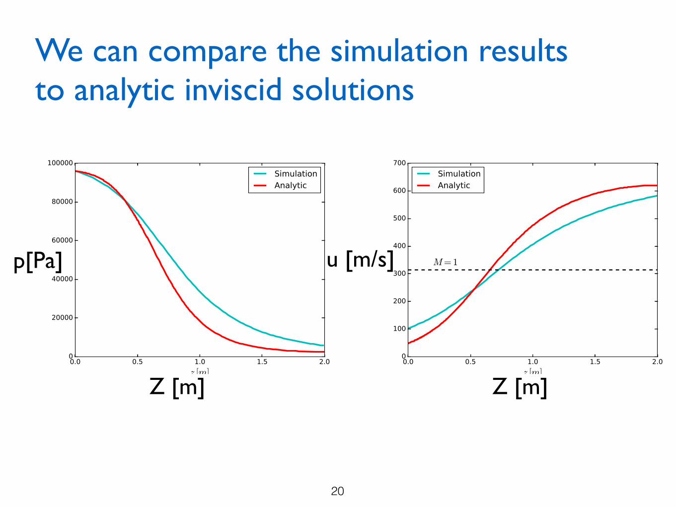
We can compare the simulation results to analytic inviscid solutions

20

p[Pa] u [m/s]

Z [m]Z [m]

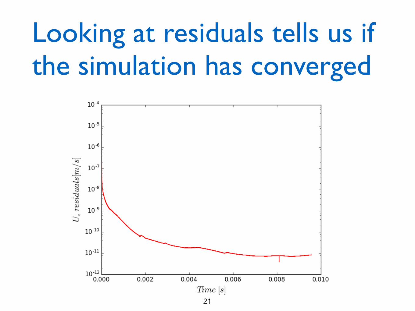
Looking at residuals tells us if the simulation has converged

21

Summary

• Nozzles can transition flow from subsonic to supersonic

• Built a flexible Python code that generates meshes that have cylindrical symmetry

• Using that mesh, set up a simulation of a supersonic de Laval nozzle that agrees with the analytic results quite well

22