Flow Regimes

PgDip/MSc Oil and Gas Engineering/Well Engineering Fundamenta1s Topic 9:Flow Regimes

© The Robert Gordon University 2001 1

Topic 9: Flow Regimes

Review

This section is intended for use by students to acquire a knowledge and understanding of flow regimes and fundamentals of pressure drop calculations.

Content

Flow in Pipes

Fluid flow is characterised by the following flow regimes:

• laminar: flows are stream line parallel to axis of conduit. No velocity component normal to direction of flow;

• turbulent: fluid components fluctuate in velocity in all directions;

• transitional flow represents the transition boundary from laminar to turbulent.

The criteria for determining the flow regime of a fluid is the Reynold’s number.

Reynold’s Number

Reynold’s number is calculated using Equation 1.

Equation 1.

s)-kg/m or (Ns/mVisosity

(m) Diameter,(m/s)velocity Average

)(kg/mDensity

Re

2

3

=µ

===ρ

µρ=

dv

dv

Reynold’s number is a dimensionless parameter. It is the main criteria used to define the flow regime of a fluid. The main flow regimes that engineers are interested in are Laminar and Turbulent flows.

If the cross sectional area is not circular, instead of d, the hydraulic diameter is used, calculated using Equation 2.

Equation 2.

fluid)by touched parts (all perimeter Wetted

area sectional CrossdiameterHydraulic

==

=

=

R

H

RH

PAd

PxA4d



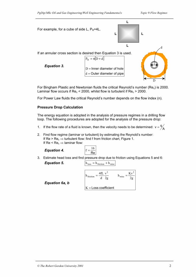
For example, for a cube of side L, PR=4L.

If an annular cross section is desired then Equation 3 is used.

Equation 3.

[ ]

pipe of diameter Outerhole of diameter Inner

==

+π=

dD

dDPR

For Bingham Plastic and Newtonian fluids the critical Reynold’s number (Rec) is 2000. Laminar flow occurs if Rec < 2000, whilst flow is turbulent if Rec > 2000.

For Power Law fluids the critical Reynold’s number depends on the flow index (n).

Pressure Drop Calculation

The energy equation is adopted in the analysis of pressure regimes in a drilling flow loop. The following procedures are adopted for the analysis of the pressure drop:

1. If the flow rate of a fluid is known, then the velocity needs to be determined: Aqv =

2. Find flow regime (laminar or turbulent) by estimating the Reynold’s number: If Re > Rec ⇒ turbulent flow: find f from friction chart, Figure 1. If Re < Rec ⇒ laminar flow:

Equation 4. Re16f =

3. Estimate head loss and find pressure drop due to friction using Equations 5 and 6: Equation 5. miscfrictionloss hhh +=

Equation 6a, b tcoefficien Loss

=

==

K

g2Kvh

g2v

dfL4h

2

misc

2

friction

L

L L

L

D

d



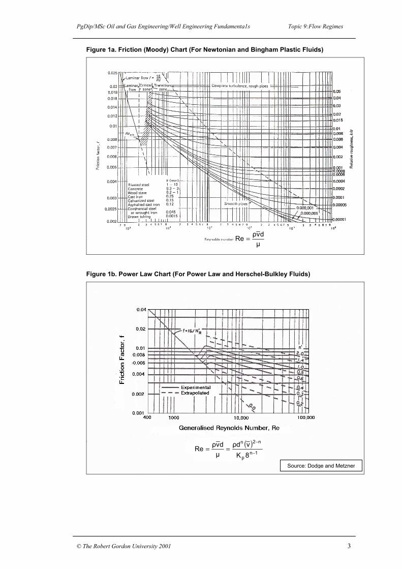
Figure 1a. Friction (Moody) Chart (For Newtonian and Bingham Plastic Fluids)

Figure 1b. Power Law Chart (For Power Law and Herschel-Bulkley Fluids)

µdvρRe =

( )1n

p

n2n

8Kvρd

µdvρRe

−

−==

Source: Dodge and Metzner



Flow Regimes

Flow regimes are relevant to the understanding of displacement efficiencies in a wellbore. Knowledge of flow regimes is important to the hole cleaning and cement displacement in the casing/hole annulus.

Laminar Flow

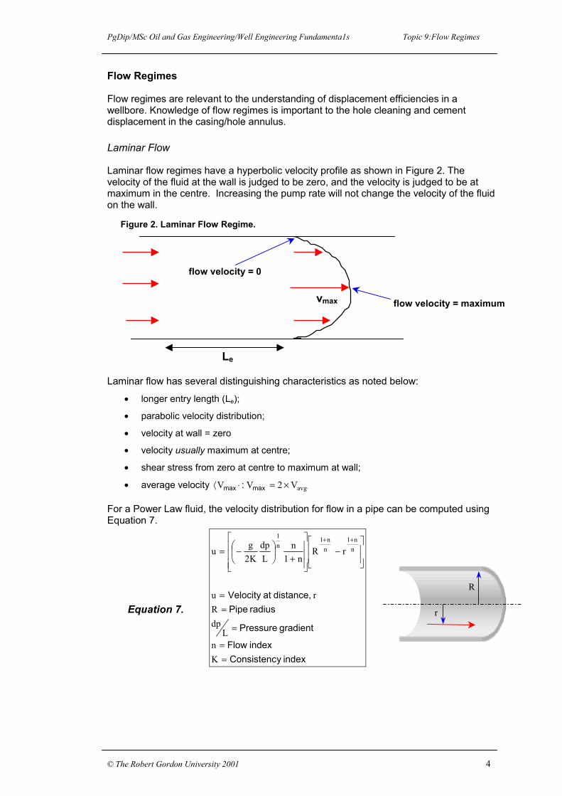
Laminar flow regimes have a hyperbolic velocity profile as shown in Figure 2. The velocity of the fluid at the wall is judged to be zero, and the velocity is judged to be at maximum in the centre. Increasing the pump rate will not change the velocity of the fluid on the wall.

Figure 2. Laminar Flow Regime.

Laminar flow has several distinguishing characteristics as noted below:

• longer entry length (Le);

• parabolic velocity distribution;

• velocity at wall = zero

• velocity usually maximum at centre;

• shear stress from zero at centre to maximum at wall;

• average velocity ⋅×=⋅⟨ avgV2VV maxmax :

For a Power Law fluid, the velocity distribution for flow in a pipe can be computed using Equation 7.

Equation 7.

indexy ConsistencindexFlow

gradient Pressure

radius Pipe distance, atVelocity

==

=

==

−

+

−=++

Kn

LdpR

ru

rRn1

nLdp

K2g

u nn1

nn1

n1

Le

vmax

flow velocity = 0

flow velocity = maximum

R

r



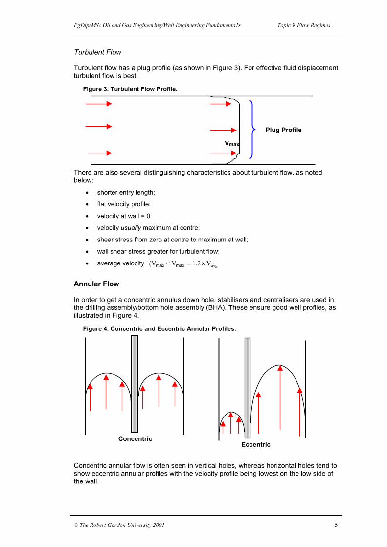
Turbulent Flow

Turbulent flow has a plug profile (as shown in Figure 3). For effective fluid displacement turbulent flow is best.

Figure 3. Turbulent Flow Profile.

There are also several distinguishing characteristics about turbulent flow, as noted below:

• shorter entry length;

• flat velocity profile;

• velocity at wall = 0

• velocity usually maximum at centre;

• shear stress from zero at centre to maximum at wall;

• wall shear stress greater for turbulent flow;

• average velocity ⋅×=⋅⟨ avgV21VV .: maxmax

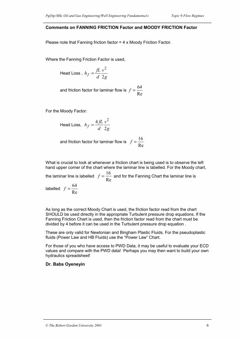
Annular Flow

In order to get a concentric annulus down hole, stabilisers and centralisers are used in the drilling assembly/bottom hole assembly (BHA). These ensure good well profiles, as illustrated in Figure 4.

Figure 4. Concentric and Eccentric Annular Profiles.

Concentric annular flow is often seen in vertical holes, whereas horizontal holes tend to show eccentric annular profiles with the velocity profile being lowest on the low side of the wall.

vmax

Plug Profile

Concentric Eccentric



Comments on FANNING FRICTION Factor and MOODY FRICTION Factor

Please note that Fanning friction factor = 4 x Moody Friction Factor.

Where the Fanning Friction Factor is used,

Head Loss , g

vdfLh f 2

2=

and friction factor for laminar flow is Re64=f

For the Moody Factor:

Head Loss, g

vdfLh f 2

4 2=

and friction factor for laminar flow is Re16=f

What is crucial to look at whenever a friction chart is being used is to observe the left hand upper corner of the chart where the laminar line is labelled. For the Moody chart,

the laminar line is labelled Re16=f and for the Fanning Chart the laminar line is

labelled Re64=f

As long as the correct Moody Chart is used, the friction factor read from the chart SHOULD be used directly in the appropriate Turbulent pressure drop equations. If the Fanning Friction Chart is used, then the friction factor read from the chart must be divided by 4 before it can be used in the Turbulent pressure drop equation .

These are only valid for Newtonian and Bingham Plastic Fluids. For the pseudoplastic fluids (Power Law and HB Fluids) use the “Power Law” Chart.

For those of you who have access to PWD Data, it may be useful to evaluate your ECD values and compare with the PWD data! Perhaps you may then want to build your own hydraulics spreadsheet!

Dr. Babs Oyeneyin

Documents

Flow Regimes